Nonlocal torque operators in ab initio theory of the Gilbert damping in random ferromagnetic alloys

Abstract

We present an ab initio theory of the Gilbert damping in substitutionally disordered ferromagnetic alloys. The theory rests on introduced nonlocal torques which replace traditional local torque operators in the well-known torque-correlation formula and which can be formulated within the atomic-sphere approximation. The formalism is sketched in a simple tight-binding model and worked out in detail in the relativistic tight-binding linear muffin-tin orbital (TB-LMTO) method and the coherent potential approximation (CPA). The resulting nonlocal torques are represented by nonrandom, non-site-diagonal and spin-independent matrices, which simplifies the configuration averaging. The CPA-vertex corrections play a crucial role for the internal consistency of the theory and for its exact equivalence to other first-principles approaches based on the random local torques. This equivalence is also illustrated by the calculated Gilbert damping parameters for binary NiFe and FeCo random alloys, for pure iron with a model atomic-level disorder, and for stoichiometric FePt alloys with a varying degree of L1₀ atomic long-range order.

I Introduction

The dynamics of magnetization of bulk ferromagnets, utrathin magnetic films and magnetic nanoparticles represents an important property of these systems, especially in the context of high speed magnetic devices for data storage. While a complete picture of magnetization dynamics including, e.g., excitation of magnons and their interaction with other degrees of freedom, is still a challenge for the modern theory of magnetism, remarkable progress has been achieved during the last years concerning the dynamics of the total magnetic moment, which can be probed experimentally by means of the ferromagnetic resonance Heinrich (1994) or by the time-resolved magneto-optical Kerr effect. Iihama et al. (2014) Time evolution of the macroscopic magnetization vector ${\bf M}$ can be described by the well-known Landau-Lifshitz-Gilbert (LLG) equation Pitaevskii and Lifshitz (1980); Gilbert (1955)

$$\frac{d{\bf M}}{dt}={\bf B}_{\rm eff}\times{\bf M}+\frac{\bf M}{M}\times\left(\underline{\bm{\alpha}}\cdot\frac{d{\bf M}}{dt}\right),$$ (1)

where ${\bf B}_{\rm eff}$ denotes an effective magnetic field (with the gyromagnetic ratio absorbed) acting on the magnetization, $M=|{\bf M}|$, and the quantity $\underline{\bm{\alpha}}=\{\alpha_{\mu\nu}\}$ denotes a symmetric $3\times 3$ tensor of the dimensionless Gilbert damping parameters ($\mu,\nu=x,y,z$). The first term in Eq. (1) defines a precession of the magnetization vector around the direction of the effective magnetic field and the second term describes a damping of the dynamics. The LLG equation in itinerant ferromagnets is appropriate for magnetization precessions very slow as compared to precessions of the single-electron spin due to the exchange splitting and to frequencies of interatomic electron hoppings.

A large number of theoretical approaches to the Gilbert damping has been worked out during the last two decades; here we mention only schemes within the one-electron theory of itinerant magnets, Kamberský (1976); Šimánek and Heinrich (2003); Sinova et al. (2004); Tserkovnyak et al. (2004); Steiauf and Fähnle (2005); Fähnle and Steiauf (2006); Gilmore et al. (2007); Kamberský (2007); Brataas et al. (2008); Gilmore et al. (2008); Garate and MacDonald (2009a, b); Starikov et al. (2010); Brataas et al. (2011); Ebert et al. (2011a); Sakuma (2012) where the most important effects of electron-electron interaction are captured by means of a local spin-dependent exchange-correlation (XC) potential. These techniques can be naturally combined with existing first-principles techniques based on the density-functional theory, which leads to parameter-free calculations of the Gilbert damping tensor of pure ferromagnetic metals, their ordered and disordered alloys, diluted magnetic semiconductors, etc. One part of these approaches is based on a static limit of the frequency-dependent spin-spin correlation function of a ferromagnet. Kamberský (1976); Šimánek and Heinrich (2003); Sinova et al. (2004); Tserkovnyak et al. (2004); Garate and MacDonald (2009a, b) Other routes to the Gilbert damping employ relaxations of occupation numbers of individual Bloch electron states during quasi-static nonequilibrium processes or transition rates between different states induced by the spin-orbit (SO) interaction. Steiauf and Fähnle (2005); Fähnle and Steiauf (2006); Gilmore et al. (2007); Kamberský (2007); Gilmore et al. (2008); Sakuma (2012) The dissipation of magnetic energy accompanying the slow magnetization dynamics, evaluated within a scattering theory or the Kubo linear response formalism, leads also to explicit expressions for the Gilbert damping tensor. Brataas et al. (2008); Starikov et al. (2010); Brataas et al. (2011); Ebert et al. (2011a) Most of these formulations yield relations equivalent to the so-called torque-correlation formula

$$\alpha_{\mu\nu}=-\alpha_{0}{\rm Tr}\{T_{\mu}(G_{+}-G_{-})T_{\nu}(G_{+}-G_{-})\},$$ (2)

in which the torque operators $T_{\mu}$ are either due to the XC or SO terms of the one-electron Hamiltonian. In Eq. (2), which has a form of the Kubo-Greenwood formula and is valid for zero temperature of electrons, the quantity $\alpha_{0}$ is related to the system magnetization (and to fundamental constants and units used, see Section II.2), the trace is taken over the whole Hilbert space of valence electrons, and the symbols $G_{\pm}=G(E_{\rm F}\pm{\rm i}0)$ denote the one-particle retarded and advanced propagators (Green’s functions) at the Fermi energy $E_{\rm F}$.

Implementation of the above-mentioned theories in first-principles computational schemes proved opposite trends of the intraband and interband contributions to the Gilbert damping parameter as functions of a phenomenological quasiparticle lifetime broadening. Sinova et al. (2004); Gilmore et al. (2007); Kamberský (2007) These qualitative studies have recently been put on a more solid basis by considering a particular mechanism of the lifetime broadening, namely, a frozen temperature-induced structural disorder, which represents a realistic model for a treatment of temperature dependence of the Gilbert damping. Liu et al. (2011); Mankovsky et al. (2013) This approach explained quantitatively the low-temperature conductivity-like and high-temperature resistivity-like trends of the damping parameters of iron, cobalt and nickel. Further improvements of the model, including static temperature-induced random orientations of local magnetic moments, have appeared recently. Ebert et al. (2015)

The ab initio studies have also been successful in reproduction and interpretation of values and concentration trends of the Gilbert damping in random ferromagnetic alloys, such as the NiFe alloy with the face-centered cubic (fcc) structure (Permalloy) Starikov et al. (2010); Mankovsky et al. (2013) and Fe-based alloys with the body-centered cubic (bcc) structure (FeCo, FeV, FeSi). Ebert et al. (2011a); Barsukov et al. (2011); Mankovsky et al. (2013) Other studies addressed also the effects of doping the Permalloy and bcc iron by $5d$ transition-metal elements Ebert et al. (2011a); Sakuma (2012); Mankovsky et al. (2013) and of the degree of atomic long-range order in equiconcentration FeNi and FePt alloys with the L1₀-type structures. Sakuma (2012) Recently, an application to halfmetallic Co-based Heusler alloys has appeared as well. Sakuma (2015a) The obtained results revealed correlations of the damping parameter with the density of states at the Fermi energy and with the size of magnetic moments. Barsukov et al. (2011); Mankovsky et al. (2013)

In a one-particle mean-field-like description of a ferromagnet, the total spin is not conserved due to the XC field and the SO interaction. The currently employed forms of the torque operators $T_{\mu}$ in the torque-correlation formula (2) reflect these two sources; both the XC- and the SO-induced torques are local and their equivalence for the theory of Gilbert damping has been discussed by several authors. Garate and MacDonald (2009a, b); Sakuma (2015b) In the case of random alloys, this equivalence rests on a proper inclusion of vertex corrections in the configuration averaging of the damping parameters $\alpha_{\mu\nu}$ as two-particle quantities.

The purpose of the present paper is to introduce another torque operator that can be used in the torque-correlation formula (2) and to discuss its properties. This operator is due to intersite electron hopping and it is consequently nonlocal; in contrast to the local XC- and SO-induced torques which are random in random crystalline alloys, the nonlocal torque is nonrandom, i.e., independent on the particular configuration of a random alloy, which simplifies the configuration averaging of Eq. (2). We show that a similar nonlocal effective torque appears in the fully relativistic linear muffin-tin orbital (LMTO) method in the atomic-sphere approximation (ASA) used recently for calculations of the conductivity tensor in spin-polarized random alloys. Turek et al. (2012a, 2014) Here we discuss theoretical aspects of the averaging in the coherent-potential approximation (CPA) Velický (1969); Carva et al. (2006) and illustrate the developed ab initio scheme by applications to selected binary alloys. We also compare the obtained results with those of the LMTO-supercell technique Starikov et al. (2010) and with other CPA-based techniques, the fully relativistic Korringa-Kohn-Rostoker (KKR) method Ebert et al. (2011a); Mankovsky et al. (2013) and the LMTO method with a simplified treatment of the SO interaction. Sakuma (2012)

The paper is organized as follows. The theoretical formalism is contained in Section II, with a general discussion of various torque operators and results of a simple tight-binding model presented in Section II.1. The following Section II.2 describes the derivation of the LMTO torque-correlation formula with nonlocal torques; technical details are left to Appendix A concerning linear-response calculations with varying basis sets and to Appendix B regarding the LMTO method for systems with a tilted magnetization direction. Selected formal properties of the developed theory are discussed in Section II.3. Applications of the developed formalism can be found in Section III. Details of numerical implementation are listed in Section III.1 followed by illustrating examples for systems of three different kinds: binary solid solutions of $3d$ transition metals in Section III.2, pure iron with a simple model of random potential fluctuations in Section III.3, and stoichiometric FePt alloys with a partial long-range order in Section III.4. The main conclusions are summarized in Section IV.

II Theoretical formalism

II.1 Torque-correlation formula with alternative torque operators

The torque operators $T_{\mu}$ entering the torque-correlation formula (2) are closely related to components of the time derivative of electron spin. For spin-polarized systems described by means of an effective Schrödinger-Pauli one-electron Hamiltonian $H$, acting on two-component wave functions, the complete time derivative of the spin operator is given by the commutation relation $t_{\mu}=-{\rm i}[\sigma_{\mu}/2,H]$, where $\hbar=1$ is assumed and $\sigma_{\mu}$ ($\mu=x,y,z$) denote the Pauli spin matrices. Let us write the Hamiltonian as $H=H^{\rm p}+H^{\rm xc}$, where $H^{\rm p}$ includes all spin-independent terms and the SO interaction (Hamiltonian of a paramagnetic system) while $H^{\rm xc}={\bf B}^{\rm xc}({\bf r})\cdot\bm{\sigma}$ denotes the XC term due to an effective magnetic field ${\bf B}^{\rm xc}({\bf r})$. The complete time derivative (spin torque) can then be written as $t_{\mu}=t^{\rm so}_{\mu}+t^{\rm xc}_{\mu}$, where

$$t^{\rm so}_{\mu}=-{\rm i}[\sigma_{\mu}/2,H^{\rm p}],\qquad t^{\rm xc}_{\mu}=-{\rm i}[\sigma_{\mu}/2,H^{\rm xc}].$$ (3)

As discussed, e.g., in Ref. Garate and MacDonald, 2009a, the use of the complete torque $t_{\mu}$ in the torque-correlation formula (2) leads identically to zero; the correct Gilbert damping coefficients $\alpha_{\mu\nu}$ follow from Eq. (2) by using either the SO-induced torque $t^{\rm so}_{\mu}$, or the XC-induced torque $t^{\rm xc}_{\mu}$. Note that only transverse components (with respect to the easy axis of the ferromagnet) of the vectors ${\bf t}^{\rm so}$ and ${\bf t}^{\rm xc}$ are needed for the relevant part of the Gilbert damping tensor (2).

The equivalence of both torque operators (3) for the Gilbert damping can be extended. Let us consider a simple system described by a model tight-binding Hamiltonian $H$, written now as $H=H^{\rm loc}+H^{\rm nl}$, where the first term $H^{\rm loc}$ is a lattice sum of local atomic-like terms and the nonlocal second term $H^{\rm nl}$ includes all intersite hopping matrix elements. Let us assume that all effects of the SO interaction and XC fields are contained in the local term $H^{\rm loc}$, so that the hopping elements are spin-independent and $[\sigma_{\mu},H^{\rm nl}]=0$. (Note that this assumption, often used in model studies, is satisfied only approximatively in real ferromagnets with different widths of the majority and minority spin bands.) Let us write explicitly $H^{\rm loc}=\sum_{\bf R}(H^{\rm p}_{\bf R}+H^{\rm xc}_{\bf R})$, where ${\bf R}$ labels the lattice sites and where $H^{\rm p}_{\bf R}$ comprises the spin-independent part and the SO interaction of the ${\bf R}$th atomic potential while $H^{\rm xc}_{\bf R}$ is due to the local XC field of the ${\bf R}$th atom. The operators $H^{\rm p}_{\bf R}$ and $H^{\rm xc}_{\bf R}$ act only in the subspace of the ${\bf R}$th site; the subspaces of different sites are orthogonal to each other. The total spin operator can be written as $\sigma_{\mu}/2=(1/2)\sum_{\bf R}\sigma_{{\bf R}\mu}$, where the local operator $\sigma_{{\bf R}\mu}$ is the projection of $\sigma_{\mu}$ on the ${\bf R}$th subspace. Let us assume that each term $H^{\rm p}_{\bf R}$ is spherically symmetric and that $H^{\rm xc}_{\bf R}={\bf B}^{\rm xc}_{\bf R}\cdot\bm{\sigma}_{\bf R}$, where the effective field ${\bf B}^{\rm xc}_{\bf R}$ of the ${\bf R}$th atom has a constant size and direction. Let us introduce local orbital-momentum operators $L_{{\bf R}\mu}$ and their counterparts including the spin, $J_{{\bf R}\mu}=L_{{\bf R}\mu}+(\sigma_{{\bf R}\mu}/2)$, which are generators of local infinitesimal rotations with respect to the ${\bf R}$th lattice site, and let us define the corresponding lattice sums $L_{\mu}=\sum_{\bf R}L_{{\bf R}\mu}$ and $J_{\mu}=\sum_{\bf R}J_{{\bf R}\mu}=L_{\mu}+(\sigma_{\mu}/2)$. Then the local terms $H^{\rm p}_{\bf R}$ and $H^{\rm xc}_{\bf R}$ satisfy, respectively, commutation rules $[J_{{\bf R}\mu},H^{\rm p}_{\bf R}]=0$ and $[L_{{\bf R}\mu},H^{\rm xc}_{\bf R}]=0$. By using the above assumptions and definitions, the XC-induced spin torque (3) due to the XC term $H^{\rm xc}=\sum_{\bf R}H^{\rm xc}_{\bf R}$ can be reformulated as

$$t^{\rm xc}_{\mu} = -{\rm i}\sum_{\bf R}[\sigma_{{\bf R}\mu}/2,H^{\rm xc}_{\bf R}]=-{\rm i}\sum_{\bf R}[J_{{\bf R}\mu},H^{\rm xc}_{\bf R}]$$

$$= -{\rm i}\sum_{\bf R}[J_{{\bf R}\mu},H^{\rm p}_{\bf R}+H^{\rm xc}_{\bf R}]=-{\rm i}[J_{\mu},H^{\rm loc}]\equiv t^{\rm loc}_{\mu}.$$

The last commutator defines a local torque operator $t^{\rm loc}_{\mu}$ due to the local part of the Hamiltonian $H^{\rm loc}$ and the operator $J_{\mu}$, in contrast to the spin operator $\sigma_{\mu}/2$ in Eq. (3). Let us define the complementary nonlocal torque $t^{\rm nl}_{\mu}$ due to the nonlocal part of the Hamiltonian $H^{\rm nl}$, namely,

$$t^{\rm nl}_{\mu}=-{\rm i}[J_{\mu},H^{\rm nl}]=-{\rm i}[L_{\mu},H^{\rm nl}],$$ (5)

and let us employ the fact that the complete time derivative of the operator $J_{\mu}$, i.e., the torque $\tilde{t}_{\mu}=-{\rm i}[J_{\mu},H]=t^{\rm loc}_{\mu}+t^{\rm nl}_{\mu}$, leads identically to zero when used in Eq. (2). This fact implies that the Gilbert damping parameters can be also obtained from the torque-correlation formula with the nonlocal torques $t^{\rm nl}_{\mu}$. These torques are equivalent to the original spin-dependent local XC- or SO-induced torques; however, the derived nonlocal torques are spin-independent, so that commutation rules $[t^{\rm nl}_{\mu},\sigma_{\nu}]=0$ are satisfied.

In order to see the effect of different forms of the torque operators, Eqs. (3) and (5), we have studied a tight-binding model of $p$-orbitals on a simple cubic lattice with the ground-state magnetization along $z$ axis. The local (atomic-like) terms of the Hamiltonian are specified by the XC term $b\sigma_{{\bf R}z}$ and the SO term $\xi{\bf L}_{\bf R}\cdot\bm{\sigma}_{\bf R}$, which are added to a random spin-independent $p$-level at energy $\epsilon_{0}+D_{\bf R}$, where $\epsilon_{0}$ denotes the nonrandom center of the $p$-band while the random parts $D_{\bf R}$ satisfy configuration averages $\langle D_{\bf R}\rangle=0$ and $\langle D_{{\bf R}^{\prime}}D_{\bf R}\rangle=\gamma\delta_{{\bf R}^{\prime}{\bf R}}$ with the disorder strength $\gamma$. The spin-independent nonlocal (hopping) part of the Hamiltonian has been confined to nonrandom nearest-neighbor hoppings parametrized by two quantities, $W_{1}$ ($pp\sigma$ hopping) and $W^{\prime}_{1}$ ($pp\pi$ hopping), see, e.g., page 36 of Ref. Gonis, 1992. The particular values have been set to $b=0.3$, $\xi=0.2$, $E_{\rm F}-\epsilon_{0}=0.1$, $\gamma=0.05$, $W_{1}=0.3$ and $W^{\prime}_{1}=-0.1$ (the hoppings were chosen such that the band edges for $\epsilon_{0}=b=\xi=\gamma=0$ are $\pm 1$). The configuration average of the propagators $\langle G_{\pm}\rangle=\bar{G}_{\pm}$ and of the torque correlation (2) was performed in the self-consistent Born approximation (SCBA) including the vertex corrections. Since all three torques, Eqs. (3) and (5), are nonrandom operators in our model, the only relevant component of the Gilbert damping tensor, namely $\alpha_{xx}=\alpha_{yy}=\alpha$, could be unambiguously decomposed in the coherent part $\alpha^{\rm coh}$ and the incoherent part $\alpha^{\rm vc}$ due to the vertex corrections.

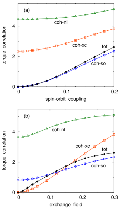
Figure 1: (Color online) The torque correlation $\alpha/\alpha_{0}$, Eq. (2), in a tight-binding $p$-orbital model treated in the SCBA as a function of the spin-orbit coupling $\xi$ (a) and of the exchange field $b$ (b). The full diamonds display the total torque correlation (tot) and the open symbols denote the coherent contributions $\alpha^{\rm coh}/\alpha_{0}$ calculated with the SO-induced torque (coh-so), the XC-induced torque (coh-xc), Eq. (3), and the nonlocal torque (coh-nl), Eq. (5).

The results are summarized in Fig. 1 which displays the torque correlation $\alpha/\alpha_{0}$ as a function of the SO coupling $\xi$ (Fig. 1a) and the XC field $b$ (Fig. 1b). The total value $\alpha=\alpha^{\rm coh}+\alpha^{\rm vc}$ is identical for all three forms of the torque operator, in contrast to the coherent parts $\alpha^{\rm coh}$ which exhibit markedly different values and trends as compared to each other and to the total $\alpha$. This result is in line with conclusions drawn by the authors of Ref. Garate and MacDonald, 2009a, b; Sakuma, 2015b proving the importance of the vertex corrections for obtaining the same Gilbert damping parameters from the SO- and XC-induced torques. The only exception seems to be the case of the SO splitting much weaker than the exchange splitting, where the vertex corrections for the SO-induced torque can be safely neglected, see Fig. 1a. This situation, encountered in $3d$ transition metals and their alloys, has been treated with the SO-induced torque on an ab initio level with neglected vertex corrections in Ref. Gilmore et al., 2007; Kamberský, 2007. On the other hand, the use of the XC-induced torque calls for a proper evaluation of the vertex corrections; their neglect leads to quantitatively and physically incorrect results as documented by recent first-principles studies. Ebert et al. (2011a); Mankovsky et al. (2013) The vertex corrections are indispensable also for the nonlocal torque, in particular for correct vanishing of the total torque correlation both in the nonrelativistic limit ($\xi\to 0$, Fig. 1a) and in the nonmagnetic limit ($b\to 0$, Fig. 1b).

Finally, let us discuss briefly the general equivalence of the SO- and XC-induced spin torques, Eq. (3), in the fully relativistic four-component Dirac formalism. Zabloudil et al. (2005); Ebert et al. (2011b) The Kohn-Sham-Dirac Hamiltonian can be written as $H=H^{\rm p}+H^{\rm xc}$, where $H^{\rm p}=c\bm{\alpha}\cdot{\bf p}+mc^{2}\beta+V({\bf r})$ and $H^{\rm xc}={\bf B}^{\rm xc}({\bf r})\cdot\beta\bm{\Sigma}$, where $c$ is the speed of light, $m$ denotes the electron mass, ${\bf p}=\{p_{\mu}\}$ refers to the momentum operator, $V({\bf r})$ is the spin-independent part of the effective potential and the $\bm{\alpha}=\{\alpha_{\mu}\}$, $\beta$ and $\bm{\Sigma}=\{\Sigma_{\mu}\}$ are the well-known $4\times 4$ matrices of the Dirac theory. Rose (1961); Strange (1998) Then the XC-induced torque is ${\bf t}^{\rm xc}={\bf B}^{\rm xc}({\bf r})\times\beta\bm{\Sigma}$, which is currently used in the KKR theory of the Gilbert damping. Ebert et al. (2011a); Mankovsky et al. (2013) The SO-induced torque is ${\bf t}^{\rm so}={\bf p}\times c\bm{\alpha}$, i.e., it is given directly by the relativistic momentum (${\bf p}$) and velocity ($c\bm{\alpha}$) operators. One can see that the torque ${\bf t}^{\rm so}$ is local but independent of the particular system studied. A comparison of both alternatives, concerning the total damping parameters as well as their coherent and incoherent parts, would be desirable; however, this task is beyond the scope of the present study.

II.2 Effective torques in the LMTO method

In our ab initio approach to the Gilbert damping, we employ the torque-correlation formula (2) with torques derived from the XC field. Garate and MacDonald (2009a); Ebert et al. (2011a); Mankovsky et al. (2013) The torque operators are constructed by considering infinitesimal deviations of the direction of the XC field of the ferromagnet from its equilibrium orientation, taken as a reference state. These deviations result from rotations by small angles around axes perpendicular to the equilibrium direction of the XC field; components of the torque operator are then given as derivatives of the one-particle Hamiltonian with respect to the rotation angles. Carva and Turek (2009)

For practical evaluation of Eq. (2) in an ab initio technique (such as the LMTO method), one has to consider a matrix representation of all operators in a suitable orthonormal basis. The most efficient techniques of the electronic structure theory require typically basis vectors tailored to the system studied; in the present context, this leads naturally to basis sets depending on the angular variables needed to define the torque operators. Evaluation of the torque correlation using angle-dependent bases is discussed in Appendix A, where we prove that Eq. (2) can be calculated solely from the matrix elements of the Hamiltonian and their angular derivatives, see Eq. (20), whereas the angular dependence of the basis vectors does not contribute directly to the final result.

The relativistic LMTO-ASA Hamiltonian matrix for the reference system in the orthogonal LMTO representation is given by Solovyev et al. (1991); Shick et al. (1996); Turek et al. (1997)

$$H=C+(\sqrt{\Delta})^{+}S(1-\gamma S)^{-1}\sqrt{\Delta},$$ (6)

where the $C$, $\sqrt{\Delta}$ and $\gamma$ denote site-diagonal matrices of the standard LMTO potential parameters and $S$ is the matrix of canonical structure constants. The change of the Hamiltonian matrix $H$ due to a uniform rotation of the XC field is treated in Appendix B; it is summarized for finite rotations in Eq. (27) and for angular derivatives of $H$ in Eqs. (28) and (29). The resolvent $G(z)=(z-H)^{-1}$ of the LMTO Hamiltonian (6) for complex energies $z$ can be expressed using the auxiliary resolvent $g(z)=[P(z)-S]^{-1}$, which represents an LMTO-counterpart of the scattering-path operator matrix of the KKR method. Zabloudil et al. (2005); Ebert et al. (2011b) The symbol $P(z)$ denotes the site-diagonal matrix of potential functions; their analytic dependence on $z$ and on the potential parameters can be found elsewhere. Solovyev et al. (1991); Turek et al. (2012a) The relation between both resolvents leads to the formula Turek et al. (2014)

$$G_{+}-G_{-}=F(g_{+}-g_{-})F^{+},$$ (7)

where the same abbreviation $F=(\sqrt{\Delta})^{-1}(1-\gamma S)$ as in Eq. (28) was used and $g_{\pm}=g(E_{\rm F}\pm{\rm i}0)$ .

The torque-correlation formula (2) in the LMTO-ASA method follows directly from relations (20), (28), (29) and (7). The components of the Gilbert damping tensor $\{\alpha_{\mu\nu}\}$ in the LLG equation (1) can be obtained from a basic tensor $\{{\tilde{\alpha}}_{\mu\nu}\}$ given by

$${\tilde{\alpha}}_{\mu\nu}=-\alpha_{0}\,{\rm Tr}\{\tau_{\mu}(g_{+}-g_{-})\tau_{\nu}(g_{+}-g_{-})\},$$ (8)

where the quantities

$$\tau_{\mu}=-{\rm i}[{\cal J}^{\mu},S]=-{\rm i}[{\cal L}^{\mu},S]$$ (9)

define components of an effective torque in the LMTO-ASA method. The site-diagonal matrices ${\cal J}^{\mu}$ and ${\cal L}^{\mu}$ ($\mu=x,y,z$) are Cartesian components of the total and orbital angular momentum operator, respectively, see text around Eqs. (28) and (29). The trace in (8) extends over all orbitals of the crystalline solid and the prefactor can be written as $\alpha_{0}=(2\pi M_{\rm spin})^{-1}$, where $M_{\rm spin}$ denotes the spin magnetic moment of the whole crystal in units of the Bohr magneton $\mu_{\rm B}$. Garate and MacDonald (2009a); Ebert et al. (2011a); Mankovsky et al. (2013)

Let us discuss properties of the effective torque (9). Its form is obviously identical to the nonlocal torque (5). The matrix $\tau_{\mu}$ is non-site-diagonal, but—for a random substitutional alloy on a nonrandom lattice—it is nonrandom (independent on the alloy configuration). Moreover, it is given by a commutator of the site-diagonal nonrandom matrix ${\cal J}^{\mu}$ (or ${\cal L}^{\mu}$) and the LMTO structure-constant matrix $S$. These properties point to a close analogy between the effective torque and the effective velocities in the LMTO conductivity tensor based on a concept of intersite electron hopping. Turek et al. (2002, 2012a, 2014) Let us mention that existing ab initio approaches employ random torques, either the XC-induced torque in the KKR method Ebert et al. (2011a); Mankovsky et al. (2013) or the SO-induced torque in the LMTO method. Sakuma (2012) Another interesting property of the effective torque $\tau_{\mu}$ (9) is its spin-independence which follows from the spin-independence of the matrices ${\cal L}^{\mu}$ and $S$.

The explicit relation between the symmetric tensors $\{\alpha_{\mu\nu}\}$ and $\{{\tilde{\alpha}}_{\mu\nu}\}$ can be easily formulated for the ground-state magnetization along $z$ axis; then it is given simply by $\alpha_{xx}={\tilde{\alpha}}_{yy}$, $\alpha_{yy}={\tilde{\alpha}}_{xx}$, and $\alpha_{xy}=-{\tilde{\alpha}}_{xy}$. These relations reflect the fact that an infinitesimal deviation towards $x$ axis results from an infinitesimal rotation of the magnetization vector around $y$ axis and vice versa. Note that the other components of the Gilbert damping tensor ($\alpha_{\mu z}$ for $\mu=x,y,z$) are not relevant for the dynamics of small deviations of magnetization direction described by the LLG equation (1). For the ground-state magnetization pointing along a general unit vector ${\bf m}=(m_{x},m_{y},m_{z})$, one has to employ the Levi-Civita symbol $\epsilon_{\mu\nu\lambda}$ in order to get the Gilbert damping tensor $\underline{\bm{\alpha}}$ as

$$\alpha_{\mu\nu}=\sum_{\mu^{\prime}\nu^{\prime}}\eta_{\mu\mu^{\prime}}\eta_{\nu\nu^{\prime}}{\tilde{\alpha}}_{\mu^{\prime}\nu^{\prime}},$$ (10)

where $\eta_{\mu\nu}=\sum_{\lambda}\epsilon_{\mu\nu\lambda}m_{\lambda}$. The resulting tensor $(\ref{eq_altal})$ satisfies the condition $\underline{\bm{\alpha}}\cdot{\bf m}=0$ appropriate for the dynamics of small transverse deviations of magnetization.

The application to random alloys requires configuration averaging of ${\tilde{\alpha}}_{\mu\nu}$ (8). Since the effective torques $\tau_{\mu}$ are nonrandom, one can write a unique decomposition of the average into the coherent and incoherent parts, ${\tilde{\alpha}}_{\mu\nu}={\tilde{\alpha}}^{\rm coh}_{\mu\nu}+{\tilde{\alpha}}^{\rm vc}_{\mu\nu}$, where the coherent part is expressed by means of the averaged auxiliary resolvents ${\bar{g}}_{\pm}=\langle g_{\pm}\rangle$ as

$${\tilde{\alpha}}^{\rm coh}_{\mu\nu}=-\alpha_{0}{\rm Tr}\{\tau_{\mu}({\bar{g}}_{+}-{\bar{g}}_{-})\tau_{\nu}({\bar{g}}_{+}-{\bar{g}}_{-})\}$$ (11)

and the incoherent part (vertex corrections) is given as a sum of four terms, namely,

$${\tilde{\alpha}}^{\rm vc}_{\mu\nu}=-\alpha_{0}\sum_{p=\pm}\sum_{q=\pm}{\rm sgn}(pq){\rm Tr}\langle\tau_{\mu}g_{p}\tau_{\nu}g_{q}\rangle_{\rm vc}.$$ (12)

In this work, the configuration averaging has been done in the CPA. Details concerning the averaged resolvents can be found, e.g., in Ref. Turek et al., 1997 and the construction of the vertex corrections for transport properties was described in Appendix to Ref. Carva et al., 2006.

II.3 Properties of the LMTO torque-correlation formula

The damping tensor (8) has been formulated in the canonical LMTO representation. In the numerical implementation, the well-known transformation to a tight-binding (TB) LMTO representation Andersen and Jepsen (1984); Andersen et al. (1986) is advantageous. The TB-LMTO representation is specified by a diagonal matrix $\beta$ of spin-independent screening constants ($\beta_{{\bf R}^{\prime}\ell^{\prime}m^{\prime}s^{\prime},{\bf R}\ell ms}=\delta_{{\bf R}^{\prime}{\bf R}}\delta_{\ell^{\prime}\ell}\delta_{m^{\prime}m}\delta_{s^{\prime}s}\beta_{{\bf R}\ell}$ in a nonrelativistic basis) and the transformation of all quantities between both LMTO representations has been discussed in the literature for pure crystals Andersen et al. (1986) as well as for random alloys. Turek et al. (1997, 2000, 2014) The same techniques can be used in the present case together with an obvious commutation rule $[{\cal J}^{\mu},\beta]=[{\cal L}^{\mu},\beta]=0$. Consequently, the conclusions drawn are the same as for the conductivity tensor: Turek et al. (2014) the total damping tensor (8) as well as its coherent (11) and incoherent (12) parts in the CPA are invariant with respect to the choice of the LMTO representation.

It should be mentioned that the central result, namely the relations (8) and (9), is not limited to the LMTO theory, but it can be translated into the KKR theory as well, similarly to the conductivity tensor in the formalism of intersite hopping. Turek et al. (2002) The LMTO structure-constant matrix $S$ and the auxiliary Green’s function $g(z)$ will be then replaced respectively by the KKR structure-constant matrix and by the scattering-path operator. Zabloudil et al. (2005); Ebert et al. (2011b) Note, however, that the total (${\cal J}^{\mu}$) and orbital (${\cal L}^{\mu}$) angular momentum operators in the effective torques (9) will be represented by the same matrices as in the LMTO theory.

Let us mention for completeness that the present LMTO-ASA theory allows one to introduce effective local (but random) torques as well. This is based on the fact that only the Fermi-level propagators $g_{\pm}$ defined by the structure constant matrix $S$ and by the potential functions at the Fermi energy, $P=P(E_{\rm F})$, enter the zero-temperature expression for the damping tensor ${\tilde{\alpha}}_{\mu\nu}$ (8). Since the equation of motion $(P-S)g_{\pm}=1$ implies immediately $S(g_{+}-g_{-})=P(g_{+}-g_{-})$ and, similarly, $(g_{+}-g_{-})S=(g_{+}-g_{-})P$, one can obviously replace the nonlocal torques $\tau_{\mu}$ (9) in the torque-correlation formula (8) by their local counterparts

$$\tau^{\rm xc}_{\mu}={\rm i}[P,{\cal J}^{\mu}],\qquad\tau^{\rm so}_{\mu}={\rm i}[P,{\cal L}^{\mu}].$$ (13)

These effective torques are represented by random, site-diagonal matrices; the $\tau^{\rm xc}_{\mu}$ and $\tau^{\rm so}_{\mu}$ correspond, respectively, to the XC-induced torque used in the KKR method Mankovsky et al. (2013) and to the SO-induced torque used in the LMTO method with a simplified treatment of the SO-interaction. Sakuma (2012) In the case of random alloys treated in the CPA, the randomness of the local torques (13) calls for the approach developed by Butler Butler (1985) for the averaging of the torque-correlation coefficient (8). One can prove that the resulting damping parameters ${\tilde{\alpha}}_{\mu\nu}$ obtained in the CPA with the local and nonlocal torques are fully equivalent to each other; this equivalence rests heavily on a proper inclusion of the vertex corrections r_s and it leads to further important consequences. First, the Gilbert damping tensor vanishes exactly for zero SO interaction, which follows from the use of the SO-induced torque $\tau^{\rm so}_{\mu}$ and from the obvious commutation rule $[P,{\cal L}^{\mu}]=0$ valid for the spherically symmetric potential functions (in the absence of SO interaction). This result is in agreement with the numerical study of the toy model in Section II.1, see Fig. 1a for $\xi=0$. On an ab initio level, this property has been obtained numerically both in the KKR method Mankovsky et al. (2013) and in the LMTO method. Sakuma (2015b) Second, the XC- and SO-induced local torques (13) within the CPA are exactly equivalent as well, as has been indicated in a recent numerical study for a random bcc Fe₅₀Co₅₀ alloy. Sakuma (2015b) In summary, the nonlocal torques (9) and both local torques (13) can be used as equivalent alternatives in the torque-correlation formula (8) provided that the vertex corrections are included consistently with the CPA-averaging of the single-particle propagators.

III Illustrating examples

III.1 Implementation and numerical details

Figure 2: The Gilbert damping parameters $\alpha$ of random fcc Ni₈₀Fe₂₀ (full circles) and bcc Fe₈₀Co₂₀ (open squares) alloys as functions of the imaginary part of energy $\varepsilon$. The values of $\alpha$ for the Fe₈₀Co₂₀ alloy are magnified by a factor of 10.

The numerical implementation of the described theory and the calculations have been done with similar tools as in our recent studies of ground-state Turek et al. (2012b) and transport Turek et al. (2012a, 2014); Kudrnovský et al. (2014) properties. The ground-state magnetization was taken along $z$ axis and the selfconsistent XC potentials were obtained in the local spin-density approximation (LSDA) with parametrization according to Ref. Vosko et al., 1980. The valence basis comprised $s$-, $p$-, and $d$-type orbitals and the energy arguments for the propagators ${\bar{g}}_{\pm}$ and the CPA-vertex corrections were obtained by adding a tiny imaginary part $\pm\varepsilon$ to the real Fermi energy. We have found that the dependence of the Gilbert damping parameter on $\varepsilon$ is quite smooth and that the value of $\varepsilon=10^{-6}$ Ry is sufficient for the studied systems, see Fig. 2 for an illustration. Similar smooth dependences have been obtained also for other investigated alloys, such as Permalloy doped by $5d$ elements, Heusler alloys, and stoichiometric FePt alloys with a partial atomic long-range order. In all studied cases, the number $N$ of ${\bf k}$ vectors needed for reliable averaging over the Brillouin zone (BZ) was properly checked; as a rule, $N\sim 10^{8}$ in the full BZ was sufficient for most systems, but for diluted alloys (a few percent of impurities), $N\sim 10^{9}$ had to be taken.

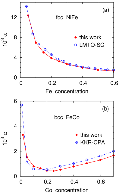
Figure 3: (Color online) The calculated concentration dependences of the Gilbert damping parameter $\alpha$ for random fcc NiFe (a) and bcc FeCo (b) alloys. The results of this work are marked by the full diamonds, whereas the open circles depict the results of other approaches: the LMTO supercell (LMTO-SC) technique Starikov et al. (2010) and the KKR-CPA method. Mankovsky et al. (2013)

III.2 Binary fcc and bcc solid solutions

The developed theory has been applied to random binary alloys of $3d$ transition elements Fe, Co, and Ni, namely, to the fcc NiFe and bcc FeCo alloys. The most important results, including a comparison to other existing ab initio techniques, are summarized in Fig. 3. One can see a good agreement of the calculated concentration trends of the Gilbert damping parameter $\alpha=\alpha_{xx}=\alpha_{yy}$ with the results of an LMTO-supercell approach Starikov et al. (2010) and of the KKR-CPA method. Mankovsky et al. (2013) The decrease of $\alpha$ with increasing Fe content in the concentrated NiFe alloys can be related to the increasing alloy magnetization Starikov et al. (2010) and to the decreasing strength of the SO-interaction, Sakuma (2012) whereas the behavior in the dilute limit can be explained by intraband scattering due to Fe impurities. Gilmore et al. (2007); Kamberský (2007); Gilmore et al. (2008) In the case of the FeCo system, the minimum of $\alpha$ around 20% Co, which is also observed in room-temperature experiments, Oogane et al. (2006); Schreiber et al. (1995) is related primarily to a similar concentration trend of the density of states at the Fermi energy, Mankovsky et al. (2013) though the maximum of the magnetization at roughly the same alloy composition Turek et al. (1994) might partly contribute as well.

Table 1: Comparison of the Gilbert damping parameter $\alpha$ for the fcc Ni₈₀Fe₂₀ random alloy (Permalloy) calculated by the present approach and by other techniques using the CPA or supercells (SC). The last column displays the coherent part $\alpha^{\rm coh}$ of the total damping parameter according to Eq. (11). The experimental value corresponds to room temperature.

Method	$\alpha$	$\alpha^{\rm coh}$
This work, $\varepsilon=10^{-5}$ Ry	$4.9\times 10^{-3}$	1.76
This work, $\varepsilon=10^{-6}$ Ry	$3.9\times 10^{-3}$	1.76
KKR-CPA	$4.2\times 10^{-3}$
LMTO-CPA	$3.5\times 10^{-3}$
LMTO-SC	$4.6\times 10^{-3}$
Experiment	$8\times 10^{-3}$

A more detailed comparison of all ab initio results is presented in Table 1 for the fcc Ni₈₀Fe₂₀ random alloy (Permalloy). The differences in the values of $\alpha$ from the different techniques can be ascribed to various theoretical features and numerical details employed, such as the simplified treatment of the SO-interaction in Ref. Sakuma, 2012 instead of the fully relativistic description, or the use of supercells in Ref. Starikov et al., 2010 instead of the CPA. Taking into account that calculated residual resistivities for this alloy span a wide interval between 2 $\mu\Omega$cm, see Ref. Banhart et al., 1997; Turek et al., 2012a, and 3.5 $\mu\Omega$cm, see Ref. Starikov et al., 2010, one can consider the scatter of the calculated values of $\alpha$ in Table 1 as little important. The theoretical values of $\alpha$ are smaller systematically than the measured values, typically by a factor of two. This discrepancy might be partly due to the effects of finite temperatures as well as due to additional structural defects of real samples.

A closer look at the theoretical results reveals that the total damping parameters $\alpha$ are appreciably smaller than the magnitudes of their coherent and vertex parts, see Table 1 for the case of Permalloy. This is in agreement with the results of the model study in Section II.1; similar conclusions about the importance of the vertex corrections have been done with the XC-induced torques in other CPA-based studies. Ebert et al. (2011a); Mankovsky et al. (2013); Sakuma (2015b) The present results prove that this unpleasant feature of the nonlocal torques does not represent a serious obstacle in obtaining reliable values of the Gilbert damping parameter in random alloys. We note that the vertex corrections can be negligible in approaches employing the SO-induced torques, at least for systems with the SO splittings much weaker than the XC splittings, Kamberský (2007) such as the binary ferromagnetic alloys of $3d$ transition metals, Sakuma (2015b) see also Section II.1.

III.3 Pure iron with a model disorder

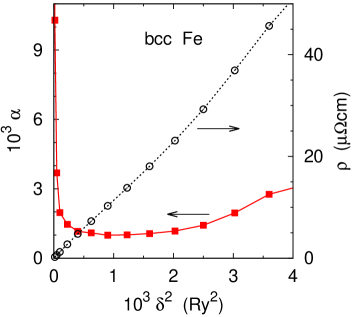
Figure 4: (Color online) The calculated Gilbert damping parameter $\alpha$ (full squares) and the residual resistivity $\rho$ (open circles) of pure bcc iron as functions of $\delta^{2}$, where $\delta$ is the strength of a model atomic-level disorder.

As it has been mentioned in Section I, the Gilbert damping of pure ferromagnetic metals exhibits non-trivial temperature dependences, which have been reproduced by means of ab initio techniques with various levels of sophistication. Gilmore et al. (2007); Kamberský (2007); Liu et al. (2011); Ebert et al. (2015) In this study, we have simulated the effect of finite temperatures by introducing static fluctuations of the one-particle potential. The adopted model of atomic-level disorder assumes that random spin-independent shifts $\pm\delta$, constant inside each atomic sphere and occurring with probabilities 50% of both signs, are added to the nonrandom selfconsistent potential obtained at zero temperature. The Fermi energy is kept frozen, equal to its selfconsistent zero-temperature value. This model can be easily treated in the CPA; the resulting Gilbert damping parameter $\alpha$ of pure bcc Fe as a function of the potential shift $\delta$ is plotted in Fig. 4.

The calculated dependence $\alpha(\delta)$ is nonmonotonic, with a minimum at $\delta\approx 30$ mRy. This trend is in a qualitative agreement with trends reported previously by other authors, who employed phenomenological models of the electron lifetime Gilmore et al. (2007); Kamberský (2007) as well as models for phonons and magnons. Liu et al. (2011); Ebert et al. (2015) The origin of the nonmonotonic dependence $\alpha(\delta)$ has been identified on the basis of the band structure of the ferromagnetic system as an interplay between the intraband contributions to $\alpha$, dominating for small values of $\delta$, and the interband contributions, dominating for large values of $\delta$. Sinova et al. (2004); Gilmore et al. (2007); Kamberský (2007) Since the present CPA-based approach does not use any bands, we cannot perform a similar analysis.

The obtained minimum value of the Gilbert damping, $\alpha_{\rm min}\approx 10^{-3}$ (Fig. 4), agrees reasonably well with the values obtained by the authors of Ref. Gilmore et al., 2007; Kamberský, 2007; Liu et al., 2011; Ebert et al., 2015. This agreement indicates that the atomic-level disorder employed here is equivalent to a phenomenological lifetime broadening. For a rough quantitative estimation of the temperature effect, one can employ the calculated resistivity $\rho$ of the model, which increases essentially linearly with $\delta^{2}$, see Fig. 4. Since the metallic resistivity due to phonons increases linearly with the temperature $T$ (for temperatures not much smaller than the Debye temperature), one can assume a proportionality between $\delta^{2}$ and $T$. The resistivity of bcc iron at the Curie temperature $T_{\rm C}=1044$ K due to lattice vibrations can be estimated around 35 $\mu\Omega$cm, Ebert et al. (2015); Weiss and Marotta (1959) which sets an approximate temperature scale to the data plotted in Fig. 4. However, a more accurate description of the temperature dependence of the Gilbert damping parameter cannot be obtained, mainly due to the neglected true atomic displacements and the noncollinearity of magnetic moments (magnons). Ebert et al. (2015)

III.4 FePt alloys with a partial long-range order

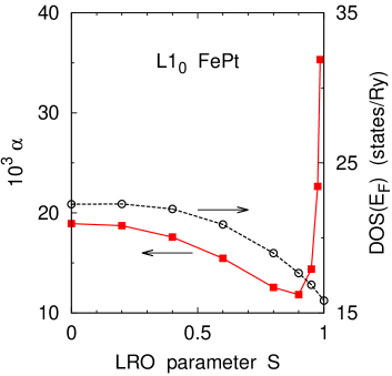
Figure 5: (Color online) The calculated Gilbert damping parameter $\alpha$ (full squares) and the total DOS (per formula unit) at the Fermi energy (open circles) of stoichiometric L1₀ FePt alloys as functions of the LRO parameter $S$.

Since important ferromagnetic materials include ordered alloys, we address here the Gilbert damping in stoichiometric FePt alloys with L1₀ atomic long-range order (LRO). Their transport properties Kudrnovský et al. (2014) and the damping parameter Sakuma (2012) have recently been studied by means of the TB-LMTO method in dependence on a varying degree of the LRO. These fcc-based systems contain two sublattices with respective occupations Fe_1-yPt_y and Pt_1-yFe_y where $y$ ($0\leq y\leq 0.5$) denotes the concentration of antisite atoms. The LRO parameter $S$ ($0\leq S\leq 1$) is then defined as $S=1-2y$, so that $S=0$ corresponds to the random fcc alloy and $S=1$ corresponds to the perfectly ordered L1₀ structure.

The resulting Gilbert damping parameter is displayed in Fig. 5 as a function of $S$. The obtained trend with a broad maximum at $S=0$ and a minimum around $S=0.9$ agrees very well with the previous result. Sakuma (2012) The values of $\alpha$ in Fig. 5 are about 10% higher than those in Ref. Sakuma, 2012, which can be ascribed to the fully relativistic treatment in the present study in contrast to a simplified treatment of the SO interaction in Ref. Sakuma, 2012. The Gilbert damping in the FePt alloys is an order of magnitude stronger than in the alloys of $3d$ elements (Section III.2) owing to the stronger SO interaction of Pt atoms. The origin of the slow decrease of $\alpha$ with increasing $S$ (for $0\leq S\leq 0.9$) can be explained by the decreasing total density of states (DOS) at the Fermi energy, see Fig. 5, which represents an analogy to a similar correlation observed, e.g., for bcc FeCo alloys. Mankovsky et al. (2013)

All calculated values of $\alpha$ shown in Fig. 5, corresponding to $0\leq S\leq 0.985$, are appreciably smaller than the measured one which amounts to $\alpha\approx 0.06$ reported for a thin L1₀ FePt epitaxial film. Mizukami et al. (2011) The high measured value of $\alpha$ might be thus explained by the present calculations by assuming a very small concentration of antisites in the prepared films, which does not seem too realistic. Another potential source of the discrepancy lies in the thin-film geometry used in the experiment. Moreover, the divergence of $\alpha$ in the limit of $S\to 1$ (Fig. 5) illustrates a general shortcoming of approaches based on the torque-correlation formula (2), since the zero-temperature Gilbert damping parameter of a pure ferromagnet should remain finite. A correct treatment of this case, including the dilute limit of random alloys (Fig. 3), must take into account the full interacting susceptibility in the presence of SO interaction. Garate and MacDonald (2009a); Korenman and Prange (1972) Pilot ab initio studies in this direction have recently appeared for nonrandom systems; dos Santos Dias et al. (2015); Lounis et al. (2015) however, their extension to disordered systems goes far beyond the scope of this work.

IV Conclusions

We have introduced nonlocal torques as an alternative to the usual local torque operators entering the torque-correlation formula for the Gilbert damping tensor. Within the relativistic TB-LMTO-ASA method, this idea leads to effective nonlocal torques as non-site-diagonal and spin-independent matrices. For substitutionally disordered alloys, the nonlocal torques are nonrandom, which allows one to develop an internally consistent theory in the CPA. The CPA-vertex corrections proved indispensable for an exact equivalence of the nonlocal nonrandom torques with their local random counterparts. The concept of the nonlocal torques is not limited to the LMTO method and its formulation both in a semiempirical TB theory and in the KKR theory is straightforward.

The numerical implementation and the results for binary solid solutions show that the total Gilbert damping parameters from the nonlocal torques are much smaller than magnitudes of the coherent parts and of the vertex corrections. Nevertheless, the total damping parameters for the studied NiFe, FeCo and FePt alloys compare quantitatively very well with results of other ab initio techniques, Starikov et al. (2010); Sakuma (2012); Mankovsky et al. (2013) which indicates a fair numerical stability of the developed theory.

The performed numerical study of the Gilbert damping in pure bcc iron as a function of an atomic-level disorder yields a nonmonotonic dependence in a qualitative agreement with the trends consisting of the conductivity-like and resistivity-like regions, obtained from a phenomenological quasiparticle lifetime broadening Sinova et al. (2004); Gilmore et al. (2007); Kamberský (2007) or from the temperature-induced frozen phonons Liu et al. (2011); Mankovsky et al. (2013) and magnons. Ebert et al. (2015) Future studies should clarify the applicability of the introduced nonlocal torques to a full quantitative description of the finite-temperature behavior as well as to other torque-related phenomena, such as the spin-orbit torques due to applied electric fields. Manchon and Zhang (2009); Freimuth et al. (2014)

Appendix A Torque correlation formula in a matrix representation

In this Appendix, evaluation of the Kubo-Greenwood expression for the torque-correlation formula (2) is discussed in the case of the XC-induced torque operators using matrix representations of all operators in an orthonormal basis that varies due to the varying direction of the XC field. All operators are denoted by a hat, in order to be distinguished from matrices representing these operators in the chosen basis. Let us consider a one-particle Hamiltonian ${\hat{H}}={\hat{H}}(\theta_{1},\theta_{2})$ depending on two real variables $\theta_{j}$, $j=1,2$, and let us denote ${\hat{T}}^{(j)}(\theta_{1},\theta_{2})=\partial{\hat{H}}(\theta_{1},\theta_{2})/\partial\theta_{j}$. In our case, the variables $\theta_{j}$ play the role of rotation angles and the operators ${\hat{T}}^{(j)}$ are the corresponding torques. Let us denote the resolvents of ${\hat{H}}(\theta_{1},\theta_{2})$ at the Fermi energy as ${\hat{G}}_{\pm}(\theta_{1},\theta_{2})$ and let us consider a special linear response coefficient (arguments $\theta_{1}$ and $\theta_{2}$ are omitted here and below for brevity)

$$c = {\rm Tr}\{{\hat{T}}^{(1)}({\hat{G}}_{+}-{\hat{G}}_{-}){\hat{T}}^{(2)}({\hat{G}}_{+}-{\hat{G}}_{-})\}$$

$$= {\rm Tr}\{(\partial{\hat{H}}/\partial\theta_{1})({\hat{G}}_{+}-{\hat{G}}_{-})(\partial{\hat{H}}/\partial\theta_{2})({\hat{G}}_{+}-{\hat{G}}_{-})\}.$$

This torque-correlation coefficient equals the Gilbert damping parameter (2) with the prefactor $(-\alpha_{0})$ suppressed. For its evaluation, we introduce an orthonormal basis $|\chi_{m}(\theta_{1},\theta_{2})\rangle$ and represent all operators in this basis. This leads to matrices $H(\theta_{1},\theta_{2})=\{H_{mn}(\theta_{1},\theta_{2})\}$, $G_{\pm}(\theta_{1},\theta_{2})=\{(G_{\pm})_{mn}(\theta_{1},\theta_{2})\}$ and $T^{(j)}(\theta_{1},\theta_{2})=\{T^{(j)}_{mn}(\theta_{1},\theta_{2})\}$, where

$$H_{mn} = \langle\chi_{m}|{\hat{H}}|\chi_{n}\rangle,\qquad(G_{\pm})_{mn}=\langle\chi_{m}|{\hat{G}}_{\pm}|\chi_{n}\rangle,$$

$$T^{(j)}_{mn} = \langle\chi_{m}|{\hat{T}}^{(j)}|\chi_{n}\rangle=\langle\chi_{m}|\partial{\hat{H}}/\partial\theta_{j}|\chi_{n}\rangle,$$ (15)

and, consequently, to the response coefficient (A) expressed by using the matrices (15) as

$$c={\rm Tr}\{T^{(1)}(G_{+}-G_{-})T^{(2)}(G_{+}-G_{-})\}.$$ (16)

However, in evaluation of the last expression, attention has to be paid to the difference between the matrix $T^{(j)}(\theta_{1},\theta_{2})$ and the partial derivative of the matrix $H(\theta_{1},\theta_{2})$ with respect to $\theta_{j}$. This difference follows from the identity ${\hat{H}}=\sum_{mn}|\chi_{m}\rangle H_{mn}\langle\chi_{n}|$, which yields

$$T^{(j)}_{mn} = \partial H_{mn}/\partial\theta_{j}+\sum_{k}\langle\chi_{m}|\partial\chi_{k}/\partial\theta_{j}\rangle H_{kn}$$ (17)

$$+\sum_{k}H_{mk}\langle\partial\chi_{k}/\partial\theta_{j}|\chi_{n}\rangle,$$

where we employed the orthogonality relations $\langle\chi_{m}(\theta_{1},\theta_{2})|\chi_{n}(\theta_{1},\theta_{2})\rangle=\delta_{mn}$. Their partial derivatives yield

$$\langle\chi_{m}|\partial\chi_{n}/\partial\theta_{j}\rangle=-\langle\partial\chi_{m}/\partial\theta_{j}|\chi_{n}\rangle\equiv Q^{(j)}_{mn},$$ (18)

where we introduced elements of matrices $Q^{(j)}=\{Q^{(j)}_{mn}\}$ for $j=1,2$. Note that the matrices $Q^{(j)}(\theta_{1},\theta_{2})$ reflect explicitly the dependence of the basis vectors $|\chi_{m}(\theta_{1},\theta_{2})\rangle$ on $\theta_{1}$ and $\theta_{2}$. The relation (17) between the matrices $T^{(j)}$ and $\partial H/\partial\theta_{j}$ can be now rewritten compactly as

$$T^{(j)}=\partial H/\partial\theta_{j}+[Q^{(j)},H].$$ (19)

Since the last term has a form of a commutator with the Hamiltonian matrix $H$, the use of Eq. (19) in the formula (16) leads to the final matrix expression for the torque correlation,

$$c={\rm Tr}\{(\partial H/\partial\theta_{1})(G_{+}-G_{-})(\partial H/\partial\theta_{2})(G_{+}-G_{-})\}.$$ (20)

The equivalence of Eqs. (16) and (20) rests on the rules $[Q^{(j)},H]=[E_{\rm F}-H,Q^{(j)}]$ and $(E_{\rm F}-H)(G_{+}-G_{-})=(G_{+}-G_{-})(E_{\rm F}-H)=0$ and on the cyclic invariance of the trace. It is also required that the matrices $Q^{(j)}$ are compatible with periodic boundary conditions used in calculations of extended systems, which is obviously the case for angular variables $\theta_{j}$ related to the global changes (uniform rotations) of the magnetization direction.

The obtained result means that the original response coefficient (A) involving the torques as angular derivatives of the Hamiltonian can be expressed solely by using matrix elements of the Hamiltonian in an angle-dependent basis; the angular dependence of the basis vectors does not enter explicitly the final torque-correlation formula (20).

Appendix B LMTO Hamiltonian of a ferromagnet with a tilted magnetic field

Here we sketch a derivation of the fully relativistic LMTO Hamiltonian matrix for a ferromagnet with the XC-field direction tilted from a reference direction along an easy axis. The derivation rests on the form of the Kohn-Sham-Dirac Hamiltonian in the LMTO-ASA method. Solovyev et al. (1991); Shick et al. (1996); Turek et al. (1997) The symbols with superscript $0$ refer to the reference system, the symbols without this superscript refer to the system with the tilted XC field. The operators (Hamiltonians, rotation operators) are denoted by symbols with a hat. The spin-dependent parts of the ASA potentials due to the XC fields are rigidly rotated while the spin-independent parts are unchanged, in full analogy to the approach employed in the relativistic KKR method. Ebert et al. (2011a); Mankovsky et al. (2013)

The ASA-Hamiltonians of both systems are given by lattice sums ${\hat{H}}^{0}=\sum_{\bf R}{\hat{H}}^{0}_{\bf R}$ and ${\hat{H}}=\sum_{\bf R}{\hat{H}}_{\bf R}$, where the individual site-contributions are coupled mutually by ${\hat{H}}_{\bf R}={\hat{U}}_{\bf R}{\hat{H}}^{0}_{\bf R}{\hat{U}}^{+}_{\bf R}$, where ${\hat{U}}_{\bf R}$ denotes the unitary operator of a rotation (in the orbital and spin space) around the ${\bf R}$th lattice site which brings the local XC field from its reference direction into the tilted one. Let $|\phi^{0}_{{\bf R}\Lambda}\rangle$ and $|{\dot{\phi}}^{0}_{{\bf R}\Lambda}\rangle$ denote, respectively, the phi and phi-dot orbitals of the reference Hamiltonian ${\hat{H}}^{0}_{\bf R}$, then

$$|\phi_{{\bf R}\Lambda}\rangle={\hat{U}}_{\bf R}|\phi^{0}_{{\bf R}\Lambda}\rangle,\qquad|{\dot{\phi}}_{{\bf R}\Lambda}\rangle={\hat{U}}_{\bf R}|{\dot{\phi}}^{0}_{{\bf R}\Lambda}\rangle$$ (21)

define the phi and phi-dot orbitals of the Hamiltonian ${\hat{H}}_{\bf R}$. The orbital index $\Lambda$ labels all linearly independent solutions (regular at the origin) of the spin-polarized relativistic single-site problem; the detailed structure of $\Lambda$ can be found elsewhere. Solovyev et al. (1991); Shick et al. (1996); Turek et al. (1997) Let us introduce further the well-known empty-space solutions $|K^{\infty,0}_{{\bf R}N}\rangle$ (extending over the whole real space), $|K^{\mathrm{int},0}_{{\bf R}N}\rangle$ (extending over the interstitial region), and $|K^{0}_{{\bf R}N}\rangle$ and $|J^{0}_{{\bf R}N}\rangle$ (both truncated outside the ${\bf R}$th sphere), needed for the definition of the LMTOs of the reference system. Andersen and Jepsen (1984); Andersen et al. (1985, 1986) Their index $N$, which defines the spin-spherical harmonics of the large component of each solution, can be taken either in the nonrelativistic $(\ell ms)$ form or in its relativistic $(\kappa\mu)$ counterpart. We define further

$$|Z_{{\bf R}N}\rangle={\hat{U}}_{\bf R}|Z^{0}_{{\bf R}N}\rangle\qquad\mathrm{for}\ \,Z=K^{\infty},\,K,\,J.$$ (22)

Isotropy of the empty space guarantees relations (for $Z=K^{\infty}$, $K$, $J$)

$$|Z_{{\bf R}N}\rangle = \sum_{N^{\prime}}|Z^{0}_{{\bf R}N^{\prime}}\rangle U_{N^{\prime}N},$$

$$|Z^{0}_{{\bf R}N}\rangle = \sum_{N^{\prime}}|Z_{{\bf R}N^{\prime}}\rangle U^{+}_{N^{\prime}N},$$ (23)

where $U=\{U_{N^{\prime}N}\}$ denotes a unitary matrix representing the rotation in the space of spin-spherical harmonics and where $U^{+}_{N^{\prime}N}\equiv(U^{+})_{N^{\prime}N}=(U_{NN^{\prime}})^{\ast}=(U^{-1})_{N^{\prime}N}$; the matrix $U$ is the same for all lattice sites ${\bf R}$ since we consider only uniform rotations of the XC-field direction inside the ferromagnet. The expansion theorem for the envelope orbital $|K^{\infty,0}_{{\bf R}N}\rangle$ is

$$|K^{\infty,0}_{{\bf R}N}\rangle = |K^{\mathrm{int},0}_{{\bf R}N}\rangle+|K^{0}_{{\bf R}N}\rangle$$ (24)

$$-\sum_{{\bf R}^{\prime}N^{\prime}}|J^{0}_{{\bf R}^{\prime}N^{\prime}}\rangle S^{0}_{{\bf R}^{\prime}N^{\prime},{\bf R}N},$$

where $S^{0}_{{\bf R}^{\prime}N^{\prime},{\bf R}N}$ denote elements of the canonical structure-constant matrix (with vanishing on-site elements, $S^{0}_{{\bf R}N^{\prime},{\bf R}N}=0$) of the reference system. The use of relations (23) in the expansion (24) together with an abbreviation

$$|K^{\mathrm{int}}_{{\bf R}N}\rangle=\sum_{N^{\prime}}|K^{\mathrm{int},0}_{{\bf R}N^{\prime}}\rangle U_{N^{\prime}N}$$ (25)

yields the expansion of the envelope orbital $|K^{\infty}_{{\bf R}N}\rangle$ as

$$|K^{\infty}_{{\bf R}N}\rangle = |K^{\mathrm{int}}_{{\bf R}N}\rangle+|K_{{\bf R}N}\rangle$$ (26)

$$-\sum_{{\bf R}^{\prime}N^{\prime}}|J_{{\bf R}^{\prime}N^{\prime}}\rangle(U^{+}S^{0}U)_{{\bf R}^{\prime}N^{\prime},{\bf R}N},$$

where $U$ and $U^{+}$ denote site-diagonal matrices with elements $U_{{\bf R}^{\prime}N^{\prime},{\bf R}N}=\delta_{{\bf R}^{\prime}{\bf R}}U_{N^{\prime}N}$ and $(U^{+})_{{\bf R}^{\prime}N^{\prime},{\bf R}N}=\delta_{{\bf R}^{\prime}{\bf R}}U^{+}_{N^{\prime}N}$. Note the same form of expansions (24) and (26), with the orbitals $|Z^{0}_{{\bf R}N}\rangle$ replaced by the rotated orbitals $|Z_{{\bf R}N}\rangle$ ($Z=K^{\infty},K,J$), with the interstitial parts $|K^{\mathrm{int},0}_{{\bf R}N}\rangle$ replaced by their linear combinations $|K^{\mathrm{int}}_{{\bf R}N}\rangle$, and with the structure-constant matrix $S^{0}$ replaced by the product $U^{+}S^{0}U$.

The non-orthogonal LMTO $|\chi^{0}_{{\bf R}N}\rangle$ for the reference system is obtained from the expansion (24), in which all orbitals $|K^{0}_{{\bf R}N}\rangle$ and $|J^{0}_{{\bf R}N}\rangle$ are replaced by linear combinations of $|\phi^{0}_{{\bf R}\Lambda}\rangle$ and $|{\dot{\phi}}^{0}_{{\bf R}\Lambda}\rangle$. A similar replacement of the orbitals $|K_{{\bf R}N}\rangle$ and $|J_{{\bf R}N}\rangle$ by linear combinations of $|\phi_{{\bf R}\Lambda}\rangle$ and $|{\dot{\phi}}_{{\bf R}\Lambda}\rangle$ in the expansion (26) yields the non-orthogonal LMTO $|\chi_{{\bf R}N}\rangle$ for the system with the tilted XC field. The coefficients in these linear combinations—obtained from conditions of continuous matching at the sphere boundaries and leading directly to the LMTO potential parameters—are identical for both systems, as follows from the rotation relations (21) and (22). For these reasons, the only essential difference between both systems in the construction of the non-orthogonal and orthogonal LMTOs (and of the accompanying Hamiltonian and overlap matrices in the ASA) is due to the difference between the matrices $S^{0}$ and $U^{+}S^{0}U$.

As a consequence, the LMTO Hamiltonian matrix in the orthogonal LMTO representation for the system with a tilted magnetization is easily obtained from that for the reference system, Eq. (6), and it is given by

$$H=C+(\sqrt{\Delta})^{+}U^{+}SU(1-\gamma U^{+}SU)^{-1}\sqrt{\Delta},$$ (27)

where the $C$, $\sqrt{\Delta}$ and $\gamma$ are site-diagonal matrices of the potential parameters of the reference system and where we suppressed the superscript $0$ at the structure-constant matrix $S$ of the reference system. Note that the dependence of $H$ on the XC-field direction is contained only in the similarity transformation $U^{+}SU$ of the original structure-constant matrix $S$ generated by the rotation matrix $U$. For the rotation by an angle $\theta$ around an axis along a unit vector ${\bf n}$, the rotation matrix is given by $U(\theta)=\exp(-{\rm i}{\bf n}\cdot{\bf J}\theta)$, where the site-diagonal matrices ${\bf J}\equiv({\cal J}^{x},{\cal J}^{y},{\cal J}^{z})$ with matrix elements ${\cal J}^{\mu}_{{\bf R}^{\prime}N^{\prime},{\bf R}N}=\delta_{{\bf R}^{\prime}{\bf R}}{\cal J}^{\mu}_{N^{\prime}N}$ ($\mu=x,y,z$) reduce to usual matrices of the total (orbital plus spin) angular momentum operator. The limit of small $\theta$ yields $U(\theta)\approx 1-{\rm i}{\bf n}\cdot{\bf J}\theta$, which leads to the $\theta$-derivative of the Hamiltonian matrix (27) at $\theta=0$:

$$\partial H/\partial\theta={\rm i}(F^{+})^{-1}[{\bf n}\cdot{\bf J},S]F^{-1},$$ (28)

where we abbreviated $F=(\sqrt{\Delta})^{-1}(1-\gamma S)$ and $F^{+}=(1-S\gamma)[(\sqrt{\Delta})^{+}]^{-1}$. Since the structure-constant matrix $S$ is spin-independent, the total angular momentum operator ${\bf J}$ in (28) can be replaced by its orbital momentum counterpart ${\bf L}\equiv({\cal L}^{x},{\cal L}^{y},{\cal L}^{z})$, so that

$$\partial H/\partial\theta={\rm i}(F^{+})^{-1}[{\bf n}\cdot{\bf L},S]F^{-1}.$$ (29)

The relations (28) and (29) are used to derive the LMTO-ASA torque-correlation formula (8).

Appendix C Equivalence of the Gilbert damping in the CPA with local and nonlocal torques (Supplemental Material)

C.1 Introductory remarks

The problem of equivalence of the Gilbert damping tensor expressed with the local (loc) and nonlocal (nl) torques can be reduced to the problem of equivalence of these two expressions:

$$\alpha^{\rm loc} = \alpha_{0}\,{\rm Tr}\langle(g_{+}-g_{-})[P,K](g_{+}-g_{-})[P,K]\rangle$$ (30)

$$= \alpha_{0}\sum_{p=\pm}\sum_{q=\pm}{\rm sgn}(pq)\,{\rm Tr}\langle g_{p}[P,K]g_{q}[P,K]\rangle$$

$$= \alpha_{0}\sum_{p=\pm}\sum_{q=\pm}{\rm sgn}(pq)\beta^{\rm loc}_{pq},$$

and

$$\alpha^{\rm nl} = \alpha_{0}\,{\rm Tr}\langle(g_{+}-g_{-})[K,S](g_{+}-g_{-})[K,S]\rangle$$ (31)

$$= \alpha_{0}\sum_{p=\pm}\sum_{q=\pm}{\rm sgn}(pq)\,{\rm Tr}\langle g_{p}[K,S]g_{q}[K,S]\rangle$$

$$= \alpha_{0}\sum_{p=\pm}\sum_{q=\pm}{\rm sgn}(pq)\beta^{\rm nl}_{pq}.$$

The symbols ${\rm Tr}$ and $\langle\dots\rangle$ and the quantities $\alpha_{0}$, $g_{\pm}$, $P$ and $S$ have the same meaning as in the main text and the quantity $K$ substitutes any of the operators (matrices) ${\cal J}^{\mu}$ or ${\cal L}^{\mu}$. Note that owing to the symmetric nature of the original damping tensors, the analysis can be confined to scalar quantities $\alpha^{\rm loc}$ and $\alpha^{\rm nl}$ depending on a general site-diagonal nonrandom operator $K$. The choice of $K=K^{\mu}$ in (30) and (31) produces the diagonal elements of both tensors, whereas the choice of $K=K^{\mu}\pm K^{\nu}$ for $\mu\neq\nu$ leads to all off-diagonal elements. The quantities $\beta^{\rm loc}_{pq}$ and $\beta^{\rm nl}_{pq}$ are expressions of the form

$$\beta^{\rm loc} = {\rm Tr}\langle g^{1}(P^{1}K-KP^{2})g^{2}(P^{2}K-KP^{1})\rangle,$$

$$\beta^{\rm nl} = {\rm Tr}\langle g^{1}[K,S]g^{2}[K,S]\rangle,$$ (32)

where the $g^{1}$ and $g^{2}$ replace the $g_{p}$ and $g_{q}$, respectively. For an internal consistency of these and following expressions, we have also introduced $P^{1}=P^{2}=P$.

This supplement contains a proof of the equivalence of $\beta^{\rm loc}$ and $\beta^{\rm nl}$ and, consequently, of $\alpha^{\rm loc}$ and $\alpha^{\rm nl}$. The CPA-average in $\beta^{\rm nl}$ with a nonlocal nonrandom torque has been done using the theory by Velický Velický (1969) as worked out in detail within the present LMTO formalism by Carva et al. Carva et al. (2006) whereas the averaging in $\beta^{\rm loc}$ involving a local but random torque has been treated using the approach by Butler. Butler (1985)

C.2 Auxiliary quantities and relations

Since the necessary formulas of the CPA in multiorbital techniques Carva et al. (2006); Butler (1985) are little transparent, partly owing to the complicated indices of two-particle quantities, we employ here a formalism with the lattice-site index ${\bf R}$ kept but with all orbital indices suppressed.

The Hilbert space is a sum of mutually orthogonal subspaces of individual lattice sites ${\bf R}$; the corresponding projectors will be denoted by $\Pi_{\bf R}$. A number of relevant operators are site-diagonal, i.e., they can be written as $X=\sum_{\bf R}X_{\bf R}$, where the site contributions are given by $X_{\bf R}=\Pi_{\bf R}X=X\Pi_{\bf R}=\Pi_{\bf R}X\Pi_{\bf R}$. Such operators are, e.g., the random potential functions, $P^{j}=\sum_{\bf R}P^{j}_{\bf R}$, and the nonrandom coherent potential functions ${\cal P}^{j}=\sum_{\bf R}{\cal P}^{j}_{\bf R}$, where $j=1,2$. The operator $K$ in (32) is site-diagonal as well, but its site contributions $K_{\bf R}$ will not be used explicitly in the following.

Among the number of CPA-relations for single-particle properties, we will use the equation of motion for the average auxiliary Green’s functions ${\bar{g}}^{j}$ ($j=1,2$),

$${\bar{g}}^{j}({\cal P}^{j}-S)=({\cal P}^{j}-S){\bar{g}}^{j}=1,$$ (33)

as well as the definition of random single-site t-matrices $t^{j}_{\bf R}$ ($j=1,2$) with respect to the effective CPA-medium, given by

$$t^{j}_{\bf R}=(P^{j}_{\bf R}-{\cal P}^{j}_{\bf R})[1+{\bar{g}}^{j}(P^{j}_{\bf R}-{\cal P}^{j}_{\bf R})]^{-1}.$$ (34)

The operators $t^{j}_{\bf R}$ are site-diagonal, being non-zero only in the subspace of site ${\bf R}$. The last definition leads to identities

$$(1-t^{1}_{\bf R}\bar{g}^{1})P^{1}_{\bf R} = {\cal P}^{1}_{\bf R}+t^{1}_{\bf R}(1-\bar{g}^{1}{\cal P}^{1}_{\bf R}),$$

$$P^{2}_{\bf R}(1-\bar{g}^{2}t^{2}_{\bf R}) = {\cal P}^{2}_{\bf R}+(1-{\cal P}^{2}_{\bf R}\bar{g}^{2})t^{2}_{\bf R},$$ (35)

which will be employed below together with the CPA-selfconsistency conditions $\langle t^{j}_{\bf R}\rangle=0$ ($j=1,2$).

For the purpose of evaluation of the two-particle averages in (32), we introduce several nonrandom operators:

$$f^{12}=\bar{g}^{1}K-K\bar{g}^{2},\qquad\zeta^{12}=\bar{g}^{1}[K,S]\bar{g}^{2},$$ (36)

and a site-diagonal operator $\gamma^{12}=\sum_{\bf R}\gamma^{12}_{\bf R}$, where

$$\gamma^{12}={\cal P}^{1}K-K{\cal P}^{2},\qquad\gamma^{12}_{\bf R}={\cal P}^{1}_{\bf R}K-K{\cal P}^{2}_{\bf R}.$$ (37)

By interchanging the superscripts $1\leftrightarrow 2$ in (36) and (37), one can also get quantities $f^{21}$, $\zeta^{21}$, $\gamma^{21}$ and $\gamma^{21}_{\bf R}$; this will be implicitly understood in the relations below as well. The three operators $f^{12}$, $\zeta^{12}$ and $\gamma^{12}$ satisfy a relation

$$f^{12}+\zeta^{12}+\bar{g}^{1}\gamma^{12}\bar{g}^{2}=0,$$ (38)

which can be easily proved from their definitions (36) and (37) and from the equation of motion (33). Another quantity to be used in the following is a nonrandom site-diagonal operator $\vartheta^{12}$ related to the local torque and defined by

$$\vartheta^{12}_{\bf R} = \langle(1-t^{1}_{\bf R}\bar{g}^{1})(P^{1}_{\bf R}K-KP^{2}_{\bf R})(1-\bar{g}^{2}t^{2}_{\bf R})\rangle,$$

$$\vartheta^{12} = \sum_{\bf R}\vartheta^{12}_{\bf R}.$$ (39)

Its site contributions can be rewritten explicitly as

$$\vartheta^{12}_{\bf R}=\gamma^{12}_{\bf R}+\langle t^{1}_{\bf R}(f^{12}+\bar{g}^{1}\gamma^{12}_{\bf R}\bar{g}^{2})t^{2}_{\bf R}\rangle.$$ (40)

The last relation follows from the definition (39), from the identities (35) and from the CPA-selfconsistency conditions. Moreover, the site contributions $\vartheta^{12}_{\bf R}$ and $\gamma^{12}_{\bf R}$ satisfy a sum rule

$$\gamma^{12}_{\bf R}={\sum_{{\bf R}^{\prime}}}^{\prime}\langle t^{1}_{\bf R}\bar{g}^{1}\gamma^{12}_{{\bf R}^{\prime}}\bar{g}^{2}t^{2}_{\bf R}\rangle+\langle t^{1}_{\bf R}\zeta^{12}t^{2}_{\bf R}\rangle+\vartheta^{12}_{\bf R},$$ (41)

where the prime at the sum excludes the term with ${\bf R}^{\prime}={\bf R}$. This sum rule can be proved by using the definitions of $\zeta^{12}$ (36) and $\gamma^{12}_{\bf R}$ (37) and by employing the previous relation for $\vartheta^{12}_{\bf R}$ (40) and the equation of motion (33).

The treatment of two-particle quantities requires the use of a direct product $a\otimes b$ of two operators $a$ and $b$. This is equivalent to the concept of a superoperator, i.e., a linear mapping defined on the vector space of all linear operators. In this supplement, superoperators are denoted by an overhat, e.g., $\hat{m}$. In the present formalism, the direct product of two operators $a$ and $b$ can be identified with a superoperator $\hat{m}=a\otimes b$, which induces a mapping

$$x\mapsto\hat{m}x=(a\otimes b)x=axb,$$ (42)

where $x$ denotes an arbitrary usual operator. This definition leads, e.g., to a superoperator multiplication rule

$$(a\otimes b)(c\otimes d)=(ac)\otimes(db).$$ (43)

In the CPA, the most important superoperators are

$$\hat{w}^{12}=\sum_{\bf R}\langle t^{1}_{\bf R}\otimes t^{2}_{\bf R}\rangle$$ (44)

and

$$\hat{\chi}^{12}={\sum_{{\bf R}{\bf R}^{\prime}}}^{\prime}\Pi_{\bf R}\bar{g}^{1}\Pi_{{\bf R}^{\prime}}\otimes\Pi_{{\bf R}^{\prime}}\bar{g}^{2}\Pi_{\bf R}$$ (45)

where the prime at the double sum excludes the terms with ${\bf R}={\bf R}^{\prime}$. The quantity $\hat{w}^{12}$ represents the irreducible CPA-vertex and the quantity $\hat{\chi}^{12}$ corresponds to a restricted two-particle propagator with excluded on-site terms. By using these superoperators, the previous sum rule (41) can be rewritten compactly as

$$(\hat{1}-\hat{w}^{12}\hat{\chi}^{12})\gamma^{12}=\hat{w}^{12}\zeta^{12}+\vartheta^{12},$$ (46)

where $\hat{1}=1\otimes 1$ denotes the unit superoperator.

Let us introduce finally a symbol $\{x\,;y\}$, where $x$ and $y$ are arbitrary operators, which is defined by

$$\{x\,;y\}={\rm Tr}(xy).$$ (47)

This symbol is symmetric, $\{x\,;y\}=\{y\,;x\}$, linear in both arguments and it satisfies the rule

$$\{(a\otimes b)x\,;y\}=\{x\,;(b\otimes a)y\},$$ (48)

which follows from the cyclic invariance of the trace. An obvious consequence of this rule are relations

$$\{\hat{w}^{12}x\,;y\} = \{x\,;\hat{w}^{21}y\},$$

$$\{\hat{\chi}^{12}x\,;y\} = \{x\,;\hat{\chi}^{21}y\},$$ (49)

where $\hat{w}^{21}$ and $\hat{\chi}^{21}$ are defined by (44) and (45) with the superscript interchange $1\leftrightarrow 2$.

C.3 Expression with the nonlocal torque

The configuration averaging in $\beta^{\rm nl}$ (32), which contains the nonrandom operator $[K,S]$, leads to two terms

$$\beta^{\rm nl}=\beta^{\rm nl,coh}+\beta^{\rm nl,vc},$$ (50)

where the coherent part is given by

$$\beta^{\rm nl,coh}={\rm Tr}\{\bar{g}^{1}[K,S]\bar{g}^{2}[K,S]\}$$ (51)

and the vertex corrections can be compactly written as Carva et al. (2006)

$$\beta^{\rm nl,vc}=\{(\hat{1}-\hat{w}^{12}\hat{\chi}^{12})^{-1}\hat{w}^{12}\zeta^{12}\,;\zeta^{21}\},$$ (52)

with all symbols and quantities defined in the previous section. The coherent part can be written as a sum of four terms,

$$\beta^{\rm nl,coh} = \beta^{\rm nl,coh}_{A}+\beta^{\rm nl,coh}_{B}+\beta^{\rm nl,coh}_{C}+\beta^{\rm nl,coh}_{D},$$

$$\beta^{\rm nl,coh}_{A} = {\rm Tr}\{S\bar{g}^{1}KS\bar{g}^{2}K\},$$

$$\beta^{\rm nl,coh}_{B} = {\rm Tr}\{\bar{g}^{1}SK\bar{g}^{2}SK\},$$

$$\beta^{\rm nl,coh}_{C} = -{\rm Tr}\{\bar{g}^{1}KS\bar{g}^{2}SK\},$$

$$\beta^{\rm nl,coh}_{D} = -{\rm Tr}\{S\bar{g}^{1}SK\bar{g}^{2}K\},$$ (53)

which can be further modified using the equation of motion (33) and its consequences, e.g., $S{\bar{g}}^{j}={\cal P}^{j}{\bar{g}}^{j}-1$. For the first term $\beta^{\rm nl,coh}_{A}$, one obtains:

$$\beta^{\rm nl,coh}_{A} = {\rm Tr}\{{\cal P}^{1}\bar{g}^{1}K{\cal P}^{2}\bar{g}^{2}K\}+{\rm Tr}\{KK\}$$ (54)

$${}-{\rm Tr}\{K{\cal P}^{2}\bar{g}^{2}K\}-{\rm Tr}\{{\cal P}^{1}\bar{g}^{1}KK\}.\quad$$

The last three terms do not contribute to the sum over four pairs of indices $(p,q)$, where $p,q\in\{+,-\}$, in Eq. (31). For this reason, they can be omitted for the present purpose, which yields expressions

$${\tilde{\beta}}^{\rm nl,coh}_{A} = {\rm Tr}\{{\cal P}^{1}\bar{g}^{1}K{\cal P}^{2}\bar{g}^{2}K\},$$

$${\tilde{\beta}}^{\rm nl,coh}_{B} = {\rm Tr}\{\bar{g}^{1}{\cal P}^{1}K\bar{g}^{2}{\cal P}^{2}K\},$$ (55)

where the second relation is obtained in the same way from the original term $\beta^{\rm nl,coh}_{B}$. A similar approach can be applied to the third term $\beta^{\rm nl,coh}_{C}$, which yields

$$\beta^{\rm nl,coh}_{C} = -{\rm Tr}\{\bar{g}^{1}K{\cal P}^{2}\bar{g}^{2}{\cal P}^{2}K\}$$ (56)

$${}+{\rm Tr}\{\bar{g}^{1}K{\cal P}^{2}K\}+{\rm Tr}\{\bar{g}^{1}KSK\}.\quad$$

The last term does not contribute to the sum over four pairs $(p,q)$ in Eq. (31), which leads to expressions

$${\tilde{\beta}}^{\rm nl,coh}_{C} = {\rm Tr}\{\bar{g}^{1}K{\cal P}^{2}K\}-{\rm Tr}\{\bar{g}^{1}K{\cal P}^{2}\bar{g}^{2}{\cal P}^{2}K\},$$

$${\tilde{\beta}}^{\rm nl,coh}_{D} = {\rm Tr}\{{\cal P}^{1}K\bar{g}^{2}K\}-{\rm Tr}\{{\cal P}^{1}\bar{g}^{1}{\cal P}^{1}K\bar{g}^{2}K\},\qquad$$ (57)

where the second relation is obtained in the same way from the original term $\beta^{\rm nl,coh}_{D}$. The sum of all four contributions in (55) and (57) yields

$${\tilde{\beta}}^{\rm nl,coh} = {\tilde{\beta}}^{\rm nl,coh}_{A}+{\tilde{\beta}}^{\rm nl,coh}_{B}+{\tilde{\beta}}^{\rm nl,coh}_{C}+{\tilde{\beta}}^{\rm nl,coh}_{D}$$ (58)

$$= {\rm Tr}\{\bar{g}^{1}K{\cal P}^{2}K\}+{\rm Tr}\{{\cal P}^{1}K\bar{g}^{2}K\}$$

$${}+{\rm Tr}\{\bar{g}^{1}\gamma^{12}\bar{g}^{2}\gamma^{21}\},$$

where we used the operators $\gamma^{12}$ and $\gamma^{21}$ defined by (37). The total quantity $\beta^{\rm nl}$ (50) is thus equivalent to

$${\tilde{\beta}}^{\rm nl} = {\tilde{\beta}}^{\rm nl,coh}+\beta^{\rm nl,vc}$$ (59)

$$= {\rm Tr}\{\bar{g}^{1}K{\cal P}^{2}K\}+{\rm Tr}\{{\cal P}^{1}K\bar{g}^{2}K\}$$

$${}+{\rm Tr}\{\bar{g}^{1}\gamma^{12}\bar{g}^{2}\gamma^{21}\}+\beta^{\rm nl,vc},$$

where the tildes mark omission of terms irrelevant for the summation over $(p,q)$ in Eq. (31).

C.4 Expression with the local torque

The configuration averaging in $\beta^{\rm loc}$ (32), involving the random local torque, leads to a sum of two terms: Butler (1985)

$$\beta^{\rm loc}=\beta^{\rm loc,0}+\beta^{\rm loc,1},$$ (60)

where the term $\beta^{\rm loc,0}$ is given by a simple lattice sum

$$\beta^{\rm loc,0} = \sum_{\bf R}\beta^{\rm loc,0}_{\bf R},$$

$$\beta^{\rm loc,0}_{\bf R} = {\rm Tr}\left\langle\bar{g}^{1}(1-t^{1}_{\bf R}\bar{g}^{1})(P^{1}_{\bf R}K-KP^{2}_{\bf R})\right.$$ (61)

$$\left.\ {}\times\bar{g}^{2}(1-t^{2}_{\bf R}\bar{g}^{2})(P^{2}_{\bf R}K-KP^{1}_{\bf R})\right\rangle,\quad$$

see Eq. (76) of Ref. Butler, 1985, and the term $\beta^{\rm loc,1}$ can be written in the present formalism as

$$\beta^{\rm loc,1}=\{\hat{\chi}^{12}(\hat{1}-\hat{w}^{12}\hat{\chi}^{12})^{-1}\vartheta^{12}\,;\vartheta^{21}\},$$ (62)

which corresponds to Eq. (74) of Ref. Butler, 1985. The definitions of $\hat{w}^{12}$ and $\hat{\chi}^{12}$ are given by (44) and (45), respectively, and of $\vartheta^{12}$ and $\vartheta^{21}$ by (39).

The quantity $\beta^{\rm loc,0}_{\bf R}$ (61) gives rise to four terms,

$$\beta^{\rm loc,0}_{\bf R} = Q_{{\bf R},A}+Q_{{\bf R},B}+Q_{{\bf R},C}+Q_{{\bf R},D},$$ (63)

$$Q_{{\bf R},A} = {\rm Tr}\langle\bar{g}^{1}(1-t^{1}_{\bf R}\bar{g}^{1})P^{1}_{\bf R}K\bar{g}^{2}(1-t^{2}_{\bf R}\bar{g}^{2})P^{2}_{\bf R}K\rangle,$$

$$Q_{{\bf R},B} = {\rm Tr}\langle P^{1}_{\bf R}\bar{g}^{1}(1-t^{1}_{\bf R}\bar{g}^{1})KP^{2}_{\bf R}\bar{g}^{2}(1-t^{2}_{\bf R}\bar{g}^{2})K\rangle,$$

$$Q_{{\bf R},C} = -{\rm Tr}\langle P^{1}_{\bf R}\bar{g}^{1}(1-t^{1}_{\bf R}\bar{g}^{1})P^{1}_{\bf R}K\bar{g}^{2}(1-t^{2}_{\bf R}\bar{g}^{2})K\rangle,$$

$$Q_{{\bf R},D} = -{\rm Tr}\langle\bar{g}^{1}(1-t^{1}_{\bf R}\bar{g}^{1})KP^{2}_{\bf R}\bar{g}^{2}(1-t^{2}_{\bf R}\bar{g}^{2})P^{2}_{\bf R}K\rangle,$$

which will be treated separately. The term $Q_{{\bf R},A}$ can be simplified by employing the identities (35) and the CPA-selfconsistency conditions. This yields:

$$Q_{{\bf R},A} = U_{{\bf R},A}+V_{{\bf R},A},$$ (64)

$$U_{{\bf R},A} = {\rm Tr}\{\bar{g}^{1}{\cal P}^{1}_{\bf R}K\bar{g}^{2}{\cal P}^{2}_{\bf R}K\},$$

$$V_{{\bf R},A} = {\rm Tr}\langle\bar{g}^{1}t^{1}_{\bf R}(1-\bar{g}^{1}{\cal P}^{1}_{\bf R})K\bar{g}^{2}t^{2}_{\bf R}(1-\bar{g}^{2}{\cal P}^{2}_{\bf R})K\rangle$$

$$= V_{{\bf R},A1}+V_{{\bf R},A2}+V_{{\bf R},A3}+V_{{\bf R},A4},$$

$$V_{{\bf R},A1} = {\rm Tr}\langle\bar{g}^{1}t^{1}_{\bf R}K\bar{g}^{2}t^{2}_{\bf R}K\rangle,$$

$$V_{{\bf R},A2} = {\rm Tr}\langle\bar{g}^{1}t^{1}_{\bf R}\bar{g}^{1}{\cal P}^{1}_{\bf R}K\bar{g}^{2}t^{2}_{\bf R}\bar{g}^{2}{\cal P}^{2}_{\bf R}K\rangle,$$

$$V_{{\bf R},A3} = -{\rm Tr}\langle\bar{g}^{1}t^{1}_{\bf R}\bar{g}^{1}{\cal P}^{1}_{\bf R}K\bar{g}^{2}t^{2}_{\bf R}K\rangle,$$

$$V_{{\bf R},A4} = -{\rm Tr}\langle\bar{g}^{1}t^{1}_{\bf R}K\bar{g}^{2}t^{2}_{\bf R}\bar{g}^{2}{\cal P}^{2}_{\bf R}K\rangle.$$

A similar procedure applied to $Q_{{\bf R},B}$ yields:

$$Q_{{\bf R},B} = U_{{\bf R},B}+V_{{\bf R},B},$$ (65)

$$U_{{\bf R},B} = {\rm Tr}\{{\cal P}^{1}_{\bf R}\bar{g}^{1}K{\cal P}^{2}_{\bf R}\bar{g}^{2}K\},$$

$$V_{{\bf R},B} = {\rm Tr}\langle(1-{\cal P}^{1}_{\bf R}\bar{g}^{1})t^{1}_{\bf R}\bar{g}^{1}K(1-{\cal P}^{2}_{\bf R}\bar{g}^{2})t^{2}_{\bf R}\bar{g}^{2}K\rangle$$

$$= V_{{\bf R},B1}+V_{{\bf R},B2}+V_{{\bf R},B3}+V_{{\bf R},B4},$$

$$V_{{\bf R},B1} = {\rm Tr}\langle t^{1}_{\bf R}\bar{g}^{1}Kt^{2}_{\bf R}\bar{g}^{2}K\rangle,$$

$$V_{{\bf R},B2} = {\rm Tr}\langle{\cal P}^{1}_{\bf R}\bar{g}^{1}t^{1}_{\bf R}\bar{g}^{1}K{\cal P}^{2}_{\bf R}\bar{g}^{2}t^{2}_{\bf R}\bar{g}^{2}K\rangle,$$

$$V_{{\bf R},B3} = -{\rm Tr}\langle t^{1}_{\bf R}\bar{g}^{1}K{\cal P}^{2}_{\bf R}\bar{g}^{2}t^{2}_{\bf R}\bar{g}^{2}K\rangle,$$

$$V_{{\bf R},B4} = -{\rm Tr}\langle{\cal P}^{1}_{\bf R}\bar{g}^{1}t^{1}_{\bf R}\bar{g}^{1}Kt^{2}_{\bf R}\bar{g}^{2}K\rangle.$$

The term $Q_{{\bf R},C}$ requires an auxiliary relation

$$P^{1}_{\bf R}\bar{g}^{1}(1-t^{1}_{\bf R}\bar{g}^{1})P^{1}_{\bf R}={\cal P}^{1}_{\bf R}(\bar{g}^{1}{\cal P}^{1}_{\bf R}-1)\phantom{m}$$

$${}+P^{1}_{\bf R}-(1-{\cal P}^{1}_{\bf R}\bar{g}^{1})t^{1}_{\bf R}(1-\bar{g}^{1}{\cal P}^{1}_{\bf R}),$$ (66)

that follows from a repeated use of the identities (35). This relation together with the CPA-selfconsistency lead to the form:

$$Q_{{\bf R},C} = U_{{\bf R},C}+V_{{\bf R},C},$$ (67)

$$U_{{\bf R},C} = {\rm Tr}\{{\cal P}^{1}_{\bf R}(1-\bar{g}^{1}{\cal P}^{1}_{\bf R})K\bar{g}^{2}K\}$$

$${}-{\rm Tr}\langle P^{1}_{\bf R}K\bar{g}^{2}(1-t^{2}_{\bf R}\bar{g}^{2})K\rangle,$$

$$V_{{\bf R},C} = -{\rm Tr}\langle(1-{\cal P}^{1}_{\bf R}\bar{g}^{1})t^{1}_{\bf R}(1-\bar{g}^{1}{\cal P}^{1}_{\bf R})K\bar{g}^{2}t^{2}_{\bf R}\bar{g}^{2}K\rangle$$

$$= V_{{\bf R},C1}+V_{{\bf R},C2}+V_{{\bf R},C3}+V_{{\bf R},C4},$$

$$V_{{\bf R},C1} = -{\rm Tr}\langle t^{1}_{\bf R}K\bar{g}^{2}t^{2}_{\bf R}\bar{g}^{2}K\rangle,$$

$$V_{{\bf R},C2} = -{\rm Tr}\langle{\cal P}^{1}_{\bf R}\bar{g}^{1}t^{1}_{\bf R}\bar{g}^{1}{\cal P}^{1}_{\bf R}K\bar{g}^{2}t^{2}_{\bf R}\bar{g}^{2}K\rangle,$$

$$V_{{\bf R},C3} = {\rm Tr}\langle t^{1}_{\bf R}\bar{g}^{1}{\cal P}^{1}_{\bf R}K\bar{g}^{2}t^{2}_{\bf R}\bar{g}^{2}K\rangle,$$

$$V_{{\bf R},C4} = {\rm Tr}\langle{\cal P}^{1}_{\bf R}\bar{g}^{1}t^{1}_{\bf R}K\bar{g}^{2}t^{2}_{\bf R}\bar{g}^{2}K\rangle.$$

A similar procedure applied to $Q_{{\bf R},D}$ yields:

$$Q_{{\bf R},D} = U_{{\bf R},D}+V_{{\bf R},D},$$ (68)

$$U_{{\bf R},D} = {\rm Tr}\{\bar{g}^{1}K{\cal P}^{2}_{\bf R}(1-\bar{g}^{2}{\cal P}^{2}_{\bf R})K\}$$

$${}-{\rm Tr}\langle\bar{g}^{1}(1-t^{1}_{\bf R}\bar{g}^{1})KP^{2}_{\bf R}K\rangle,$$

$$V_{{\bf R},D} = -{\rm Tr}\langle\bar{g}^{1}t^{1}_{\bf R}\bar{g}^{1}K(1-{\cal P}^{2}_{\bf R}\bar{g}^{2})t^{2}_{\bf R}(1-\bar{g}^{2}{\cal P}^{2}_{\bf R})K\rangle$$

$$= V_{{\bf R},D1}+V_{{\bf R},D2}+V_{{\bf R},D3}+V_{{\bf R},D4},$$

$$V_{{\bf R},D1} = -{\rm Tr}\langle\bar{g}^{1}t^{1}_{\bf R}\bar{g}^{1}Kt^{2}_{\bf R}K\rangle,$$

$$V_{{\bf R},D2} = -{\rm Tr}\langle\bar{g}^{1}t^{1}_{\bf R}\bar{g}^{1}K{\cal P}^{2}_{\bf R}\bar{g}^{2}t^{2}_{\bf R}\bar{g}^{2}{\cal P}^{2}_{\bf R}K\rangle,$$

$$V_{{\bf R},D3} = {\rm Tr}\langle\bar{g}^{1}t^{1}_{\bf R}\bar{g}^{1}K{\cal P}^{2}_{\bf R}\bar{g}^{2}t^{2}_{\bf R}K\rangle,$$

$$V_{{\bf R},D4} = {\rm Tr}\langle\bar{g}^{1}t^{1}_{\bf R}\bar{g}^{1}Kt^{2}_{\bf R}\bar{g}^{2}{\cal P}^{2}_{\bf R}K\rangle,$$

Let us focus now on $U$-terms in Eqs. (64 – 68). The second terms in $U_{{\bf R},C}$ (67) and $U_{{\bf R},D}$ (68) do not contribute to the sum over four pairs $(p,q)$ in Eq. (30), so that the original $U_{{\bf R},C}$ and $U_{{\bf R},D}$ can be replaced by equivalent expressions

$${\tilde{U}}_{{\bf R},C} = {\rm Tr}\{{\cal P}^{1}_{\bf R}(1-\bar{g}^{1}{\cal P}^{1}_{\bf R})K\bar{g}^{2}K\},$$

$${\tilde{U}}_{{\bf R},D} = {\rm Tr}\{\bar{g}^{1}K{\cal P}^{2}_{\bf R}(1-\bar{g}^{2}{\cal P}^{2}_{\bf R})K\}.$$ (69)

The sum of all $U$-terms for the site ${\bf R}$ is then equal to

$${\tilde{U}}_{\bf R} = U_{{\bf R},A}+U_{{\bf R},B}+{\tilde{U}}_{{\bf R},C}+{\tilde{U}}_{{\bf R},D}$$ (70)

$$= {\rm Tr}\{{\cal P}^{1}_{\bf R}K\bar{g}^{2}K\}+{\rm Tr}\{\bar{g}^{1}K{\cal P}^{2}_{\bf R}K\}$$

$${}+{\rm Tr}\{\bar{g}^{1}\gamma^{12}_{\bf R}\bar{g}^{2}\gamma^{21}_{\bf R}\},$$

where $\gamma^{12}_{\bf R}$ and $\gamma^{21}_{\bf R}$ are defined in (37), and the lattice sum of all $U$-terms can be written as

$$\sum_{\bf R}{\tilde{U}}_{\bf R} = {\rm Tr}\{{\cal P}^{1}K\bar{g}^{2}K\}+{\rm Tr}\{\bar{g}^{1}K{\cal P}^{2}K\}$$ (71)

$${}+\sum_{\bf R}{\rm Tr}\{\bar{g}^{1}\gamma^{12}_{\bf R}\bar{g}^{2}\gamma^{21}_{\bf R}\}.$$

The summation of $V$-terms in Eqs. (64 – 68) can be done in two steps. First, we obtain

$$V_{{\bf R},1} = V_{{\bf R},A1}+V_{{\bf R},B1}+V_{{\bf R},C1}+V_{{\bf R},D1}$$

$$= {\rm Tr}\langle t^{1}_{\bf R}f^{12}t^{2}_{\bf R}f^{21}\rangle,$$

$$V_{{\bf R},2} = V_{{\bf R},A2}+V_{{\bf R},B2}+V_{{\bf R},C2}+V_{{\bf R},D2}$$

$$= {\rm Tr}\langle t^{1}_{\bf R}\bar{g}^{1}\gamma^{12}_{\bf R}\bar{g}^{2}t^{2}_{\bf R}\bar{g}^{2}\gamma^{21}_{\bf R}\bar{g}^{1}\rangle,$$

$$V_{{\bf R},3} = V_{{\bf R},A3}+V_{{\bf R},B3}+V_{{\bf R},C3}+V_{{\bf R},D3}$$

$$= {\rm Tr}\langle t^{1}_{\bf R}\bar{g}^{1}\gamma^{12}_{\bf R}\bar{g}^{2}t^{2}_{\bf R}f^{21}\rangle,$$

$$V_{{\bf R},4} = V_{{\bf R},A4}+V_{{\bf R},B4}+V_{{\bf R},C4}+V_{{\bf R},D4}$$ (72)

$$= {\rm Tr}\langle t^{1}_{\bf R}f^{12}t^{2}_{\bf R}\bar{g}^{2}\gamma^{21}_{\bf R}\bar{g}^{1}\rangle,$$

where the operators $f^{12}$ and $f^{21}$ have been defined in (36). Second, one obtains the sum of all $V$-terms for the site ${\bf R}$ as

$$V_{\bf R} = V_{{\bf R},1}+V_{{\bf R},2}+V_{{\bf R},3}+V_{{\bf R},4}$$

$$= {\rm Tr}\langle t^{1}_{\bf R}(f^{12}+\bar{g}^{1}\gamma^{12}_{\bf R}\bar{g}^{2})t^{2}_{\bf R}(f^{21}+\bar{g}^{2}\gamma^{21}_{\bf R}\bar{g}^{1})\rangle.$$

The lattice sums of all $U$- and $V$-terms lead to an expression equivalent to the original quantity $\beta^{\rm loc,0}$ (61):

$${\tilde{\beta}}^{\rm loc,0} = \sum_{\bf R}{\tilde{U}}_{\bf R}+\sum_{\bf R}V_{\bf R}$$ (74)

$$= {\rm Tr}\{{\cal P}^{1}K\bar{g}^{2}K\}+{\rm Tr}\{\bar{g}^{1}K{\cal P}^{2}K\}$$

$${}+\sum_{\bf R}{\rm Tr}\{\bar{g}^{1}\gamma^{12}_{\bf R}\bar{g}^{2}\gamma^{21}_{\bf R}\}$$

$${}+\sum_{\bf R}{\rm Tr}\left\langle t^{1}_{\bf R}(f^{12}+\bar{g}^{1}\gamma^{12}_{\bf R}\bar{g}^{2})\right.$$

$$\left.\qquad\quad\,{}\times t^{2}_{\bf R}(f^{21}+\bar{g}^{2}\gamma^{21}_{\bf R}\bar{g}^{1})\right\rangle,$$

where the tildes mark omission of terms not contributing to the summation over $(p,q)$ in Eq. (30).

Let us turn now to the contribution $\beta^{\rm loc,1}$ (62). It can be reformulated by expressing the quantity $\vartheta^{12}$ (and $\vartheta^{21}$) in terms of the quantities $\gamma^{12}$ and $\zeta^{12}$ (and $\gamma^{21}$ and $\zeta^{21}$) from the sum rule (46) and by using the identities (49). The resulting form can be written compactly with help of an auxiliary operator $\varrho^{12}$ (and $\varrho^{21}$) defined as

$$\varrho^{12}=\hat{\chi}^{12}\gamma^{12}+\zeta^{12}.$$ (75)

The result is

$$\beta^{\rm loc,1} = \beta^{\rm nl,vc}+\{\hat{\chi}^{12}\gamma^{12}\,;\gamma^{21}\}$$ (76)

$${}-\{\hat{w}^{12}\varrho^{12}\,;\varrho^{21}\},$$

where the first term has been defined in (52). For the second term in (76), we use the relation

$$\hat{\chi}^{12}\gamma^{12}=\sum_{\bf R}\Pi_{\bf R}\bar{g}^{1}(\gamma^{12}-\gamma^{12}_{\bf R})\bar{g}^{2}\Pi_{\bf R},$$ (77)

which follows from the site-diagonal nature of the operator $\gamma^{12}$ (37) and from the definition of the superoperator $\hat{\chi}^{12}$ (45). This yields:

$$\{\hat{\chi}^{12}\gamma^{12}\,;\gamma^{21}\} = {\rm Tr}\{\bar{g}^{1}\gamma^{12}\bar{g}^{2}\gamma^{21}\}$$ (78)

$${}-\sum_{\bf R}{\rm Tr}\{\bar{g}^{1}\gamma^{12}_{\bf R}\bar{g}^{2}\gamma^{21}_{\bf R}\}.$$

For the third term in (76), only the site-diagonal blocks of the operator $\varrho^{12}$ (and $\varrho^{21}$), Eq. (75), are needed because of the site-diagonal nature of the superoperator $\hat{w}^{12}$ (44). These site-diagonal blocks are given by

$$\Pi_{\bf R}\varrho^{12}\Pi_{\bf R} = \Pi_{\bf R}\left[\bar{g}^{1}(\gamma^{12}-\gamma^{12}_{\bf R})\bar{g}^{2}+\zeta^{12}\right]\Pi_{\bf R}$$ (79)

$$= -\Pi_{\bf R}(f^{12}+\bar{g}^{1}\gamma^{12}_{\bf R}\bar{g}^{2})\Pi_{\bf R},$$

which follows from the previous relations (77) and (38).

This yields:

$$\{\hat{w}^{12}\varrho^{12}\,;\varrho^{21}\} = \sum_{\bf R}{\rm Tr}\left\langle t^{1}_{\bf R}(f^{12}+\bar{g}^{1}\gamma^{12}_{\bf R}\bar{g}^{2})\right.$$ (80)

$$\left.\qquad{}\times t^{2}_{\bf R}(f^{21}+\bar{g}^{2}\gamma^{21}_{\bf R}\bar{g}^{1})\right\rangle.\qquad$$

The term $\beta^{\rm loc,1}$ (76) is then equal to

$$\beta^{\rm loc,1} = \beta^{\rm nl,vc}+{\rm Tr}\{\bar{g}^{1}\gamma^{12}\bar{g}^{2}\gamma^{21}\}$$ (81)

$${}-\sum_{\bf R}{\rm Tr}\{\bar{g}^{1}\gamma^{12}_{\bf R}\bar{g}^{2}\gamma^{21}_{\bf R}\}$$

$${}-\sum_{\bf R}{\rm Tr}\left\langle t^{1}_{\bf R}(f^{12}+\bar{g}^{1}\gamma^{12}_{\bf R}\bar{g}^{2})\right.$$

$$\left.\qquad\quad\,{}\times t^{2}_{\bf R}(f^{21}+\bar{g}^{2}\gamma^{21}_{\bf R}\bar{g}^{1})\right\rangle.$$

The total quantity $\beta^{\rm loc}$ (60) is thus equivalent to the sum of (74) and (81):

$${\tilde{\beta}}^{\rm loc} = {\tilde{\beta}}^{\rm loc,0}+\beta^{\rm loc,1}$$ (82)

$$= {\rm Tr}\{{\cal P}^{1}K\bar{g}^{2}K\}+{\rm Tr}\{\bar{g}^{1}K{\cal P}^{2}K\}$$

$${}+{\rm Tr}\{\bar{g}^{1}\gamma^{12}\bar{g}^{2}\gamma^{21}\}+\beta^{\rm nl,vc},$$

where the tildes mark omission of terms irrelevant for the summation over $(p,q)$ in Eq. (30).

C.5 Comparison of both expressions

A comparison of relations (59) and (82) shows immediately that

$${\tilde{\beta}}^{\rm nl}={\tilde{\beta}}^{\rm loc},$$ (83)

which means that the original expressions $\beta^{\rm loc}$ and $\beta^{\rm nl}$ in (32) are identical up to terms not contributing to the $(p,q)$-summations in (30) and (31). This proves the exact equivalence of the Gilbert damping parameters obtained with the local and nonlocal torques in the CPA.

References

- Heinrich (1994) B. Heinrich, in Ultrathin Magnetic Structures II, edited by B. Heinrich and J. A. C. Bland (Springer, Berlin, 1994) p. 195.
- Iihama et al. (2014) S. Iihama, S. Mizukami, H. Naganuma, M. Oogane, Y. Ando, and T. Miyazaki, Phys. Rev. B 89, 174416 (2014).
- Pitaevskii and Lifshitz (1980) L. P. Pitaevskii and E. M. Lifshitz, Statistical Physics, Part 2: Theory of the Condensed State (Butterworth-Heinemann, Oxford, 1980).
- Gilbert (1955) T. L. Gilbert, Phys. Rev. 100, 1243 (1955).
- Kamberský (1976) V. Kamberský, Czech. J. Phys. B 26, 1366 (1976).
- Šimánek and Heinrich (2003) E. Šimánek and B. Heinrich, Phys. Rev. B 67, 144418 (2003).
- Sinova et al. (2004) J. Sinova, T. Jungwirth, X. Liu, Y. Sasaki, J. K. Furdyna, W. A. Atkinson, and A. H. MacDonald, Phys. Rev. B 69, 085209 (2004).
- Tserkovnyak et al. (2004) Y. Tserkovnyak, G. A. Fiete, and B. I. Halperin, Appl. Phys. Lett. 84, 5234 (2004).
- Steiauf and Fähnle (2005) D. Steiauf and M. Fähnle, Phys. Rev. B 72, 064450 (2005).
- Fähnle and Steiauf (2006) M. Fähnle and D. Steiauf, Phys. Rev. B 73, 184427 (2006).
- Gilmore et al. (2007) K. Gilmore, Y. U. Idzerda, and M. D. Stiles, Phys. Rev. Lett. 99, 027204 (2007).
- Kamberský (2007) V. Kamberský, Phys. Rev. B 76, 134416 (2007).
- Brataas et al. (2008) A. Brataas, Y. Tserkovnyak, and G. E. W. Bauer, Phys. Rev. Lett. 101, 037207 (2008).
- Gilmore et al. (2008) K. Gilmore, Y. U. Idzerda, and M. D. Stiles, J. Appl. Phys. 103, 07D303 (2008).
- Garate and MacDonald (2009a) I. Garate and A. H. MacDonald, Phys. Rev. B 79, 064403 (2009a).
- Garate and MacDonald (2009b) I. Garate and A. H. MacDonald, Phys. Rev. B 79, 064404 (2009b).
- Starikov et al. (2010) A. A. Starikov, P. J. Kelly, A. Brataas, Y. Tserkovnyak, and G. E. W. Bauer, Phys. Rev. Lett. 105, 236601 (2010).
- Brataas et al. (2011) A. Brataas, Y. Tserkovnyak, and G. E. W. Bauer, Phys. Rev. B 84, 054416 (2011).
- Ebert et al. (2011a) H. Ebert, S. Mankovsky, D. Ködderitzsch, and P. J. Kelly, Phys. Rev. Lett. 107, 066603 (2011a).
- Sakuma (2012) A. Sakuma, J. Phys. Soc. Japan 81, 084701 (2012).
- Liu et al. (2011) Y. Liu, A. A. Starikov, Z. Yuan, and P. J. Kelly, Phys. Rev. B 84, 014412 (2011).
- Mankovsky et al. (2013) S. Mankovsky, D. Ködderitzsch, G. Woltersdorf, and H. Ebert, Phys. Rev. B 87, 014430 (2013).
- Ebert et al. (2015) H. Ebert, S. Mankovsky, K. Chadova, S. Polesya, J. Minár, and D. Ködderitzsch, Phys. Rev. B 91, 165132 (2015).
- Barsukov et al. (2011) I. Barsukov, S. Mankovsky, A. Rubacheva, R. Meckenstock, D. Spoddig, J. Lindner, N. Melnichak, B. Krumme, S. I. Makarov, H. Wende, H. Ebert, and M. Farle, Phys. Rev. B 84, 180405 (2011).
- Sakuma (2015a) A. Sakuma, J. Phys. D: Appl. Phys. 48, 164011 (2015a).
- Sakuma (2015b) A. Sakuma, J. Appl. Phys. 117, 013912 (2015b).
- Turek et al. (2012a) I. Turek, J. Kudrnovský, and V. Drchal, Phys. Rev. B 86, 014405 (2012a).
- Turek et al. (2014) I. Turek, J. Kudrnovský, and V. Drchal, Phys. Rev. B 89, 064405 (2014).
- Velický (1969) B. Velický, Phys. Rev. 184, 614 (1969).
- Carva et al. (2006) K. Carva, I. Turek, J. Kudrnovský, and O. Bengone, Phys. Rev. B 73, 144421 (2006).
- Gonis (1992) A. Gonis, Green Functions for Ordered and Disordered Systems (North-Holland, Amsterdam, 1992).
- Zabloudil et al. (2005) J. Zabloudil, R. Hammerling, L. Szunyogh, and P. Weinberger, Electron Scattering in Solid Matter (Springer, Berlin, 2005).
- Ebert et al. (2011b) H. Ebert, D. Ködderitzsch, and J. Minár, Rep. Prog. Phys. 74, 096501 (2011b).
- Rose (1961) M. E. Rose, Relativistic Electron Theory (John Wiley & Sons, New York, 1961).
- Strange (1998) P. Strange, Relativistic Quantum Mechanics (Cambridge University Press, 1998).
- Carva and Turek (2009) K. Carva and I. Turek, Phys. Rev. B 80, 104432 (2009).
- Solovyev et al. (1991) I. V. Solovyev, A. I. Liechtenstein, V. A. Gubanov, V. P. Antropov, and O. K. Andersen, Phys. Rev. B 43, 14414 (1991).
- Shick et al. (1996) A. B. Shick, V. Drchal, J. Kudrnovský, and P. Weinberger, Phys. Rev. B 54, 1610 (1996).
- Turek et al. (1997) I. Turek, V. Drchal, J. Kudrnovský, M. Šob, and P. Weinberger, Electronic Structure of Disordered Alloys, Surfaces and Interfaces (Kluwer, Boston, 1997).
- Turek et al. (2002) I. Turek, J. Kudrnovský, V. Drchal, L. Szunyogh, and P. Weinberger, Phys. Rev. B 65, 125101 (2002).
- Andersen and Jepsen (1984) O. K. Andersen and O. Jepsen, Phys. Rev. Lett. 53, 2571 (1984).
- Andersen et al. (1986) O. K. Andersen, Z. Pawlowska, and O. Jepsen, Phys. Rev. B 34, 5253 (1986).
- Turek et al. (2000) I. Turek, J. Kudrnovský, and V. Drchal, in Electronic Structure and Physical Properties of Solids, Lecture Notes in Physics, Vol. 535, edited by H. Dreyssé (Springer, Berlin, 2000) p. 349.
- Butler (1985) W. H. Butler, Phys. Rev. B 31, 3260 (1985).
- (45) See Supplemental Material in Appendix C for a proof of equivalence of the local and nonlocal torques in the CPA.
- Turek et al. (2012b) I. Turek, J. Kudrnovský, and K. Carva, Phys. Rev. B 86, 174430 (2012b).
- Kudrnovský et al. (2014) J. Kudrnovský, V. Drchal, and I. Turek, Phys. Rev. B 89, 224422 (2014).
- Vosko et al. (1980) S. H. Vosko, L. Wilk, and M. Nusair, Can. J. Phys. 58, 1200 (1980).
- Oogane et al. (2006) M. Oogane, T. Wakitani, S. Yakata, R. Yilgin, Y. Ando, A. Sakuma, and T. Miyazaki, Jpn. J. Appl. Phys. 45, 3889 (2006).
- Schreiber et al. (1995) F. Schreiber, J. Pflaum, Z. Frait, T. Mühge, and J. Pelzl, Solid State Commun. 93, 965 (1995).
- Turek et al. (1994) I. Turek, J. Kudrnovský, V. Drchal, and P. Weinberger, Phys. Rev. B 49, 3352 (1994).
- Banhart et al. (1997) J. Banhart, H. Ebert, and A. Vernes, Phys. Rev. B 56, 10165 (1997).
- Weiss and Marotta (1959) R. J. Weiss and A. S. Marotta, J. Phys. Chem. Solids 9, 302 (1959).
- Mizukami et al. (2011) S. Mizukami, S. Iihama, N. Inami, T. Hiratsuka, G. Kim, H. Naganuma, M. Oogane, and Y. Ando, Appl. Phys. Lett. 98, 052501 (2011).
- Korenman and Prange (1972) V. Korenman and R. E. Prange, Phys. Rev. B 6, 2769 (1972).
- dos Santos Dias et al. (2015) M. dos Santos Dias, B. Schweflinghaus, S. Blügel, and S. Lounis, Phys. Rev. B 91, 075405 (2015).
- Lounis et al. (2015) S. Lounis, M. dos Santos Dias, and B. Schweflinghaus, Phys. Rev. B 91, 104420 (2015).
- Manchon and Zhang (2009) A. Manchon and S. Zhang, Phys. Rev. B 79, 094422 (2009).
- Freimuth et al. (2014) F. Freimuth, S. Blügel, and Y. Mokrousov, Phys. Rev. B 90, 174423 (2014).
- Andersen et al. (1985) O. K. Andersen, O. Jepsen, and D. Glötzel, in Highlights of Condensed-Matter Theory, edited by F. Bassani, F. Fumi, and M. P. Tosi (North-Holland, New York, 1985) p. 59.