Effective Capacity of Buffer-Aided Full-Duplex Relay Systems with Selection Relaying

Abstract

In this work, the achievable rate of three-node relay systems with selection relaying under statistical delay constraints, imposed on the limitations of the maximum end-to-end delay violation probabilities, is investigated. It is assumed that there are queues of infinite size at both the source and relay node, and the source can select the relay or destination for data reception. Given selection relaying policy, the effective bandwidth of the arrival processes of the queue at the relay is derived. Then, the maximum constant arrival rate can be identified as the maximum effective capacity as a function of the statistical end-to-end queueing delay constraints, signal-to-noise ratios (SNR) at the source and relay, the fading distributions of the links, and the relay policy. Subsequently, a relay policy that incorporates the statistical delay constraints is proposed. It is shown that the proposed relay policy can achieve better performance than existing protocols. Moreover, it is demonstrated that buffering relay model can still help improve the throughput of relay systems in the presence of statistical delay constraints and source-destination link.

I Introduction

Relay channels can help improve the system coverage and throughput, and hence information-theoretic analysis of relay channels has been the research forefront for decades (see, e.g., [1]-[3]). For instance, Laneman et al. in [2] considered different relaying strategies, such as decode-and-forward (DF) and selection relaying, and showed that considerable cooperative diversity can be achieved with the relaying schemes. Among the relaying protocols, selection relaying schemes are attractive due to their potential to improve bandwidth utilization and cooperation diversity [3]. While providing powerful results, information-theoretic studies generally assume no buffer at the relay.

Recently, it has been shown that the achievable throughput can be further improved with the introduction of buffering relay model [4]. This is generally due to the information storage at the relay such that the shortcomings of existing relaying schemes caused by bad channel conditions can be overcome. The analysis of the buffer-aided relay systems has attracted much attention recently (see, e.g., [5]-[13] and references therein). For instance, the authors in [5] analyzed the two-hop relay system with buffer-aided relaying for adaptive and fixed rate transmission, and proposed the throughput-optimal buffer-aided relaying protocols with significant performance improvements. In [6], the authors proposed a max-max relay selection protocol, which chooses the source-relay and relay-destination link with the strongest channel gain. They found that this policy can achieve better performance than systems without buffering relay [3]. In [13], the authors proposed a relay policy based on the relay link with strongest channel gain and the direct link that help improve the system performance. However, these works on buffer-aided relaying systems rarely consider the buffer at the source. In the presence of the buffer at the source, the delay experienced at the source buffer will be taken into account as well for the end-to-end delay, and the queue dynamics of the interacted queues are generally difficult to analyze. Note that in [14], the authors investigated the buffer-aided relay systems with buffer at the source and energy-harvesting capability at each node, although the analysis is based on the average arrival and service rate, and only stability regions of different strategies are considered.

In this paper, we follow a different approach to analyze the buffer-aided relay systems. We consider the statistical delay constraints, imposed on the limitations of the maximum end-to-end delay violation probabilities. We assume that there are buffers of infinite size at both the source and relay node, each subject to the statistical queueing constraints imposed on the limitations of buffer overflow probabilities. We consider the end-to-end delay composed of the queueing delay at the source and relay buffer. To handle the queueing dynamics of the relay networks, we employ the concept of effective bandwidth, which defines the bandwidth usage of given processes [33]. More recently, Wu and Negi in [15] defined the dual concept of effective capacity, which provides the maximum constant arrival rate that can be supported by a given departure process while satisfying statistical delay constraints. The analysis and application of effective capacity in various settings have attracted much interest recently (see e.g. [16]-[29] and references therein). For instance, Tang and Zhang in [16] analyzed the power allocation policies of relay networks with only one relay, where the relay node is assumed to have no buffer, i.e., the packets arriving to the relay node are forwarded immediately. In [18], Efazati and Azmi considered a multirelay network, and proposed a novel transmission scheme that selects different strategies such as best relay selection and distributed space-time coding based on the criterion that maximizes the obtained effective capacity. Still, there is no buffer at the relays in the considered system model. Parag and Chamberland in [24] provided a queueing analysis of a butterfly network with constant rate for each link, while assuming that there is no congestion at the intermediate nodes. For the buffer-aided relay networks with buffer at the source, Du and Zhang in [25] analyzed the throughput and power allocation policy in two-hop links under statistical end-to-end delay constraints, while imposing symmetric statistical delay constraints to the queues at the source and relay. The effective capacity of the two-hop link in the presence of statistical queueing constraints is given in [27], and the performance of multi-relay links is analyzed in [28]. As a further step, we derived the maximum effective capacity of the two-hop links under statistical delay constraints with asymmetric delay constraints to the queues in [29]. However, to the best knowledge of the author, there is no related work considering the buffer-aided relay systems with source-destination link.

In this work, we consider the buffer-aided relay systems with source-destination link. We assume that the channel state information (CSI) of all links is available at the source and relay, while the destination has no CSI of the source-relay link. We assume that the source employs selection relaying strategy, i.e., the source selects the relay or destination for data reception based on the CSI available. Since the CSI of the source-relay link is not available at the destination, we assume that the relay policy is informed to the destination via an one-bit acknowledge (ACK) signal such that the destination can perform successive decoding of the received signals when destination is selected for data reception. Given the relay protocol and statistical queueing constraints of the queues, we characterize the effective bandwidth of the arrival processes to the relay, which is one of the major findings of this work since it can be extended to various relay networks and constitutes an important basis for the ensuing effective capacity analysis. Then, based on the statistical delay tradeoff established in [29], we characterize the maximum effective capacity under the statistical delay constraints with fixed relay strategy. Also, we propose a relay scheme taking into account the statistical delay constraints. We show that the maximum effective capacity of the proposed variable relay schemes can be characterized similarly. Through numerical evaluation, this study reveals the benefits of buffering relay model in the presence of delay constraints and source-destination link. The main contributions of this paper are summarized as follows:

1. We provide a framework for analyzing the throughput of the relay systems with selection relaying under statistical delay constraints.

2. We determine the maximum effective capacity of the relay system with arbitrary selection relaying policy, and we obtain the limiting performance as the delay constraints vanish.

3. We propose a relay scheme based on statistical delay constraints that can further improve the achievable throughput compared with the existing best relay selection policy of buffer-aided relay systems.

The rest of this paper is organized as follows. Section II discusses the necessary preliminaries on the system model, the statistical delay constraints and effective capacity. In Section III, we present our main results on the effective capacity and relay policy, with numerical results given in Section IV. Finally, Section V concludes this paper, while some lengthy proofs are relegated to Appendix.

II Preliminaries

II-A System Model

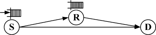
Figure 1: The system model.

The three-node relay communication link is depicted in Fig. 1. The source can select the relay or destination for data reception. In this model, there are buffers of infinite size at both the source and relay node. In this work, we assume full-duplex relay such that transmission and reception can be performed simultaneously. Note that full-duplex relaying can be achieved through some form of analog self-interference cancellation followed by digital self-interference cancellation in the baseband domain [31], [32].

The discrete-time input and output relationships in the $i$th symbol duration are given by

$$Y_{r}[i] =g_{sr}[i]X_{s}[i]+I[i]+n_{r}[i]$$ (1)

$$Y_{d}[i] =g_{sd}[i]X_{s}[i]+g_{rd}[i]X_{r}[i]+n_{d}[i]$$ (2)

where $X_{j}$ for $j\in\{s,r\}$ denote the input signal from the source S and the relay R, respectively. The inputs are subject to individual average energy constraints $\mathbb{E}\{|X_{j}|^{2}\}\leq\bar{P}_{j}/B,j\in\{s,r\}$ where $B$ is the bandwidth. $Y_{r},Y_{d}$ represent the received signal at the relay R and the destination D, respectively. We assume that the fading coefficients $g_{sd},g_{sr},g_{rd}$ are jointly stationary and ergodic discrete-time processes, and we denote the magnitude-square of the fading coefficients by $z_{sd}[i]=|g_{sd}[i]|^{2}$ , $z_{sr}[i]=|g_{sr}[i]|^{2}$, and $z_{rd}[i]=|g_{rd}[i]|^{2}$. Note that $I[i]$ denotes the self-interference incurred by the full-duplex operation at the relay, which may include linear and nonlinear components of the transmitted signal $X_{r}[i]$ of the relay [32]. In [31, Appendix A.1], the received signal’s SNR can be modeled as $\frac{\text{SNR}}{\gamma}$ with relative SNR loss $\gamma\geq 1$ due to self-interference. Hence, we normalize the channel gain of the link ${\textbf{S}}-{\textbf{R}}$ by $\gamma$ to take into account the self-interference, i.e., $\tilde{z}_{sr}=z_{sr}/\gamma$. Denote $\mathbf{z}=(z_{sd},\tilde{z}_{sr},z_{rd})$. Assuming that there are $B$ complex symbols per second, we can easily see that the symbol energy constraint of $\bar{P}_{j}/B$ implies that the channel input has a power constraint of $\bar{P}_{j}$. Above, in the channel input-output relationships, the noise component $n_{j}[i]$ is a zero-mean, circularly symmetric, complex Gaussian random variable with variance $\mathbb{E}\{|n_{j}[i]|^{2}\}=N_{0}$ for $j\in\{r,d\}$. The additive Gaussian noise samples $\{n_{j}[i]\}$ are assumed to form an independent and identically distributed (i.i.d.) sequence. We denote the signal-to-noise ratio at source as ${\text{\footnotesize{SNR}}}=\frac{\bar{P}_{s}}{N_{0}B}$, and at relay as ${\text{\footnotesize{SNR}}}_{r}=\frac{\bar{P}_{r}}{N_{0}B}$.

II-B Statistical Delay Constraits

With the above mentioned settings, we first need the following result from [33].

Theorem 1 ([33])

Suppose that the queue is stable and that both the arrival process $a[n],n=1,2,\dots$ and service process $c[n],n=1,2,\dots$ satisfy the Gärtner-Ellis limit, i.e., for all $\theta\geq 0$, there exists a differentiable logarithmic moment generating function (LMGF) $\Lambda_{A}(\theta)$ such that

$$\lim_{n\to\infty}\frac{\log\mathbb{E}\{e^{\theta\sum_{i=1}^{n}a[n]}\}}{n}=\Lambda_{A}(\theta),$$ (3)

and a differentiable LMGF $\Lambda_{C}(\theta)$ such that

$$\lim_{n\to\infty}\frac{\log\mathbb{E}\{e^{\theta\sum_{i=1}^{n}c[n]}\}}{n}=\Lambda_{C}(\theta).$$ (4)

If there exists a unique $\theta^{*}>0$ such that

$$\Lambda_{A}(\theta^{*})+\Lambda_{C}(-\theta^{*})=0,$$ (5)

then

$$\lim_{Q_{\text{{max}}}\to\infty}\frac{\log\Pr\{Q>Q_{\text{{max}}}\}}{Q_{\text{{max}}}}=-\theta^{*}.$$ (6)

where $Q$ is the stationary queue length. $\blacksquare$

This theorem tells us that the tail distribution of the stationary queue length decays exponentially. The proof of the theorem takes advantage of the large deviations principles (see e.g. [34] and [35]) to characterize the exponential decay rate of buffer overflow probability. In particular, for large $Q_{\text{{max}}}$, we have the approximation for the buffer violation probability: $\Pr\{Q>Q_{\text{{max}}}\}\approx e^{-\theta^{*}Q_{\text{{max}}}}$. Hence, while larger $\theta$ corresponds to more strict queueing constraints, smaller $\theta$ implies looser queueing constraints.

Assume that the first-in first-out (FIFO) queues are saturated, and hence they always attempt to transmit [14]. Then the queueing delay violation probability can be written equivalently as [17], [19]

$$\Pr\{D>D_{\text{{max}}}\}\doteq e^{-J(\theta)D_{\text{{max}}}}$$ (7)

where we defined $f(x)\doteq e^{cx}$ when $\lim_{x\to\infty}\frac{\log f(x)}{x}=c$, and

$$J(\theta)=\theta\delta=-\Lambda_{C}(-\theta)$$ (8)

is the statistical delay exponent associated with the queue, with $\Lambda_{C}(\theta)$ the LMGF of the service rate, and $\delta$ is decided by the arrival and departure processes jointly. Now, we can express the probability density function of random variable $D$ as

$$p_{D}(x)=\frac{\partial}{\partial x}\left(1-\Pr\{D>x\}\right)\doteq J(\theta)e^{-J(\theta)x}.$$ (9)

In this work, we seek to identify the maximum constant arrival rate to the source that can be supported by the relay system while satisfying the statistical delay constraints. Therefore, we need to guarantee that the data transmission of the flow with the largest end-to-end delay should satisfy the statistical delay constraints, i.e., information flow over two queues. Consider two concatenated queues with statistical queueing constraints specified by $\theta_{1}$ and $\theta_{2}$, for queue 1 and queue 2, respectively. Given the queueing constraints specified by $\theta_{1}$ and $\theta_{2}$ with (6) satisfied for each queue, we define

$$J_{1}(\theta_{1})=-\Lambda_{C,1}(-\theta_{1}),\,\,\text{and}\,\,J_{2}(\theta_{2})=-\Lambda_{C,2}(-\theta_{2}),$$ (10)

where $\Lambda_{C,1}(\theta_{1})$ and $\Lambda_{C,2}(\theta_{1})$ are the LMGF functions of the service rate of queue 1, 2, respectively. For data going through both queues, the end-to-end queueing delay violation probability can be characterized as

$$\Pr\{D_{1}+D_{2}>D_{\text{{max}}}\}\doteq 1-\int_{0}^{D_{\text{{max}}}}\int_{0}^{D_{\text{{max}}}-D_{1}}p_{D}(D_{1})p_{D}(D_{2})dD_{2}dD_{1}$$

$$=\left\{\begin{array}[]{ll}\frac{J_{1}(\theta_{1})e^{-J_{2}(\theta_{2})D_{\text{{max}}}}-J_{2}(\theta_{2})e^{-J_{1}(\theta_{1})D_{\text{{max}}}}}{J_{1}(\theta_{1})-J_{2}(\theta_{2})},&J_{1}(\theta_{1})\neq J_{2}(\theta_{2})\\ \left(1+J_{1}(\theta_{1})D_{\text{{max}}}\right)e^{-J_{1}(\theta_{1})D_{\text{{max}}}},&J_{1}(\theta_{1})=J_{2}(\theta_{2}).\end{array}\right.$$ (13)

Thereby, we need to guarantee that

$$\Pr\{D_{1}+D_{2}>D_{\text{{max}}}\}\leq\varepsilon.$$ (14)

In this way, we can guarantee that the data transmissions through the relay, i.e., information flow over two queues, satisfy the statistical delay constraints. Then, the delay constraints of the whole system can be satisfied. Note that $(\varepsilon,D_{\text{{max}}})$ characterizes the statistical delay constraints with maximum delay violation probability $\varepsilon$ and maximum delay $D_{\text{{max}}}$.

To facilitate the following analysis, we need the following tradeoff between $J_{1}(\theta_{1})$ and $J_{2}(\theta_{2})$.

Lemma 1 ([29])

Consider the following function

$$\vartheta(J_{1}(\theta_{1}),J_{2}(\theta_{2})) =\frac{J_{2}(\theta_{2})e^{-J_{1}(\theta_{1})D_{\text{{max}}}}-J_{1}(\theta_{1})e^{-J_{2}(\theta_{2})D_{\text{{max}}}}}{J_{2}(\theta_{2})-J_{1}(\theta_{1})}$$

$$=e^{-J_{0}D_{\text{{max}}}}=\varepsilon,\,\text{for}\,0\leq\varepsilon\leq 1,$$ (15)

where $J_{0}=-\frac{\log(\varepsilon)}{D_{\text{{max}}}}$ is defined as the statistical delay exponent associated with $(\varepsilon,D_{\text{{max}}})$. Denoting $J_{2}(\theta_{2})=\Phi(J_{1}(\theta_{1}))$ as a function of $J_{1}(\theta_{1})$, we have

1. $\Phi$ is continuous. For $J_{1}(\theta_{1})=J_{th}(\varepsilon)$, we have

   $$\Phi(J_{1}(\theta_{1}))=J_{th}(\varepsilon)$$ (16)

   where

   $$J_{th}(\varepsilon)=-\frac{1}{D_{\text{{max}}}}\left(1+\mathcal{W}_{-1}\left(-\frac{\varepsilon}{e}\right)\right)$$ (17)

   where $\mathcal{W}_{-1}(\cdot)$ is the Lambert W function, which is the inverse function of $y=xe^{x}$ in the range $(-\infty,-1]$.

2. $\Phi$ is strictly decreasing in $J_{1}(\theta_{1})$.

3. $\Phi$ is convex in $J_{1}(\theta_{1})$.

4. $J_{1}(\theta_{1})\in[J_{0},\infty)$, and $J_{2}(\theta_{2})=\Phi(J_{1}(\theta_{1}))\in[J_{0},\infty)$.

This lemma indicates that to have the end-to-end delay constraints satisfied, we must increase $J_{1}(\theta_{1})$ if $J_{2}(\theta_{2})$ is decreased; vice versa.

II-C Effective Capacity

Denote the queue at source S as queue 1, and the queue at relay R as queue 2. Denote $\Omega$ as the set of pairs $(\theta_{1},\theta_{2})$ such that (14) can be satisfied. Assume $\theta_{1}>0$ and $\theta_{2}>0$ at the source and the relay node with $(\theta_{1},\theta_{2})\in\Omega$. Assume that the constant arrival rate at the source is $R\geq 0$, and the channels operate at their capacities. Then, the effective capacity with statistical queueing constraints $(\theta_{1},\theta_{2})$ is defined as the maximum constant arrival rate such that both the queueing constraints can be satisfied. More specifically, to satisfy the queueing constraint at the source, we should have

$$\tilde{\theta}\geq\theta_{1}$$ (18)

where $\tilde{\theta}$ is the solution to

$$R=-\frac{\Lambda_{C,1}(-\tilde{\theta})}{\tilde{\theta}}$$ (19)

and $\Lambda_{C,1}(\theta)$ is the LGMF of the service rate for queue 1, i.e., queue at the source.

Also, in order to satisfy the queueing constraint of the relay node R, we must have

$$\hat{\theta}\geq\theta_{2}$$ (20)

where $\hat{\theta}$ is the solution to

$$\Lambda_{A,2}(\theta)+\Lambda_{C,2}(-\theta)=0.$$ (21)

where $\Lambda_{A,2}(\theta)$ is the LGMF of the arrival process to queue 2, $\Lambda_{C,2}(\theta)$ is the LGMF of the service process of queue 2, i.e., queue at the relay.

Note that we can derive the effective capacity $R_{E}(\theta_{1},\theta_{2})$ with $(\theta_{1},\theta_{2})$ following the method provided in [27, Theorem 2]. After these characterizations, effective capacity of the buffer-aided relay system under statistical delay constraints $(\varepsilon,D_{\text{{max}}})$ can be formulated as follows.

Definition 1

The effective capacity of the buffer-aided relay system with statistical delay constraints specified by $(\varepsilon,D_{\text{{max}}})$ is given by

$$R_{\varepsilon}(\varepsilon,D_{\text{{max}}})=\sup_{(\theta_{1},\theta_{2})\in\Omega}R_{E}(\theta_{1},\theta_{2}).$$ (22)

Hence, effective capacity is now the maximum constant arrival rate that can be supported by the relay system under statistical delay constraints.

III Effective Capacity with Selection Relaying Protocol in Block-Fading Channel

In the following, we first discuss the transmission strategy in detail to obtain the associated channel rate of the links. Then, assuming that $(\theta_{1},\theta_{2})$ are given, we obtain the effective bandwidth of the arrival processes of the queue at the relay given selection relaying policy. Next, we derive the effective capacity for arbitrary relay policy in a general form. Afterwards, we propose a relay policy taking into account the statistical delay constraints.

III-A Transmission Strategy and Channel Rate

We assume that perfect CSI of all links is available at S and R, while only the CSI of the links ${\textbf{S}}-{\textbf{D}}$ and ${\textbf{R}}-{\textbf{D}}$ is available at D. The transmission power levels at the source and relay are fixed and hence no power control is employed (i.e., nodes are subject to short-term power constraints). We further assume that the channel capacity for each link can be achieved, i.e., the service processes are equal to the instantaneous Shannon capacities of the links. We consider a block fading scenario in which the fading stays constant for a block of $T$ seconds and changes independently from one block to another.

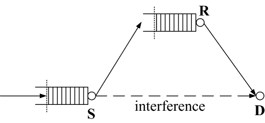
Figure 2: Select relay for sending information.

We consider selection relaying protocols, i.e., the source selects the relay for data reception when the channel condition at the relay is larger than certain threshold [2]. Denote $\mathcal{Z}$ as the region such that when $\mathbf{z}\in\mathcal{Z}$, the source S selects the relay R for data reception. Therefore, $\mathcal{Z}$ stands for the relay strategy employed in the system. The relay strategy is forwarded by the source to the destination through an one-bit acknowledge (ACK) signal such that the destination can perform successive decoding of the received signals when $\mathbf{z}\in\mathcal{Z}^{c}$.

When $\mathbf{z}\in\mathcal{Z}$, due to the buffer at the relay, the transmitted messages from the source and the relay node are different. So we cannot exploit spatial diversity as we can when there is no buffer at the relay. In this case, we have a two-hop channel while the transmitted signal of ${\textbf{S}}-{\textbf{R}}$ link forms interference to the ${\textbf{R}}-{\textbf{D}}$ link. See Fig. 2 for the illustration of the information flow. Then the instantaneous service rates for the queues at the source and relay node are given by

$$C_{sr} =TB\log_{2}(1+{\text{\footnotesize{SNR}}}\tilde{z}_{sr}),$$ (23)

$$C_{rd} =TB\log_{2}\left(1+\frac{{\text{\footnotesize{SNR}}}_{r}z_{rd}}{1+{\text{\footnotesize{SNR}}}z_{sd}}\right).$$ (24)

When $\mathbf{z}\in\mathcal{Z}^{c}$, S selects the destination D for data reception. In this case, we have a two-user multiple access channel. See Fig. 3 for the illustration of the information flow. Note that the destination can perform successive decoding of the received signal from the source and relay node. Define $\mathcal{Z}_{0}$ as the region depending on $z_{sd}$ and $z_{rd}$ such that when $\mathbf{z}\in\mathcal{Z}^{c}\cap\mathcal{Z}_{0}$, the destination D decodes the received signal in the order of $({\textbf{R}},{\textbf{S}})$, i.e., the sent signal from the source sees no interference, and the instantaneous rates are given by [36]

$$C_{sd} =TB\log_{2}(1+{\text{\footnotesize{SNR}}}z_{sd}),$$ (25)

$$C_{rd} =TB\log_{2}\left(1+\frac{{\text{\footnotesize{SNR}}}_{r}z_{rd}}{1+{\text{\footnotesize{SNR}}}z_{sd}}\right).$$ (26)

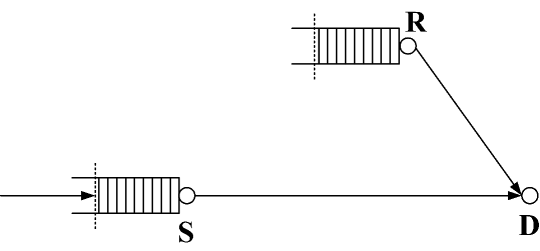
Figure 3: Select destination for sending information.

On the other hand, when $\mathbf{z}\in\mathcal{Z}^{c}\cap\mathcal{Z}_{0}^{c}$, the decoding order at D is $({\textbf{S}},{\textbf{R}})$, i.e., the sent signal from the relay sees no interference, and the instantaneous rates are given by

$$C_{sd} =TB\log_{2}\left(1+\frac{{\text{\footnotesize{SNR}}}z_{sd}}{1+{\text{\footnotesize{SNR}}}_{r}z_{rd}}\right),$$ (27)

$$C_{rd} =TB\log_{2}\left(1+{\text{\footnotesize{SNR}}}_{r}z_{rd}\right).$$ (28)

To summarize, we have the service rates of the queues at the source and relay node as

$$C_{s}=\left\{\begin{array}[]{ll}TB\log_{2}\left(1+{\text{\footnotesize{SNR}}}\tilde{z}_{sr}\right),&\mathbf{z}\in\mathcal{Z}\\ TB\log_{2}(1+{\text{\footnotesize{SNR}}}z_{sd}),&\mathbf{z}\in\mathcal{Z}^{c}\cap\mathcal{Z}_{0}\\ TB\log_{2}\left(1+\frac{{\text{\footnotesize{SNR}}}z_{sd}}{1+{\text{\footnotesize{SNR}}}_{r}z_{rd}}\right),&\mathbf{z}\in\mathcal{Z}^{c}\cap\mathcal{Z}_{0}^{c}\end{array}\right.$$ (32)

and

$$C_{r}=\left\{\begin{array}[]{ll}TB\log_{2}\left(1+\frac{{\text{\footnotesize{SNR}}}_{r}z_{rd}}{1+{\text{\footnotesize{SNR}}}z_{sd}}\right),&\mathbf{z}\in\mathcal{Z}\cup\{\mathcal{Z}^{c}\cap\mathcal{Z}_{0}\}\\ TB\log_{2}\left(1+{\text{\footnotesize{SNR}}}_{r}z_{rd}\right),&\mathbf{z}\in\mathcal{Z}^{c}\cap\mathcal{Z}_{0}^{c}\end{array}\right.$$ (35)

respectively. Above, the rates are in the units of bits per block or equivalently bits per $T$ seconds. These can be regarded as the service processes of the queues at the source and relay, respectively.

To ensure the stability of the queue at the relay, we need to enforce the following condition [33]

$$\mathbb{E}_{\mathbf{z}\in\mathcal{Z}}\{TB\log_{2}\left(1+{\text{\footnotesize{SNR}}}\tilde{z}_{sr}\right)\}<\mathbb{E}_{\mathbf{z}}\{C_{r}\}$$ (36)

where $\mathbb{E}_{\mathbf{z}\in\mathcal{Z}}\{\cdot\}$ denotes the expectation over the region $\mathcal{Z}$, i.e., $\int_{\mathbf{z}\in\mathcal{Z}}\left\{\cdot\right\}p_{\mathbf{z}}(\mathbf{z})d\mathbf{z}$ with $p_{\mathbf{z}}(\mathbf{z})$ the probability density function of $\mathbf{z}$. The above equation implies that the average arrival rate of the queue at the relay should be less than the average service rate. We assume that the above condition is satisfied for the relay policies in consideration, otherwise the effective capacity is deemed as zero.

III-B Effective Bandwidth of the S-R Link

Note that $\Lambda_{C,1}(\theta)$ and $\Lambda_{C,2}(\theta)$ can be easily derived with the relay policy $\mathcal{Z}$ after we obtain the service rate of queue 1 and 2 in (32) and (35), respectively. Then, from the discussions in Section II-C, we must obtain the effective bandwidth of the arrival processes of the queue at the relay to derive the effective capacity.

This can be achieved by borrowing the idea of intree-network [33]. Note that queue 1 is the predecessor of queue 2, or equivalently, queue 2 is the successor of queue 1. Now the three-node relay network can be viewed as an intree network. The routing depends on the relay protocol designed. Following the definitions in [33, Section 9.4], we define the routing variable

$$p_{1}[i]=\left\{\begin{array}[]{ll}1,&\mathbf{z}\in\mathcal{Z},\\ 0,&\mathbf{z}\in\mathcal{Z}^{c}.\end{array}\right.$$ (39)

That is, $p_{1}[i]=1$ if the departure from queue 1 at $i$th symbol is routed to the successor, i.e., queue 2, and $p_{1}[i]=0$ if the departure from queue 1 at $i$th symbol leaves the intree network, i.e., goes to the destination node. Now, we have the log-moment generating function for the routing process as

$$\Lambda_{p_{1}}(\theta,\mathcal{Z}) =\lim_{n\to\infty}\frac{\log\mathbb{E}\left\{e^{\theta\sum_{i=1}^{n}p_{1}[i]}\right\}}{n}.$$ (40)

Recalling the definitions in Section II-C, we have the following result.

Proposition 1

Given $(\theta_{1},\theta_{2})$ and the routing process specified by $\mathcal{Z}$, the LMGF of the departure process from the source to the relay, or equivalently the arrival process to the relay node, is given by

$$\Lambda_{A,2}(\theta)=\left\{\begin{array}[]{ll}R\Lambda_{p_{1}}(\theta,\mathcal{Z}),&0\leq\Lambda_{p_{1}}(\theta,\mathcal{Z})\leq\tilde{\theta},\\ R\tilde{\theta}+\Lambda_{C,1}\left(\Lambda_{p_{1}}(\theta,\mathcal{Z})-\tilde{\theta}\right),&\Lambda_{p_{1}}(\theta,\mathcal{Z})>\tilde{\theta}.\end{array}\right.$$ (43)

where $R$ is the constant arrival rate to queue 1, and $\tilde{\theta}$ is defined in (19).

Proof: Note that the only arrival to the relay node is from the source. Following the procedures described in [33, Section 9.4], we know that

$$\Lambda_{A,2}(\theta)=\Xi_{1}(\Lambda_{p_{1}}(\theta,\mathcal{Z}))$$ (44)

where $\Xi_{1}(\cdot)$ is the effective bandwidth of the departure process from queue 1. Since the arrival to the source is constant, we have

$$\Xi_{1}(\theta)=\left\{\begin{array}[]{ll}\theta R,&0\leq\theta\leq\tilde{\theta}\\ \tilde{\theta}R+\Lambda_{C,1}(\theta-\tilde{\theta}),&\theta>\tilde{\theta}.\end{array}\right.$$ (47)

Substituting the value of $\Lambda_{p_{1}}(\theta,\mathcal{Z})$ to the above equation yields the result directly. $\square$

III-C Effective Capacity

Under the block fading assumption, the logarithmic moment generating functions for the service processes of queues at the source S and the relay R as functions of $\theta$ are given by [16]

$$\Lambda_{C,1}(\theta) =\log\mathbb{E}\left\{e^{\theta C_{s}}\right\}\quad\text{and}\quad\Lambda_{C,2}(\theta)=\log\mathbb{E}\left\{e^{\theta C_{r}}\right\}$$ (48)

where $C_{s}$ and $C_{r}$ are given by (32) and (35), respectively. Now, due to the assumption that the fading changes independently from one block to another, we can, for instance, simplify the logarithmic moment generating function in (4) as $\Lambda_{C}=\lim_{n\to\infty}\frac{\log\mathbb{E}\{e^{\theta\sum_{i=1}^{n}c[i]}\}}{n}=\lim_{n\to\infty}\frac{\log\prod_{i=1}^{n}\mathbb{E}\{e^{\theta c[i]}\}}{n}=\lim_{n\to\infty}\frac{\sum_{i=1}^{n}\log\mathbb{E}\{e^{\theta c[i]}\}}{n}=\lim_{n\to\infty}\frac{n\log\mathbb{E}\{e^{\theta c[1]}\}}{n}=\log\mathbb{E}\{e^{\theta c[1]}\}$. If fading is correlated, such simplifications are in general not possible and analysis needs to be based on the limit forms of the asymptotic logarithmic moment generating functions. However, if the service rates can be regarded as Markov modulated processes, then it is shown in [33, Section 7.2] that $\lim_{n\to\infty}\frac{\log\mathbb{E}\{e^{\theta\sum_{i=1}^{n}c[i]}\}}{\theta n}=\frac{1}{\theta}\log\text{sp}(\phi(\theta)r)$ where $\text{sp}(A)$ denotes the spectral radius or equivalently the maximum of the absolute values of the eigenvalues of the matrix $A$, and $\phi(\theta)r$ is a matrix which depends on the transition probabilities of the Markov process. Similarly, we can derive the limit forms of the asymptotic logarithmic moment generating function of $p_{1}[i]$, $\lim_{n\to\infty}\frac{\log\mathbb{E}\{e^{\theta\sum_{i=1}^{n}p_{1}[i]}\}}{n}=\log\text{sp}(\varphi(\theta))$, if the routing process can be viewed as Markov modulated processes with $\varphi(\theta)$ representing the transition matrix of the associated Markov process. In such cases, an analysis similar to the one given in this paper can be pursued to identify the maximal effective capacity.

Combining (48) with (10) gives us $J_{1}(\theta_{1})$ and $J_{2}(\theta_{2})$ as follows

$$J_{1}(\theta_{1}) =-\log\Bigg{(}\mathbb{E}_{\mathbf{z}\in\mathcal{Z}}\left\{e^{-\theta_{1}TB\log_{2}(1+{\text{\footnotesize{SNR}}}\tilde{z}_{sr})}\right\}+\mathbb{E}_{\mathbf{z}\in\mathcal{Z}^{c}\cap\mathcal{Z}_{0}}\left\{e^{-\theta_{1}TB\log_{2}(1+{\text{\footnotesize{SNR}}}z_{sd})}\right\}$$

$$\hskip 56.9055pt+\mathbb{E}_{\mathbf{z}\in\mathcal{Z}^{c}\cap\mathcal{Z}_{0}^{c}}\left\{e^{-\theta_{1}TB\log_{2}\left(1+\frac{{\text{\footnotesize{SNR}}}z_{sd}}{1+{\text{\footnotesize{SNR}}}_{r}z_{rd}}\right)}\right\}\Bigg{)},$$ (49)

$$J_{2}(\theta_{2}) =-\log\Bigg{(}\mathbb{E}_{\mathbf{z}\in\mathcal{Z}\cup(\mathcal{Z}^{c}\cap\mathcal{Z}_{0})}\left\{e^{-\theta_{2}TB\log_{2}\left(1+\frac{{\text{\footnotesize{SNR}}}_{r}z_{rd}}{1+{\text{\footnotesize{SNR}}}z_{sd}}\right)}\right\}+\mathbb{E}_{\mathbf{z}\in\mathcal{Z}^{c}\cap\mathcal{Z}_{0}^{c}}\left\{e^{-\theta_{2}TB\log_{2}(1+{\text{\footnotesize{SNR}}}_{r}z_{rd})}\right\}\Bigg{)}.$$ (50)

Now, the LMGF for the routing process (40) can be written as

$$\Lambda_{p_{1}}(\theta,\mathcal{Z}) =\log\left(\Pr\{\mathbf{z}\in\mathcal{Z}^{c}\}+e^{\theta}\Pr\{\mathbf{z}\in\mathcal{Z}\}\right).$$ (51)

According to (43), the LMGF for the arrival process of the queue at the relay is

$$\Lambda_{A,2}(\theta)=\left\{\begin{array}[]{ll}R\Lambda_{p_{1}}(\theta,\mathcal{Z}),&0\leq\Lambda_{p_{1}}(\theta,\mathcal{Z})\leq\tilde{\theta},\\ R\tilde{\theta}+\log\mathbb{E}\left\{e^{\left(\Lambda_{p_{1}}(\theta,\mathcal{Z})-\tilde{\theta}\right)C_{s}}\right\},&\Lambda_{p_{1}}(\theta,\mathcal{Z})>\tilde{\theta}.\end{array}\right.$$ (54)

For the following analysis, we need to characterize the relationship between $\Lambda_{p_{1}}(\theta,\mathcal{Z})$ and $\theta$. We have the following result.

Lemma 2

Consider the function

$$\Lambda_{p_{1}}(\theta,\mathcal{Z})=\log\left(\Pr\{\mathbf{z}\in\mathcal{Z}^{c}\}+e^{\theta}\Pr\{\mathbf{z}\in\mathcal{Z}\}\right).$$ (55)

This function has the following properties:

1. $\Lambda_{p_{1}}(0,\mathcal{Z})=0$, and $\Lambda_{p_{1}}(\theta,\mathcal{Z})\leq\theta$.

2. $\Lambda_{p_{1}}(\theta,\mathcal{Z})$ is increasing in $\theta$.

3. $\Lambda_{p_{1}}(\theta,\mathcal{Z})$ is a convex function of $\theta$.

Proof:

1. This property can be readily seen by evaluating the function at $\theta=0$, and noting that $\Pr\{\mathbf{z}\in\mathcal{Z}\}\leq 1$.

2. The first derivative of $\Lambda_{p_{1}}$ with respect to $\theta$ can be evaluated as

   $$\dot{\Lambda}_{p_{1}}(\theta)=\frac{e^{\theta}\Pr\{\mathbf{z}\in\mathcal{Z}\}}{\Pr\{\mathbf{z}\in\mathcal{Z}^{c}\}+e^{\theta}\Pr\{\mathbf{z}\in\mathcal{Z}\}}>0.$$ (56)

   Hence, it is increasing in $\theta$.

3. This property follows immediately since $e^{\theta}$ is log-convex, and non-negative multiplication does not alter the convexity.

$\square$

Remark 1

Therefore, when $\theta=0$, we have $\Lambda_{p_{1}}(\theta,\mathcal{Z})=0$. As $\theta$ increases, $\Lambda_{p_{1}}(\theta,\mathcal{Z})$ increases. Also, $\Lambda_{p_{1}}(\theta,\mathcal{Z})$ increases at least linearly with $\theta$. Note that $\frac{\theta}{\Lambda_{p_{1}}(\theta,\mathcal{Z})}$ is decreasing in $\theta$, since the $\frac{\Lambda_{p_{1}}(\theta,\mathcal{Z})}{\theta}$ is increasing in $\theta$ [33]. Considering (56), we have

$$\lim_{\theta\to 0}\frac{\theta}{\Lambda_{p_{1}}(\theta,\mathcal{Z})}=\frac{1}{\dot{\Lambda}_{p_{1}}(0)}=\frac{1}{\Pr\{\mathbf{z}\in\mathcal{Z}\}}$$ (57)

where L’Hospital’s rule is used.

From Lemma 2, we can show that $\frac{J_{2}(\theta_{2})}{\Lambda_{p_{1}}(\theta_{2},\mathcal{Z})}$ is still a decreasing function of $\theta_{2}$ similar to [27, Lemma 1], which is fundamental to this article.

With the selection relaying strategy $\mathcal{Z}$, we can establish an upperbound on the arrival rates supported by the relay system with any specific $(\theta_{1},\theta_{2})$.

Proposition 2

The constant arrival rates, which can be supported by the buffering relay system with statistical queueing constraints specified by $(\theta_{1},\theta_{2})$ at the source and relay, respectively, are upperbounded by

$$R \leq\min\bigg{\{}-\frac{1}{\theta_{1}}\log\mathbb{E}\left\{e^{-\theta_{1}C_{s}}\right\},-\frac{1}{\Lambda_{p_{1}}(\theta_{2},\mathcal{Z})}\log\mathbb{E}\left\{e^{-\theta_{2}C_{r}}\right\}\bigg{\}}$$ (58)

$$=\min\left\{\frac{J_{1}(\theta_{1})}{\theta_{1}},\frac{J_{2}(\theta_{2})}{\Lambda_{p_{1}}(\theta_{2},\mathcal{Z})}\right\}$$ (59)

Proof: See Appendix -A. $\square$

Define

$$\Omega_{\varepsilon}=\{(\theta_{1},\theta_{2}):\text{ $J_{1}(\theta_{1})$ and $J_{2}(\theta_{2})$ are solutions to }\,(\ref{eq:J1J2relation})\}.$$

Similar to the discussions in [29] regarding two-hop channels, we can iterate over $(J_{1}(\theta_{1}),J_{2}(\theta_{2}))$ satisfying (1) and obtain the following result. Note that $z_{ij,\text{{max}}}$ and $z_{ij,\text{min}}$ represent the largest or smallest channel gain of link $i-j$, respectively.

Theorem 2

The effective capacity of the buffer-aided relay systems with selection relaying strategy $\mathcal{Z}$ subject to statistical delay constraints specified by $(\varepsilon,D_{\text{{max}}})$ is given by the following:

Case I: If $\theta_{1,th}=\Lambda_{p_{1}}(\theta_{2,th},\mathcal{Z})$,

$$R_{\varepsilon}(\varepsilon,D_{\text{{max}}})=\frac{J_{th}(\varepsilon)}{\theta_{1,th}},$$ (60)

where ($\theta_{1,th}$,$\theta_{2,th}$) is the unique solution pair to $J_{1}(\theta_{1})=J_{th}(\varepsilon)$, and $J_{2}(\theta_{2})=J_{th}(\varepsilon)$.

Case II: If $\theta_{1,th}>\Lambda_{p_{1}}(\theta_{2,th},\mathcal{Z})$,

$$R_{\varepsilon}(\varepsilon,D_{\text{{max}}})=\left\{\begin{array}[]{ll}\frac{J_{0}}{\theta_{1,0}},&TB\log_{2}\left(1+\frac{{\text{\footnotesize{SNR}}}_{r}z_{rd,\text{min}}}{1+{\text{\footnotesize{SNR}}}z_{sd,\text{{max}}}}\right),\\ &\geq\max\{TB\log_{2}(1+{\text{\footnotesize{SNR}}}\tilde{z}_{sr,\text{{max}}}),TB\log_{2}(1+{\text{\footnotesize{SNR}}}z_{sd,\text{{max}}})\}\\ \frac{J_{1}(\overset{\circ}{\theta}_{1})}{\overset{\circ}{\theta}_{1}},&\text{otherwise.}\end{array}\right.$$ (64)

where $\theta_{1,0}$ is the solution to $J_{1}(\theta_{1})=J_{0}$, and $\overset{\circ}{\theta}_{1}$ is the smallest value of $\theta_{1}$ with $(\theta_{1},\theta_{2})\in\Omega_{\varepsilon}$ satisfying

$$-\frac{1}{\theta_{1}}\log\mathbb{E}\left\{e^{-\theta_{1}C_{s}}\right\}=-\frac{1}{\theta_{1}}\Big{(}\log\mathbb{E}\left\{e^{-\theta_{2}C_{r}}\right\}$$

$$\hskip 42.67912pt+\log\mathbb{E}\left\{e^{(\Lambda_{p_{1}}(\theta_{2},\mathcal{Z})-\theta_{1})C_{s}}\right\}\Big{)}.$$ (65)

Moreover, if $\frac{dJ_{2}(\theta)}{d\theta}\big{|}_{\theta=\underline{\theta}_{1}}\leq\frac{dJ_{1}(\theta)}{d\theta}\big{|}_{\theta=\underline{\theta}_{1}}$, where $\underline{\theta}_{1}$ is given by $(\theta_{1},\theta_{2})\in\Omega_{\varepsilon}$ with

$$\theta_{1}=\Lambda_{p_{1}}(\theta_{2},\mathcal{Z}),$$ (66)

then the solution to (2) with $(\theta_{1},\theta_{2})\in\Omega_{\varepsilon}$ is unique.

Case III: If $\theta_{1,th}<\Lambda_{p_{1}}(\theta_{2,th},\mathcal{Z})$,

$$R_{\varepsilon}(\varepsilon,D_{\text{{max}}})=\left\{\begin{array}[]{ll}\frac{J_{0}}{\Lambda_{p_{1}}(\theta_{2,0},\mathcal{Z})},&\min\Big{\{}TB\log_{2}(1+{\text{\footnotesize{SNR}}}\tilde{z}_{sr,\text{min}}),\\ &TB\log_{2}\left(1+\frac{{\text{\footnotesize{SNR}}}z_{sd,\text{min}}}{1+{\text{\footnotesize{SNR}}}_{r}z_{rd,\text{{max}}}}\right)\Big{\}}\\ &\geq\frac{J_{0}}{\Lambda_{p_{1}}(\theta_{2,0},\mathcal{Z})}\\ \frac{J_{2}(\breve{\theta}_{2})}{\Lambda_{p_{1}}(\breve{\theta}_{2},\mathcal{Z})},&\text{otherwise.}\end{array}\right.$$ (71)

where $\theta_{2,0}$ is the solution to $J_{2}(\theta_{2})=J_{0}$, and ($\breve{\theta}_{1}$,$\breve{\theta}_{2}$) is the unique solution to

$$\frac{J_{1}(\theta_{1})}{\theta_{1}}=\frac{J_{2}(\theta_{2})}{\Lambda_{p_{1}}(\theta_{2},\mathcal{Z})}$$ (72)

with $(\theta_{1},\theta_{2})\in\Omega_{\varepsilon}$.

Proof: See Appendix -B. $\square$

Remark 2

The above theorem covers all the possibilities that symmetric or asymmetric delay constraints on the queues at the source and relay node can be optimal for achieving the maximum effective capacity of the relay system. Case I refers to the case that the maximum throughput can be achieved with symmetric delay constraints at the queues of the source and relay node. Case II represents the case when the statistical delay constraints at the relay can be more stringent, while Case III shows the scenario for more strict delay constraints at the source. Recalling [27, Theorem 2], we know that as $\varepsilon\to 1$, $\theta_{1}\to 0$ and $\theta_{2}\to 0$, and hence

$$\lim_{\varepsilon\to 1}R_{\varepsilon}(\varepsilon,D_{\text{{max}}}) =\min\left\{\lim_{\theta_{1}\to 0}\frac{J_{1}(\theta_{1})}{\theta_{1}},\lim_{\theta_{1}\to 0}\frac{J_{2}(\theta_{2})}{\Lambda_{p_{1}}(\theta_{2},\mathcal{Z})}\right\}$$ (73)

$$=\min\left\{\mathbb{E}\{C_{s}\},\frac{\mathbb{E}\{C_{r}\}}{\Pr\{\mathbf{z}\in\mathcal{Z}\}}\right\}.$$ (74)

III-D Selection Relaying Protocols

Considering the expression of the effective capacity and the associated conditions in Theorem 2, we note that finding the optimal relaying protocol in closed-form analytical expressions seems intractable for a general scenario. With this in mind, we consider a simplified case in which the relaying protocol is decided by a function of $\tilde{z}_{sr}$ and $z_{sd}$, and is denoted as $\tilde{z}_{sr}=g(z_{sd})$. The channel state region $\mathcal{Z}$ is given by

$$\mathcal{Z}=\{\mathbf{z}:\tilde{z}_{sr}>g(z_{sd})\}.$$ (75)

Also, assume that the decoding strategy at the destination is given by $z_{rd}=f(z_{sd})$, such that

$$\mathcal{Z}_{0}=\{\mathbf{z}:z_{rd}>f(z_{sd})\}.$$ (76)

III-D1 Max Channel Gain (MCG)

A typical relay policy with buffer-aided relay system is to select the link with stronger channel condition or received SNR [6]. Then, we have

$$g(z_{sd})=z_{sd}.$$ (77)

We know that $\mathcal{Z}=\{\mathbf{z}:\tilde{z}_{sr}>z_{sd}\}$. With this relaying scheme $\mathcal{Z}$, we can obtain the effective capacity according to Theorem 2.

III-D2 Max Delay Exponent (MDE)

In this part, we propose a relay policy that takes into account the statistical delay constraints as well. Assume that the optimal statistical queueing constraints $(\theta_{1},\theta_{2})\in\Omega_{\varepsilon}$ that maximize the effective capacity are given. With this parameter set $(\theta_{1},\theta_{2})$, we consider the relay strategy that maximizes the statistical delay exponent $J_{1}(\theta_{1})$ at the source, in which case the effective capacity can be potentially improved. Assume that the channel of the link ${\textbf{R}}-{\textbf{D}}$ is independent of the links ${\textbf{S}}-{\textbf{R}}$ and ${\textbf{S}}-{\textbf{D}}$. Combining (49), (75) and (76), we can express the statistical delay exponent $J_{1}(\theta_{1},g(z_{sd}))$ at the source as

$$J_{1}(\theta_{1},g(z_{sd})) =-\log\Bigg{(}\int_{0}^{\infty}\int_{g(z_{sd})}^{\infty}(1+{\text{\footnotesize{SNR}}}\tilde{z}_{sr})^{-\beta_{1}}p(z_{sd},\tilde{z}_{sr})d\tilde{z}_{sr}dz_{sd}$$

$$\hskip 14.22636pt+\int_{0}^{\infty}\int_{0}^{g(z_{sd})}\int_{f(z_{sd})}^{\infty}(1+{\text{\footnotesize{SNR}}}z_{sd})^{-\beta_{1}}p(z_{sd},\tilde{z}_{sr})p(z_{rd})dz_{rd}d\tilde{z}_{sr}dz_{sd}$$

$$\hskip 14.22636pt+\int_{0}^{\infty}\int_{0}^{g(z_{sd})}\int_{0}^{f(z_{sd})}\left(1+\frac{{\text{\footnotesize{SNR}}}z_{sd}}{1+{\text{\footnotesize{SNR}}}_{r}z_{rd}}\right)^{-\beta_{1}}p(z_{sd},\tilde{z}_{sr})p(z_{rd})dz_{rd}d\tilde{z}_{sr}dz_{sd}\Bigg{)}$$ (78)

Then, the associated relay strategy should be the solution to the following optimization problem

$$\max_{g}J_{1}(\theta_{1},g(z_{sd})).$$ (79)

We can obtain the relaying strategy specified as below.

Theorem 3

Given $(\theta_{1},\theta_{2})\in\Omega_{\varepsilon}$, the relay strategy as a function of $(z_{sd},\tilde{z}_{sr})$ that maximizes the statistical delay exponent at the source is given by

$$g(z_{sd},\theta_{1})=\frac{1}{{\text{\footnotesize{SNR}}}}\left(e^{-\frac{1}{\beta_{1}}\log\mathbb{E}_{z_{rd}}\left\{e^{-\theta_{1}C_{sd,\text{MAC}}}\right\}}-1\right)$$ (80)

where $\beta_{1}=\frac{\theta_{1}TB}{\log 2}$, and

$$C_{sd,\text{MAC}}=\left\{\begin{array}[]{ll}TB\log_{2}(1+{\text{\footnotesize{SNR}}}z_{sd}),&z_{rd}\geq f(z_{sd}),\\ TB\log_{2}\left(1+\frac{{\text{\footnotesize{SNR}}}z_{sd}}{1+{\text{\footnotesize{SNR}}}_{r}z_{rd}}\right),&z_{rd}<f(z_{sd}).\end{array}\right.$$ (83)

Proof: Define $\hat{g}(z_{sd})=g(z_{sd},\theta_{1})+s\eta(z_{sd})$, where $g(z_{sd},\theta_{1})$ is the optimal function, $s$ is any constant, and $\eta(z_{sd})$ represents arbitrary perturbation. Now, a necessary condition that needs to be satisfied for the solution to (79) is [37]

$$\frac{d}{ds}\left(J_{1}(\theta_{1},\hat{g}(z_{sd}))\right)\bigg{|}_{s=0}=0.$$ (84)

By noting that $\frac{d\hat{g}(z_{sd})}{ds}=\eta(z_{sd})$, and from (III-D2) and (84), we can obtain

$$\int_{0}^{\infty}\bigg{(}-\left(1+{\text{\footnotesize{SNR}}}g(z_{sd},\theta_{1})\right)^{-\beta_{1}}+\int_{f(z_{sd})}^{\infty}(1+{\text{\footnotesize{SNR}}}z_{sd})^{-\beta_{1}}p(z_{rd})dz_{rd}$$

$$+\int_{0}^{f(z_{sd})}\left(1+\frac{{\text{\footnotesize{SNR}}}z_{sd}}{1+{\text{\footnotesize{SNR}}}_{r}z_{rd}}\right)^{-\beta_{1}}p(z_{rd})dz_{rd}\bigg{)}p(z_{sd},g(z_{sd},\theta_{1}))\eta(z_{sd})dz_{sd}=0$$ (85)

Since the above equation holds for any $\eta(z_{sd})$, it follows that

$$-\left(1+{\text{\footnotesize{SNR}}}g(z_{sd},\theta_{1})\right)^{-\beta_{1}}+\int_{f(z_{sd})}^{\infty}(1+{\text{\footnotesize{SNR}}}z_{sd})^{-\beta_{1}}p(z_{rd})dz_{rd}$$

$$+\int_{0}^{f(z_{sd})}\left(1+\frac{{\text{\footnotesize{SNR}}}z_{sd}}{1+{\text{\footnotesize{SNR}}}_{r}z_{rd}}\right)^{-\beta_{1}}p(z_{rd})dz_{rd}=0$$ (86)

which after rearranging and defining $C_{sd,\text{MAC}}$ shown in (83) yields (80). $\square$

Theorem 4

With the optimal $g(z_{sd},\theta_{1})$, we can show the following:

1. $J_{1}(\theta_{1},g(z_{sd},\theta_{1}))$ is increasing in $\theta_{1}$.

2. $\frac{J_{1}(\theta_{1},g(z_{sd},\theta_{1}))}{\theta_{1}}$ is decreasing in $\theta_{1}$.

Proof: See Appendix -C. $\square$

With the above properties, we know that given $J_{1}$, there is a unique $\theta_{1}$ with $g(z_{sd},\theta_{1})$ achieving $J_{1}(\theta_{1},g(z_{sd},\theta_{1}))=J_{1}$, and as $J_{1}$ increases, $\theta_{1}$ increases, and $\frac{J_{1}(\theta_{1},g(z_{sd},\theta_{1}))}{\theta_{1}}$ decreases. Therefore, as we iterate over $(\theta_{1},\theta_{2})\in\Omega_{\varepsilon}$, we know that the achievable rate of the relay system decreases as $\theta_{1}$, or equivalently $J_{1}(\theta_{1})$, increases. Then, we can still apply the method in Theorem 2 to obtain the maximum effective capacity associated with the proposed relay policy. Instead of fixed relaying policy $\mathcal{Z}$, we now have different $\mathcal{Z}=\{\mathbf{z}:\tilde{z}_{sr}>g(z_{sd},\theta_{1})\}$ for different $(J_{1}(\theta_{1}),J_{2}(\theta_{2}))$.

Remark 3

As $\varepsilon\to 1$, i.e., $\theta_{1}\to 0$ and $\theta_{2}\to 0$, we have

$$g(z_{sd},0)=\frac{1}{{\text{\footnotesize{SNR}}}}\left(e^{\mathbb{E}_{z_{rd}}\{C_{sd,\text{MAC}}\}}-1\right).$$ (87)

This is equivalent to selecting the relay when the instantaneous channel rate of ${\textbf{S}}-{\textbf{R}}$ is larger than the average channel rate of ${\textbf{S}}-{\textbf{D}}$ given $z_{sd}$. Note that $g(z_{sd},0)<z_{sd}$, and hence the source may select the relay for transmission even when the link ${\textbf{S}}-{\textbf{D}}$ is better due to the potential interference from the relay. In this case, according to Theorem 2, we have the achievable throughput given by

$$\min\left\{\mathbb{E}\{C_{s}\},\frac{\mathbb{E}\{C_{r}\}}{\Pr\{\tilde{z}_{sr}>g(z_{sd},0)\}}\right\}$$ (88)

where the first term is the average service rate of the queue at the source, while the second term is the maximum supported rate considering the buffer at the relay.

Remark 4

If $f(z_{sd})=0$, i.e., the destination always decodes the signal from S last, we know that $g(z_{sd},\theta_{1})=z_{sd}$, i.e., the proposed relay policy reduces to the max channel gain selection.

III-D3 No-Buffer Relay

For comparison, we also consider the performance of the relay system without buffer at the relay. We assume buffer at the source node only. Information-theoretical analysis have shown that the maximum rate for the three-node relay network with DF is given by [2]

$$C=\frac{TB}{2}\min\{\log_{2}(1+2{\text{\footnotesize{SNR}}}z_{sr}),\log_{2}(1+2{\text{\footnotesize{SNR}}}z_{sd}+2{\text{\footnotesize{SNR}}}z_{rd})\}.$$ (89)

The effective capacity associated with arbitrary queueing constraints $\theta$ is

$$R(\theta)=-\frac{1}{\theta}\log\mathbb{E}\{e^{-\theta C}\}.$$ (90)

Then, to guarantee the statistical delay constraints $(\varepsilon,D_{\text{{max}}})$, we should have from (7)

$$\theta R(\theta)\geq-\frac{\log\varepsilon}{D_{\text{{max}}}}.$$ (91)

Since $R(\theta)$ is decreasing in $\theta$, there must be one smallest $\theta_{\text{min}}$ such that the above inequality holds with equality. The maximum achievable throughput is then given by $R(\theta_{\text{min}})$.

IV Numerical Results

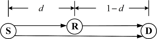
Figure 4: The relay model.

We consider the relay model depicted in Fig. 4. The source, relay, and destination nodes are located on a straight line. The distance between the source and the destination is normalized to 1. Let the distance between the source and the relay node be $d\in(0,1)$. Then, the distance between the relay and the destination is $1-d$. We assume the fading distributions for ${\textbf{S}}-{\textbf{D}}$, ${\textbf{S}}-{\textbf{R}}$ and ${\textbf{R}}-{\textbf{D}}$ links follow independent Rayleigh fading with means $\mathbb{E}\{z_{sd}\}=1$, $\mathbb{E}\{z_{sr}\}=1/d^{\alpha}$ and $\mathbb{E}\{z_{rd}\}=1/(1-d)^{\alpha}$, respectively, where we assume that the path loss $\alpha=4$. We assume ${\text{\footnotesize{SNR}}}=0$ dB, $T=1$ ms, $B=180$ kHz, and $f(z_{sd})=z_{sd}$ in the following numerical results. It has been demonstrated that almost ideal full-duplex relaying can be achieved (1.87$\times$ gain in median throughput compared with 2$\times$ of the ideal case (see [32, Section 5.3])). Therefore, without loss of generality, we assume ideal full-duplex relay with $\gamma=1$, i.e., $\tilde{z}_{sr}=z_{sr}$. Note that larger $\gamma$ implies stronger residual self-interference at the relay, which decreases the received SNR at the relay, and hence the achievable throughput of the system.

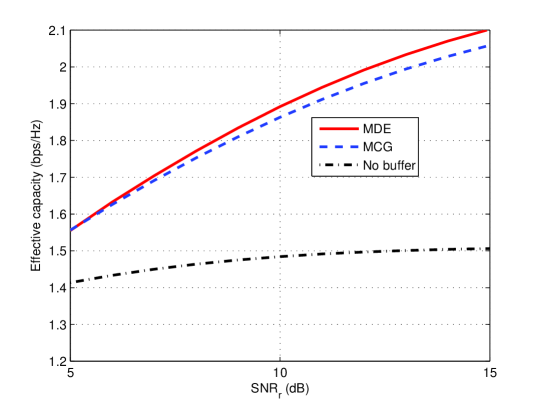
Figure 5: Effective capacity as a function of ${\text{\footnotesize{SNR}}}_{r}$. $\varepsilon=0.05$.

In Fig. 5, we plot the effective capacities for the different relay policies as a function of ${\text{\footnotesize{SNR}}}_{r}$ of the relay node. We assume $d=0.5$, $\varepsilon=0.05$. We can see from the figure that buffering relay can still help improve the system throughput under statistical delay constraints. In addition, the proposed relay policy can achieve better performance than the policy that selects relay with stronger channel condition. As ${\text{\footnotesize{SNR}}}_{r}$ increases, the achievable throughput without buffer at relay approaches some finite value, since the service rate of the queue at the source is limited by $\frac{TB}{2}\log_{2}(1+2{\text{\footnotesize{SNR}}}z_{sr})$.

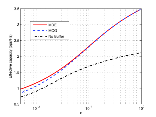
Figure 6: Effective capacity as a function of $\varepsilon$. ${\text{\footnotesize{SNR}}}_{r}=10$ dB. $d=0.5$.

In Fig. 6, we plot the effective capacity as $\varepsilon$ varies for ${\text{\footnotesize{SNR}}}_{r}=10$ dB. We assume $d=0.5$. As $\varepsilon\to 1$, we know that the effective capacity approaches the value given by (88). It is interesting that the proposed relay policy can achieve better performance than the best relay selection policy, and the improvement can be enlarged at smaller $\varepsilon$, i.e., more stringent delay constraints. We can also find that buffering relay helps improve the throughput for a wide range of statistical delay constraints.

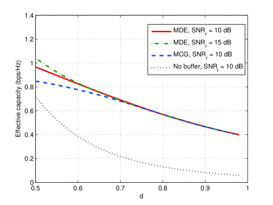
Figure 7: Effective capacity as $d$ varies. $\varepsilon=0.005$.

In Fig. 7, we plot the effective capacity as $d$ varies. We assume $\varepsilon=0.005$. We can find that as $d$ increases, i.e., the channel condition between the link ${\textbf{S}}-{\textbf{R}}$ is worse, the effective capacity decreases. The improvement of the proposed relay policy over the best relay selection policy can be larger at smaller $d$, i.e., stronger ${\textbf{S}}-{\textbf{R}}$ link. Also, it is interesting that as $d$ increases, the performance improvement of buffering relay becomes larger. This is mostly because the ${\textbf{S}}-{\textbf{R}}$ now limits the achievable rate of the relay system considering (89). On the other hand, due to the selection relaying protocol that takes advantage of the link ${\textbf{S}}-{\textbf{R}}$ when its channel is more favorable, significant performance gain can be obtained. Note also that the increase of SNR at the relay helps little as $d$ increases, since the buffer at the source is now the bottle-neck of the system. More specifically, as $d$ approaches to 1, the channel between ${\textbf{R}}-{\textbf{D}}$ grows unbounded, i.e., $TB\log_{2}\left(1+\frac{{\text{\footnotesize{SNR}}}_{r}z_{rd,\text{min}}}{1+{\text{\footnotesize{SNR}}}z_{sd,\text{{max}}}}\right)\geq\max\{TB\log_{2}(1+{\text{\footnotesize{SNR}}}\tilde{z}_{sr,\text{{max}}}),TB\log_{2}(1+{\text{\footnotesize{SNR}}}z_{sd,\text{{max}}})\}$. Then, the effective capacity is given by (64), where the impact of ${\text{\footnotesize{SNR}}}_{r}$ on $\theta_{1,0}$ is very small.

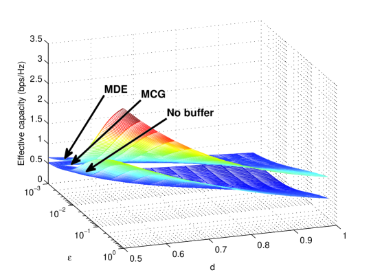
Figure 8: Effective capacity as $d$ and $\varepsilon$ vary. ${\text{\footnotesize{SNR}}}_{r}=10$ dB.

In Fig. 8, we plot the effective capacity as $d$ and $\varepsilon$ vary. We assume ${\text{\footnotesize{SNR}}}_{r}=10$ dB. We can see from the figure that the improvement provided by the proposed relay policy over the best relay selection policy is more obvious at relatively smaller $\varepsilon$, i.e., more stringent delay constraints. As can be seen from the figure, for all cases considered, the performance of buffering relay systems is better, albeit the improvement vanishes as delay constraints become more stringent.

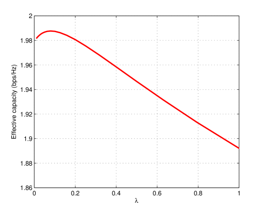
Figure 9: Effective capacity vs. $\lambda$. ${\text{\footnotesize{SNR}}}_{r}=10$ dB. $d=0.5$. $\varepsilon=0.05$.

Finally, we are interested in the impact of decoding strategy $\mathcal{Z}_{0}$ in (76) employed at the destination. Assume $f(z_{sd})=\lambda z_{sd}$. We plot the effective capacity of the proposed strategy as $\lambda$ varies for ${\text{\footnotesize{SNR}}}_{r}=10$ dB in Fig. 9. It is interesting that there is an optimal $\lambda$ that maximizes the effective capacity, after which value the effective capacity starts to decrease as $\lambda$ increases. Note that as $\lambda$ increases, $\mathcal{Z}_{0}$ shrinks. Now, the service rate of ${\textbf{S}}-{\textbf{D}}$ decreases, while the service rate of ${\textbf{R}}-{\textbf{D}}$ increases according to (32) and (35). Hence, as $\mathcal{Z}_{0}$ shrinks, while the improvement in the link ${\textbf{R}}-{\textbf{D}}$ helps increase the throughput, the deterioration in the link ${\textbf{S}}-{\textbf{D}}$ decreases the throughput. There should be a tradeoff such that the overall throughput can be optimized. Finding the optimal decoding strategy is beyond the topic of this work, and is left for future extension.

V Conclusion

In this paper, we have analyzed the maximum arrival rates that can be supported by a full-duplex buffer-aided relaying system under statistical delay constraints. We have assumed that both the source and the relay have perfect CSI of the all links, while the destination is not aware of the CSI of source-relay link. We have assumed that the source selects the destination or the relay for data reception based on the selection relaying strategy, which is informed to the destination by the source through an ACK signal such that the destination can perform simultaneous decoding of the received signal. Given arbitrary selection relay policy, we have expressed the effective bandwidth of the departure process from the queue at the source. We have obtained the maximum effective capacity under statistical end-to-end delay constraints. In the subsequent analysis, we have proposed a relay policy that takes into account the statistical delay constraints as well. Through numerical results, we have shown that the delay constraint based relay scheme can achieve better performance than the max channel gain selection policy. Also, we have found that buffering relay can still help improve the throughput in the presence of statistical delay constraints and direct transmission link.

-A Proof of Proposition 2

For given $\theta_{1}$ and $\theta_{2}$, we can see from (18) that

$$R=-\frac{1}{\tilde{\theta}}\log\mathbb{E}\left\{e^{-\tilde{\theta}C_{s}}\right\}\leq-\frac{1}{\theta_{1}}\log\mathbb{E}\left\{e^{-\theta_{1}C_{s}}\right\}.$$ (92)

Note that the above inequality follows immediately from the assumption that $\tilde{\theta}\geq\theta_{1}$ and $-\frac{\Lambda_{C,1}(-\tilde{\theta})}{\tilde{\theta}}=-\frac{1}{\tilde{\theta}}\log\mathbb{E}\left\{e^{-\tilde{\theta}C_{s}}\right\}$ is a decreasing function of $\tilde{\theta}$.

Proving another upperbound is a little tricky. Consider the idealistic scenario in which the ${\textbf{S}}-{\textbf{D}}$ and ${\textbf{S}}-{\textbf{R}}$ links are deterministic (i.e., there is no fading) and additionally can support any constant arrival rate $R>-\frac{1}{\Lambda_{p_{1}}(\theta_{2})}\log\mathbb{E}\left\{e^{-\theta_{2}C_{r}}\right\}$. Now, the arriving data to the source can immediately be sent without waiting and consequently there is no need for buffering at the source. Hence, any source queueing constraints can be satisfied. Moreover, assume the source selects relay for transmission with probability $\Pr\{\mathbf{z}\in\mathcal{Z}\}$. With this routing decision, we can see that $\Lambda_{p_{1}}(\theta_{1},\mathcal{Z})$ in (40) is unchanged. If the service rate matches the constant arrival rate, i.e., $C_{s}=R$, the equation in (19) holds for any $\tilde{\theta}$. That is

$$R=-\frac{\Lambda_{C,1}(-\tilde{\theta})}{\tilde{\theta}}=-\frac{1}{\tilde{\theta}}\log\mathbb{E}\left\{e^{-\tilde{\theta}R}\right\}=-\frac{1}{\tilde{\theta}}(-\tilde{\theta}R)=R$$ (93)

where the instantaneous service rate is assumed to be equal to the constant arrival rate $R$. Since no buffering is now required at the source, we can freely impose the most strict QoS constraints and assume $\tilde{\theta}$ to be unbounded as well. Then, with the relay strategy and Lemma 2, we have $\Lambda_{p_{1}}(\hat{\theta},\mathcal{Z})\leq\hat{\theta}\leq\tilde{\theta}$ for any $\hat{\theta}$. With this, we see from (21) that

$$R=-\frac{1}{\Lambda_{p_{1}}(\hat{\theta},\mathcal{Z})}\log\mathbb{E}\left\{e^{-\hat{\theta}C_{r}}\right\}\leq-\frac{1}{\Lambda_{p_{1}}(\theta_{2},\mathcal{Z})}\log\mathbb{E}\left\{e^{-\theta_{2}C_{r}}\right\}$$ (94)

where the inequality follows since $-\frac{1}{\Lambda_{p_{1}}(\theta,\mathcal{Z})}\log\mathbb{E}\left\{e^{-\theta C_{r}}\right\}$ is decreasing in $\theta$ and $\hat{\theta}\geq\theta_{2}$. Combining the bounds in (92) and (94), we can equivalently write

$$R\leq\min\left\{-\frac{1}{\theta_{1}}\log\mathbb{E}\left\{e^{-\theta_{1}C_{s}}\right\},-\frac{1}{\Lambda_{p_{1}}(\theta_{2},\mathcal{Z})}\log\mathbb{E}\left\{e^{-\theta_{2}C_{r}}\right\}\right\}.$$ (95)

$\square$

-B Proof of Theorem 2

The idea of this proof follows that in [29, Appendix C], except that the effective bandwidth of the arrival process to the queue at the relay is now given by (54), and the upperbound on the effective capacity is given by (58) instead. We here give the sketch of the proof.

We seek to find the optimal $J_{1}(\theta_{1})$ and $J_{2}(\theta_{2})$ on the lower boundary curve specified by Lemma 1. We first start from the point $J_{1}(\theta_{1})=J_{2}(\theta_{2})=J_{th}(\varepsilon)$. From (49) and (50), we can obtain the associated $\theta_{1,th}$ and $\theta_{2,th}$, which are solutions to

$$J_{1}(\theta_{1,th})=J_{th}(\varepsilon),\,\text{and}\,J_{2}(\theta_{2,th})=J_{th}(\varepsilon).$$ (96)

Compute $\Lambda_{p_{1}}(\theta_{2,th},\mathcal{Z})$ from (55). Depending on the relationship between $\theta_{1,th}$ and $\Lambda_{p_{1}}(\theta_{2,th},\mathcal{Z})$, we have three different cases.

Case I: Assume $\theta_{1,th}=\Lambda_{p_{1}}(\theta_{2,th})$. We can show that the effective capacity of the relay system is given by

$$R_{\varepsilon}(\varepsilon,D_{\text{{max}}})=\sup_{(\theta_{1},\theta_{2})\in\Omega}R_{E}(\theta_{1},\theta_{2})=R_{E}(\theta_{1,th},\theta_{2,th})=\frac{J_{th}(\varepsilon)}{\theta_{1,th}}=\frac{J_{th}(\varepsilon)}{\Lambda_{p_{1}}(\theta_{2,th},\mathcal{Z})},$$ (97)

considering Proposition 2.

Case II: Assume $\theta_{1,th}>\Lambda_{p_{1}}(\theta_{2,th},\mathcal{Z})$. In this case, we can relieve the queueing constraints at the source, i.e., decrease $\theta_{1}$, or $J_{1}(\theta_{1})$ equivalently. Correspondingly, according to Lemma 1, $J_{2}(\theta_{2})$, and hence $\theta_{2}$, should increase. We can show that the queue at the relay will not affect the performance as long as $\theta_{1}$ and $\Lambda_{p_{1}}(\theta_{2},\mathcal{Z})$ satisfies the following inequality given by

$$-\frac{1}{\theta_{1}}\log\mathbb{E}\left\{e^{-\theta_{1}C_{s}}\right\} \leq-\frac{1}{\theta_{1}}\left(\log\mathbb{E}\left\{e^{-\theta_{2}C_{r}}\right\}+\log\mathbb{E}\left\{e^{(\Lambda_{p_{1}}(\theta_{2},\mathcal{Z})-\theta_{1})C_{s}}\right\}\right)$$

$$=\frac{\theta_{2}}{\theta_{1}}\left(-\frac{1}{\theta_{2}}\log\mathbb{E}\left\{e^{-\theta_{2}C_{r}}\right\}-\frac{1}{\theta_{2}}\log\mathbb{E}\left\{e^{(\Lambda_{p_{1}}(\theta_{2},\mathcal{Z})-\theta_{1})C_{s}}\right\}\right).$$ (98)

Note that in the limit as $J_{2}(\theta_{2})\to\infty$, or $\theta_{2}\to\infty$, we have

$$\lim_{\theta_{2}\to\infty}-\frac{1}{\theta_{2}}\log\mathbb{E}\left\{e^{-\theta_{2}C_{r}}\right\}=\min C_{r}=TB\log_{2}\left(1+\frac{{\text{\footnotesize{SNR}}}_{r}z_{rd,\text{min}}}{1+{\text{\footnotesize{SNR}}}z_{sd,\text{{max}}}}\right)$$ (99)

the minimum service rate of the queue at relay. Also,

$$\lim_{\theta_{2}\to\infty}\frac{1}{\theta_{2}}\log\mathbb{E}\left\{e^{(\Lambda_{p_{1}}(\theta_{2},\mathcal{Z})-\theta_{1})C_{s}}\right\}=\max C_{s}=\max\{TB\log_{2}(1+{\text{\footnotesize{SNR}}}\tilde{z}_{sr,\text{{max}}}),TB\log_{2}(1+{\text{\footnotesize{SNR}}}z_{sd,\text{{max}}})\}$$ (100)

the maximum service rate of the queue at source. If $TB\log_{2}\left(1+\frac{{\text{\footnotesize{SNR}}}_{r}z_{rd,\text{min}}}{1+{\text{\footnotesize{SNR}}}z_{sd,\text{{max}}}}\right)>\max\{TB\log_{2}(1+{\text{\footnotesize{SNR}}}\tilde{z}_{sr,\text{{max}}}),TB\log_{2}(1+{\text{\footnotesize{SNR}}}z_{sd,\text{{max}}})\}$, we know that there is no congestion at the relay node at all. Then, the queue at the source is the bottle-neck of the relay system, and the effective capacity is

$$R_{\varepsilon}(\varepsilon,D_{\text{{max}}})=\frac{J_{0}}{\theta_{1,0}}$$ (101)

where $J_{0}$ is defined in (1), and $\theta_{1,0}$ is the solution to $J_{1}(\theta_{1})=J_{0}$. Otherwise, we have $(\overset{\circ}{\theta}_{1},\overset{\circ}{\theta}_{2})\in\Omega_{\varepsilon}$ such that $\overset{\circ}{\theta}_{1}$ is the smallest value of $\theta_{1}$ while (-B) can be satisfied with equality at $(\theta_{1},\theta_{2})$. Now, we can show that the effective capacity is given by

$$R_{\varepsilon}(\varepsilon,D_{\text{{max}}})=\sup_{(\theta_{1},\theta_{2})\in\Omega}R_{E}(\theta_{1},\theta_{2})=R_{E}(\overset{\circ}{\theta}_{1},\overset{\circ}{\theta}_{2})=\frac{J_{1}(\overset{\circ}{\theta}_{1})}{\overset{\circ}{\theta}_{1}}.$$ (102)

Also, similar to [29, Lemma 4], we can show the condition for the uniqueness of $(\overset{\circ}{\theta}_{1},\overset{\circ}{\theta}_{2})$.

Case III: Assume $\theta_{1,th}<\Lambda_{p_{1}}(\theta_{2,th},\mathcal{Z})$. In this case, we should relieve the queueing constraints at the relay instead, i.e., decrease $\theta_{2}$, or $J_{2}(\theta_{2})$ equivalently. So we should have larger $\theta_{1}$, or $J_{1}(\theta_{1})$, from Lemma 1. Then, we know that the effective capacity with $\theta_{1}>\Lambda_{p_{1}}(\theta_{2},\mathcal{Z})$ is given by

$$\min\left\{-\frac{1}{\theta_{1}}\log\mathbb{E}\left\{e^{-\theta_{1}C_{s}}\right\},-\frac{1}{\Lambda_{p_{1}}(\theta_{2},\mathcal{Z})}\log\mathbb{E}\left\{e^{-\theta_{2}C_{r}}\right\}\right\}.$$ (103)

Note that in the limit as $J_{1}(\theta_{1})\to\infty$, or $\theta_{1}\to\infty$, we have

$$\lim_{\theta_{1}\to\infty}-\frac{1}{\theta_{1}}\log\mathbb{E}\left\{e^{-\theta_{1}C_{s}}\right\} =\min C_{s}$$

$$=\min\left\{TB\log_{2}(1+{\text{\footnotesize{SNR}}}\tilde{z}_{sr,\text{min}}),TB\log_{2}\left(1+\frac{{\text{\footnotesize{SNR}}}z_{sd,\text{min}}}{1+{\text{\footnotesize{SNR}}}_{r}z_{rd,\text{{max}}}}\right)\right\}$$ (104)

the minimum service rate of the queue at the source. Also, as $J_{1}(\theta_{1})\to\infty$, we have $J_{2}(\theta_{2})\to J_{0}$ from Lemma 1, and $\theta_{2}\to\theta_{2,0}$, which is the solution to $J_{2}(\theta_{2})=J_{0}$. Now

$$\lim_{\theta_{1}\to\infty}-\frac{1}{\Lambda_{p_{1}}(\theta_{2},\mathcal{Z})}\log\mathbb{E}\left\{e^{-\theta_{2}C_{r}}\right\}=\frac{J_{0}}{\Lambda_{p_{1}}(\theta_{2,0},\mathcal{Z})}.$$ (105)

If $\min\left\{TB\log_{2}(1+{\text{\footnotesize{SNR}}}\tilde{z}_{sr,\text{min}}),TB\log_{2}\left(1+\frac{{\text{\footnotesize{SNR}}}z_{sd,\text{min}}}{1+{\text{\footnotesize{SNR}}}_{r}z_{rd,\text{{max}}}}\right)\right\}>\frac{J_{0}}{\Lambda_{p_{1}}(\theta_{2,0},\mathcal{Z})}$, we know that the queue at the relay is the bottle-neck of the relay system, and the effective capacity is

$$R_{\varepsilon}(\varepsilon,D_{\text{{max}}})=\frac{J_{0}}{\Lambda_{p_{1}}(\theta_{2,0},\mathcal{Z})}.$$ (106)

Otherwise, we can find a unique pair of $(\breve{\theta}_{1},\breve{\theta}_{2})\in\Omega_{\varepsilon}$ such that $\frac{J_{1}(\breve{\theta}_{1})}{\breve{\theta}_{1}}=\frac{J_{2}(\breve{\theta}_{2})}{\Lambda_{p_{1}}(\breve{\theta}_{2},\mathcal{Z})}$. We can show that the effective capacity is now given by

$$R_{\varepsilon}(\varepsilon,D_{\text{{max}}})=\sup_{(\theta_{1},\theta_{2})\in\Omega}R_{E}(\theta_{1},\theta_{2})=R_{E}(\breve{\theta}_{1},\breve{\theta}_{2})=\frac{J_{2}(\breve{\theta}_{2})}{\Lambda_{p_{1}}(\breve{\theta}_{2},\mathcal{Z})}.$$ (107)

The details of the derivation for the above claims are similar to the proof in [29, Appendix C], and are omitted here. Interested readers are encouraged to find more details in [29, Appendix C]. $\square$

-C Proof of Theorem 4

1. This can be easily verified since for $\theta_{1}^{\prime}>\theta_{1}$, we have

   $$J_{1}(\theta_{1}^{\prime},g(z_{sd},\theta_{1}^{\prime}))>J_{1}(\theta_{1}^{\prime},g(z_{sd},\theta_{1}))>J_{1}(\theta_{1},g(z_{sd},\theta_{1}))$$ (108)

   where the first inequality holds due to the definition of $g(z_{sd},\theta_{1}^{\prime})$, and the second inequality holds since given relay policy $g$, $J_{1}(\theta_{1},g)$ is an increasing function of $\theta_{1}$.

2. Taking the derivative of $J_{1}(\theta_{1},g(z_{sd},\theta_{1}))$ with respect to $\theta_{1}$, we have

   $$\frac{d}{d\theta_{1}}J_{1}(\theta_{1},g(z_{sd},\theta_{1}))$$

   $$=\frac{1}{\phi_{1}}\Bigg{(}\int_{0}^{\infty}\int_{g(z_{sd},\theta_{1})}^{\infty}(1+{\text{\footnotesize{SNR}}}\tilde{z}_{sr})^{-\beta_{1}}TB\log_{2}(1+{\text{\footnotesize{SNR}}}\tilde{z}_{sr})p(z_{sd},\tilde{z}_{sr})d\tilde{z}_{sr}dz_{sd}$$

   $$+\int_{0}^{\infty}\int_{0}^{g(z_{sd},\theta_{1})}\int_{f(z_{sd})}^{\infty}(1+{\text{\footnotesize{SNR}}}z_{sd})^{-\beta_{1}}TB\log_{2}(1+{\text{\footnotesize{SNR}}}z_{sd})p(z_{sd},\tilde{z}_{sr})p(z_{rd})dz_{rd}d\tilde{z}_{sr}dz_{sd}$$

   $$+\int_{0}^{\infty}\int_{0}^{g(z_{sd},\theta_{1})}\int_{0}^{f(z_{sd})}\left(1+\frac{{\text{\footnotesize{SNR}}}z_{sd}}{1+{\text{\footnotesize{SNR}}}_{r}z_{rd}}\right)^{-\beta_{1}}TB\log_{2}\left(1+\frac{{\text{\footnotesize{SNR}}}z_{sd}}{1+{\text{\footnotesize{SNR}}}_{r}z_{rd}}\right)p(z_{sd},\tilde{z}_{sr})p(z_{rd})dz_{rd}d\tilde{z}_{sr}dz_{sd}$$

   $$-\int_{0}^{\infty}\bigg{(}-\left(1+{\text{\footnotesize{SNR}}}g(z_{sd},\theta_{1})\right)^{-\beta_{1}}+\int_{f(z_{sd})}^{\infty}(1+{\text{\footnotesize{SNR}}}z_{sd})^{-\beta_{1}}p(z_{rd})dz_{rd}$$

   $$+\int_{0}^{f(z_{sd})}\left(1+\frac{{\text{\footnotesize{SNR}}}z_{sd}}{1+{\text{\footnotesize{SNR}}}_{r}z_{rd}}\right)^{-\beta_{1}}p(z_{rd})dz_{rd}\bigg{)}p(z_{sd},g(z_{sd},\theta_{1}))\dot{g}(z_{sd},\theta_{1})dz_{sd}\Bigg{)}$$ (109)

   $$=\frac{1}{\phi_{1}}\Bigg{(}\int_{0}^{\infty}\int_{g(z_{sd},\theta_{1})}^{\infty}(1+{\text{\footnotesize{SNR}}}\tilde{z}_{sr})^{-\beta_{1}}TB\log_{2}(1+{\text{\footnotesize{SNR}}}\tilde{z}_{sr})p(z_{sd},\tilde{z}_{sr})d\tilde{z}_{sr}dz_{sd}$$

   $$+\int_{0}^{\infty}\int_{0}^{g(z_{sd},\theta_{1})}\int_{f(z_{sd})}^{\infty}(1+{\text{\footnotesize{SNR}}}z_{sd})^{-\beta_{1}}TB\log_{2}(1+{\text{\footnotesize{SNR}}}z_{sd})p(z_{sd},\tilde{z}_{sr})p(z_{rd})dz_{rd}d\tilde{z}_{sr}dz_{sd}$$

   $$+\int_{0}^{\infty}\int_{0}^{g(z_{sd},\theta_{1})}\int_{0}^{f(z_{sd})}\left(1+\frac{{\text{\footnotesize{SNR}}}z_{sd}}{1+{\text{\footnotesize{SNR}}}_{r}z_{rd}}\right)^{-\beta_{1}}TB\log_{2}\left(1+\frac{{\text{\footnotesize{SNR}}}z_{sd}}{1+{\text{\footnotesize{SNR}}}_{r}z_{rd}}\right)p(z_{sd},\tilde{z}_{sr})p(z_{rd})dz_{rd}d\tilde{z}_{sr}dz_{sd}\Bigg{)}$$ (110)

   where Leibniz’s rule is incorporated to obtain (109), $\dot{g}(z_{sd},\theta_{1})$ is the first derivative of $g$ with respect to $\theta_{1}$,

   $$\phi_{1} =\int_{0}^{\infty}\int_{g(z_{sd},\theta_{1})}^{\infty}(1+{\text{\footnotesize{SNR}}}\tilde{z}_{sr})^{-\beta_{1}}p(z_{sd},\tilde{z}_{sr})d\tilde{z}_{sr}dz_{sd}$$

   $$\hskip 14.22636pt+\int_{0}^{\infty}\int_{0}^{g(z_{sd},\theta_{1})}\int_{f(z_{sd})}^{\infty}(1+{\text{\footnotesize{SNR}}}z_{sd})^{-\beta_{1}}p(z_{sd},\tilde{z}_{sr})p(z_{rd})dz_{rd}d\tilde{z}_{sr}dz_{sd}$$

   $$\hskip 14.22636pt+\int_{0}^{\infty}\int_{0}^{g(z_{sd},\theta_{1})}\int_{0}^{f(z_{sd})}\left(1+\frac{{\text{\footnotesize{SNR}}}z_{sd}}{1+{\text{\footnotesize{SNR}}}_{r}z_{rd}}\right)^{-\beta_{1}}p(z_{sd},\tilde{z}_{sr})p(z_{rd})dz_{rd}d\tilde{z}_{sr}dz_{sd}$$ (111)

   and (III-D2) is substituted into (109) to obtain (110). It is interesting that (110) is the same to the partial derivative of $J_{1}(\theta_{1},g)$ with respect to $\theta_{1}$ while viewing $g=g(z_{sd},\theta_{1})$ as a separate variable, i.e.,

   $$\frac{d}{d\theta_{1}}J_{1}(\theta_{1},g(z_{sd},\theta_{1}))=\frac{\partial}{\partial\theta_{1}}J_{1}(\theta_{1},g)\big{|}_{g=g(z_{sd},\theta_{1})}.$$ (112)

   Note that given $g$, $\frac{J_{1}(\theta_{1},g)}{\theta_{1}}$ is a decreasing function of $\theta_{1}$, i.e.,

   $$\frac{d}{d\theta_{1}}\left(\frac{J_{1}(\theta_{1},g)}{\theta_{1}}\right)=\frac{\theta_{1}\frac{d}{d\theta_{1}}J_{1}(\theta_{1},g)-J_{1}(\theta_{1},g)}{\theta_{1}^{2}}\leq 0.$$ (113)

   Then, combining (112), we can show that

   $$\frac{d}{d\theta_{1}}\left(\frac{J_{1}(\theta_{1},g(z_{sd},\theta_{1}))}{\theta_{1}}\right) =\frac{\theta_{1}\frac{d}{d\theta_{1}}J_{1}(\theta_{1},g(z_{sd},\theta_{1}))-J_{1}(\theta_{1},g(z_{sd},\theta_{1}))}{\theta_{1}^{2}}$$

   $$=\frac{\theta_{1}\frac{\partial}{\partial\theta_{1}}J_{1}(\theta_{1},g)\big{|}_{g=g(z_{sd},\theta_{1})}-J_{1}(\theta_{1},g(z_{sd},\theta_{1}))}{\theta_{1}^{2}}$$

   $$=\frac{d}{d\theta_{1}}\left(\frac{J_{1}(\theta_{1},g)}{\theta_{1}}\right)\bigg{|}_{g=g(z_{sd},\theta_{1})}\leq 0.$$ (114)

   i.e., the first derivative of $\frac{J_{1}(\theta_{1},g(z_{sd},\theta_{1}))}{\theta_{1}}$ with respect to $\theta_{1}$ is less than zero as well. This proves the result in the theorem.

$\square$

References

- [1] T. M. Cover and A. El Gamal, “Capacity theorems for the relay channel,” IEEE Trans. Inform. Theory, vol. IT-25, no. 5, pp. 572 - 584, Sep. 1979.
- [2] J. N. Laneman, D. N. C. Tse, and G. W. Wornell, “Cooperative diversity in wireless networks: efficienct protocols and outage behavior,” IEEE Trans. Inform. Theory, vol. 50, no. 12, pp. 3062- 3080, Dec. 2004.
- [3] A. Adinoy, Y. Fan, H. Yanikomeroglu, H. V. Poor, and F. Al-Shaalan, “Performance of selection relaying and cooperative diversity,” IEEE Trans. Wireless Commun., vol. 8, no. 12, pp. 5790 - 5795, Dec. 2009.
- [4] B. Xia, Y. Fan, J. Thompson, and H. V. Poor, “Buffering in a three-node relay networks,” IEEE Trans. Wireless Commun., vol. 7, no. 11, pp. 4492-4496, Nov. 2008.
- [5] N. Zlatanov and R. Schober, “Buffer-aided relaying with adaptive link selection-fixed and mixed rate transmission,” IEEE Trans. Inform. Theory, vol. 59, no. 5, pp. 2816-2840, May 2013.
- [6] A. Ikhlef, D. S. Michalopoulos, and R. Schober, “Max-max relay selection for relays with buffers,” IEEE Trans. Wireless Commun., vol. 11, no. 3, pp. 1124-1135, Mar. 2012.
- [7] I. Krikidis, T. Charalambous, and J. S. Thompson, “Buffer-aided relay selection for cooperative diversity systems without delay constraints,” IEEE Trans. Wireless Commun., vol. 11, no. 5, pp. 1957-1967, May 2012.
- [8] A. Ikhlef, J. Kim, and R. Schober, “Mimicking full-duplex relaying using half-duplex relays with buffers,” IEEE Trans. Veh. Technol., vol. 61, no. 7, pp. 3025 - 3037, Sep. 2012.
- [9] S. M. Kim and M. Bengtsson, “Virtual full-duplex buffer-aided relaying - relay selection and beamforming,” Personal Indoor and Mobile Radio Communications (PIMRC), 2013 IEEE 24th International Symposium on, pp.1748 - 1752, Sep. 2013.
- [10] V. Jamali, N. Zlatanov, and R. Schober, “Bidirectional buffer-adied relay networks with fixed rate transmission-part ii: delay-constrained case,” IEEE Trans. Wireless Commun., vol. 14, no. 3, pp. 1339-1355, Mar. 2015.
- [11] C. Dong, L.-L. Yang, J. Zuo, S. X. Ng, and L. Hanzo, “Energy delay and outage analysis of a buffer-aided three-node network relying on opportunistic routing,” IEEE Trans. Commun., vol. 63, no. 3, pp. 667-682, Mar. 2015.
- [12] J. Huang and A. Swindlehurst, “Buffer-aided relaying for two-hop secure communication”, IEEE Trans. Wireless Commun., vol. 14, no. 1, pp. 152- 164, Jan. 2015.
- [13] T. Charalambous, N. Nomikos, I. Krikidis, D. Vouyioukas, and M. Johansson, “Modeling buffer-aided relay selection in networks with direct transmission capability,” IEEE Commun. Letters, vol. 19, no. 4, pp. 649-653, Apr. 2015.
- [14] M. Kashef and A. Ephremides, “Optimal partial relaying for energy-harvesting wireless networks,” to appear in IEEE/ACM Trans. Network.
- [15] D. Wu and R. Negi “Effective capacity: a wireless link model for support of quality of service,” IEEE Trans. Wireless Commun., vol.2,no. 4, pp.630-643. July 2003
- [16] J. Tang and X. Zhang, “Cross-layer resource allocation over wireless relay networks for quality of service provisioning,” IEEE Journal on Selected Areas in Communications, vol. 25, no. 4, pp. 645-656, May 2007.
- [17] J. Tang and X. Zhang, “Cross-layer-model based adaptive resource allocation for statistical QoS guarantees in mobile wireless networks,” IEEE Trans. Wireless Commun., vol. 7, no. 6, pp.2318-2328, June 2008.
- [18] S. Efazati and P. Azmi, “Effective capacity maximization in multirelay networks with a novel cross-layer transmission framework and power-allocation scheme,” IEEE Trans. Veh. Technol., vol. 63, no. 4, pp. 1691 - 1702, May 2014.
- [19] A. A. Khalek, C. Caramanis, and R.W. Heath, “Delay-constrained video transmission: Quality-driven resource allocation and scheduling,” IEEE J. Sel. Topics in Sig. Process., vol. 9, no. 1, pp. 60-75, Jan. 2015.
- [20] Qinghe Du and Xi Zhang, “QoS-aware base-station selections for distributed MIMO links in broadband wireless networks,” IEEE J. Sel. Areas Commun., vol. 29, No. 6, pp. 1123-1138, June 2011.
- [21] E. A. Jorswieck, R. Mochaourab, and M. Mittelbach, “Effective capacity maximization in multi-antenna channels with covariance matrix, ”IEEE Trans. Wireless Commun., vol. 9, no. 10, pp. 2988-2993, Oct. 2010.
- [22] A. Balasubramanian and S.L. Miller, “The effective capacity of a time division downlink scheduling system, ”IEEE Trans. Commun., vol. 58, no. 1, pp. 73-78, Jan. 2010.
- [23] D. Qiao, M. C. Gursoy, and S. Velipasalar, “Transmission strategies in multiaccess fading channels with statistical QoS constraints,” IEEE Trans. Inform. Theroy, vol. 58, no. 3, pp. 1578- 1593, Mar. 2012.
- [24] P. Parag, and J.-F. Chamberland, “Queueing analysis of a butterfly network for comparing network coding to classical routing,” IEEE Trans. Inform. Theory, vol. 56, no. 4, pp. 1890-1907, Apr. 2010.
- [25] Q. Du and C. Zhang, “Queuing analyses and statistically bounded delay control for two-hop green wireless relay transmissions,” Concurrency And Computation: Practice And Experience, vol. 25, no. 9, pp. 1050-1063, Jun. 2013, DOI: 10.1002/cpe.2875.
- [26] A. A. Khalek and Z. Dawy, “Energy-efficient cooperative video distribution with statistical QoS provisions over wireless networks”, IEEE Trans. Mobile Comp., vol. 11, no. 7, pp. 1223 -1236, July 2012.
- [27] D. Qiao, M. C. Gursoy, and S. Velipasalar, “Effective capacity of two-hop wireless communication systems,” IEEE Trans. Inform. Theroy, vol. 59, no. 2, pp. 873- 885, Feb. 2013.
- [28] K.T. Pan and L.-N. Tho, “Effective capacity of dual-hop networks with a concurrent buffer-aided relaying protocol”, in Proc. IEEE Internationl Conf. Commun. (ICC 2014), Sydney, NSW, June 2014.
- [29] D. Qiao, “Achievable rate of two-hop channels under statistical delay constraints,” submitted for publication. Available online at: http://arxiv.org/abs/1411.4271.
- [30] A. Ephremdies and B. Hajek, “Information theory and communication networks: an unconsummated union,” IEEE Trans. Inform. Theory, vol. 44, no. 6, pp. 2416-2434, June 1998.
- [31] M. Jain, J. I. Choi, T. M. Kim, D. Bharadia, S. Seth, K. Srinivasan, P. Levis, and S. Katti, and P. Sinha, “Practical, real-time, full duplexing wireless,” in Proc. ACM Mobile Computing and Networking (MobiCom), Sep. 2011.
- [32] D. Bharadia, E. McMilin, and S. Katti, “Full duplex radio,” in Proc. ACM SIGCOMM conf. Appl. Technol., Archit., Protocols Comput. Commun., Hong Kong, Aug. 2013.
- [33] C.-S. Chang, Performance Guarantees in Communication Networks, New York: Springer, 1995.
- [34] R.S. Ellis, “An Overview of the theory of Large Deviations and applications in statistical mechanics”, Stand. Actuarial. J. 1995, 1:97-142.
- [35] J. Bucklew, Large Deviation Techniques in Decision, Simulation and Estimation, New York: Wiley&Sons, 1990.
- [36] T. M. Cover and J. A. Thomas, Elements of Information Theory. New York: Wiley, 1991.
- [37] George B. Arfken, Mathmatical Methods for Physicist, Academic Press, 1985.