Interference Suppression in Multiuser Systems Based on Bidirectional Algorithms

Abstract

This paper presents adaptive bidirectional minimum mean-square error parameter estimation algorithms for fast-fading channels. The time correlation between successive channel gains is exploited to improve the estimation and tracking capabilities of adaptive algorithms and provide robustness against time-varying channels. Bidirectional normalized least mean-square and conjugate gradient algorithms are devised along with adaptive mixing parameters that adjust to the time-varying channel correlation properties. An analysis of the proposed algorithms is provided along with a discussion of their performance advantages. Simulations for an application to interference suppression in multiuser DS-CDMA systems show the advantages of the proposed algorithms.

I Introduction

Low-complexity reception and interference suppression are essential in multiuser mobile systems if battery power is to be conserved, data-rates improved and quality of service enhanced. Conventional adaptive schemes fulfil many of these requirements and have been a significant focus of the research literature [1, 2, 3, 4, 5, 6, 7, 8, 9, 10, 11, 12]. However, in time-varying fading channels commonly associated with mobile systems, these adaptive techniques encounter tracking and convergence problems. Optimum closed-form solutions can address these problems but their computational complexity is high and CSI is required. Low-complexity adaptive channel estimation can provide CSI but in highly dynamic channels tracking problems exist due to their finite adaptation rate [13]. An alternative statistical approach is to obtain the correlation structures required for optimal minimum mean-square error (MMSE) or least-squares (LS) filtering [14, 15]. Although this relieves the tracking demands placed on the filtering process, in a Rayleigh fading channel, a zero correlator is the result due to the expectation of a Rayleigh fading coefficient, and therefore the cross-correlation vector, equating to zero i.e. $E\left[h_{1}[n]\right]=0$ and $E\left[b_{1}^{\ast}[n]\mathbf{r}[n]\right]=0$. In slowly fading channels this problem may be overcome by using a time averaged approach where the averaging period is equal to or less than the coherence time of the channel. However, in fast fading channels an averaging period equal to the coherence time of the channel is insufficient to overcome the effects of additive noise and characterize the multiuser interference (MUI) [1].

Furthermore, the use of optimized convergence parameters such as step sizes and forgetting factors into conventional adaptive algorithms extend their fading range and lead to improved convergence and tracking performance [12, 16, 17, 18, 19, 20, 21, 22]. However, the stability of adaptive step-sizes and forgetting factors can be a concern unless they are constrained to lie within a predefined region [23]. Other alternative schemes include those based on processing the received data in subblocks [24, 25, 26, 27] and subspace algorithms [28, 29, 30, 31, 32, 33, 34, 35].In addition, the fundamental problem of obtaining the unfaded symbols whilst suppressing MUI remains. Consequently, the application of such algorithms is restricted to low and moderate fading rates. The limitations of conventional estimation approaches led to the development of methods that attempt to track the faded symbol, such as the channel-compensated MMSE solution [36, 37]. This removes the burden of fading coefficient estimation from the receive filter. However, a secondary process is required to perform explicit estimation of the fading coefficients in order to perform symbol estimation [38].

Approaches that avoid tracking and estimation of the fading coefficients were proposed in [39, 38, 40]. Although a channel might be highly time variant, two adjacent fading coefficient will be similar and have a significant level of correlation as studied in [39, 38, 40]. These properties can then be exploited to obtain a sequence of faded symbols where the primary purpose of the filter is to suppress multiuser interference and track the ratio between successive fading coefficients; thus, not burdening it with estimation of the fading coefficients themselves. However, this scheme has a number of limitations stemming from the use of only one correlation time instant and a single class of adaptive algorithms.

In this work, a bidirectional MMSE based interference suppression scheme for highly dynamic fading channels is presented. The non-zero correlation between multiple time instants is exploited to improve the robustness, tracking and convergence performance of existing MMSE schemes. Unlike existing adaptive solutions [39, 38, 40, 12], which do not fully exploit the fading correlation between multiple successive time instants, the proposed bidirectional approach exploits the correlation and adaptively weighs the output of the receive filter in order to optimize the estimation performance. Normalized least-mean square (NLMS) and conjugate gradient (CG) type algorithms are presented that overcome a number of problems associated with applying the recursive least-squares (RLS) algorithm to bidirectional problems. Novel mixing strategies that weigh the contribution of the considered time instants and improve the convergence and steady-state performance, increasing the robustness against the channel discontinuities, are also presented. An analysis of the proposed schemes is developed and establishes the mechanisms and factors behind their behaviour and expected performance. The proposed schemes are applied to conventional multiuser DS-CDMA [2] and cooperative DS-CDMA systems [3, 4] to assess their MUI suppression and tracking capabilities. The application of the proposed scheme and algorithms to multiple-antenna and multicarrier systems is also possible. Simulations show that the algorithms improve upon existing schemes with minimal increase in complexity.

The main contributions of this work can be summarized as:

• Bidirectional MMSE based interference suppression scheme for highly dynamic fading channels.

• Bidirectional adaptive parameter estimation algorithms based on NLMS and CG techniques.

• An analysis of the convergence and the computational complexity of the proposed algorithms.

• A study of the proposed and existing algorithms in DS-CDMA and cooperative DS-CDMA multiuser systems.

This paper is organized as follows. Section II briefly details the signal models of a conventional DS-CDMA system and a cooperative DS-CDMA system. Section III presents the proposed scheme and its corresponding optimization problems and the motivation behind their development. Switching and mixing strategies that optimize performance are proposed and assessed in Section IV, followed by the derivation of the proposed algorithms in Section V. An analysis of the proposed algorithms is given in Section VI, whereas performance evaluation results are presented in Section VII. Conclusions are drawn in Section VIII.

II Signal Models

In this section, we describe the signal models of a DS-CDMA system operating in the uplink and a cooperative DS-CDMA system in the uplink equipped with relays and the amplify-and-forward (AF) cooperation protocol. These systems are employed for testing the proposed algorithms even though that extensions to multiple-antenna and multi-carrier can also be considered with appropriate modifications of the algorithms.

II-A DS-CDMA Signal Model

We consider the uplink of a synchronous DS-CDMA system with $K$ users, $N$ chips per symbol and $L_{p}$ $(L_{p}<N)$ propagation paths for each link. We assume that the delay is a multiple of the chip rate, the channel is constant during each symbol interval and the spreading codes are repeated from symbol to symbol. The received signal after filtering by a chip-pulse matched filter and sampled at chip rate yields the $M$-dimensional received vector given by

$$\mathbf{r}[i]=A_{1}b_{1}[i]\mathbf{H}_{1}[i]\mathbf{c}_{1}[i]+\underbrace{\sum^{K}_{k=2}A_{k}b_{k}[i]\mathbf{H}_{k}[i]\mathbf{c}_{k}[i]}_{\rm{MUI}}+\boldsymbol{\eta}[i]+\mathbf{n}[i],$$ (1)

where $M=N+L-1$, and $\mathbf{c}_{k}[i]$ and $A_{k}$ are the spreading sequence and signal amplitude of the $k^{\mathrm{th}}$ user, respectively. The $M\times N$ channel matrix with $L$ paths is given by $\mathbf{H}_{k}[i]$ for the $k^{\mathrm{th}}$ user, the $M\times 1$ vector $\boldsymbol{\eta}[i]$ corresponds to the intersymbol interference and $\mathbf{n}[i]$ is the noise vector. Conventional schemes use BPSK modulation and the differential and bidirectional schemes employ differential BPSK where the sequence of data symbols to be transmitted by the $k^{\mathrm{th}}$ user are given by $b_{k}[i]=a_{k}[i]b_{k}[i-1]$ where $a_{k}[i]$ is the unmodulated baseband data. Assuming that linear receive processing is adopted, the output of the receive filter is given by

$$x[i]={\mathbf{w}}^{H}[i]{\boldsymbol{r}}[i],$$ (2)

where ${\mathbf{w}}[i]$ is an $M$-dimensional vector that corresponds to the receive filter.

II-B Cooperative DS-CDMA Signal Model

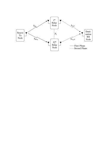
Figure 1: Cooperative DS-CDMA System Model

We also consider the uplink of a cooperative DS-CDMA system with $K$ users, $N_{r}$ relays, $N$ chips per symbol and $L_{p}$ $(L_{p}<N)$ propagation paths for each link. The system shown in 1 is equipped with an AF protocol at each relay. The received signals at the $n^{\mathrm{th}}$ relay and the destination nodes are filtered by a chip-pulse matched filter, sampled at chip rate to obtain sufficient statistics and organized into $M\times 1$ vectors as described by

$$\mathbf{r}_{\mathrm{sr}_{n}}[i]=\sum^{K}_{k=1}a_{\mathrm{s}_{k}}[i]b_{k}[i]h_{\mathrm{sr}_{n}}[i]\mathbf{c}_{k}[i]+\mathbf{n}_{\mathrm{r}_{n}}[i],$$ (3)

$$\mathbf{r}_{\mathrm{rd}}[i]=\sum^{N_{\mathrm{r}}}_{n=1}a_{\mathrm{r}_{n}}[i]h_{\mathrm{r}_{n}\mathrm{d}}[i]\mathbf{r}_{\mathrm{sr}_{n}}[i]+\mathbf{n}_{\mathrm{d}}[i]$$ (4)

and

$$\mathbf{r}_{\mathrm{rd}}[i]=\sum^{N_{\mathrm{r}}}_{n=1}\sum^{K}_{k=1}a_{\mathrm{s}_{k}}[i]a_{\mathrm{r}_{n}}[i]h_{\mathrm{sr}_{n}}[i]h_{\mathrm{r}_{n}\mathrm{d}}[i]\mathbf{c}_{k}[i]b_{k}[i]+\sum^{N_{\mathrm{r}}}_{n=1}a_{\mathrm{r}_{n}}[i]h_{\mathrm{r}_{n}\mathrm{d}}[i]\mathbf{n}_{\mathrm{r}_{n}}[i]+\mathbf{n}_{\mathrm{d}}[i].$$ (5)

where $h_{\mathrm{sr}_{n}}[i]$ and $h_{\mathrm{r}_{n}\mathrm{d}}[i]$ are the channel fading channel coefficients between the source and the $n^{\mathrm{th}}$ relay, and the $n^{\mathrm{th}}$ relay and the destination, respectively, and $\mathbf{n}_{\mathrm{r}_{n}}[i]$ and $\mathbf{n}_{\mathrm{d}}[i]$ are additive white Gaussian noise vectors at the relays and the destination, respectively.

The received data is processed by a linear receive filter, which produces the output given by

$$x[i]={\mathbf{w}}^{H}[i]{\boldsymbol{r}}_{\rm rd}[i],$$ (6)

where ${\mathbf{w}}[i]$ is an $M$-dimensional vector that corresponds to the receive filter for the cooperative system.

III Proposed Bidirectional Scheme

Adaptive parameter estimation has two primary objectives: estimation and tracking of the desired parameters. When applied to multiuser wireless systems, these translate into recovery of the desired symbol, tracking of channel variations and suppression of MUI. However, in fast fading channels these objectives place unrealistic demands on conventional filtering and estimation schemes. Differential techniques reduce these demands by relieving adaptive receivers from the task of tracking fading coefficients [38]. This is achieved by posing an optimization problem where the ratio between two successive received samples is the quantity to be tracked. Such an approach is enabled by the presumption that, although the fading is fast, there is correlation between the adjacent channel samples as described by

$$f_{1}[i]=E\left[h_{1}[i]h_{1}^{\ast}[i+1]\right]\geq 0,\\$$ (7)

where $h_{1}[i]$ is the channel coefficient of the desired user. The interference suppression of the resulting receive filter is improved in fast fading environments compared to conventional adaptive receivers but only the ratio of adjacent fading samples is obtained. Consequently, differential MMSE schemes are suited to differential modulation where the ratio between adjacent symbols is the data carrying mechanism.

However, limiting the optimization to two adjacent samples exposes these processes to the negative effects of uncorrelated samples

$$E\left[h_{1}[i]h_{1}^{\ast}[i+1]\right]\approx 0,$$ (8)

but also does not exploit the correlation that may be present between two or more adjacent samples, i.e.,

$$\begin{array}[]{l}f_{2}[i]=E\left[h_{1}[i]h_{1}^{\ast}[i-1]\right]>0\\ f_{3}[i]=E\left[h_{1}[i+1]h_{1}^{\ast}[i-1]\right]>0.\\ \end{array}$$ (9)

In order to address these weaknesses, we propose a bidirectional MSE cost function based on multiple adjacent samples so that the number of channel scenarios under which the differential MMSE performs beneficial adaptation is substantially increased. Termed the bidirectional MMSE, due to the use of multiple time instants, the motivation behind this proposition is illustrated by the plots of fading/channel coefficients in Fig. 2, where $\mathrm{J}_{1}$ represents the $2$ sample differential MMSE. There is a low level of correlation present between samples $i$ and $i-1$, thus any adaptation of the receive filter will bring little benefit. However, the proposed scheme for $3$ time instants operates over $\mathrm{J}_{1}$,$\mathrm{J}_{2}$ and $\mathrm{J}_{3}$; therefore, it can exploit the correlation between $i+1$ and $i-1$ and past data. Figure 2 gives an example of a channel where there is a significant level of correlation between samples.

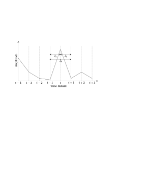
Figure 2: Fading channels: an uncorrelated fading channel on the top figure and a correlated fading channel on the bottom figure.

The proposed bidirectional scheme can be expressed in the form of an an optimization problem as described by

$$\begin{array}[]{lll}\mathbf{w}_{o}[i]=\underset{\mathbf{w}[i]}{\mathrm{arg\;min}}&E\left[\left|b[i]\mathbf{w}^{H}[i]\mathbf{r}[i-1]-b[i-1]\mathbf{w}^{H}[i]\mathbf{r}[i]\right|^{2}\right.\\ &\hskip 91.04872pt\vdots\\ &+\left|b[i]\mathbf{w}^{H}[i]\mathbf{r}[i-(D-1)]-b[i-(D-1)]\mathbf{w}^{H}[i]\mathbf{r}[i]\right|^{2}\\ &\\ &+\left|b[i-1]\mathbf{w}^{H}[i]\mathbf{r}[i-2]-b[i-2]\mathbf{w}^{H}[i]\mathbf{r}[i-1]\right|^{2}\\ &\hskip 91.04872pt\vdots\\ &+\left|b[i-1]\mathbf{w}^{H}[i]\mathbf{r}[i-(D-1)]-b[i-(D-1)]\mathbf{w}^{H}[i]\mathbf{r}[i-1]\right|^{2}\\ &\\ &+\left.\left|b[i-(D-2)]\mathbf{w}^{H}[i]\mathbf{r}[i-(D-1)]-b[i-(D-1)]\mathbf{w}^{H}[i]\mathbf{r}[i-(d-2)]\right|^{2}\right]\\ \end{array},$$ (10)

where $D$ denotes the number of considered time instants. Introducing summations into (10) yields a more concise form

$$\mathbf{w}_{o}[i]=\underset{\mathbf{w}[i]}{\mathrm{arg\;min}}E\left[\displaystyle\sum^{D-2}_{d=0}\sum^{D-1}_{l=d+1}\left|b[i-d]\mathbf{w}^{H}[i]\mathbf{r}[i-l]-b[i-l]\mathbf{w}^{H}[i]\mathbf{r}[i-d]\right|^{2}\right],$$ (11)

where an output power constraint is required to avoid the trivial all-zero receive filter solution

$$E\left[\left|\mathbf{w}^{H}[i]\mathbf{r}[i]\right|^{2}\right]=1.$$ (12)

Although the existing differential scheme operates over $2$ correlated samples, the proposed scheme is able to exploit the additional correlation present between multiple adjacent samples. Moreover, it is also possible to obtain further gain by weighting the correlation between multiple adjacent samples. However, the benefit of using multiple time instant is dependent on the fading rate of the channel and the related correlation of the channel coefficients. We have investigated the use of multiple time instants and it turns out that a scheme which exploits $3$ adjacent samples captures most of the performance benefits. In particular, we have tested the proposed bidirectional scheme and algorithms with various values of adjacent time instants (between 4 and 8) and verified that exploiting extra time instants above 3 does not yield significant gains. In fact, the number of time instants is a parameter to be chosen by the designer.

The optimization problem of the proposed scheme for $3$ time instants is given by

$$\begin{array}[]{lllr}\mathbf{w}_{o}[i]=\underset{\mathbf{w}[i]}{\mathrm{arg\;min}}&E\left[\left|b[i]\mathbf{w}^{H}[i]\mathbf{r}[i-1]-b[i-1]\mathbf{w}^{H}[i]\mathbf{r}[i]\right|^{2}\right.&(\mathrm{J}_{1})\\ &+\left|b[i]\mathbf{w}^{H}[i]\mathbf{r}[i-2]-b[i-2]\mathbf{w}^{H}[i]\mathbf{r}[i]\right|^{2}&(\mathrm{J}_{2})\\ &+\left.\left|b[i-1]\mathbf{w}^{H}[i]\mathbf{r}[i-2]-b[i-2]\mathbf{w}^{H}\mathbf{r}[i-1]\right|^{2}\right]&(\mathrm{J}_{3})\\ \end{array},$$ (13)

where $\mathrm{J}_{1}-\mathrm{J}_{3}$ equate to those of Fig. 2, and the time instants of interest have been altered to avoid the use of future samples. In addition to (LABEL:eq:Bidirectional_Cost_Function), an output power constraint is again required to avoid an all-zero trivial solution as given by

$$E\left[\left|\mathbf{w}^{H}[i]\mathbf{r}[i]\right|^{2}\right]=1.$$ (14)

In what follows, we describe switching and weighting strategies to optimize the proposed scheme and obtain further performance gain.

IV Switching and Weighting Strategies

The advantages of a bidirectional scheme operating over 3 time or more time instants have been verified in our studies. However, the performance of the scheme may be degraded when received vectors based on uncorrelated fading coefficients are employed in the update of the receive filter. This is particulary evident from the example with an uncorrelated channel illustrated in Fig. 2, where the contribution to the cost function represented by $\mathrm{J}_{3}$ is unlikely to aid the accurate adaptation of $\mathbf{w}[i]$. To avoid this we introduce a set of switching or mixing parameters that determine the weighting of the $D$ constituent elements of the bidirectional cost function. The proposed generalized bidirectional cost function with weighting factors is described by

$$\mathbf{w}_{o}[i]=\underset{\mathbf{w}[i]}{\mathrm{arg\;min}}E\left[\displaystyle\sum^{D-2}_{d=0}\sum^{D-1}_{l=d+1}\rho_{n}[i]\left|b[i-d]\mathbf{w}^{H}[i]\mathbf{r}[i-l]-b[i-l]\mathbf{w}^{H}[i]\mathbf{r}[i-d]\right|^{2}\right],$$ (15)

where $n=d(D-3)+l+1$. However, we again focus on the case with $D=3$ in the remainder of this work. With these modifications the proposed bidirectional MSE cost function with $3$-time instand and weighting factors is given by

$$\begin{array}[]{lllr}\mathbf{w}_{o}[i]=\underset{\mathbf{w}[i]}{\mathrm{arg\;min}}&E\left[\rho_{1}[i]\left|b[i]\mathbf{w}^{H}[i]\mathbf{r}[i-1]-b[i-1]\mathbf{w}^{H}[i]\mathbf{r}[i]\right|^{2}\right.&(\mathrm{J}_{1})\\ &+\rho_{2}[i]\left|b[i]\mathbf{w}^{H}[i]\mathbf{r}[i-2]-b[i-2]\mathbf{w}^{H}[i]\mathbf{r}[i]\right|^{2}&(\mathrm{J}_{2})\\ &+\left.\rho_{3}[i]\left|b[i-1]\mathbf{w}^{H}[i]\mathbf{r}[i-2]-b[i-2]\mathbf{w}^{H}[i]\mathbf{r}[i-1]\right|^{2}\right]&(\mathrm{J}_{3})\\ \end{array},$$ (16)

where $0\leq\rho_{n}\leq 3$ for $n=1,2,3$ are the weighting factors.

The determination of the receive vector samples that correspond to the scenarios depicted in Figure 2 is essential if correct optimization of the $\rho$ is to be achieved. The use of CSI to achieve this would be an effective but impractical solution due to the difficulty in obtaining CSI; consequently, other methods must be sought. In this section, we propose the use of two alternative metrics: the signal power differential after interference suppression between the considered time instants, and the error between the considered time instants.

Firstly, we consider a switching scheme where $\rho_{1-3}=[0,1]$ are determined at each time instant based on the following post-filtering power differential metrics:

$$\begin{array}[]{l}P_{1}[i]=\left|\mathbf{w}[i]^{H}\mathbf{r}[i]\right|^{2}-\left|\mathbf{w}[i]^{H}\mathbf{r}[i-1]\right|^{2}\\ P_{2}[i]=\left|\mathbf{w}[i]^{H}\mathbf{r}[i]\right|^{2}-\left|\mathbf{w}[i]^{H}\mathbf{r}[i-2]\right|^{2}\\ P_{3}[i]=\left|\mathbf{w}[i]^{H}\mathbf{r}[i-1]\right|^{2}-\left|\mathbf{w}[i]^{H}\mathbf{r}[i-2]\right|^{2}.\\ \end{array}$$ (17)

If the power difference for each of $\mathrm{J}_{1-3}$ exceeds a predefined threshold, the corresponding $\rho$ is set to zero; therefore, removing the corresponding element of the cost function from the adaptation process at that time instant. For highly dynamic channels one requires an adaptive threshold which is able to track the changes in the system and determine appropriate time instants based on successive samples. Consequently, for each $\rho_{n}$ a threshold, $T_{n}[i]$, related to a time-averaged, windowed, root-mean-square of the relevant differential power is used. The value of $\rho_{n}$ in then determined in the following manner:

$$\rho_{n}[i]=\left\{\begin{array}[]{ll}0&\mathrm{if}~{}P_{n}[i]\geq T_{n}[i]\\ 1&\mathrm{otherwise}\\ \end{array},\right.$$ (18)

where

$$T_{n}[i]=\nu\left[\lambda_{P}P_{n_{RMS}}[i]+(1-\lambda_{P})P_{n_{RMS}}[i]\right],$$ (19)

$$P_{n_{RMS}}[i]=\sqrt{\frac{1}{m-1}\sum^{i}_{l=i-m}P_{n}[l]^{2}},$$ (20)

and $\nu$ is a positive user defined constant greater than unity that scales the threshold. The threshold $\nu$ is set with the help of computer experiments in a similar way as the step size of the NLMS algorithm is tuned. The aim is to scale the threshold such that it will be used to inform the algorithm about the relevant differential power which should be used.

Although the current sample corresponding to $\mathrm{J}_{n}$ may bring little benefit in terms of adaptation, this does not indicate that all previous cost function elements corresponding to $\mathrm{J}_{n}$ should be discarded. An alternative approach is to use a set of convex mixing parameters that are not restricted to 1 or 0. This allows each element of the cost function to be more precisely weighted based on its previous and current values. However, the setting of these mixing parameters is once again problematic if they are fixed. Accordingly, an adaptive implementation that can take account of the time-varying channels and previous values which continue to have an impact on the adaptation of the filter is sought. The errors extracted from the cost function (LABEL:eq:Bidirectional_Cost_Function_Switching) are chosen as the metric for developing algorithms. These provide an input to the weighting factor calculation process that is directly related to the cost function of (LABEL:eq:Bidirectional_Cost_Function_Switching). The time-varying mixing factors are given by

$$\rho_{n}[i]=\lambda_{e}\rho_{n}[i-1]+(1-\lambda_{e})\frac{e_{T}[i]-|e_{n}[i]|}{e_{T}[i]}$$ (21)

where

$$e_{T}[i]=|e_{1}[i]|+|e_{2}[i]|+|e_{3}[i]|,$$ (22)

and the individual error terms are calculated as

$$\begin{array}[]{l}e_{1}[i]=b[i]\mathbf{w}^{H}[i-1]\mathbf{r}[i-1]-b[i-1]\mathbf{w}^{H}[i-1]\mathbf{r}[i]\\ e_{2}[i]=b[i]\mathbf{w}^{H}[i-1]\mathbf{r}[i-2]-b[i-2]\mathbf{w}^{H}[i-1]\mathbf{r}[i]\\ e_{3}[i]=b[i-1]\mathbf{w}^{H}[i-1]\mathbf{r}[i-2]-b[i-2]\mathbf{w}^{H}[i-1]\mathbf{r}[i-1].\\ \end{array}$$ (23)

The forgetting factor, $0\leq\lambda_{e}\leq 1$, is user defined and, along with normalization by the total error, $e_{T}[i]$, and $\displaystyle{\sum^{3}_{n=1}}\rho_{n}[0]=1$, ensures $\displaystyle{\sum^{3}_{n=1}}\rho_{n}[i]=1$ and a convex combination at each time instant.

V Adaptive Algorithms

In order to devise low-complexity adaptive algorithms based on the proposed bidirectional schemes, we consider the minimization of the cost function given by

$$\begin{array}[]{ll}C(\mathbf{w}[i])=&E\left[\left|b[i]\mathbf{w}^{H}[i-1]\mathbf{r}[i-1]-b[i-1]\mathbf{w}^{H}[i]\mathbf{r}[i]\right|^{2}\right.\\ &+\left|b[i]\mathbf{w}^{H}[i-2]\mathbf{r}[i-2]-b[i-2]\mathbf{w}^{H}[i]\mathbf{r}[i]\right|^{2}\\ &+\left.\left|b[i-1]\mathbf{w}^{H}[i-2]\mathbf{r}[i-2]-b[i-2]\mathbf{w}^{H}[i]\mathbf{r}[i-1]\right|^{2}\right]\\ &\\ \mathrm{subject\,to}&E\left[\left|\mathbf{w}[i]^{H}\mathbf{r}[i]\right|^{2}\right]=1.\end{array}$$ (24)

This cost function then forms the basis of the adaptive algorithms derived in this section. However, to reduce the complexity of the derivations, enforcement of the non-zero constraint is not included and instead enforced in a stochastic manner at each time instant after the adaptation step is complete [38].

V-A Normalized Least-Mean Square Algorithm

We begin with the low-complexity NLMS implementation that employs an instantaneous gradient in a steepest descent framework. Firstly, the instantaneous gradient of (24) is taken with respect to $\mathbf{w}^{*}[i]$, yielding

$$\begin{array}[]{ll}\nabla_{\mathbf{w}^{*}[i]}C(\mathbf{w}[i])=&-b[i-1]\mathbf{r}[i](b[i]\mathbf{w}^{H}[i-1]\mathbf{r}[i-1]-b[i-1]\mathbf{w}^{H}[i]\mathbf{r}[i])^{H}\\ &-b[i-2]\mathbf{r}[i](b[i]\mathbf{w}^{H}[i-2]\mathbf{r}[i-2]-b[i-2]\mathbf{w}^{H}[i]\mathbf{r}[i])^{H}\\ &-b[i-2]\mathbf{r}[i-1](b[i-1]\mathbf{w}^{H}[i-2]\mathbf{r}[i-2]-b[i-2]\mathbf{w}^{H}[i]\mathbf{r}[i-1])^{H}\end{array}$$ (25)

At this point, in order to improve the convergence performance of the NLMS algorithm, the bracketed error terms of (25) are modified by replacing the receive filters with the most recently calculated one, $\mathbf{w}[i-1]$. The resulting gradient expression is given by

$$\begin{array}[]{ll}\nabla_{\mathbf{w}^{*}[i]}C(\mathbf{w}[i])=&-b[i-1]\mathbf{r}[i]\underbrace{\left(b[i]\mathbf{w}^{H}[i-1]\mathbf{r}[i-1]-b[i-1]\mathbf{w}^{H}[i-1]\mathbf{r}[i]\right)^{H}}_{e_{1}[i]}\\ &-b[i-2]\mathbf{r}[i]\underbrace{\left(b[i]\mathbf{w}^{H}[i-1]\mathbf{r}[i-2]-b[i-2]\mathbf{w}^{H}[i-1]\mathbf{r}[i]\right)^{H}}_{e_{2}[i]}\\ &-b[i-2]\mathbf{r}[i-1]\underbrace{\left(b[i-1]\mathbf{w}^{H}[i-1]\mathbf{r}[i-2]-b[i-2]\mathbf{w}^{H}[i-1]\mathbf{r}[i-1]\right)^{H}}_{e_{3}[i]}\end{array}.$$ (26)

Placing the above gradient expression in the steepest descent update recursion, we obtain

$$\mathbf{w}[i]=\mathbf{w}[i-1]+\frac{\mu}{M[i]|\mathbf{w}^{H}[i-1]\mathbf{r}[i-1]|}\left[b[i-1]\mathbf{r}[i]e_{1}^{\ast}[i]+b[i-2]\mathbf{r}[i]e_{2}^{\ast}[i]+b[i-2]\mathbf{r}[i-1]e_{3}^{\ast}[i]\right],$$ (27)

where $\mu$ is the step-size and the normalization factor, $M[i]$, is given by

$$M[i]=\lambda_{M}M[i-1]+(1-\lambda_{M})\mathbf{r}^{H}[i]\mathbf{r}[i],$$ (28)

where $\lambda_{M}$ is an exponential forgetting factor [38]. The enforcement of the constraint is performed by the denominator of (27) which ensures that the receive filter $\mathbf{w}[i]$ does not tend towards a zero correlator as the adaptation progresses.

The incorporation of the variable switching and mixing factors of Section IV has the potential to improve the performance of the above algorithm by optimizing the weighting of the error terms of (26). Integration of the factors given by (18) and (21) yields

$$\mathbf{w}[i]=\mathbf{w}[i-1]+\frac{\mu}{M[i]|\mathbf{w}^{H}[i-1]\mathbf{r}[i-1]|}\left[\rho_{1}[i]b[i-1]\mathbf{r}[i]e_{1}[i]+\rho_{2}[i]b[i-2]\mathbf{r}[i]e_{2}[i]+\rho_{3}[i]b[i-2]\mathbf{r}[i-1]e_{3}[i]\right]$$ (29)

as the receive filter update equation.

V-B Least Squares Algorithm

To achieve faster convergence and increased robustness to fading we now pursue a LS based solution. Firstly, the bidirectional cost function of (24) is cast as an LS problem by replacing the expected value with a weighted summation, as described by

$$\begin{array}[]{llll}C_{\rm LS}(\mathbf{w}[i])&=\displaystyle{\sum^{i}_{l=1}}&\lambda^{i-l}&\left[\left|b[i]\mathbf{w}^{H}[i-1]\mathbf{r}[i-1]-b[i-1]\mathbf{w}^{H}[i]\mathbf{r}[i]\right|^{2}+\right.\\ &&&\left|b[i]\mathbf{w}^{H}[i-2]\mathbf{r}[i-2]-b[i-2]\mathbf{w}^{H}[i]\mathbf{r}[i]\right|^{2}+\\ &&&\left.\left|b[i-1]\mathbf{w}^{H}[i-2]\mathbf{r}[i-2]-b[i-2]\mathbf{w}^{H}[i-1]\mathbf{r}[i-1]\right|^{2}\right]\\ \end{array},$$ (30)

where $\lambda$ is an exponential forgetting factor. Proceeding as with the conventional LS derivation, and modifying the equivalent error terms in a similar manner to as in (26), we arrive at the following expressions for the component autocorrelation matrices:

$$\begin{array}[]{l}\bar{\mathbf{R}}_{1}[i]=\lambda\bar{\mathbf{R}}_{1}[i-1]+b[i-1]\mathbf{r}[i]\mathbf{r}^{H}[i]b^{\ast}[i-1]\\ \bar{\mathbf{R}}_{2}[i]=\lambda\bar{\mathbf{R}}_{2}[i-1]+b[i-2]\mathbf{r}[i]\mathbf{r}^{H}[i]b^{\ast}[i-2]\\ \bar{\mathbf{R}}_{3}[i]=\lambda\bar{\mathbf{R}}_{3}[i-1]+b[i-2]\mathbf{r}[i-1]\mathbf{r}^{H}[i-1]b^{\ast}[i-2]\\ \end{array}$$ (31)

and the component cross-correlation vectors:

$$\begin{array}[]{l}\bar{\mathbf{t}}_{1}[i]=\lambda\bar{\mathbf{t}}_{3}[i-1]+b[i-1]\mathbf{r}[i]\mathbf{r}^{H}[i-1]\mathbf{w}[i-1]b^{\ast}[i]\\ \bar{\mathbf{t}}_{2}[i]=\lambda\bar{\mathbf{t}}_{2}[i-1]+b[i-2]\mathbf{r}[i]\mathbf{r}^{H}[i-2]\mathbf{w}[i-1]b^{\ast}[i]\\ \bar{\mathbf{t}}_{3}[i]=\lambda\bar{\mathbf{t}}_{3}[i-1]+b[i-2]\mathbf{r}[i-1]\mathbf{r}^{H}[i-2]\mathbf{w}[i-1]b^{\ast}[i-1]\\ \end{array}.$$ (32)

The overall correlation structure is then formed from the summation of the preceding expressions, yielding

$$\bar{\mathbf{R}}[i]=\bar{\mathbf{R}}_{1}[i]+\bar{\mathbf{R}}_{2}[i]+\bar{\mathbf{R}}_{3}[i]$$ (33)

and

$$\bar{\mathbf{t}}[i]=\bar{\mathbf{t}}_{1}[i]+\bar{\mathbf{t}}_{2}[i]+\bar{\mathbf{t}}_{3}[i].$$ (34)

where

$$\mathbf{w}[i]=\bar{\mathbf{R}}^{-1}[i]\bar{\mathbf{t}}[i].$$ (35)

Similarly to the NLMS algorithm, performance improvements can be expected if the variable switching and mixing factors, (18) and (21), are incorporated into the correlation expressions. The resulting expressions are

$$\mathbf{R}[i]=\rho_{1}[i]\mathbf{R}_{1}[i]+\rho_{2}[i]\mathbf{R}_{2}[i]+\rho_{3}[i]\mathbf{R}_{3}[i]$$ (36)

$$\mathbf{t}[i]=\rho_{1}[i]\mathbf{t}_{1}[i]+\rho_{2}[i]\mathbf{t}_{2}[i]+\rho_{3}[i]\mathbf{t}_{3}[i]$$ (37)

Introducing the above expression into the RLS framework would lead to a low-complexity algorithm with improved convergence and robustness compared to the NLMS of Section V-A. This requires the integration of (31) with the matrix inversion lemma [13, 41]. However, the derivation requires an expression with a rank-$1$ update of the form

$$\mathbf{R}[i]=\mathbf{R}[i-1]+\lambda\mathbf{r}[i]\mathbf{r}^{H}[i]$$ (38)

for the autocorrelation matrix; a form which (31) is unable to fit into without assumptions that cause a significant performance degradation. Consequently, an alternative low-complexity algorithm to implement the LS solution given by (31) - (35) is required.

V-C Conjugate Gradient Algorithm

Due to the particular form of the bidirectional LS formulation and the conventional RLS recursion, an alternative low-complexity method is now derived. The CG technique has been chosen to avoid matrix inversions and due to its excellent convergence properties [42, 43, 44]. We begin the derivation of the proposed CG type algorithm with the autocorrelation (31) and cross-correlation (32) structures of subsection V-B. Inserting them into the standard CG quadratic form yields

$$J(\mathbf{w})=\mathbf{w}^{H}[i]\mathbf{R}[i]\mathbf{w}[i]-\mathbf{t}^{H}[i]\mathbf{w}[i].$$ (39)

From [43], the unique minimiser of (39) is also the minimiser of

$$\mathbf{R}[i]\mathbf{w}[i]=\mathbf{t}[i].$$ (40)

This shows the suitability of the CG algorithm to the bidirectional problem. At each time instant a number of iterations of the following method are required to reach an accurate solution, where the iterations are indexed with the variable $j$. Other single iteration CG methods are available but these depend upon degeneracy - a term that describes the situation where the successive CG vectors are not orthogonal [45]. Consequently, we employ the conventional method to ensure satisfactory convergence. At the $i^{\mathrm{th}}$ time instant the gradient and direction vectors are initialized as

$$\mathbf{g}_{0}[i]=\nabla_{\mathbf{w}[i]}C_{\rm LS}(\mathbf{w}[i])=\mathbf{R}[i]\mathbf{w}_{0}[i]-\mathbf{t}[i]$$ (41)

and

$$\mathbf{d}_{0}[i]=-\mathbf{g}_{0}[i],$$ (42)

respectively, where the gradient expression is equivalent to those used in the derivation of the previous algorithms. The vectors $\mathbf{d}_{j}[i]$ and $\mathbf{d}_{j+1}[i]$ are $\mathbf{R}[i]$ orthogonal with respect to $\mathbf{R}[i]$ such that $\mathbf{d}_{j}[i]\mathbf{R}[i]\mathbf{d}_{l}[i]=0$ for $j\neq l$. At each iteration, the receive filter is updated as

$$\mathbf{w}_{j+1}[i]=\mathbf{w}_{j}[i]+\alpha_{j}[i]\mathbf{d}_{j}[i]$$ (43)

where $\alpha_{j}[i]$ is the minimizer of $J(\mathbf{w}_{j+1}[i])$ such that

$$\alpha_{j}=\frac{-\mathbf{d}_{j}^{H}\mathbf{g}_{j}[i]}{\mathbf{d}_{j}^{H}[i]\mathbf{R}[i]\mathbf{d}_{j}[i]}.$$ (44)

The gradient vector is then updated according to

$$\mathbf{g}_{j+1}[i]=\mathbf{R}[i]\mathbf{w}_{j}[i]-\mathbf{t}[i]$$ (45)

and a new conjugate gradient direction vector is obtained as given by

$$\mathbf{d}_{j+1}[i]=-\mathbf{g}_{j+1}[i]+\beta_{j}[i]\mathbf{d}_{j}[i]$$ (46)

where

$$\beta_{j}[i]=\frac{\mathbf{g}_{j+1}^{H}[i]\mathbf{R}[i]\mathbf{d}_{j}[i]}{\mathbf{d}_{j}^{H}[i]\mathbf{R}[i]\mathbf{d}_{j}[i]}$$ (47)

ensures the $\mathbf{R}[i]$ orthogonality between $\mathbf{d}_{j}[i]$ and $\mathbf{d}_{l}[i]$ where $j\neq l$. The iterations (43) - (47) are then repeated until $j=j_{max}$.

The variable switching and mixing factors can be incorporated into the algorithm to improve performance. This is achieved by operating the CG algorithm over the modified correlation structures given by (36) and (37).

VI Analysis

In this section, we analyze the proposed bidirectional algorithms to gain insight of the expected performance but also to obtain further knowledge into the operation of the proposed and existing algorithms. The unconventional form of the proposed cost functions precludes the application of standard MSE analysis. Consequently, we concentrate on the signal-to-interference-plus-noise ratio (SINR) of the proposed algorithms in order to analyze their interference suppression and tracking performance. We firstly study the NLMS algorithm and the features of its weight error correlation matrix in order to arrive at an analytical SINR expression. Following this, we explore the analogy between the form of the bidirectional expression and convex combinations of adaptive receive filters [46, 47].

VI-A SINR Analysis

Let us define the instantaneous SINR expression given by

$$\mathrm{SINR}_{\rm inst}\triangleq\frac{\mathbf{w}^{H}[i]\mathbf{R}_{\mathrm{S}}\mathbf{w}[i]}{\mathbf{w}^{H}[i]\mathbf{R}_{\mathrm{I}}\mathbf{w}[i]},$$ (48)

where $\mathbf{R}_{S}$ and $\mathbf{R}_{I}$ are the signal and interference and noise correlation matrices, into a form amenable to analysis.

The receive filter error weight vector is described by

$${\boldsymbol{\varepsilon}}[i]=\mathbf{w}[i]-\mathbf{w}_{o}[i],$$ (49)

where $\mathbf{w}_{o}$ is the instantaneous standard MMSE receiver.

Let us now describe the expression of the numerator of (48) with the desired signal component:

$$\mathrm{S}_{\rm c}=\boldsymbol{\varepsilon}^{H}[i]\mathbf{R}_{\mathrm{S}}\boldsymbol{\varepsilon}[i]+\boldsymbol{\varepsilon}^{H}[i]\mathbf{R}_{\mathrm{S}}\mathbf{w}_{o}[i]+\overbrace{\mathbf{w}_{o}^{H}[i]\mathbf{R}_{\mathrm{S}}\mathbf{w}_{o}[i]}^{P_{\mathrm{S,opt}}[i]}+\mathbf{w}_{o}^{H}[i]\mathbf{R}_{\mathrm{S}}\boldsymbol{\varepsilon}[i],$$ (50)

and of the interference plus noise component described by

$$\mathrm{S}_{i+n}=\boldsymbol{\varepsilon}^{H}[i]\mathbf{R}_{\mathrm{I}}\boldsymbol{\varepsilon}[i]+\boldsymbol{\varepsilon}^{H}[i]\mathbf{R}_{\mathrm{I}}\mathbf{w}_{o}[i]+\underbrace{\mathbf{w}_{o}^{H}[i]\mathbf{R}_{\mathrm{I}}\mathbf{w}_{o}[i]}_{P_{\mathrm{I,opt}}[i]}+{\mathbf{w}}_{o}^{H}[i]{\mathbf{R}}_{\mathrm{I}}{\boldsymbol{\varepsilon}}[i].$$ (51)

Taking the expectation and the trace of $\mathrm{S}_{c}$ and $\mathrm{S}_{i+n}$, defining $\mathbf{K}[i]=E[\boldsymbol{\varepsilon}[i]\boldsymbol{\varepsilon}^{H}[i]]$ and $\mathbf{G}[i]=E[\mathbf{w}_{o}[i]\boldsymbol{\varepsilon}^{H}[i]]$, we can define the following SINR expression:

$$\begin{split}\mathrm{SINR}&\triangleq\frac{{\rm tr}\{E[S_{c}]\}}{{\rm tr}\{E[S_{i+n}]\}}\\ &=\frac{{\rm tr}[\mathbf{K}[i]\mathbf{R}_{\mathrm{S}}+\mathbf{G}[i]\mathbf{R}_{\mathrm{S}}+P_{\mathrm{S,opt}}[i]+\mathbf{G}^{H}[i]\mathbf{R}_{\mathrm{S}}]}{{\rm tr}[\mathbf{K}[i]\mathbf{R}_{\mathrm{I}}+\mathbf{G}[i]\mathbf{R}_{\mathrm{I}}+P_{\mathrm{I,opt}}[i]+\mathbf{G}^{H}[i]\mathbf{R}_{\mathrm{I}}]}.\end{split}$$ (52)

From (52) it is clear that we need to pursue expressions for $\mathbf{K}[i]$ and $\mathbf{G}[i]$ in order to reach an analytical interpretation of the bidirectional NLMS scheme.

Substituting the filter error weight vector into the filter update expression of (27) yields a recursive expression for the receive filter error weight vector described by

$$\begin{array}[]{ll}\boldsymbol{\varepsilon}[i]&=\boldsymbol{\varepsilon}[i-1]\\ &+\left[\mathbf{I}+\mu\mathbf{r}[i]b[i-1]\mathbf{r}^{H}[i-1]b^{\ast}[i]-\mu\mathbf{r}[i]b[i-1]\mathbf{r}^{H}[n]b^{\ast}[i-1]\right.\\ &+\mu\mathbf{r}[i]b[i-2]\mathbf{r}^{H}[i-2]b^{\ast}[i]-\mu\mathbf{r}[i]b[i-2]\mathbf{r}^{H}[n]b^{\ast}[i-2]\\ &\left.+\mu\mathbf{r}[i-1]b[i-2]\mathbf{r}^{H}[i-2]b^{\ast}[i-1]-\mu\mathbf{r}[i-1]b[i-2]\mathbf{r}^{H}[i-1]b^{\ast}[i-2]\right]\boldsymbol{\varepsilon}[i-1]\\ &+\mu\mathbf{r}[i]b[i-1]e^{\ast}_{o,1}[i]\\ &+\mu\mathbf{r}[i]b[i-2]e^{\ast}_{o,2}[i]\\ &+\mu\mathbf{r}[i-1]b[i-2]e^{\ast}_{o,3}[i]\\ \end{array},$$ (53)

where the terms $e_{o,1-3}$ denote the error terms of (26) when the optimum filter $\mathbf{w}_{o}$ is used. Utilizing the direct averaging approach developed by Kushner [48], often invoked in this type of stochastic analysis, the solution to the stochastic difference equation of (53) can be approximated by the solution to a second equation [13, 49], such that

$$\begin{array}[]{l}E\left[\mathbf{I}+\mu\mathbf{r}[i]b[i-1]\mathbf{r}^{H}[i-1]b^{\ast}[i]-\mu\mathbf{r}[i]b[i-1]\mathbf{r}^{H}[n]b^{\ast}[i-1]\right.\\ +\mu\mathbf{r}[i]b[i-2]\mathbf{r}^{H}[i-2]b^{\ast}[i]-\mu\mathbf{r}[i]b[i-2]\mathbf{r}^{H}[n]b^{\ast}[i-2]\\ \left.+\mu\mathbf{r}[i-1]b[i-2]\mathbf{r}^{H}[i-2]b^{\ast}[i-1]-\mu\mathbf{r}[i-1]b[i-2]\mathbf{r}^{H}[i-1]b^{\ast}[i-2]\right]\\ =\\ \mathbf{I}+\mu\mathbf{F}_{1}-\mu\mathbf{R}_{1}+\mu\mathbf{F}_{2}-\mu\mathbf{R}_{2}+\mu\mathbf{F}_{3}-\mu\mathbf{R}_{3}\end{array},$$ (54)

where $\mathbf{F}$ and $\mathbf{R}$ are correlations matrices. Specifically, $\mathbf{R}_{1-3}$ are autocorrelation matrices given by

$$\begin{array}[]{l}\mathbf{R}_{1}=E\left[\mu\mathbf{r}[i]b^{\ast}[i-1]\mathbf{r}^{H}[i]b^{\ast}[i-1]\right]\\ \mathbf{R}_{2}=E\left[\mu\mathbf{r}[i]b^{\ast}[i-2]\mathbf{r}^{H}[i]b^{\ast}[i-2]\right]\\ \mathbf{R}_{3}=E\left[\mu\mathbf{r}[i-1]b^{\ast}[i-2]\mathbf{r}^{H}[i-1]b^{\ast}[i-1]\right]\\ \end{array}$$ (55)

and $\mathbf{F}_{1-3}$ cross-time instant correlation matrices, given by

$$\begin{array}[]{l}\mathbf{F}_{1}=E\left[\mu\mathbf{r}[i]b^{\ast}[i-1]\mathbf{r}^{H}[i-1]b^{\ast}[i]\right]\\ \mathbf{F}_{2}=E\left[\mu\mathbf{r}[i]b^{\ast}[i-2]\mathbf{r}^{H}[i-2]b^{\ast}[i]\right]\\ \mathbf{F}_{3}=E\left[\mu\mathbf{r}[i-1]b^{\ast}[i-2]\mathbf{r}^{H}[i-2]b^{\ast}[i-1]\right].\\ \end{array}$$ (56)

Using (54) and the independence assumption of $E\left[e_{o,1-3}[i]\boldsymbol{\varepsilon}[i]\right]=0$, $E\left[\mathbf{r}^{H}[i]\mathbf{r}[i-1]\right]=0$ and $E\left[b_{k}[i]b_{k}[i-1]\right]=0$, we arrive at the expression for $\mathbf{K}[i]$

$$\begin{array}[]{ll}\mathbf{K}[i]=&\left[\mathbf{I}+\mu\mathbf{F}_{1}-\mu\mathbf{R}_{1}+\mu\mathbf{F}_{2}-\mu\mathbf{R}_{2}+\mu\mathbf{F}_{3}-\mu\mathbf{R}_{3}\right]\mathbf{K}[i-1]\left[\mathbf{I}+\mu\mathbf{F}_{1}-\mu\mathbf{R}_{1}+\mu\mathbf{F}_{2}-\mu\mathbf{R}_{2}+\mu\mathbf{F}_{3}-\mu\mathbf{R}_{3}\right]\\ &+\mu^{2}\mathbf{R}_{1}J_{min,1}[i]\\ &+\mu^{2}\mathbf{R}_{2}J_{min,2}[i]\\ &+\mu^{2}\mathbf{R}_{1}J_{min,3}[i]\\ \end{array}$$ (57)

where $J_{{\rm min},j}[i]=|e_{o,j}|^{2}$. Following a similar method, an expression for $\mathbf{G}[i]$ can also be reached

$$\mathbf{G}[i]=\mathbf{G}[i-1]\left[\mu\mathbf{F}_{1}-\mu\mathbf{R}_{1}+\mu\mathbf{F}_{2}-\mu\mathbf{R}_{2}+\mu\mathbf{F}_{3}-\mu\mathbf{R}_{3}\right].$$ (58)

At this point we study the derived expression to gain an insight into the operation of the bidirectional algorithm and the origins of its advantages over the conventional differential scheme. Equivalent expressions for the conventional stochastic gradient scheme are given by

$$\begin{array}[]{ll}\mathbf{K}[i]=&\left[\mathbf{I}+\mu\mathbf{F}_{1}-\mu\mathbf{R}_{1}\right]\mathbf{K}[i-1]\left[\mathbf{I}+\mu\mathbf{F}_{1}-\mu\mathbf{R}_{1}\right]\\ &+\mu^{2}\mathbf{R}_{1}J_{min,1}[i]\\ \mathbf{G}[i]=&\mathbf{G}[i-1]\left[\mu\mathbf{F}_{1}-\mu\mathbf{R}_{1}\right].\end{array}$$ (59)

The bidirectional scheme has a number of additional correlation terms compared to the conventional scheme. Evaluating the cross-time instant matrices yields

$$\begin{array}[]{l}\mathbf{F}_{1}=|a_{1}|^{2}\mathbf{c}_{1}\mathbf{c}_{1}^{H}\underbrace{E\left[h[i]h^{\ast}[i-1]\right]}_{f_{1}[i]}\\ \mathbf{F}_{2}=|a_{1}|^{2}\mathbf{c}_{1}\mathbf{c}_{1}^{H}\underbrace{E\left[h[i]h^{\ast}[i-2]\right]}_{f_{2}[i]}\\ \mathbf{F}_{3}=|a_{1}|^{2}\mathbf{c}_{1}\mathbf{c}_{1}^{H}\underbrace{E\left[h[i-1]h^{\ast}[i-2]\right]}_{f_{3}[i]}\\ \end{array}.$$ (60)

From the expression above it is clear that the underlying factor that governs the SINR performance of the algorithms is the correlation between the considered time instants, $f_{1-3}$, data-ruse and the use of $f_{2}$. Accordingly, it is the additional correlation factors that the proposed bidirectional algorithms possess that enhances its performance compared to the conventional scheme, confirming the initial motivation behind the proposition of the bidirectional approach. Lastly, the $f_{1-3}$ expressions of (60) are the factors that influence the optimum number of considered time instants.

VI-B Combinations of Adaptive Receive Filters

To further our understanding of the bidirectional algorithms we follow a heuristic and complementary approach that leads to an analogy with a combination of adaptive filters [46]. The bidirectional LS solution given by (35) is made up of $6$ constituent correlation structures that result in a filter output of

$$y[i]=\left[\left(\rho_{1}\mathbf{R}_{1}[i]+\rho_{3}\mathbf{R}_{2}[i]+\rho_{3}\mathbf{R}_{3}[i]\right)^{-1}\left(\rho_{1}\mathbf{t}_{1}[i]+\rho_{2}\mathbf{t}_{2}[i]+\rho_{3}\mathbf{t}_{3}[i]\right)\right]^{H}\mathbf{r}[i].$$ (61)

Decomposing the expression above leads us to an expression where the signal $y[i]$ is formed from the output of 3 individual adaptive receive filters

$$\begin{array}[]{ll}y[i]&=\left[\left(\mathbf{R}_{1}[i]+\frac{\rho_{2}}{\rho_{1}}\mathbf{R}_{2}[i]+\frac{\rho_{3}}{\rho_{1}}\mathbf{R}_{3}[i]\right)^{-1}\mathbf{t}_{1}[i]\right]^{H}\mathbf{r}[i]\\ &\\ &+\left[\left(\mathbf{R}_{1}[i]+\frac{\rho_{1}}{\rho_{2}}\mathbf{R}_{2}[i]+\frac{\rho_{3}}{\rho_{2}}\mathbf{R}_{3}[i]\right)^{-1}\mathbf{t}_{2}[i]\right]^{H}\mathbf{r}[i]\\ &\\ &+\left[\left(\mathbf{R}_{1}[i]+\frac{\rho_{1}}{\rho_{3}}\mathbf{R}_{2}[i]+\frac{\rho_{2}}{\rho_{3}}\mathbf{R}_{3}[i]\right)^{-1}\mathbf{t}_{3}[i]\right]^{H}\mathbf{r}[i]\\ \end{array}.$$ (62)

This is equivalent to a convex combination of adaptive receive filters with varying $\lambda$ [46, 47], where each of the 3 filters focuses on the correlation between the 2 of the 3 considered time instants. However, the presence of the autocorrelation matrices in the inverses of the expression also indicates that the remaining time instants also influence the structure of each filter. Although the mixing factors are not separable we can interpret them as a form of weighting that is present in conventional combinations of adaptive filters. This explains in part the additional control and performance they provide.

VII Simulations

In this section, the proposed bidirectional adaptive algorithms are applied to conventional multiuser and cooperative DS-CDMA systems using the signal models described in Section II. The application of the proposed algorithms to multiple-antenna and multi-carrier systems is straightforward and requires a change in the signal models. The individual Rayleigh fading channel coefficients, $h[i]$, are generated using Clarke’s model [50] where 20 scatterers are assumed. In all simulations the number of packets is denoted by $N_{p}$ and the fading rate is given by the dimensionless normalized fading parameter, $T_{s}f_{d}$, where $T_{s}$ is the symbol period and $f_{d}$ is the Doppler frequency shift. The convergence parameters of the algorithms have been optimized resulting in step-sizes forgetting factors of 0.1 and 0.99, respectively, $\lambda_{\mathrm{e}}=0.95$, $\lambda_{M}=0.99$ and the number of CG iterations, $j_{\mathrm{max}}=5$.

As detailed in Section VI, the proposed algorithms do not minimize the same MSE as a conventional MMSE receiver; therefore, the MSE is not an adequate performance metric. As a result, BER and SINR based metrics are chosen for the purpose of comparison between existing algorithms and the optimum MMSE solution. Due to the rapidly fading channel, the instantaneous SNR, $\mathrm{SNR}_{\mathrm{i}}$, is highly variable and so the SINR alone is also not a satisfactory metric. To overcome this it is normalized by the instantaneous SNR to give $\frac{SINR}{SNR_{\mathrm{i}}}$. This value is negative in all simulations and directly reflects the MUI interference suppression and tracking capabilities of the proposed algorithms [39, 38].

VII-A Conventional DS-CDMA

Here we apply the adaptive algorithms of Section V to interference suppression in the uplink of a multiuser DS-CDMA system described in Section II. Each simulation is averaged over $N_{p}$ packets and detailed parameters are specified in each plot.

VII-A1 Analytical Results

We first assess the analytical expressions derived in Section VI-A and their agreement with simulated results. Central to the performance of the differential and bidirectional schemes are the correlation factors $f_{1-3}$ and the related assumption of $h_{1}[i]\approx h_{1}[i-1]$. Examining the effect of the fading rate on the value of $f_{1-3}$ shows that $f_{1}\approx f_{2}\approx f_{3}$ at fading rates of up to $T_{s}f_{d}=0.01$. Consequently, after a large number of received symbols with high total receive power

$$3\left[\mathbf{I}+\mu\mathbf{F}_{1}-\mu\mathbf{R}_{1}\right]\approx\left[\mathbf{I}+\mu\mathbf{F}_{1}-\mu\mathbf{R}_{1}+\mu\mathbf{F}_{2}-\mu\mathbf{R}_{2}+\mu\mathbf{F}_{3}-\mu\mathbf{R}_{3}\right],$$ (63)

due to the decreasing significance of the identity matrix. This indicates that the expected value of the SINR, of the bidirectional scheme, once $f_{1}\approx f_{2}\approx f_{3}$ have stabilised, should be similar to the differential scheme. A second implication is that the bidirectional scheme should converge towards the MMSE level due to the equivalence between the differential scheme and the MMSE solution [38]. Fig. 3 illustrates the analytical performance using the expressions given in Section VI-A.

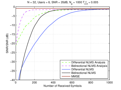
Figure 3: SINR performance comparison of simulated and analytical proposed NLMS algorithms over a single path channel.

The correlation matrices are calculated via ensemble averages prior to the start of the algorithm and $\mathbf{G}[0]=\mathbf{K}[0]=\mathbf{I}$. In Fig. 3 one can see the convergence of the simulated schemes to the analytical and MMSE plots, validating the presented analysis. Due to the highly dynamic nature of the channel, using the expected values of the correlation matrix alone cannot capture the true transient performance of the algorithms. However, the convergence period of the analytical plots within the first 200 iterations can be considered to be within the coherence time and therefore give an indication of the transient performance relative to other analytical plots. Using this justification and the aforementioned analysis, advantages should be present in the transient phase due to the additional correlation information supplied by $\mathbf{F}_{2}$ and $\mathbf{F}_{3}$. This conclusion is supported by Fig. 3 and the similar forms of the analytical and simulated schemes relative to each other and their subsequent convergence.

VII-A2 SINR Performance

The SINR/SNR performance of the proposed algorithms is given by Figs. 4 and 5. The performance of the CG implementation of the differential algorithm is marginally below that of the RLS during convergence but the bidirectional scheme provides noticeable improvements. The differential and bidirectional algorithms converge close to the MMSE optimum as expected from the previous analysis. The bidirectional NLMS algorithm provides more significant improvements over the differential scheme, both in the final stages of convergence and steady-state. These differences can be accounted for by the reduced receive signal power; the matrices equivalent to $\mathbf{F}2$ and $\mathbf{F}3$ improving the consistency of the steady-state performance by reducing the impact of weakly-correlated samples; and the NLMS’s suitability to data reuse as in the affine projection (AP) algorithm. As expected, the conventional adaptive schemes are unable to converge or track the solution due to the more demanding task of tracking both the fading coefficients and suppressing MUI.

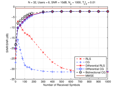
Figure 4: SINR performance comparison of proposed CG algorithms over a single path channel where all schemes have been trained with 150 symbols and then switched to decision directed mode.

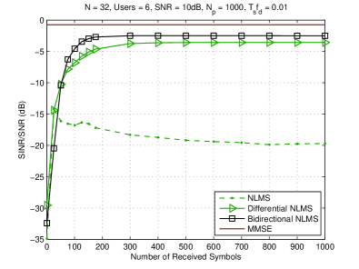
Figure 5: SINR performance comparison of proposed NLMS algorithms over a single path channel where all schemes have been trained with 150 symbols and then switched to decision directed mode.

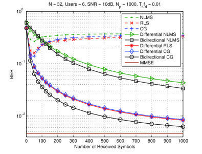
Figure 6: BER performance comparison of proposed schemes during training over a single path channel.

The BER performance of the differential and bidirectional schemes is illustrated in Fig. 6, where the system parameters are equal to those of Figs. 4 and 5. The RLS and CG algorithms converge to near the MMSE level with the bidirectional scheme providing a performance improvement over other considered algorithms. The NLMS schemes exhibit slower BER convergence compared to their SINR performance but reach a level where decision directed operation can take place in a severely fading channel. Due to the superior performance of the CG and RLS based algorithms we predominantly focus on their performance for the remainder of this section.

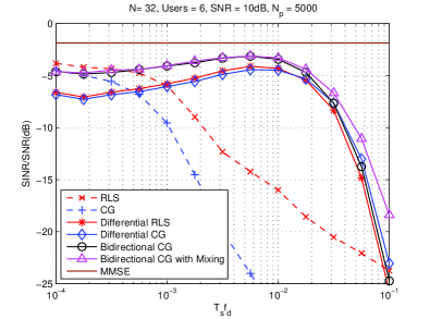
Figure 7: SINR performance versus fading rate of the proposed CG schemes over a single path channel after 200 training symbols.

Fig. 7 illustrates the performance of the proposed CG and RLS algorithms as the fading rate is increased. The conventional schemes with RLS and CG algorithms are unable to cope with fading rates in excess of $T_{s}f_{d}=0.005$ and begin to diverge at the completion of the training sequence. The proposed bidirectional scheme outperforms the differential schemes but the performance begins to decline once fading rates above $f_{d}T_{s}=0.01$ are reached. Once again, the increase in performance of the bidirectional scheme can be accounted for by the increased correlation information supplied by the matrices $\mathbf{F}_{2}$ and $\mathbf{F}_{3}$ and data reuse. The introduction of the mixing factors into the bidirectional algorithm improves performance further, especially at higher fading rates. A first reason for this is the improvement in consistency as previously mentioned. However, a second more significant reason can be established by referring back to the observations on the correlation factors $f_{1-3}$. Although fading rates of $0.01$ may be fast, the assumption $h[i-2]\approx h[i-1]\approx h[i]$ is still valid. Consequently, $f_{1}\approx f_{2}\approx f_{3}$ and equal weighting is adequate. However, as the fading rate increases beyond $T_{s}f_{d}=0.01$ this assumption breaks down and the correlation information requires unequal weighting for optimum performance, a task fulfilled by the adaptive mixing factor.

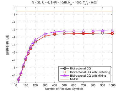
Figure 8: SINR performance over a single path channel of the proposed schemes with switching and mixing factors.

A more detailed plot illustrating the performance advantages of the CG switching and mixing parameters presented in is given by Fig. 8. The switching approach provides little improvement over the standard bidirectional scheme due to its discrete and non-adaptive operation. As previously covered, a low instantaneous value of $f_{1-3}$, as indicated by a large power differential, does not indicate that all information gathered on $f_{1-3}$ is redundant. The mixing parameter implementations address this shortcoming by adaptively setting the parameters via the error weight expression (21) that accurately reflects the averaged correlation factors. At a fading rate of $T_{s}f_{d}=0.02$ the assumption of $f_{1}\approx f_{2}\approx f_{3}$ begins to diminish in accuracy and therefore unequal weighting is required for performance in excess of the standard bidirectional scheme, as previously mentioned and shown in Fig. 8.

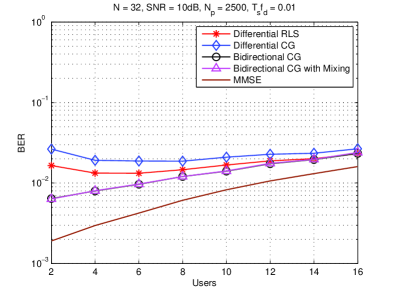
Figure 9: BER performance against system loading after 500 symbols of the proposed schemes over a single path channel. Schemes are trained with 150 symbols and then switch to decision directed operation.

The MUI suppression of the proposed and existing schemes is given by Fig. 9. The bidirectional scheme has significantly improved multiuser performance compared to the differential algorithms at low system loads but diminishes as the number of users increases. This behavior supports the analytical conclusions of Section VI-A by virtue of the convergence of the differential and bidirectional schemes and the increasing accuracy of (63) as system loading, and therefore received power, increases.

VII-B Cooperative DS-CDMA

To further demonstrate the performance of the proposed schemes in cooperative relaying systems [5], we apply them to an AF cooperative DS-CDMA system detailed in Section II.

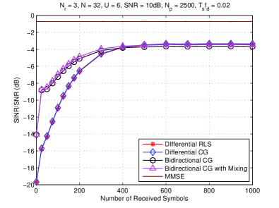
Figure 10: SINR performance of the proposed CG schemes during training in a single path cooperative DS-CDMA system.

Fig. 10 shows that the bidirectional scheme obtains performance benefits over the differential schemes during convergence but, as expected, the performance gap closes as steady-sate is reached. The inclusion of variable mixing parameters improves performance but to a lesser extent than non-cooperative networks due to the more challenging scenario of compounding highly time-variant channels.

Figure 11: BER performance of the proposed CG schemes in a single path cooperative DS-CDMA system.

The improvement BER brought about by the bidirectional schemes is evident from Figure 11. However, the more challenging environment of a cooperative system with compounded rapid fading has impacted on the BER performance of the schemes, as evidenced by the increased performance gap between the proposed schemes and MMSE reception.

VIII Conclusions

In this paper, we have presented a bidirectional MMSE framework that exploits the correlation characteristics of rapidly varying fading channels to overcome the problems associated with conventional adaptive interference suppression techniques in such channels. An analysis of the proposed schemes has been performed and the reasons behind the performance improvements shown to be the additional correlation information, data reuse and optimised correlation factor weighting. The conditions under which the differential and bidirectional schemes are equivalent have also been established and the steady-state implications of this detailed. Finally, the proposed algorithms have been assessed in standard and cooperative multiuser DS-CDMA systems and shown to outperform both differential and conventional schemes.

References

- [1] S. Verdu, Multiuser Detection. Cambridge University Press, NY, 1998.
- [2] U. Madhow and M. Honig, “MMSE interference suppression for direct-sequence spread spectrum CDMA,” IEEE Transactions on Communications, vol. 42, no. 12, pp. 3178–3188, December 1994.
- [3] W. Huang, Y. Wong, and C. Kuo, “Decode-and-forward cooperative relay with multi-user detection in uplink CDMA networks,” in IEEE Global Telecoms. Conf., Pheonix, November 2007.
- [4] R. C. de Lamare, “Joint iterative power allocation and linear interference suppression algorithms for cooperative ds-cdma networks,” IET Communications, vol. 6, no. 13, pp. 1930–1942, Sept 2012.
- [5] P. Clarke and R. C. de Lamare, “Transmit diversity and relay selection algorithms for multirelay cooperative mimo systems,” IEEE Transactions on Vehicular Technology, vol. 61, no. 3, pp. 1084–1098, March 2012.
- [6] T. Wang, R. C. de Lamare, and P. D. Mitchell, “Low-complexity set-membership channel estimation for cooperative wireless sensor networks,” IEEE Transactions on Vehicular Technology, vol. 60, no. 6, pp. 2594–2607, July 2011.
- [7] T. Wang, R. C. de Lamare, and A. Schmeink, “Joint linear receiver design and power allocation using alternating optimization algorithms for wireless sensor networks,” IEEE Transactions on Vehicular Technology, vol. 61, no. 9, pp. 4129–4141, Nov 2012.
- [8] T. Peng, R. C. de Lamare, and A. Schmeink, “Adaptive distributed space-time coding based on adjustable code matrices for cooperative mimo relaying systems,” IEEE Transactions on Communications, vol. 61, no. 7, pp. 2692–2703, July 2013.
- [9] R. C. de Lamare, R. Sampaio-Neto, and A. Hjorungnes, “Joint iterative interference cancellation and parameter estimation for cdma systems,” IEEE Communications Letters, vol. 11, no. 12, pp. 916–918, December 2007.
- [10] R. C. de Lamare and R. Sampaio-Neto, “Minimum mean squared error iterative successive parallel arbitrated decision feedback detectors for DS-CDMA systems,” IEEE Trans. Commun., vol. 5, no. 56, pp. 778–789, May 2008.
- [11] R. C. de Lamare, “Adaptive and iterative multi-branch mmse decision feedback detection algorithms for multi-antenna systems,” IEEE Transactions on Wireless Communications, vol. 12, no. 10, pp. 5294–5308, October 2013.
- [12] R. de Lamare and P. Diniz, “Set-membership adaptive algorithms based on time-varying error bounds for cdma interference suppression,” IEEE Transactions on Vehicular Technology, vol. 58, no. 2, pp. 644–654, Feb 2009.
- [13] S. Haykin, Adaptive Filter Theory, 4th ed. NJ: Prentice Hall, 2002.
- [14] D. Sadler and A. Manikas, “MMSE multiuser detection for array multicarrier DS-CDMA in fading channels,” IEEE Trans. Signal Process., vol. 53, no. 7, pp. 2348–2358, July 2005.
- [15] R. Schoder, W. Gerstacker, and A. Lampe, “Noncoherent MMSE interference suppression for DS-CDMA,” IEEE Trans. Commun., vol. 50, no. 4, pp. 577–587, April 2002.
- [16] S. Haykin, A. Sayed, J. Zeidler, P. Yee, and P. Wei, “Adaptive tracking of linear time variant systems by extended RLS algorithms,” IEEE Trans. Signal Process., vol. 45, no. 5, pp. 1118–1128, May 1997.
- [17] J. Wang, “Fast tracking RLS algorithm using novel variable forgetting factor with unity zone,” IEEE Electronics Letters, vol. 27, no. 23, pp. 2550–2551, November 1991.
- [18] R. Kwong and E. Johnston, “A variable step size LMS algorithm,” IEEE Trans. Signal Process., vol. 40, no. 7, pp. 1633–1642, May 1992.
- [19] B. Toplis and S. Pasupathy, “Tracking improvements in fast RLS algorithm using a variable forgetting factor,” IEEE Trans. Acoust., Speech, Signal Process., vol. 36, no. 2, pp. 206–227, February 1988.
- [20] S.-H. Leung and C. So, “Gradient-based variable forgetting factor RLS algorithm in time-varying environments,” IEEE Trans. Signal Process., vol. 53, no. 8, pp. 3141–3150, August 2005.
- [21] S. Hyun-Chool, A. Sayed, and S. Woo-Jin, “Variable step-size NLMS and affine projection algorithms,” IEEE Signal Process. Letters, vol. 11, no. 2, pp. 132–135, February 2004.
- [22] Y. Zhang, N. Li, J. Chambers, and Y. Hao, “New gradient-based variable step size LMS algorithms,” EURASIP Journal on Adv. in Signal Process., January 2008.
- [23] S. Gelfand, Y. Wei, and J. Krogmeier, “The stability of variable step-size LMS algorithms,” IEEE Trans. Signal Process., vol. 47, no. 12, pp. 3277–3288, December 1999.
- [24] P. Baracca, S. Tomasin, L. Vangelista, N. Benvenuto, and A. Morello, “Per sub-block equalization of very long ofdm blocks in mobile communications,” IEEE Transactions on Communications, vol. 59, no. 2, pp. 363–368, February 2011.
- [25] S. Yerramalli, M. Stojanovic, and U. Mitra, “Partial fft demodulation: A detection method for highly doppler distorted ofdm systems,” IEEE Transactions on Signal Processing, vol. 60, no. 11, pp. 5906–5918, Nov 2012.
- [26] L. Li, A. Burr, and R. de Lamare, “Joint iterative receiver design and multi-segmental channel estimation for ofdm systems over rapidly time-varying channels,” in IEEE 77th Vehicular Technology Conference (VTC Spring) 2013, June 2013, pp. 1–5.
- [27] Y. Cai, R. C. de Lamare, and R. Fa, “Switched interleaving techniques with limited feedback for interference mitigation in ds-cdma systems,” IEEE Transactions on Communications, vol. 59, no. 7, pp. 1946–1956, July 2011.
- [28] M. L. Honig and J. S. Goldstein, “Adaptive reduced-rank interference suppression based on the multistage wiener filter,” IEEE Transactions on Communications, vol. 6, no. 50, pp. 986–994, June 2002.
- [29] Y. Sun, V. Tripathi, and M. L. Honig, “Adaptive, iterative, reducedrank (turbo) equalization,” IEEE Transactions on Wireless Communications, vol. 4, no. 6, pp. 2789–2800, March 2005.
- [30] R. C. de Lamare and R. Sampaio-Neto, “Reduced–rank adaptive filtering based on joint iterative optimization of adaptive filters,” IEEE Signal Process. Lett., vol. 14, no. 12, pp. 980–983, December 2007.
- [31] ——, “Reduced-rank space–time adaptive interference suppression with joint iterative least squares algorithms for spread-spectrum systems,” IEEE Transactions Vehicular Technology, vol. 59, no. 3, pp. 1217–1228, March 2010.
- [32] ——, “Adaptive reduced-rank equalization algorithms based on alternating optimization design techniques for MIMO systems,” IEEE Transactions on Vehicular Technology, vol. 60, no. 6, pp. 2482–2494, July 2011.
- [33] ——, “Adaptive reduced-rank processing based on joint and iterative interpolation, decimation, and filtering,” IEEE Transactions on Signal Processing, vol. 57, no. 7, pp. 2503–2514, July 2009.
- [34] S. Li, R. C. de Lamare, and R. Fa, “Reduced-rank linear interference suppression for ds-uwb systems based on switched approximations of adaptive basis functions,” IEEE Transactions on Vehicular Technology, vol. 60, no. 2, pp. 485–497, Feb 2011.
- [35] R. C. de Lamare, R. Sampaio-Neto, and M. Haardt, “Blind adaptive constrained constant-modulus reduced-rank interference suppression algorithms based on interpolation and switched decimation,” IEEE Transactions on Signal Processing, vol. 59, no. 2, pp. 681–695, Feb 2011.
- [36] M. Honig, M. Shensa, S. Miller, and L. Milstein, “Performance of adaptive linear interference suppression for DS-CDMA in the presence of flat rayleigh fading,” in IEEE Vehicular Technology Conf., Pheonix, May 1997.
- [37] H. V. Poor and X. Wang, “Adaptive multiuser detection in fading channels,” in Annual Allerton Conf. Commun., Control and Computing, Monticello, October 1996.
- [38] U. Madhow, K. Bruvold, and L. J. Zhu, “Differential MMSE: A framework for robust adaptive interference suppression for DS-CDMA over fading channels,” IEEE Trans. Commun., vol. 53, no. 8, pp. 1377–1390, August 2005.
- [39] L. J. Zhu and U. Madhow, “Adaptive interference suppression for direct sequence CDMA over severely time-varying channels,” in IEEE Global Telecoms. Conf., Pheonix, Novmeber 1997.
- [40] M. Honig, S. Miller, M. Shensa, and L. Milstein, “Performance of adaptive linear interference suppression in the presence of dynamic fading,” IEEE Trans. Commun., vol. 49, no. 4, pp. 635–645, April 2001.
- [41] P. S. R. Diniz, Adaptive Filtering: Algorithms and Practical Implementation, 3rd ed. Springer, August 2008.
- [42] C. Meyer, Matrix Analysis and Applied Linear Algebra. SIAM, February 2001.
- [43] D. G. Luenburger and Y. Ye, Linear and Nonlinear Programming, 3rd ed. Springer, 2008.
- [44] J. Lee, H. Yu, and Y. Sung, “Beam tracking for interference alignment in time-varying mimo interference channels: A conjugate-gradient-based approach,” IEEE Transactions on Vehicular Technology, vol. 63, no. 2, pp. 958–964, Feb 2014.
- [45] P. S. Chang and A. N. Wilson, “Analysis of conjugate gradient algorithms for adaptive filtering,” IEEE Trans. Signal Process., vol. 48, no. 2, pp. 409–418, February 2000.
- [46] N. J. Bershad, J. C. M. Bermudez, and J.-Y. Yourneret, “An affine combination of two LMS adaptive filters - transient mean square analysis,” IEEE Trans. Signal Process., vol. 56, no. 8, May 2008.
- [47] J. Arenas-Garcia, A. Figueiras-Vidal, and A. Sayed, “Mean-square performance of a convex combination of two adaptive filters,” IEEE Trans. Signal Process., vol. 45, no. 3, pp. 1078–1090, March 2006.
- [48] H. Kushner, Approximation and Weak Convergence Methods for Random Processes with Applications to Stochastic System Theory. MIT Press, April 1984.
- [49] A. Sayed, Adaptive Filters. John Wiley & Sons, May 2008.
- [50] W. Jakes, Microwave Mobile Communications. Wiley-IEE Press, May 1994.