No-go theorem for the description of Mott phenomena with conventional Density Functional Theory methods.

Abstract

Density functional theory provides the most widespread framework for the realistic description of the electronic structure of solids, but the description of strongly-correlated systems has remained so far elusive. Here we consider a particular limit of electrons in a periodic ionic potential in which a one-band description becomes exact all the way from the weakly-correlated metallic regime to the strongly-correlated Mott-Hubbard regime. We provide a necessary condition a density functional should fulfill to describe Mott-Hubbard behaviour and show that it is not satisfied by standard and widely used local, semilocal and hybrid functionals. We illustrate the condition in the case of a few-atom system and provide an analytic approximation to the exact exchange-correlation potential based on a variational wave function which shows explicitly the correct behaviour providing a robust scheme to combine lattice and continuum methods.

ISC-CNR and Dipartimento di Fisica, Università di Roma “La Sapienza”, Piazzale Aldo Moro 2, 00185 Roma, Italy.

Beijing Computational Science Research Center, Beijing 100084, China.

CNR-IOM, Istituto Officina dei Materiali, Cittadella Universitaria, Monserrato (CA) 09042, Italy

Center S3, CNR Institute of Nanoscience, Via Campi 213/A, 41125 Modena, Italy.

Department of Theoretical Chemistry and Amsterdam Center for Multiscale Modeling, FEW, Vrije Universiteit Amsterdam, Amsterdam 1081 HV, Netherlands.

Density functional theory (DFT) plays a fundamental role to understand matter around us[1], however it relies on approximations that fail to describe phenomena encountered in solids which have open d, or f shells such as Mott-Hubbard insulating behavior[2], and correlation-induced band narrowing close to the Mott phase[3] and in heavy-fermions[4]. It is commonly believed that these deficiencies “cannot be remedied by using more complicated exchange-correlation functionals in DFT” (see Ref. [5]). Instead, these effects have been successfully described by means of lattice models, such as the Hubbard model,[6, 7, 8] employing a series of techniques which have evolved into modern Dynamical Mean-Field theory (DMFT)[9]. This led to intense efforts to combine lattice and DFT methods[10, 5, 11, 12, 13, 15].

In this work, we study a particular limit of correlated electrons in a solid where a one-band description becomes exact. More precisely the continuum model of electrons in a periodic potential and a generalized one-band Hubbard model are bound to provide quantitatively equivalent solutions. In this limit we derive a necessary condition a functional should satisfy to be able to describe Mott-Hubbard behavior. We show that most functionals in use today in chemistry and physics, including local, semilocal and hybrid functionals,[14] do not satisfy the condition and they cannot describe Mott-Hubbard phenomena. This provides a rigorous ground to the quoted statement of Ref. [5] when restrained to conventional approximations. On the other hand, we also show that in simple test cases a suitable combination of DFT and lattice methods can produce an exchange-correlation (xc) potential, that not only shows the correct qualitative behavior, but it is also in surprisingly good agreement with results in test systems tractable with accurate wave-function methods.

1 Results

1.1 Continuum model and one-band limit

We consider a fictitious system consisting of $N$ electrons moving in the potential $v_{\rm ext}$ produced by a collection of $N$ identical nuclei of charge $Ze$ located on the sites ${\bf R}_{i}$ of a periodic lattice with spacing $a$. The system can be viewed as a half-filled 1s band in which $Z$ controls the orbital size, $a_{\rm B}/Z$, with $a_{\rm B}$ the Bohr radius. Using $a_{\rm B}/Z$ as the unit of length and $Z^{2}$Ha as the unit of energy the Hamiltonian reads,

$$H=\sum_{i}^{N}\hat{h}({\bf r}_{i})+\frac{1}{2Z}\sum_{i\neq j}^{N}\frac{1}{|{\bf r}_{i}-{\bf r}_{j}|}$$ (1)

where ${\bf r}_{i}$ are the electron coordinates and $\hat{h}({\bf r})$ is the one-body Hamiltonian, $\hat{h}({\bf r})=-\frac{1}{2}\nabla_{{\bf r}}^{2}+v_{\rm ext}({\bf r})$ with,

$$v_{\rm ext}({\bf r})=-\sum_{j}^{N}\frac{1}{|{\bf r}-{\bf R}_{j}|}.$$

Notice that, in these rescaled units, the one-body part becomes $Z$-independent and $1/Z$ plays the role of a coupling constant[16]. We will use $a$ and $Z$ as our control variables.

Our first goal is to find a region of the parameter space ($a,Z$), where a one-band (1B) lattice model describes quantitatively and not only qualitatively the continuum model defined by equation (1). As it is well known from studies of the Hubbard model,[6, 8, 7, 17, 18] the most important energy scales in this problem are the Hubbard on-site interaction, $U$, and the nearest-neighbor hopping matrix element, $t$, which define the weakly-correlated regime, $0<U\ll zt$, and the strongly-correlated regime, $U\gg zt$, $z$ denoting the lattice coordination.

In the atomic limit, for $Z=1$, the elimination of higher energy bands is inaccurate, since the energy cost[19] $U=0.47$ Ha of a charge fluctuation $1s^{1}1s^{1}\rightarrow 1s^{0}1s^{2}$ is similar to the cost $\Delta=3/8$ Ha of a charge fluctuation $1s^{1}1s^{1}\rightarrow 1s^{1}2s^{1}$. To avoid this problem we take the limit of large $Z$ adjusting $a\sim\log(Z)$ so that $t/U$ is kept constant (hereafter “the 1B limit”). In this limit the condition

$$\Delta\gg t,U,$$ (2)

is fulfilled allowing us to study quantitatively Mott-Hubbard phenomena in the model equation (1) from the weak to the strongly-correlated regime within a 1B description. Figure 1 shows how this works for the Hubbard repulsion. As $Z$ grows the “screened” $U$ asymptotically approaches the bare $U_{0}$ showing that corrections from higher orbitals become irrelevant.

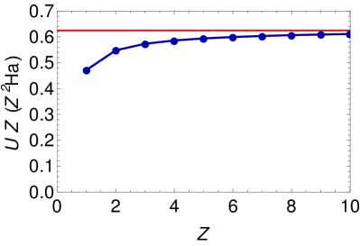
Figure 1: Vanishing of screening effects at large atomic number. The 1s Hubbard $U$ vs. the atomic number. We multiply $U$ by $Z$ so that the limiting value is a constant in our units. The red line is the bare value $U_{0}$ from Coulomb integrals [equation (15)], while the blue dots are the “screened” value obtained as $U=E_{I}^{Z,Z}-E_{I}^{Z,Z-1}$ where $E_{I}^{Z,N}$ is the $N$-th ionization energy for atomic number Z. ($E_{I}^{1,0}\equiv E_{A}$ is the affinity energy for Hydrogen)[19].

1.2 Lattice Model.

In the 1B limit the continuum model is equivalent to a generalized Hubbard model which can be obtained by the standard second-quantization procedure employing a single particle basis of 1s orbitals $\phi_{i}({\bf r})$ centered at ${\bf R}_{i}$ (see Methods and Refs. [6, 8, 7, 20, 21, 22]). It will become clear below that our arguments are sufficiently general that are valid for such generalized Hubbard model. However to fix ideas it is useful to think in terms of the standard Hubbard model[6, 8, 7] which can be obtained by absorbing the long-range part of the Coulomb interaction in mean-field in the on-site energy $v$ and restricting the hopping to nearest neighbors $\langle ij\rangle$,

$$H_{H}=\sum_{i\sigma}v\,n_{i\sigma}-t\sum_{\langle ij\rangle\sigma}(c_{i\sigma}^{{\dagger}}c_{j\sigma}+{\rm H.c.})+U\sum_{i}n_{i\uparrow}n_{i\downarrow},$$ (3)

with $c_{i\sigma}$ ( $c^{{\dagger}}_{i\sigma}$) the annihilation (creation) operator for an electron with spin $\sigma$ on site $i$ and $n_{i\sigma}\equiv c^{{\dagger}}_{i\sigma}c_{i\sigma}$.

To link lattice and DFT descriptions, we need the correlated density which is determined by the one-body density matrix of the lattice model ($\rho_{ij}\equiv\sum_{\sigma}\langle c_{j\sigma}^{\dagger}c_{i\sigma}\rangle$) and the $\phi_{i}$’s (Methods). The density can be separated into an “atomic” component and a “bond-charge” contribution, $n({\bf r})=n_{\rm at}({\bf r})+n_{\rm bd}({\bf r})$ with,

$$n_{\rm at}({\bf r}) = \sum_{i}|\phi_{i}({\bf r})|^{2}\rho_{ii}$$ (4)

$$n_{\rm bd}({\bf r}) = \sum_{\langle ij\rangle}\phi_{j}^{*}({\bf r})\phi_{i}({\bf r})\rho_{ab}+c.c.,$$ (5)

where, we used the fact that for large $a$ the sums in equation (5) can be restricted to nearest-neighbors and we defined the nearest-neighbor density-matrix element $\rho_{ij}=\rho_{ab}$. In our case, $\rho_{ii}=1$, thus all the dependence of the density on $U/t$ is encoded in the bond charge and it is controlled by $\rho_{ab}$. In the limit of large $Z$, we can study the system from small to large $U/t$ either varying $a$ or changing $Z$ at a fixed $a$. In the latter case, since the $\phi_{j}$’s can be taken as fixed independently of the value of $U/t$, equation (5) establishes a one to one mapping between the density and $\rho_{ab}$ as $U/t$ (or equivalently $Z$) is varied.

1.3 Hartree approximation

Before examining DFT, we analyze the ground state of Hamiltonian equation (1) in the Hartree approximation. As an initial guess of the Hartree orbitals, we can take the eigenstates of the non-interacting problem. We will show below that the Hartree potential $v_{H}({\bf r})$ is of order $O(1/Z)$, thus, since $\Delta$ is $O(Z^{0})$, the corrections to the initial guess can be neglected and, to leading order in $1/Z$, the Hartree orbitals coincide with the non-interacting orbitals and the Hartree self-consistent density coincides with the non-interacting density. To fix ideas consider the case $N=2$, although the arguments are easily generalized to any $N$. The initial guess of the occupied Hartree orbital is the bonding state,

$$\psi_{0}^{\rm H}({\bf r})=\frac{1}{\sqrt{2}}[\phi_{a}({\bf r})+\phi_{b}({\bf r})].$$

Here $i=a,b$ labels the two ions and we assume real orbitals. The Hartree density $n^{H}({\bf r})$ is given by $n^{H}({\bf r})=2|\psi_{0}^{\rm H}({\bf r})|^{2}$ or equivalently by eqs. (4),(5) inserting $\rho_{ij}$ in the Hartree approximation, $\rho_{ij}^{H}$, where for two-sites $\rho_{ab}^{H}=1$.

The Hartree potential is given by,

$$v_{H}({\bf r})=\frac{1}{Z}\int d^{3}{\bf r}^{\prime}\frac{n^{H}({\bf r}^{\prime})}{|{\bf r}-{\bf r}^{\prime}|}.$$

This is finite everywhere and it has a maximum that scales at most as $1/Z$. Thus, we can always choose $Z$ large enough so that $v_{H}/\Delta\sim 1/Z$ is small and the non-interacting orbitals coincide with the Hartree orbitals.

1.4 How Mott-Hubbard correlations are encoded in the density

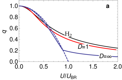
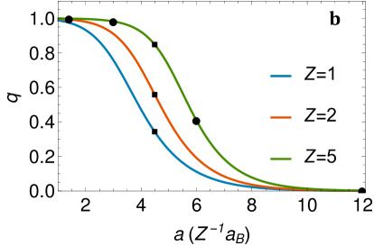
Figure 2: Hopping reduction factor. a Exact results (full lines) as a function of $U/U_{\rm BR}$ for the Hubbard model in dimension $D$. Here $U_{\rm BR}$ is a measure of the effective non-interacting bandwidth[23], $U_{\rm BR}\equiv\frac{16}{N}\sum_{k\in{\rm occ.}}\epsilon_{k}$ where $\epsilon_{k}$ are the single particle non-interacting energies and the sum is restricted to the occupied states. We show results for a two-site system (black), for an infinite chain (red) and for the Bethe lattice in infinite dimensions (blue). The Bethe lattice data where derived from numerical[24] and analytic[25] results (full blue line). The cusp signals $U_{\rm c2}$ where the Mott-Hubbard transition occurs from the metallic phase ($U<U_{\rm c2}$) to the insulating phase ($U>U_{\rm c2}$). The dashed line was obtained with the Gutzwiller wave function for the same Bethe lattice. b Hopping reduction factor obtained with a Gutzwiller type wave function in an hydrogenic molecule as a function of atom separation $a$ for different atomic numbers. The dots (squares) correspond to the cases considered in Fig. 4 (Fig. 3 and Supplementary Fig. S1).

Since DFT provides an exact description[1], Mott-Hubbard behavior should be encoded in the density. In the present limit this can only happen through the bond charge equation (5) which can be parametrized through the hopping reduction factor defined as,

$$q\equiv\frac{\rho_{ab}}{\rho_{ab}^{H}}.$$

For an interacting system, one typically finds $q<1$. For example Fig. 2a shows the hopping reduction factor of the Hubbard model for exactly solvable lattices. In more general cases, a good estimate of the hopping reduction factor can be obtained with a variational Gutzwiller wave function (see Suppplementary Note 1). For the two-site Hubbard model, this yields the exact solution while for infinite dimension it provides an accurate estimate in the metallic phase (dashed line in Fig. 2).

For the full model equation (14), the qualitative behavior of the hopping reduction factor does not change as it can be easily checked using perturbation theory. Fig. 2b shows the hopping reduction factor computed with a variational Gutzwiller-type wave function for the two-site full model (Methods) as a function of the interatomic distance, $a$. Since $t$ decreases exponentially with $a$ one obtains a rapid crossover from the weakly-correlated regime ($q\sim 1$) to the strongly-correlated regime ($q\sim 0$). It is believed that the crossover turns into the Mott metal-insulator transition in high dimensional lattices as Fig. 2a suggests.

From the above discussion it is clear that in the 1B limit, independently of the dimensionality, the correlated charge in the bond is depleted with respect to a Hartree computation (c.f. equation (5) and Fig. 2). Figure 3 shows an accurate computation of the density within the full configuration interaction (CI) approach. For small $Z$ (strong correlation) the bond charge is indeed depressed, however, the differences are minute which makes extremely challenging for DFT to be sensitive to Mott-Hubbard correlations.

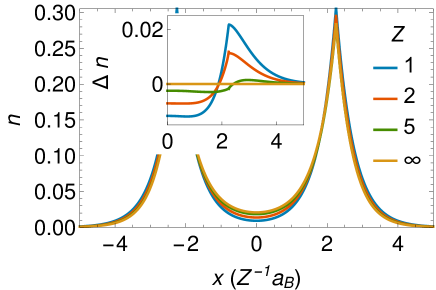
Figure 3: Charge along the bond for interatomic distance $a=4.5\ a_{B}Z^{-1}$ and various values of $Z$. The inset shows the interacting charge minus the nointeracting charge ($Z=\infty$). Charges where computed within full CI (see Methods).

1.5 No-go theorem.

In Kohn-Sham (KS) theory[26] the interacting system is mapped into a system of non-interacting electrons moving in an effective potential which is the sum of the external potential, the Hartree (H) potential and the xc-potential,

$$v_{\rm KS}({\bf r})=v_{\rm ext}({\bf r})+v_{\rm H}({\bf r})+v_{\rm xc}({\bf r}).$$ (6)

In the exact formulation the non-interacting system reproduces the exact density of the interacting system, however in practice $v_{\rm xc}$ is an unknown functional of the density and approximations are needed. In the local density approximation[26, 14] (LDA), the xc-potential is a simple function of the local density, $v^{\rm LDA}_{\rm xc}({\bf r})=v_{\rm xc}^{\rm LDA}[n({\bf r})]$. We show now that LDA cannot account for Mott-Hubbard correlations of the system.

To solve KS equations in LDA one can use again the Hartree density, $n^{H}$, as a starting guess. Using a standard parametrization of the potential, it is easy to show that $v^{\rm LDA}_{\rm Hxc}$ is at most of order $\sim 1/Z$ (see Suppplementary Note 2). For large $Z$, the change in the orbitals is then of order $v_{\rm xc}^{\rm LDA}/\Delta\sim 1/Z$ and it can be neglected. Thus in the 1B limit LDA orbitals coincide with the Hartree orbitals and the density is given by equations (4), (5) with $\rho_{ij}^{\rm LDA}=\rho_{ij}^{H}$ independently of $U/t$. It is clear that LDA cannot account for the bond-charge reduction which is a primary characteristic of Mott-Hubbard correlations.

The failure of LDA can be traced back to the $1/Z$ scaling of $v_{\rm xc}$. Clearly, the exact $v_{\rm xc}$ cannot scale as $1/Z$ everywhere, since if it did so, the same argument as for LDA would apply. The only way to generate the correlated density with a non-interacting system is by modifying the orbitals, and this can only happen by allowing the low-energy 1s states to be mixed with high energy single particle states outside the minimal basis set, consistently with the known fact that exact KS-DFT breaks down when restricted to a finite basis set.[27, 28]

For large $Z$ the mixing of the 1s band with the higher bands can only be achieved if the xc-potential is of order $Z^{0}$. It follows that a necessary condition that a functional must satisfy to describe Mott-Hubbard behavior in the limit in which the 1B mapping is accurate is that the potential should have regions which scale as $Z^{0}$. Any functional whose xc-potential scales to zero when $Z\rightarrow\infty$ (keeping $U/t$ constant) cannot describe Mott-Hubbard behavior. This is the case for local semilocal and hybrid functionals[29] (see Suppplementary Note 2). and even the exact DFT strongly-correlated limit[30, 31], which uses a wavefunction with maximally correlated electrons to compute the expectation of the electron-electron interaction, and becomes exact in the limit $a\gg Z$, but not in the present case, $a\sim\log(Z)$.

1.6 Mott barriers

How does the exact xc-potential look like? It should have a barrier in the bond to deplete the KS density, a well-known result from the study of molecules.[32, 33, 34, 35, 36] We term the part of the xc-potential that scales as $Z^{0}$ a “Mott barrier”. It can be proved that the barrier height in the strongly-correlated regime is related to the ionization potential of the system;[32, 33, 34, 35, 36] it is therefore of order $O(Z^{0})$ as expected from the previous arguments.

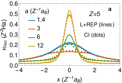
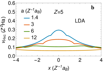
Figure 4: Hartree-exchange-correlation potential for a two-site system. The potential is plotted along the bond direction $x$ for $z=y=0$, $Z=5$ and different values of the interatomic distance $a$. The dots in a are obtained inverting the full CI density while panel b shows the LDA. [37] The lines in a are the L+REP approximation using orthogonalized atomic orbitals. The strength of the correlations for each case is defined by the value of $q$ in Fig. 2.

To illustrate the Mott-barrier effect and develop an approximation for the exact potential, we follow a long tradition[2, 38] and study a two-site system as a proxy for the lattice. As in the pioneering works of Refs. [32, 33, 34, 35, 36] we compute the Hxc-potential, $v_{\rm Hxc}\equiv v_{\rm H}+v_{\rm xc}$, by inverting Kohn-Sham equations with the full CI densities as an input (Methods). In Figure 4 we compare the CI xc-potential (dots in panel a) with the LDA (panel b). We see that for large $a$ (strong-correlation) a large barrier develops in the bond while this effect is missed by the LDA.

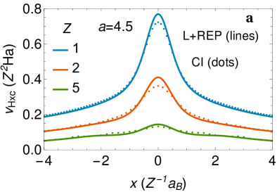
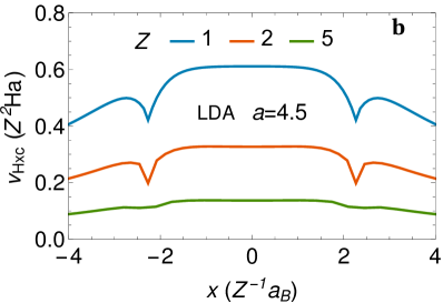
Figure S1: Mott Barrier vs. $Z$. Hartree exchange-correlation potential for $a=4.5Z^{-1}a_{B}$ and different values of $Z$ for the two-site system as a function of $x$ for $z=y=0$ obtained inverting the full CI ground state density as explained in Methods (dots in a) and in the LDA[37] (b). The lines in a are analytic expressions based on the L+REP approximation. The strength of the correlations for each case is defined by the value of $q$ in Fig. 2.

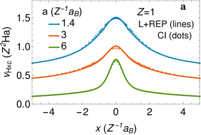
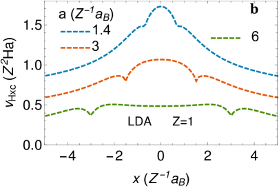
Figure S2: Hartree-exchange-correlation potential for the stretched Hydrogen molecule. We show $v_{\rm Hxc}$ as a function of $x$ for $z=y=0$ for different values of $R$. The dots in a where obtained inverting the full CI ground state density as explained in Methods while the lines are the L+REP results. Panel b shows the LDA results. The cases $a=1.4$ and $a=3$ where shifted by 0.5 and 0.25 respectively ($Z^{2}$Ha) for clarity. The first two cases are in the weakly and intermediate correlation regimes while the case $a=6$ is in the strong coupling regime (c.f. Figs. 2b and 5b).

Supplementary Figures S1 and S2 show that the arguments developed rigorously for large $Z$ still describe the behavior for fixed $a$ reducing $Z$, or for $Z=1$ changing $a$. Notice, however that for the latter (Fig. S2) the barrier becomes smaller as one goes to larger $a$ which may seem surprising according to our previous arguments. Also in all weakly-correlated cases (Fig. 4 and Supplementary Figures S1 and S2) a broad small barrier appears and LDA performs reasonably well. This barrier is of a different physical origin as discussed below.

The solid lines in Figs. 4a (see also Supplementary Figures S1a and S2a) represent a reverse-engineering potential (REP) obtained from an approximate analytical inversion of KS equations combined with the solution of the lattice problem (L+REP) constructed from orthogonalized 1s atomic orbitals (Methods). This inversion, involving a Laplacian, is a singular task so that subtle errors in the density propagate to give large errors in the potential and the task may seem hopeless with such a rough basis. Since a large source of error comes from the basis, we first derive equations to optimize it (Methods and Refs. [21, 22]). Fortunately, the solution of these equations is not needed. Instead, one finds that they can be used to eliminate the Laplacian, yielding equations which are much less sensitive to the basis and can be evaluated with approximate orbitals (see Suppplementary Note 3). The resulting expressions for the Hartree-exchange-correlation potential read,

$$v_{\rm Hxc}({\bf r})=v_{\rm xc}^{{\rm kin}}({\bf r})+v_{\rm xc}^{{\rm resp}}({\bf r})+v_{\rm Hxc}^{{\rm cond}}({\bf r})$$ (7)

with

$$v_{\rm xc}^{{\rm kin}}({\bf r}) = \frac{(1-q^{2})}{2}\frac{|\phi_{a}({\bf r})\vec{\nabla}\phi_{b}({\bf r})-\phi_{b}({\bf r})\vec{\nabla}\phi_{a}({\bf r})|^{2}}{n^{2}({\bf r})}$$ (8)

$$v_{\rm xc}^{{\rm resp}}({\bf r}) = \frac{t(1-q)[\phi_{a}({\bf r})-\phi_{b}({\bf r})]^{2}}{n({\bf r})}+\delta\epsilon_{g}$$ (9)

$$v_{\rm Hxc}^{{\rm cond}}({\bf r}) = \frac{1}{Z}\int\frac{n_{2}({\bf r},{\bf r}^{\prime})}{n({\bf r})|{\bf r}-{\bf r}^{\prime}|}d{\bf r}^{\prime}.$$ (10)

where $\delta\epsilon_{g}>0$ is a small positive constant and $n_{2}({\bf r},{\bf r}^{\prime})$ is the two-body density[39]. The terms correspond one by one to the partition of the xc-potential obtained by Buijse et al. [39]. The present expressions, however, in terms of the lattice hopping reduction factor $q$ are new.

As shown in Fig. 4 and Supplementary Figures S1 and S2, using L+REP eqs. (8)- (10) yields a very accurate xc-potential from the weakly to the strongly-correlated regime. This holds even in the case $Z=1$ where the influence of higher energy orbitals could have spoiled the agreement (Supplementary Figures S1 and S2).

The first two terms in equation (7) are order $Z^{0}$ while the last term is at most of order $1/Z$ thus these equations show explicitly that the $v_{\rm xc}$ has parts with anomalous coupling constant scaling. Specifically the first term, which vanishes in the weakly-correlated limit ($q=1$), yields the Mott barrier.

In the large $Z$ limit and for large $a$ the above equations become particularly simple for the barrier height. Subtracting a small spurious constant term, there is no contribution from $v_{\rm xc}^{{\rm resp}}$ and the height separates in two contributions, one of Mott-Hubbard type and one of Coulomb form with different $Z$-scaling,

$$v_{\rm xc}^{{\rm kin}}(0) \simeq \frac{(1-q)}{2(1+q)}$$ (11)

$$v_{\rm Hxc}^{{\rm cond}}(0) \simeq \frac{1}{Za}.$$ (12)

Fig. 5a shows the barrier height as a function of $a$ for different $Z$. The dots are the numerical data while the full lines are obtained from equations (53)-(54) of Methods. Fig. 5b shows the barrier separated in the two components. LDA yields a quite good account of the $Z^{-1}$ component while the $Z^{0}$ component is completely missed. One can also see that the $Z^{0}$ component just reflects the $q$ behavior as a function of distance shown in Fig. 2. For Hydrogen, an accidental compensation of the distance dependence of the two components explains why the crossover was not identified in the potential before.

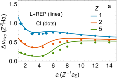
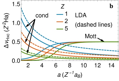
Figure 5: Barrier height. Height of the Hartree exchange-correlation potential at the bond midpoint for the two-site system as a function of internuclear separation for different $Z$. In a full lines are obtained using the L+REP approximation subtracting a small spurious term at infinity (equations (53)-(54) of Methods). Dots are obtained inverting the full CI charges. For $Z=1$, we include also data obtained with an accurate variational wave function (Methods). Diamonds are from Ref. [39]. b Shows separately the anomalously scaling Mott barrier height contribution, equation (53) and the contribution scaling as $1/(Za)$ (cond) from equation (54). The dashed lines are the LDA results.

1.7 Generalization to many atoms

To illustrate the relevance of these results for extended systems, we introduce a simple generalization of the L+REP equations (8)-(10) to the many-atom many-electron case. Equation (10) can be used without modification. Equations (8), (9) are important only in the strong correlation regime. In this case, since electrons are localized, we expect that the wave function resembles the two-site wave function. Thus eqs. (8), (9) are generalized by replacing the site labels $a$ and $b$ by site index $i$ and $j$ and summing over all $\langle i,j\rangle$ nearest-neighbor sites. $q$ is obtained from the solution of the lattice problem in the geometry considered.

Figure 3a shows the barriers for a four site H chain while b compares a quantum chemistry computation of the charge with the KS charge corresponding to the L+REP. The small difference between the two charges indicates that the L+REP is accurate also in this case.

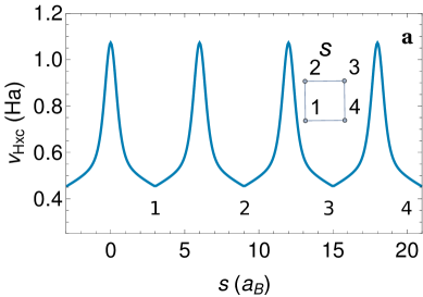
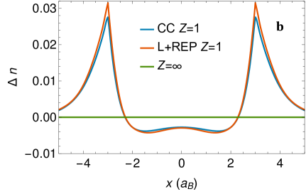
Figure 6: Mott barriers for a four atom chain. Panel a shows $v_{\rm Hxc}$ along the path shown in the inset for 4 H atoms arranged in a square with interatomic distance $a=6\ a_{B}$. Panel b compares the interacting charge computed with an accurate quantum chemistry method (CC) and the charge from the solution of the Kohn-Sham potential obtained with the L+REP method. Both are displayed as the difference between the interacting and the non-interacting charge ($Z=\infty$).

2 Discussion

It is often assumed that Kohn-Sham DFT bands do not show any renormalization due to interactions. Our results clearly indicate that the exact Kohn-Sham DFT bands will show band narrowing due to a suppression of tunneling stemming from Mott barriers (c.f. Fig. 4a, 6a, S1a and S2a). However, we have also shown that as soon as any conventional local semilocal, or hybrid functional is used, this effect is lost. Thus, although the assumption is in principle incorrect, in most practical computations available at present it is correct because the Mott barrier effect is not included.

The bond charge problem studied here provides different insight with respect to the fractional charge and fractional spin analysis[40], which correspond to the very stretched limit. Here we analyze explicitly a less extreme case, gaining important information on the more challenging intermediate correlation regime.

We find that the xc-potential separates naturally into two components, one with a conventional coupling constant scaling ($1/Z$) and one with an anomalous coupling constant scaling $Z^{0}$. Standard functionals capture only the first component, thus, those approaches in which Mott-Hubbard correlations are incorporated at a second stage modifying the conventional DFT band structure through DMFT or Gutzwiller approximations can be seen as a way to take into account the missing component.[5, 11, 12, 13, 15] We hope our results would allow to reformulate this approach in a more rigorous way to avoid double counting problems.

Clearly to obtain the anomalous coupling constant scaling directly from a functional is a highly non-trivial task. The present L+REP approach is a shortcut to this problem. In particular equation (8) establishes an intimate relationship between the suppression of tunneling in the lattice model and in the Kohn-Sham description linking in a neat way the two worlds of lattice models and DFT in the continuum.

Methods

2.1 Lattice Model.

The 1B model is obtained by expanding the field operators $\psi_{\sigma}({\bf r})$ and $\psi^{\dagger}_{\sigma}({\bf r})$ in a minimal basis consisting of $N$ Wannier orbitals $\phi_{i}({\bf r})\equiv\langle{\bf r}|i\rangle$ centered on the $N$ sites of the lattice,

$$\psi_{\sigma}({\bf r})=\sum_{i\sigma}\phi_{i}({\bf r})c_{i\sigma}+...\qquad{\rm and}\qquad\psi^{\dagger}_{\sigma}({\bf r})=\sum_{i\sigma}\phi^{*}_{i}({\bf r})c^{\dagger}_{i\sigma}+...$$ (13)

where the ellipsis indicate neglected higher energy states. For the scaling arguments it is enough to define $\phi_{i}({\bf r})$ as Wannier orbitals obtained from the lower band of Bloch states that diagonalize the non-interacting Hamiltonian (non-interacting Wannier orbitals). In the 1B limit defined in the main article they are very similar to orthogonalized atomic 1s orbitals. More accurate Wannier orbitals are discussed below.

Using eqs. (13), the 1B generalized Hubbard Hamiltonian corresponding to the continuum model defined in eq. (1) can be cast as

$$H_{\rm 1B}=H_{h}+H_{w}=\sum_{ij\sigma}h_{ij}c_{i\sigma}^{{\dagger}}c_{j\sigma}+\frac{1}{2}\sum_{ijkl\sigma\sigma^{\prime}}w_{ij,kl}c_{k\sigma}^{{\dagger}}c_{i\sigma^{\prime}}^{{\dagger}}c_{j\sigma^{\prime}}c_{l\sigma}$$ (14)

with $h_{ij}=\langle\ i|\hat{h}|j\rangle$ and

$$w_{ij,kl}=\int d^{3}{\bf r}d^{3}{\bf r}^{\prime}\phi_{k}^{*}({\bf r})\phi_{i}^{*}({\bf r}^{\prime})w({\bf r},{\bf r^{\prime}})\phi_{j}({\bf r}^{\prime})\phi_{l}({\bf r}),$$ (15)

with $w({\bf r},{\bf r^{\prime}})$ denoting Coulomb interaction:

$$w({\bf r},{\bf r^{\prime}})=\frac{1}{Z|{\bf r}-{\bf r}^{\prime}|}.$$ (16)

$H_{\rm 1B}$ is written in terms of bare matrix elements as, for example, the onsite Coulomb interaction $U_{0}\equiv w_{ii,ii}$. The effect of orbitals outside the basis is often accounted for[5] by replacing the bare matrix elements by screened matrix elements. However in the 1B limit this effect can be neglected and we drop the not (i.e. $U_{0}=U$).

Equations (13) can be also employed to relate the one- and two-particle densities, respectively $n({\bf r})$ and $n_{2}({\bf r},{\bf r}^{\prime})$ to the one and two-particle lattice density matrices as follows:

$$n({\bf r})=\sum_{\sigma}\langle\psi_{\sigma}^{\dagger}({\bf r})\psi_{\sigma}({\bf r})\rangle=\sum_{ij}\phi^{*}_{j}({\bf r})\phi_{i}({\bf r})\rho_{ij}.$$ (17)

and

$$n_{2}({\bf r},{\bf r^{\prime}})=\sum_{\sigma\sigma^{\prime}}\langle\psi_{\sigma^{\prime}}^{\dagger}({\bf r}^{\prime})\psi_{\sigma}^{\dagger}({\bf r})\psi_{\sigma}({\bf r})\psi_{\sigma^{\prime}}({\bf r}^{\prime})\rangle=\sum_{ijkl}\phi^{*}_{i}({\bf r})\phi_{j}({\bf r})\phi^{*}_{k}({\bf r}^{\prime})\phi_{l}({\bf r}^{\prime})D_{ij,kl}.$$ (18)

where we defined the spin-integrated two-body lattice density matrix, $D_{ij,kl}=\sum_{\sigma\sigma^{\prime}}\langle c_{i\sigma}^{{\dagger}}c_{k\sigma^{\prime}}^{{\dagger}}c_{l\sigma^{\prime}}c_{j\sigma}\rangle$. The density of the Hartree state is recovered by inserting in eq. (17) the Hartree lattice density matrix, $\rho_{ij}^{H}$, i.e., for two sites $\rho_{ab}^{H}=1$, while for a chain of atoms,

$$\rho_{ab}^{H}=\frac{2}{N}\sum_{|ka|<\pi/2}\cos{ka}=\frac{2}{\pi}.$$ (19)

Let us now focus on the two-site case. Labelling the two sites as $a,b$, the one-particle lattice Hamiltonian is simply defined by $v=h_{aa}=h_{bb}$ and $-t=h_{ab}$, while the Coulomb operator reads[6, 20],

$$H_{w} = U\sum_{i=a,b}n_{i\uparrow}n_{i\downarrow}+Vn_{a}n_{b}+t_{c}\sum_{\sigma}(n_{a\bar{\sigma}}+n_{b\bar{\sigma}})(c_{a\sigma}^{{\dagger}}c_{b\sigma}+H.c.)$$

$$+ K\sum_{\sigma\sigma^{\prime}}c_{a\sigma}^{{\dagger}}c_{b\sigma^{\prime}}^{{\dagger}}c_{a\sigma^{\prime}}c_{b\sigma}+K^{\prime}\sum_{\sigma}c_{a\sigma}^{{\dagger}}c_{a\bar{\sigma}}^{{\dagger}}c_{b\bar{\sigma}}c_{b\sigma}$$

where $V=w_{aa,bb}$ denote the inter-site repulsion, $K=w_{ab,ba}$, is the direct exchange interaction, $K^{\prime}=w_{ab,ab}$ can be thought as a Coulomb repulsion among bond-charges, alternatively it can be seen as a pair-hopping term. For real orbitals $K=K^{\prime}$. Eventually $t_{c}=w_{aa,ab}$ is a correlated hopping term and it can be considered as the contribution of the Hartree potential to the hopping.

The two-site lattice model can be solved exactly. The ground state energy is given by,

$$E_{G} = \frac{1}{2}\left(U+V+K+K^{\prime}-\Delta^{Gw}\right)$$

where

$$\Delta^{Gw}=\sqrt{\left(U-V-K+K^{\prime}\right)^{2}+16\left(t-t_{c}\right)^{2}}.$$

The ground state is

$$\left|\Psi_{s,0}\right\rangle = \frac{|\Phi_{\rm HL}\rangle+\gamma|\Phi_{\rm ion}\rangle}{\sqrt{1+\gamma^{2}}}$$

where $|\Phi_{HL}\rangle$ and $|\Phi_{\rm ion}\rangle$ are defined by

$$|\Phi_{\rm HL}\rangle = \frac{1}{\sqrt{2}}(c_{a\uparrow}^{\dagger}c_{b\downarrow}^{\dagger}+c_{b\uparrow}^{\dagger}c_{a\downarrow}^{\dagger})|\emptyset\rangle,$$ (21)

$$|\Phi_{\rm ion}\rangle = \frac{1}{\sqrt{2}}(c_{a\uparrow}^{\dagger}c_{a\downarrow}^{\dagger}+c_{b\uparrow}^{\dagger}c_{b\downarrow}^{\dagger})|\emptyset\rangle$$ (22)

and $\gamma$ is given by

$$\gamma=\frac{\Delta^{Gw}-\left(U-V-K+K^{\prime}\right)}{4\left(t-t_{c}\right)}.$$ (23)

We notice that $\gamma$ coincides with Gutzwiller variational parameter (See Suppplementary Note 1) since in the present case the Gutzwiller wave function equals the exact ground-state $\left|\Psi_{s,0}\right\rangle$. The exact hopping reduction factor reads,

$$q=\frac{2\gamma}{1+\gamma^{2}}.$$ (24)

Fig. 2b was obtained from eqs. (15) (23) (24) using orthogonalized atomic 1s orbitals.

2.2 Optimum basis set.

As mentioned in main text and noted by several authors (see e.g.[41]) the inversion of KS equations to determine the KS potential is a difficult task. For example the value of the KS potential with respect to the value at infinity (assumed to be zero) is determined by the decay rate of the tail of the density far away from the nuclei[42]. Thus an exponentially small error in the density coming from an approximate orbital basis can produce an order-one error in the potential. Thus, we first present a computation of the optimum minimal basis set to expand the field operator. For simplicity we restrict to a lattice wave-function which depends on the single parameter $\gamma$ but the method can be easily generalized to the full set of parameters which specify the lattice wave function.[22]

The variational energy is written as a functional of the Wannier states to be optimised and of the parameters that specify the lattice wave function as follows[21, 22]:

$$E[\phi_{i},\phi_{i}^{*},\gamma] = \sum_{ij}h_{ij}\rho_{ji}+\frac{1}{2}\sum_{ijkl}w_{ij,kl}D_{kl,ij}+\sum_{ij}\epsilon_{ij}(\langle\phi_{i}|\phi_{j}\rangle-\delta_{ij})$$ (25)

where $\epsilon_{ij}$ is an Hermitian matrix of Lagrange parameters that implements the constraint of the orthonormality of the orbitals. The variation with respect to $\phi_{i}^{*}$ leads to,

$$\sum_{j}\left(\rho_{ij}\hat{h}({\bf r})+\sum_{kl}D_{ij,kl}w_{kl}({\bf r})-\epsilon_{ij}\right)\phi_{j}({\bf r})=0$$ (26)

where we introduced the potential $w_{kl}({\bf r})=\int d{\bf r^{\prime}}\phi_{k}^{*}({\bf r}^{\prime})w({\bf r},{\bf r}^{\prime})\phi_{l}({\bf r}^{\prime}).$

Along with the minimisation with respect to $\gamma$, equations (26) define a set of closed integro-differential equations. Both problems have to be solved self-consistently since the electronic matrix elements in equation (23) depend on the orbitals [equation (15)] which in turn depend on the lattice density matrices through equation (26). The latter can be further simplified by transforming to the natural orbital basis[22] where the one-body density matrix and the Lagrange multiplier matrix become diagonal, $\bar{\rho}_{\mu\nu}=\delta_{\mu\nu}\bar{\rho}_{\mu}$ whith the bar denoting matrix elements in the rotated basis.

Now we restrict to the two-site case. Minimization respect to $\gamma$ yields back eq. (23). The natural orbitals are,

$$\psi_{0}({\bf r})=\frac{\phi_{a}({\bf r})+\phi_{b}({\bf r})}{\sqrt{2}},\,\,\quad\psi_{1}({\bf r})=\frac{\phi_{a}({\bf r})-\phi_{b}({\bf r})}{\sqrt{2}}.$$ (27)

and the density matrix takes the familiar Gutzwiller form[43, 23],

$$\bar{\rho}_{0}=1+q,\quad\quad\bar{\rho}_{1}=1-q,$$ (28)

with $q$ given by equation (24), while for $D$ we have

$$\begin{array}[]{l}\bar{D}_{000}=1+q,\,\bar{D}_{110}=1-q,\,\bar{D}_{010}=\bar{D}_{100}=0\\[5.69046pt] \bar{D}_{001}=\bar{D}_{011}=\bar{D}_{111}=\bar{D}_{101}=-\sqrt{(1+q)(1-q)}.\end{array}$$ (29)

The equations for the states $\psi_{\mu}$ can be cast as effective single-particle equations, i.e.

$$\left(-\frac{1}{2}\nabla^{2}+v_{\rm ext}+v_{\mu}({\bf r})\right)\psi_{\mu}=\omega_{\mu}\psi_{\mu}$$ (30)

where we set $\epsilon_{\mu}=\rho_{\mu}\omega_{\mu}$ and the potentials $v_{0}$ and $v_{1}$ are defined by

$$v_{0}({\bf r}) = \bar{w}_{00}({\bf r})-\sqrt{\frac{1-q}{1+q}}\bar{w}_{01}({\bf r})\frac{\psi_{1}({\bf r})}{\psi_{0}({\bf r})},$$ (31)

$$v_{1}({\bf r}) = \bar{w}_{11}({\bf r})-\sqrt{\frac{1+q}{1-q}}\bar{w}_{10}({\bf r})\frac{\psi_{0}({\bf r})}{\psi_{1}({\bf r})}.$$ (32)

Eventually one can solve equations (30)-(32) to obtain the natural orbitals and invert equations (27) to obtain the Wannier orbitals.[22] In the following we will not follow this route but we will use the above expressions to derive a set of equations for the xc potential that can be evaluated directly with approximate orbitals.

2.3 Reverse-Engineering Potential

Here we derive the L+REP equations (8)-(10) for an homoatomic bond.

For a closed shell system the Kohn-Sham equations read

$$\left(-\frac{1}{2}\nabla^{2}+v_{KS}({\bf r})-\epsilon_{k}\right)\varphi_{k}({\bf r})=0$$ (33)

where $v_{KS}$ is given by equation (6). The density is given by,

$$n({\bf r})=2\sum_{k\in occ}\varphi_{k}^{*}({\bf r})\varphi_{k}({\bf r}).$$ (34)

where $k$ labels the Kohn-Sham states and the sum runs over occupied states.

For two-electron systems only the $k=0$ state is populated in equation (34) so

$$\varphi_{0}({\bf r})=\sqrt{\frac{n({\bf r})}{2}}$$

and the effective Kohn-Sham potential can be easily expressed as follows up to a constant $\epsilon_{0}$:

$$v_{KS}({\bf r})=\epsilon_{0}+\frac{\nabla^{2}\sqrt{n({\bf r})}}{2\sqrt{n({\bf r})}}.$$ (35)

The constant can be determined by requiring that the potential at infinity is zero which defines $\epsilon_{0}$ as the highest occupied Kohn-Sham orbital eigenvalue. According to DFT Koopmans theorem[44, 42] it is related to the ionization energy by $\epsilon_{0}=-E_{I}$.

Subtracting the external potential one obtains the Hartree-exchange-correlation potential $v_{\rm Hxc}$ [c.f. equation(6)],

$$v_{\rm Hxc}({\bf r})=v_{KS}({\bf r})-v_{ext}({\bf r}).$$ (36)

Given two Wannier orbitals, $\phi_{a}$ and $\phi_{b}$, to expand the lattice model (not necessarily optimized) we can define bonding and antibonding orbitals as in eq. (27). The density of the two-site problem in this basis set can be put as,

$$n({\bf r})=\sum_{\mu=0,1}\bar{\rho}_{\mu}\psi_{\mu}^{2}({\bf r})=(1+q)\psi_{0}^{2}({\bf r})+(1-q)\psi_{1}^{2}({\bf r}).$$ (37)

Replacing equation (37) in equations (35)-(36), the Hxc-potential $v_{\rm Hxc}$ can be written as the sum of two contributions:

$$v_{\rm Hxc}=v_{\rm xc}^{{\rm kin}}+v_{\rm Hxc}^{{\rm rc}}$$ (38)

where

$$v_{\rm xc}^{{\rm kin}} = \frac{(1-q^{2})}{2}\frac{|\psi_{1}({\bf r})\vec{\nabla}\psi_{0}({\bf r})-\psi_{0}({\bf r})\vec{\nabla}\psi_{1}({\bf r})|^{2}}{n^{2}({\bf r})}$$ (39)

$$\!\!v_{\rm Hxc}^{{\rm rc}} = \frac{\sum_{\mu}\,\bar{\rho}_{\mu}\psi_{\mu}({\bf r})\nabla^{2}\psi_{\mu}({\bf r})}{2\,n({\bf r})}-v_{\rm ext}({\bf r})-E_{I}$$ (40)

Transforming back to atomic orbitals in the first equation one obtains equation (8). Ironically the contribution to $v_{\rm Hxc}$ which is the hardest to conventional DFT methods, i.e. the part scaling as $Z^{0}$, does not require the use of the orbital optimization equations and is already in its final form for numerical evaluation with suitable approximate orbitals (we use orthogonalized atomic orbitals as discussed in Supplementary Note 3). Furthermore setting $q=0$ one recovers the exact results of Helbig et al. (cf. eq. (11) of Ref. [36]) in the extremely correlated case which are here generalized to arbitrary correlation.

We find, however, that evaluation of the remaining terms with approximate orbitals yields a potential in gross disagreement with numerical methods due to the presence of the Laplacian in eq. (40) (see Suppplementary Note 3). Thus, in the following we assume that the orbitals are optimized. Surprisingly this condition can be relaxed in the final equations effectively eliminating the strong sensitivity to the basis.

Inserting the optimisation equations, eqs. (31)-(32), in equation (40) we can cancel the external potential term and eliminate the Laplacian to obtain,

$$v_{\rm Hxc}^{{\rm rc}}({\bf r})=-\frac{\sum_{\mu}\bar{\rho}_{\mu}[\omega_{\mu}-v_{\mu}({\bf r})]\psi_{\mu}^{2}({\bf r})}{n({\bf r})}-E_{I}.$$ (41)

This expression can be transformed to a more transparent and computationally more convenient form by splitting $v_{\rm Hxc}^{{\rm rc}}$ in two parts:

$$v^{{\rm rc}}_{\rm Hxc}({\bf r})=v_{\rm xc}^{\rm resp}({\bf r})+v_{\rm Hxc}^{\rm cond}({\bf r})$$ (42)

where

$$v_{\rm Hxc}^{\rm cond}({\bf r})=\frac{\sum_{\mu}\bar{\rho}_{\mu}\psi^{2}_{\mu}({\bf r})v_{\mu}({\bf r})}{n({\bf r})}.$$ (43)

and

$$v_{\rm xc}^{\rm resp}({\bf r})=-\frac{(\omega_{1}-\omega_{0})\bar{\rho}_{1}\psi_{1}({\bf r})^{2}}{n({\bf r})}+E_{G}-\epsilon_{g}-\omega_{0}.$$ (44)

In deriving the above equations, we used the definition of the density, eq. (37), and we set $E_{I}=\epsilon_{g}-E_{G}$ with $\epsilon_{g}$ denoting the one particle ground state energy.

Using the explicit expression of the potentials $v_{\mu}({\bf r})$ [equations (31)-(32)] we can eventually recast the “cond” term as

$$v_{\rm Hxc}^{\rm cond}({\bf r})=\frac{\sum_{\mu\nu}\sqrt{\bar{\rho}_{\mu}\bar{\rho}_{\nu}}\psi_{\mu}\psi_{\nu}\bar{w}_{\mu\nu}}{n({\bf r})}.$$ (45)

By a direct calculation one can then easily recover the expression of $v_{\rm Hxc}^{\rm cond}$ first obtained by Bujise et al. by a completely different method[39], namely equation (10) of main text, with the two-particle density defined as usual as: $n_{2}({\bf r},{\bf r}^{\prime})=\sum_{\sigma,\sigma^{\prime}}\langle\psi_{\sigma}({\bf r})^{{\dagger}}\psi_{\sigma^{\prime}}({\bf r^{\prime}})^{{\dagger}}\psi_{\sigma^{\prime}}({\bf r^{\prime}})\psi_{\sigma}({\bf r})\rangle$.

To arrive at the final expression for $v_{\rm xc}^{\rm resp}$, given in eq. (9) we use the two following identities:

$$\omega_{1}-\omega_{0}=\bar{h}_{00}-\bar{h}_{11}\equiv-2t,$$ (46)

$$E_{G}=\omega_{0}+\bar{h}_{00}=2\omega_{0}-\langle\psi_{0}|v_{0}|\psi_{0}\rangle.$$ (47)

Before coming to the proof of the above identities, let us note that equation (46) implies that the optimized bonding orbital $|\psi_{0}\rangle$ corresponds to the highest Lagrange multiplier, i.e. $\omega_{0}>\omega_{1}$, the opposite of the naive guess. This sign change is fundamental to obtain the correct behaviour of $v_{\rm xc}^{\rm resp}$ and the correct decay of the density. The relation $\omega_{0}>\omega_{1}$ indeed implies that the behaviour of the density at large distances is governed by $\omega_{0}$ that, as suggested by (47), is correctly related to the ionisation energy of the system.[42] Note however, that within our approximations, $\omega_{0}$ differs from the ionisation energy by a small constant, $\delta\epsilon_{g}=h_{00}-\epsilon_{g}$. The latter is due to the relaxation of the orbitals upon ionisation and it tends to zero in the large $Z$ limit. By replacing eqs. (46)-(47) in equation (44) we arrive at the final expression for $v_{\rm xc}^{\rm resp}$, eq. (9), and we can easily show that $\lim_{r\rightarrow\infty}v_{\rm xc}^{\rm resp}({\bf r})=\delta\epsilon_{g}$

Equation (46) can be proved by noting that from equations (30) it follows that

$$\omega_{1}-\omega_{0}=\bar{h}_{11}-\bar{h}_{00}+\langle\psi_{1}|v_{1}|\psi_{1}\rangle-\langle\psi_{0}|v_{0}|\psi_{0}\rangle$$ (48)

while from the definition of $q$ and of the $v_{\mu}$ we have that:

$$\langle\psi_{1}|v_{1}|\psi_{1}\rangle\!-\!\langle\psi_{0}|v_{0}|\psi_{0}\rangle\! = \!\bar{w}_{11,11}\!-\!\bar{w}_{00,00}-\frac{4\gamma\,\bar{w}_{01,01}}{1+\gamma^{2}}$$ (49)

$$= 2(\bar{h}_{00}-\bar{h}_{11})$$

which replaced in equation (48) leads to equation (46). Notice that in the last step on the r.h.s. of equation (49) we have used the explicit expression of $\gamma$ in terms of one and two-electron integrals given in equation (23).
In order to demonstrate equation (47) we can start from the ground state energy which can be recast in terms of the energies $\omega_{i}$ as follows

$$E_{G}=\frac{1+q}{2}\left(\omega_{0}+\bar{h}_{00}\right)+\frac{1-q}{2}\left(\omega_{1}+\bar{h}_{11}\right)$$ (50)

which using equation (46) in turn leads to

$$E_{G}=\omega_{0}+\bar{h}_{00}=\omega_{1}+\bar{h}_{11}$$ (51)

which concludes the proof of eq. (47).

To obtain the L+REP results shown in the figures we replaced the bonding and antibonding states by appropriate linear combinations of atomic orbitals, i.e. we set

$$\psi_{0}({\bf r})=\frac{\varphi_{1s}({\bf r}-{\bf R}_{a})+\varphi_{1s}({\bf r}-{\bf R}_{b})}{\sqrt{2(1+S)}}\qquad\psi_{1}({\bf r})=\frac{\varphi_{1s}({\bf r}-{\bf R}_{a})-\varphi_{1s}({\bf r}-{\bf R}_{b})}{\sqrt{2(1-S)}}$$ (52)

where $\varphi_{1s}({\bf r})=e^{-\xi|{\bf r}|}\sqrt{\xi^{3}/\pi}$, $S$ denotes the overlap integral between $\varphi_{1s}({\bf r}-{\bf R}_{a})$ and $\varphi_{1s}({\bf r}-{\bf R}_{b})$ and $\xi$ was obtained variationally.

In this way we obtain

$$v_{\rm xc}^{{\rm kin}}(0) = \frac{(1-q)}{2(1+q)}\frac{1+S}{1-S}\xi^{2}$$ (53)

$$v_{\rm Hxc}^{{\rm cond}}(0) = \frac{1}{2Z(1+S)}\int\frac{|\varphi_{1s}({\bf r}-{\bf R}_{a})+\varphi_{1s}({\bf r}-{\bf R}_{b})|^{2}}{|{\bf r}|}d{\bf r}.$$ (54)

The integrals in $v_{\rm Hxc}^{{\rm cond}}$ are known[45]. For large $Z$ (1B limit) the crossover regime between strong and weak correlation lays at large separation $a$. Thus we can set $S\simeq 0$ and $\xi=1$ yielding equations (11)-(12).

2.4 Quantum chemistry computations

Accurate densities in Fig. 3 where obtained using full CI with the ORCA computer code.[46] Very large basis sets were used in order to have well converged densities. In particular we used the fully uncontracted aug-mcc-pV8Z[47] for the case $Z=1$ and the same basis set with the exponent appropriately scaled for the systems with $Z>1$.

Accurate Kohn-Sham potentials used as reference in Figures: 4, 5, S1 and S2 were extracted by using equation (35) starting from the full CI densities obtained as above. The density was computed on a cubic grid and spurious features in the KS potential due to the basis set were removed by applying the scheme described in Ref. [41]. For the four site case (panel b of Fig 6) full CI is not feasible. Therefore we used the Coupled Cluster method using aug-cc-pV5Z basis set with the code Orca [46].

The LDA potentials, and non-interacting densities were calculated using cp2k code.[37]

Supplementary Figures

Suppplementary Note 1 Gutzwiller Wave Function

The correlation induced changes in bond charges, described by the parameter $q$ are rooted in the competition between tunneling energy and Coulomb induced localization. The Gutzwiller wave function is a simple tool to study such competition.

For a lattice of identical atoms, the Gutzwiller wave function can be written as,[7, 48, 23, 43, 49]

$$|\Psi_{\gamma}\rangle=\frac{\gamma^{D}}{C^{1/2}_{\gamma}}|\Psi_{0}\rangle$$ (55)

where $|\Psi_{0}\rangle$ is a Slater determinant, $D=\sum_{i}n_{i\uparrow}n_{i\downarrow}$ counts the total double occupancy, $\gamma$ is a variational parameter and $C_{\gamma}=\langle\Psi_{0}|\gamma^{2D}|\Psi_{0}\rangle$ a normalization constant. For $U>0$ the operator $\gamma^{D}$ decreases the weight of configurations with double occupied sites. The Gutzwiller variational problem can be solved exactly in infinity and in one-dimension[49, 50]. In the two-site case the Gutzwiller wave function coincides with the exact expression given in eq. (2.1) of the main article, $|\Psi_{\gamma}\rangle=\left|\Psi_{s,0}\right\rangle$, and interpolates between the Hartree-Fock (HF) and the Heitler-London (HL) solutions recovered respectively for $\gamma=1$ and $\gamma=0$.

Unlike the two-atom case the Gutzwiller wave function does not yield the exact solution of the infinite-dimensional problem. However comparing with the exact solution, which can be obtained numerically using dynamical mean-field theory, one finds that it gives a remarkably accurate description of the metallic phase. In the insulating phase it yields $q=0$, in contrast with the finite value of $q$ of the exact solution (c.f. Fig. 2a). Furthermore the exact solution shows a Mott transition at the kink position in the blue curve of Figure 2 in main text while in the Gutzwiller approximation the transition occurs at $U=U_{BR}$ with $U_{BR}$ denoting the Brinkman-Rice $U$.[48]

Suppplementary Note 2 Testing functionals

The exchange correlation potential of local and semilocal functionals can be written as,

$$v_{\rm xc}=v_{\rm xc}(a_{B}^{3}\tilde{n},a_{B}^{4}\tilde{\nabla}\tilde{n},a_{B}^{5}\tilde{\nabla}^{2}\tilde{n},...)=v_{\rm xc}(Z^{3}n,Z^{4}\nabla n,Z^{5}\nabla^{2}n,...)$$ (56)

where quantities with tilde have usual dimensions and quantities without tilde are rendered dimensionless with the rescaled units defined in the main text, i.e. $\tilde{n}=Z^{3}n/a_{B}^{3}$, $\tilde{\nabla}=Z\nabla/a_{B}$, etc.

In the following, for simplicity, we take the same two-site setting of the main text. In order to test a functional one should check its scaling properties in the 1B limit, thus we should take the limit of $Z\rightarrow\infty$ keeping $a\sim\log(Z)$ such that $t/U$ is constant. More precisely, for large $Z$ atomic orbitals become asymptotically correct and matrix elements take the values[45] $U=5/(8Z)$ and $t=e^{-a}$ (Ha$Z^{2}$). So the 1B limit condition can be written as,

$$e^{-a}=\frac{5t}{8ZU}.$$ (57)

It is convenient to interrogate functionals at the origin where the part of the potential scaling as $Z^{0}$ should be larger. As an initial guess we can use the correlated density eq. (37) taking again atomic orbitals to expand the wave-function,

$$n(0)=(1+q)\frac{2}{\pi}e^{-a}=(1+q)\frac{2}{\pi}\frac{5t}{8ZU}.$$ (58)

As $Z$ is driven to infinity the atoms run away from the origin and the rescaled density is driven to zero as $1/Z$. On the other hand, the physical density $\tilde{n}$ grows as $Z^{2}$ so one needs the high-density limit of $v_{\rm xc}$ in eq. (56).

For the LDA gradient terms are not present and $v_{\rm xc}$ behaves as, [51]

$$v_{\rm xc}^{\rm LDA} = Aa_{B}\tilde{n}^{1/3}{\rm Ha}$$ (59)

$$= A\frac{1}{Z}n^{1/3}\sim\frac{1}{Z^{4/3}}\ \ \ \ (Z^{2}{\rm Ha}),$$

where $A$ is a constant and the second line shows that in rescaled units $v_{\rm xc}^{\rm LDA}\rightarrow 0$. Imposing selfconsistency does not change this result since the density is driven to the non-interacting density which is given by eq. (58) with $q=1$. One can also consider points which are at a fixed position respect of the nucleus in rescaled units. In this case the rescaled density remains asymptotically constant as $Z$ grows and $v_{\rm Hxc}^{\rm LDA}\sim 1/Z$. Therefore, since there is not term scaling as $Z^{0}$, we conclude, that LDA can not describe Mott phenomena in the 1B limit.

For other functionals specific forms must be considered as the final result will depend on the scaling properties of the potential in the limit in which all arguments of eq. (56) become large. However, in general the behavior will be dominated by the high-density limit of the functional where most conventional functionals converge to the non-interacting limit and have no portions scaling as $Z^{0}$ in rescaled units. As an example we follow Van Leeuwen and Baerends[29] and we evaluate the potential at the origin for a specific form of the Generalized Gradient Approximation (GGA),

$$v_{\rm xc}^{\rm GGA} = Ba_{B}\frac{\nabla^{2}\tilde{n}}{\tilde{n}^{4/3}}{\rm Ha}$$ (60)

$$= B\frac{1}{Z}\frac{\nabla^{2}n}{n^{4/3}}=B\frac{1}{Z}\frac{1}{n(0)^{1/3}}=B\left(\frac{4\pi U/t}{5(1+q)}\right)^{1/3}\frac{1}{Z^{2/3}}\ \ \ \ (Z^{2}{\rm Ha}).$$

Fixing $t/U$ and letting $Z\rightarrow\infty$, one sees that the potential goes to zero more slowly than LDA but still not enough to provide the barrier. Again, selfconsistency does not improve the result.

Finally, hybrid functionals do not solve the problem either as they incorporate a portion of exact exchange which also collapses to zero in the high-density limit.

Suppplementary Note 3 Weak sensitivity of the Reverse Engineering Potential to Orbital Basis Errors

Inverting KS equations usually requires an extremely accurate basis to expand the wave-functions and the correlated densities. Such large sensitivity of the potential is rooted in the presence of the Laplacian appearing in our case in eq. (40) leading to the “cond” and “resp” contributions while for the “kin” contribution the problem does not arise. To exemplify the problem, lets $\psi_{\mu}$ be molecular orbitals (MO) satisfying eq. (30) with $v_{\mu}$ set to zero and $\omega_{0}=\epsilon_{g}$. Using these definitions we can rewrite eq. (40) as,

$$v_{\rm Hxc}^{rc}=-\frac{t(1-q)2\psi_{1}^{2}({\bf r})}{n({\bf r})}+E_{I}-\epsilon_{g}.\ \ \ \ (\rm MO)$$ (61)

where all quantities should be evaluated in the MO basis. By comparing the above expression with equations (9) and (10) given in main text, we notice that: (i) there is no “cond” contribution scaling as $1/(Z\,R)$; (ii) apart from constants eq. (61) resembles $v_{\rm xc}^{\rm resp}$ but it has the opposite sign. A different but still wrong result is obtained using in eq. (40) an approximated Gutzwiller density constructed using linear combinations of atomic orbitals. Equations (8)-(10) solve this extreme sensitivity problem thanks to the elimination of the Laplacian using a saddle condition for the energy. Indeed, contrary to eq. (61), they reproduce one by one with the equations of Ref. [39] simply evaluating their expressions in the same minimal basis we use.

Clearly, even using eqs. (8)-(10) errors in the basis still will lead to errors in the potential however they can be shown to be quite mild in comparison with the errors which are incurred using equations containing the Laplacian. Indeed $v_{\rm xc}^{{\rm kin}}({\bf r})$, vanishes in the weak-coupling regime ($q\rightarrow 1$) while in the strong coupling it converges to the exact result in the Heitler-London limit ($q=0$) obtained by Helbig et al. [36]. In the intermediate coupling regime it provides a smooth interpolation between these two extremes with the crossover at the right place in parameter space ensuring that errors remain small.

As regards, $v_{\rm xc}^{{\rm resp}}({\bf r})$ we instead see that it is the sum of two parts: a spurious constant $\delta\epsilon_{g}$ (which by definition does not contribute to the barrier height) and a position dependent potential which also does not contribute to the barrier height since it vanishes both at the origin and at infinity. The latter contribution is always quite small for homoatomic systems since the prefactor $(1-q)t$ is small both in the weak and in the strong correlation limit. Notice that $\delta\epsilon_{g}$ would cancel in the approximation in which one uses the same orbitals to expand the two-site Hubbard model in the one- and two-atom cases.

The last contribution, $v_{\rm Hxc}^{{\rm cond}}({\bf r})$ can be quite large for small $Z$ and decays slow with distance so it is critical to get it accurately. The two-particle density can be evaluated expanding the field operators in the minimal basis and using the lattice ground state to evaluate the 2-body lattice density matrix. Fortunately, since there are no derivatives affecting the orbitals (and some are integrated) an extremely accurate knowledge of the orbitals is not required to calculate $v_{\rm Hxc}^{{\rm cond}}({\bf r})$.

We conclude saying that, while in principle $\phi_{a}$ and $\phi_{b}$ in equations (8)-(10) of the main text are optimized Wannier orbitals whose shape minimize the total energy they can be safely replaced by approximate orbitals. In doing the plots, they were approximated with linear combinations of atomic 1s-orbitals as defined in the following note.

Suppplementary Note 4 Orthogonalized atomic orbitals

As explained in the text we approximate the optimized orbitals $\psi_{\mu}$ with linear combination of atomic orbitals as follows:

$$\psi_{0} \simeq \frac{\varphi_{1s}({\bf r}-{\bf R}_{a})+\varphi_{1s}({\bf r}-{\bf R}_{b})}{\sqrt{2(1+S)}},$$ (62)

$$\psi_{1} \simeq \frac{\varphi_{1s}({\bf r}-{\bf R}_{a})-\varphi_{1s}({\bf r}-{\bf R}_{b})}{\sqrt{2(1-S)}}.$$ (63)

with $\varphi_{1s}({\bf r})=e^{-\xi|{\bf r}|}\sqrt{\xi^{3}/\pi}$ and $S$ denoting the overlap integral between $\varphi_{1s}({\bf r}-{\bf R}_{a})$ and $\varphi_{1s}({\bf r}-{\bf R}_{b})$ Accordingly the optimised Wannier orbitals are approximated as:

$$\phi_{a} \simeq \left(\varphi_{1s}({\bf r}-{\bf R}_{a})-\alpha\,\varphi_{1s}({\bf r}-{\bf R}_{b})\right)/\sqrt{N}$$ (64)

$$\phi_{b} \simeq \left(\varphi_{1s}({\bf r}-{\bf R}_{b})-\alpha\,\varphi_{1s}({\bf r}-{\bf R}_{a})\right)/\sqrt{N}$$ (65)

where $\alpha=(1-\sqrt{1-S^{2}})/S$ and $N=(1-S^{2})(1+\alpha^{2})$. Also the one and two-centers integrals defining the parameters of the generalised Hubbard model were calculated using the above approximate expressions for $\phi_{a}$ and $\phi_{b}$. Within this approximation the parameters $t$, $U$, $V$, $t_{c}$ and $K$ are then simply linear combination of the same parameters calculated with atomic orbitals which are exactly known[45] and in the equations below are indicated with a tilde. We have,

$$t = \frac{\tilde{t}}{1-S^{2}}$$

$$U = \frac{1}{2(1-S^{2})^{2}}\left[\left(2-S^{2}\right)\tilde{U}-4\tilde{t}_{c}S+S^{2}\tilde{V}+2S^{2}\tilde{K}\right],$$

$$t_{c} = \frac{1}{2(1-S^{2})^{2}}\left[2\left(1+S^{2}\right)\tilde{t}_{c}-S\left(\tilde{U}+\tilde{V}+2\tilde{K}\right)\right],$$

$$V = \frac{1}{2(1-S^{2})^{2}}\left[-4S\tilde{t}_{c}+2\tilde{V}+S^{2}\left(\tilde{U}-\tilde{V}+2\tilde{K}\right)\right],$$

$$K = \frac{1}{2(1-S^{2})^{2}}\left[-4S\tilde{t}_{c}+2\tilde{K}+S^{2}\left(\tilde{U}+\tilde{V}\right)\right],$$

where we took $\tilde{K}^{\prime}=\tilde{K}$.

Suppplementary Note 5 Reverse Engineering Potential for Many-Sites

Analogously to the theory of superexchange[38], in the many-site case, we assume that in the strongly-correlated limit on each bond the exchange-correlation potential has a structure which strongly resembles the one found in the diatomic molecule. As we did for the two-electron molecule, in the many-site many-electron case we therefore have to: define an appropriate reference lattice model, find an appropriate single-particle basis set and, after having estimated all parameters of the lattice model calculate the one- and two- body densities.

As regards to the first task we start from the single-band generalised lattice model introduced in eq. (14) and, consistently with our assumptions concerning the potential, we truncate it neglecting three-site and interbond correlations. In this way we essentially replicate the diatomic molecule Hamiltonian for each couple of sites present in the system and we obtain:

$$H_{1B}\simeq H_{\rm chain}\equiv U\sum_{i}n_{i\uparrow}n_{i\downarrow}-\varepsilon\sum_{i}n_{i}+\sum_{(i,j)}H^{\rm bond}_{i,j}$$ (66)

where the sum over $(i,j)$ is not limited to nearest-neighbouring sites but include also next-to-nearest-neighbours and we set

$$H^{\rm bond}_{ij}=-t(c_{i\sigma}^{{\dagger}}c_{j\sigma}+H.c.)+Vn_{i}n_{j}+t_{c}\sum_{\sigma}(n_{i\bar{\sigma}}+n_{j\bar{\sigma}})(c_{i\sigma}^{{\dagger}}c_{j\sigma}+H.c.)+$$

$$+K\sum_{\sigma\sigma^{\prime}}c_{i\sigma}^{{\dagger}}c_{j\sigma^{\prime}}^{{\dagger}}c_{i\sigma^{\prime}}c_{j\sigma}+K^{\prime}\sum_{\sigma}c_{i\sigma}^{{\dagger}}c_{i\bar{\sigma}}^{{\dagger}}c_{j\bar{\sigma}}c_{j\sigma}$$

In the above equation, the dependence of the matrix elements, $t$, $V$, $t_{c}$, $K$ and $K^{\prime}$ on the distance $i-j$ is implied.

As regards the Wannier states, defining the optimum single-particle basis, we approximate them as linear combination of atomic orbitals, similarly to what we did in the diatomic case. Namely, we assume that the Wannier orbital corresponding to site $i$ equals a linear combination of atomic orbitals centred on the site $i$ and on nearest- and next-nearest neighbouring sites and it can be written as follows,

$$\phi_{i}=\left(\varphi_{i}-\alpha\,\varphi_{i+u}-\beta\,\varphi_{i+v}\right)/\sqrt{N}$$ (67)

where $u$ and $v$ implement translations respectively on nearest- and next-nearest neighbouring sites and the weights $\alpha$ and $\beta$ and the normalization $N$ are determined imposing orthonormality.

Using the above equation, as in the diatomic case, we express all integrals appearing in the potentials and the different parameters appearing in the lattice Hamiltonian as linear combinations of known two-center integrals involving Slater orbitals and we calculate them analytically. Once this is done, we determine the ground-state of $H_{\rm chain}$ by exact diagonalization and we calculate the hopping reduction factor $q$ and the two-body density matrix on the lattice needed to finally estimate the potential by simply generalizing eqs. (8)-(10) as explained in the main text.

References

References

- [1] Kohn, W. Nobel lecture: Electronic structure of matter – wave functions and density functionals. Reviews of Modern Physics 71, 1253–1266 (1999).
- [2] Mott, N. F. The basis of the electron theory of metals, with special reference to the transition metals. Proceedings of the Physical Society. Section A 62, 416+ (1949).
- [3] Imada, M., Fujimori, A. & Tokura, Y. Metal-insulator transitions. Reviews of Modern Physics 70, 1039–1263 (1998).
- [4] Coleman, P. Heavy Fermions: electrons at the edge of magnetism. In Helmut Kronmuller; Stuart Parkin (ed.) Handbook of Magnetism and Advanced Magnetic Materials Vol 1 Fundam. Theory., 95–148 (2007). (John Wiley and Sons, 2006).
- [5] Kotliar, G. et al. Electronic structure calculations with dynamical mean-field theory. Reviews of Modern Physics 78, 865–951 (2006).
- [6] Hubbard, J. Electron correlations in narrow energy bands. Proceedings of the Royal Society of London. Series A. Mathematical and Physical Sciences 276, 238–257 (1963).
- [7] Gutzwiller, M. C. Effect of correlation on the ferromagnetism of transition metals. Physical Review Letters 10, 159–162 (1963).
- [8] Kanamori, J. Electron correlation and ferromagnetism of transition metals. Progress of Theoretical Physics 30, 275–289 (1963).
- [9] Georges, A., Krauth, W. & Rozenberg, M. J. Dynamical mean-field theory of strongly correlated fermion systems and the limit of infinite dimensions. Rev. Mod. Phys. 68, 13–125 (1996).
- [10] Anisimov, V. I., Zaanen, J. & Andersen, O. K. Band theory and Mott insulators: Hubbard U instead of Stoner I. Phys. Rev. B 44, 943–954 (1991).
- [11] Bünemann, J., Gebhard, F. & Weber, W. Frontiers in Magnetic Materials, vol. 4 (Springer Science & Business Media, Berlin, 2005).
- [12] Wang, G.-T., Dai, X. & Fang, Z. Phase Diagram of NaxCoO2 Studied By Gutzwiller Density-Functional Theory. Phys. Rev. Lett. 101, 066403 (2008).
- [13] Ho, K., Schmalian, J. & Wang, C. Gutzwiller density functional theory for correlated electron systems. Phys. Rev. B 77, 073101 (2008).
- [14] Martin, R. M. Electronic Structure: Basic Theory and Practical Methods (Vol 1) (Cambridge University Press, 2004).
- [15] Yao, Y., Schmalian, J., Wang, C., Ho, K. & Kotliar, G. Comparative study of the electronic and magnetic properties of BaFe2As2 and BaMn2As2 using the Gutzwiller approximation. Phys. Rev. B 84, 245112 (2011).
- [16] Ullrich, C. A. & Kohn, W. Kohn-Sham Theory for Ground-State Ensembles. Phys. Rev. Lett. 87, 093001 (2001).
- [17] Brinkman, W. F. & Rice, T. M. Application of Gutzwiller’s Variational Method to the Metal-Insulator Transition. Phys. Rev. B 2, 4302 (1970).
- [18] Georges, A., Kotliar, G., Krauth, W. & Rozenberg, M. J. Dynamical mean-field theory of strongly correlated fermion systems and the limit of infinite dimensions. Rev. Mod. Phys. 68, 13 (1996).
- [19] Kramida, A., Ralchenko, Y. & Reader, J. NIST Atomic Spectra Database (2012).
- [20] Amadon, J. C. & Hirsch, J. E. Metallic ferromagnetism in a single-band model: Effect of band filling and Coulomb interactions. Phys. Rev. B 54, 6364–6375 (1996).
- [21] Spałek , J., Podsiadły, R., Wójcik, W. & Rycerz, A. Optimization of single-particle basis for exactly soluble models of correlated electrons. Phys. Rev. B 61, 15676–15687 (2000).
- [22] Valentina Brosco, Zu-Jian Ying, Paola Gori-Giorgi & José Lorenzana. Rigorous results for optimized Wannier orbitals for Lattice Models, In preparation. Tech. Rep. (2015).
- [23] Vollhardt, D. Normal 3He: an almost localized Fermi liquid. Rev. Mod. Phys. 56, 99–120 (1984).
- [24] Karski, M., Raas, C. & Uhrig, G. S. Electron spectra close to a metal-to-insulator transition. Physical Review B 72, 113110 (2005).
- [25] Blümer, N. & Kalinowski, E. Ground state of the frustrated hubbard model within DMFT: energetics of mott insulator and metal from ept and qmc. Physica B: Condensed Matter 359, 648–650 (2005).
- [26] Kohn, W. & Sham, L. J. Self-Consistent Equations Including Exchange and Correlation Effects. Physical Review Online Archive (Prola) 140, A1133–A1138 (1965).
- [27] Schipper, P. R. T., Gritsenko, O. V. & Baerends, E. J. One - determinantal pure state versus ensemble Kohn-Sham solutions in the case of strong electron correlation: CH2 and C2. Theor. Chem. Accounts Theory, Comput. Model. (Theoretica Chim. Acta) 99, 329–343 (1998).
- [28] Savin, A., Colonna, F. & Pollet, R. Adiabatic connection approach to density functional theory of electronic systems. Int. J. Quantum. Chem. 93, 166 (2003).
- [29] Leeuwen, R. V. & Baerends, E. J. An analysis of nonlocal density functionals in chemical bonding. Int. J. Quantum Chem. 52, 711–730 (1994).
- [30] Gori-Giorgi, P. & Seidl, M. Density functional theory for strongly-interacting electrons: perspectives for physics and chemistry. Phys. Chem. Chem. Phys. 12, 14405–19 (2010).
- [31] Malet, F., Mirtschink, A., Giesbertz, K., Wagner, L. & Gori-Giorgi, P. Exchange-correlation functionals from the strong interaction limit of DFT: applications to model chemical systems. Phys. Chem. Chem. Phys. 16, 14551–14558 (2014).
- [32] Leeuwen, R. V., Gritsenko, O. & Baerends, E. J. Step structure in the atomic Kohn-Sham potential. Zeitschrift fur Physik D Atoms Molecules Clusters 33, 229–238 (1995).
- [33] Gritsenko, O. V., Leeuwen, R. & Baerends, E. J. Molecular exchange-correlation Kohn-Sham potential and energy density from ab initio first- and second-order density matrices: Examples for XH (X=Li, B, F). The Journal of Chemical Physics 104, 8535–8545 (1996).
- [34] Leeuwen, R., Gritsenko, O. V. & Baerends, E. J. Analysis and modelling of atomic and molecular Kohn-Sham potentials. In Nalewajski, R. F. (ed.) Density Funct. Theory I, vol. 180 of Topics in Current Chemistry, 107–167 (Springer Berlin / Heidelberg, Berlin, Heidelberg, 1996).
- [35] Gritsenko, O. V., Ensing, B., Schipper, P. R. T. & Baerends, E. J. Comparison of the accurate Kohn−Sham solution with the generalized gradient approximations (GGAs) for the SN2 reaction F- + CH3F FCH3 + F-: a qualitative rule to predict success or failure of GGAs. J. Phys. Chem. A 104, 8558–8565 (2000).
- [36] Helbig, N., Tokatly, I. V. & Rubio, A. Exact Kohn-Sham potential of strongly correlated finite systems. The Journal of Chemical Physics 131, 224105 (2009).
- [37] VandeVondele, J. et al. Quickstep: Fast and accurate density functional calculations using a mixed gaussian and plane waves approach. Computer Physics Communications 167, 103 – 128 (2005).
- [38] Anderson, P. Antiferromagnetism. Theory of superexchange interaction. Physical Review 79, 350–356 (1950).
- [39] Buijse, M., Baerends, E. & Snijders, J. Analysis of correlation in terms of exact local potentials: Applications to two-electron systems. Physical Review A 40, 4190–4202 (1989).
- [40] Cohen, A. J., Mori-Sánchez, P. & Yang, W. Insights into Current Limitations of Density Functional Theory. Science 321, 792–794 (2008).
- [41] Gaiduk, A. P., Ryabinkin, I. G. & Staroverov, V. N. Removal of basis-set artifacts in Kohn–Sham potentials recovered from electron densities. Journal of Chemical Theory and Computation 9, 3959–3964 (2013).
- [42] Almbladh, C. O. & von Barth, U. Exact results for the charge and spin densities, exchange-correlation potentials, and density-functional eigenvalues. Physical Review B 31, 3231–3244 (1985).
- [43] Metzner, W. & Vollhardt, D. Ground-state properties of correlated fermions: Exact analytic results for the Gutzwiller wave function. Physical Review Letters 59, 121–124 (1987).
- [44] Levy, M., Perdew, J. P. & Sahni, V. Exact differential equation for the density and ionization energy of a many-particle system. Physical Review A 30, 2745–2748 (1984).
- [45] Slater, J. C. Quantum Theory of Molecules and Solids Vol.1 (McGraw-Hill, New York, 1965).
- [46] Neese, F. The orca program system. Wiley Interdisciplinary Reviews: Computational Molecular Science 2, 73–78 (2012).
- [47] Mielke, S. L., Schwenke, D. W. & Peterson, K. A. Benchmark calculations of the complete configuration-interaction limit of Born–Oppenheimer diagonal corrections to the saddle points of isotopomers of the H+H2 reaction. The Journal of Chemical Physics 122, – (2005).
- [48] Gutzwiller, M. & Gebhard, F. Gutzwiller wave function. Scholarpedia 4, 7288 (2009).
- [49] Gebhard, F. Gutzwiller correlated wave functions in finite dimensions d: A systematic expansion in 1/d. Physical Review B 41, 9452–9473 (1990).
- [50] Metzner, W. & Vollhardt, D. Analytic calculation of ground-state properties of correlated fermions with the Gutzwiller wave function. Physical Review B 37, 7382–7399 (1988).
- [51] Perdew, J. P. & Wang, Y. Accurate and simple analytic representation of the electron-gas correlation energy. Phys. Rev. B 45, 13244 (1992).