Abstract

We study the local controllability properties of 2-$D$ and 3-$D$ bio-mimetic swimmers employing the change of their geometric shape to propel themselves in an incompressible fluid described by Navier-Stokes equations. It is assumed that swimmers’ bodies consist of finitely many parts, identified with the fluid they occupy, that are subsequently linked by the rotational and elastic internal forces. These forces are explicitly described and serve as the means to affect the geometric configuration of swimmers’ bodies. Similar models were previously investigated in [6]-[13].

1 Problem formulation and main results.

The main goal of this paper is to study the local controllability properties of a bio-mimetic swimmer (see Figures 1-8 for illustration) which makes use of its internal forces to propel itself within a 2-$D$ or 3-$D$ incompressible fluid governed by Navier-Stokes equations. More precisely, following [9]-[13], we describe swimmer’s locomotion in a fluid by the following hybrid nonlinear system of two sets of partial and ordinary differential equations (pde/ode):

$$\left\{\begin{array}[]{ll}u_{t}-\nu\Delta u+(u\cdot\nabla)u+\nabla p=f&\mbox{ in }Q_{T}=(0,T)\times\Omega,\\ \mathrm{div}\,u=0&\mbox{ in }Q_{T},\\ u=0&\mbox{ in }\Sigma_{T}=(0,T)\times\partial\Omega,\\ u(0,\cdot)=u_{0}&\mbox{ in }\Omega,\end{array}\right.$$ (1)

$${dz_{i}\over dt}\,=\,{1\over\mathrm{meas}(S(0))}\,\int_{S(z_{i}(t))}u(t,x)\,dx,\qquad z_{i}(0)=z_{i,0},\qquad i=1,\ldots,n,\qquad t\in(0,T).$$ (2)

System (1) describes the evolution of an incompressible fluid due to Navier-Stokes equations under the influence of the forcing term $f(t,x)$ representing the actions of swimmer. Here, $x=(x_{1},\ldots,x_{d}),d=2,3$, $\Omega$ is a bounded domain in $\mathbb{R}^{d}$ with locally Lipschitz boundary $\partial\Omega$, $u(t,x)$ and $p(t,x)$ are respectively the velocity of the fluid and its pressure at point $x$ at time $t$, and $\nu$ is the kinematic viscosity constant. In turn, system (2) describes the motion of the swimmer within $\Omega$, whose flexible body consists of $n$ subsequently connected “small” sets $S(z_{i}(t))$. These sets are identified with the fluid within the space they occupy at time $t$ and are linked between themselves by the rotational and elastic forces as illustrated on Figures 1-7. The points $z_{i}(t)$’s represent the centers of mass of the respective parts of swimmer’s body. The instantaneous velocity of each part is calculated as the average fluid velocity within it at time $t$.

Below, for simplicity of notations, we will denote the sets $S(z_{i}(t)),i=1,\ldots,n$ also as $S(z_{i})$ or $S_{i}(t)$ and will assume the following two conditions on swimmer’s body:

(H1) All sets $S(z_{i}),i=1,\ldots,n$ are obtained by shifting the same set $S(0)\subset\Omega$, i.e.,

$$S(z_{i})=z_{i}+S(0),\qquad\qquad i=1,\ldots,n,$$

where $S(0)$ is open and lies in a ball $B_{r}(0)$ of radius $r>0$, and its center of mass is the origin (see Figure 1).

Remark 1.1

The main results of this paper will hold without any extra cost if we will assume that all parts of swimmer’s body are identical sets $S(0)$ but each has its own orientation $S_{i}(0)$ in space as shown on Figure 2. In this case one can simply change the above notations to $S_{i}(z_{i})=z_{i}+S_{i}(0),\;i=1,\ldots,n$ in all respective expressions in this paper. One can also choose these sets to be of distinct shapes and sizes, in which case, however, the respective normalizing coefficients should be added to the forcing terms to ensure that all swimmer’s forces are to be its internal forces.

(H2) There exist positive constants $h_{0}$ and ${\cal K}_{S}$ such that for any vector $h\in B_{h_{0}}(0)\setminus\{0\}$ we can find a vector $\eta=\eta\big{(}{h}\big{)}$, $\;\mid\eta\mid=1$ which satisfies

$$\mathrm{meas}(S_{\Delta})_{\eta}^{y}=\int_{(S_{\Delta})_{\eta}^{y}}dt\leq{\cal K}_{S}\,|h|\qquad\qquad\forall~{}y\in\Omega_{\eta}\,,$$ (3)

where $(S_{\Delta})_{\eta}^{y}$ is the set obtained by any non-empty intersection of the set $S_{\Delta}:=(h+S(0))\,\Delta\,S(0)=\big{(}(h+S(0))\cup S(0)\big{)}\setminus\big{(}(h+S(0))\cap S(0)\big{)}$ by the line $\left\{y+t\eta\in\mathbb{R}^{d}|t\in\mathbb{R},y\in\Omega_{\eta}\right\}\\ ={\mathit{L}}_{\eta}^{y}$ and $\Omega_{\eta}$ is the hyperplane orthogonal to $\eta$.

Assumption (H2) means that the “thickness” of the set $S_{\Delta}$ along any line ${\mathit{L}}_{\eta}^{y},y\in\Omega_{\eta}$ parallel to vector $\eta$ depends uniformly Lipschitz continuously relative to the magnitude of the shift $h$ of the set $S(0)$ in the direction of $h$. In the case when $\eta(h)$ is parallel to $h$, (H2) holds, e.g., for discs and rectangles in 2-$D$ and for balls and parallelepipeds in 3-$D$.

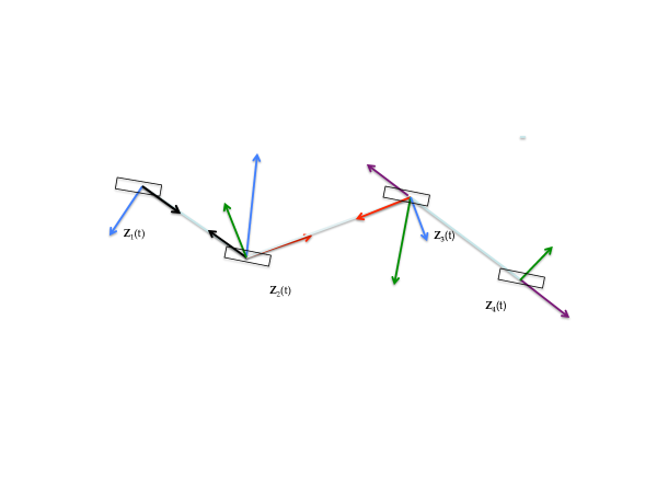
Figure 1: 2-D swimmer consisting of 4 identical rectangles of the same spatial orientation. All possible internal rotational and elastic internal forces are shown (i.e., when swimmer is not in fluid).

Figure 2: 2-D swimmer consisting of 4 identical rectangles which have different spatial orientation. All possible rotational and elastic internal forces are shown (i.e., when swimmer is not in fluid).

We assume that the forcing term $f$ in (1) represents the sum of rotational and elastic(or we can also call them “structural”) forces generated by the swimmer (see cf. Section 12.1 in [9], [13]):

$$f(t,x):=f_{rot}(t,x)+f_{el}(t,x).$$ (4)

More precisely, we assume that any of the intermediate points $z_{i},i=2,\ldots,n-1$ can force the pair of adjacent points $z_{i-1}$ and $z_{i+1}$ to rotate about it, while creating, due to Newton’s 3rd Law, a counterforce acting upon $z_{i}$ itself (see Figure 1):

$$f_{rot}(t,x):=\sum_{i=2}^{n-1}v_{i-1}f_{i-1}(t,x),\;\;z=(z_{1},\ldots,z_{n}),$$ (5)

$$f_{i-1}(t,x)=\bigg{[}\xi_{i-1}(t,x)\,P_{i}[t]\,\big{(}z_{i-1}(t)-z_{i}(t)\big{)}-\xi_{i+1}(t,x)\,{|z_{i-1}(t)-z_{i}(t)|^{2}\over|z_{i+1}(t)-z_{i}(t)|^{2}}\,Q_{i}[t]\,\big{(}z_{i+1}(t)-z_{i}(t)\big{)}\bigg{]}$$

$$+\xi_{i}(t,x)\,\bigg{[}P_{i}[t]\,\big{(}z_{i}(t)-z_{i-1}(t)\big{)}-\,{|z_{i-1}(t)-z_{i}(t)|^{2}\over|z_{i+1}(t)-z_{i}(t)|^{2}}\,Q_{i}[t]\,\big{(}z_{i}(t)-z_{i+1}(t)\big{)}\bigg{]},\;\;i=2,\ldots,n-1.$$ (6)

In the 2-$D$ case we set $P_{i}[t]=Q_{i}[t]=A=\left(\begin{array}[]{cc}0&1\\ -1&0\end{array}\right)$. The functions $v_{1},\ldots,v_{n-2}\in\mathbf{L}^{\infty}(0,T)$ are multiplicative controls (i.e., selectable parameters to control the swimming process).

In the 3-$D$ case, to satisfy the 3rd Newton’s law, we need to make sure that the respective rotational forces acting on $z_{i-1}(t)$ and $z_{i+1}(t)$ lie in the same plane spanned by the vectors $z_{i-1}(t)-z_{i}(t)$ and $z_{i+1}(t)-z_{i}(t)$. In order to achieve the continuity of these forces in time, in this paper we choose to reduce their magnitudes to zero, when the triplet $\{z_{i-1}(t),z_{i}(t),z_{i+1}(t)\}$ approaches the aligned configuration (for other options see [12]). Indeed, such configuration admits infinitely many planes containing this triplet, which makes it an intrinsic point of discontinuity for the procedure of the choice of the rotational plane by means of the rotational forces whose magnitudes are strictly separated from zero. Respectively, we set (see [12]-[13] for more details):

$${\bf x}\mapsto P_{i}[t]{\bf x}:=\big{[}(z_{i-1}(t)-z_{i}(t))\times(z_{i+1}(t)-z_{i}(t))\big{]}\times{\bf x}\,,$$

$${\bf x}\mapsto Q_{i}[t]{\bf x}:={\bf x}\times\big{[}(z_{i-1}(t)-z_{i}(t))\times(z_{i+1}(t)-z_{i}(t))\big{]}\,.$$

Note that $P_{i}[t]{\bf x}=-Q_{i}[t]{\bf x}$ and $|P_{i}[t]{\bf x}|=|Q_{i}[t]{\bf x}|\to 0$ for any ${\bf x}$ when points $z_{i-1}(t),z_{i}(t),z_{i+1}(t)$ converge to the aligned configuration.

In turn,

$$f_{el}(t,x):=\sum_{i=n}^{2n-2}v_{i-1}f_{i-1}(t,x),\;\;z=(z_{1},\ldots,z_{n}),$$ (7)

$$f_{i-1}(t,x):=\xi_{i-1}(t,x)\,\big{(}z_{i}(t)-z_{i-1}(t)\big{)}+\xi_{i}(t,x)\,\big{(}z_{i-1}(t)-z_{i}(t)\big{)},$$ (8)

where the functions $v_{n-1},\ldots,v_{2n-3}\in\mathbf{L}^{\infty}(0,T)$ control the distances respectively between $z_{i}$ and $z_{i-1},i=1,\ldots,n$. We set $v=(v_{1},\ldots,v_{2n-3})$.

Below, we use the following classical notations:

• $\mathbf{C}_{c}^{\infty}(\Omega)$ denotes the space of infinitely many times differentiable functions with compact support in $\Omega$;

• $H^{1}(\Omega)=\{\varphi|\varphi,\varphi_{x_{i}}\in\mathbf{L}^{2}(\Omega),i=1,\ldots,d\}$ and $H^{2}(\Omega)=\{\varphi|\varphi,\varphi_{x_{i}},\varphi_{x_{i}x_{j}}\in\mathbf{L}^{2}(\Omega),i,j=1,\ldots,d\}$;

• $H^{1}_{0}(\Omega)$ denotes the subspace of $H^{1}(\Omega)$ consisting of functions vanishing on $\partial\Omega$.

As in [26], page 5, we also introduce the following classical vector function spaces:

$${\cal V}:=\{\varphi\in[\mathbf{C}_{c}^{\infty}(\Omega]^{d}~{}|~{}\mathrm{div}\,\varphi=0\}\,,d=2,3,$$

$$H:=\mathrm{cl}_{\mathbf{L}^{2}}({\cal V})\,,\qquad\qquad V:=\mathrm{cl}_{H^{1}_{0}}({\cal V})\,=\{\varphi\in[H^{1}_{0}(\Omega)]^{2}~{}|~{}\mathrm{div}\,\varphi=0\}\,,$$

where the symbol $\mathrm{cl}_{\mathbf{L}^{2}}$ stands for the closure with respect to the $[\mathbf{L}^{2}(\Omega)]^{d}$-norm, and $\mathrm{cl}_{H^{1}_{0}}$ – with respect to the $[H^{1}_{0}(\Omega)]^{d}$-norm. The latter is induced by the scalar product

$$[\varphi,\psi]~{}:=\;\sum_{i,j=1}^{d}\mathop{\int}_{\Omega}\varphi_{ix_{j}}\psi_{ix_{j}}dx.\;\;\varphi=(\varphi_{1},\ldots,\varphi_{d}),\;\psi=(\varphi_{1},\ldots,\varphi_{d}).$$

In [13] we proved the following well-posedness results.

Theorem 1 (Well-posedness of model (1)-(8) in the 2-$D$ case)

Let , $z_{1,0},\ldots,z_{n,0}\in\Omega\subset\mathbb{R}^{2}$, $u_{0}\in H$, and $v_{1},\ldots,v_{2n-3}\in\mathbf{L}^{\infty}(0,\hat{T})$ for some $\hat{T}>0$. Assume that

$$\overline{S}(z_{i,0})\subset\Omega,\qquad\qquad|z_{i,0}-z_{j,0}|>2r,\qquad\qquad i,j=1,\ldots,n,~{}~{}i\neq j.$$ (9)

(Assumption (9) ensures that no parts of swimmer’s body overlap with each other and all lie within $\Omega$.) Then, there exists $T^{*}\in(0,\hat{T}]$, depending on $u_{0},z(0)=(z_{1,0},\ldots,z_{n,0})$ and the $\mathbf{L}^{\infty}(0,\hat{T})$-norms of $v_{j}$’s, such that system (1)-(9) admits a unique solution

$$(u,z)\in\bigg{(}C([0,T^{*}];H)\bigcap\mathbf{L}^{2}(0,T^{*};V)\bigg{)}\times[C([0,T^{*}]\,;\mathbb{R}^{2})]^{n},$$

and

$$\overline{S}(z_{i}(t))\subset\Omega,\qquad|z_{i}(t)-z_{j}(t)|>2r,\qquad i,j=1,\ldots,n,~{}~{}i\neq j\,\qquad\forall t\in[0,T^{*}].$$ (10)

The equation (1) in the above is understood in the sense of the following identity:

$$\int_{\Omega}u(x,t)\phi(t)dx-\int_{\Omega}u(x,0)\phi(t)dx-\int_{0}^{t}\int_{\Omega}u\cdot\phi_{t}dxdt\;=$$

$$=-\int_{0}^{t}\nu\,[u(\tau,\cdot),\phi(\tau,\cdot)]dt\;+\;\int_{0}^{t}\int_{\Omega}\bigg{(}-(u\cdot\nabla)u+\,P_{H}f_{j}(\tau,x;h)\bigg{)}\phi dxd\tau,\;\;t\in[0,T^{*}],$$ (11)

where $P_{H}:[\mathbf{L}^{2}(\Omega)]^{d}\rightarrow H$ denotes the projection operator from $[\mathbf{L}^{2}(\Omega)]^{d}$ onto $H$ and $\phi$ is any function such that $\phi\in\Phi=\{\phi\in\mathbf{L}^{2}(0,T^{*};V)$, $\phi_{t}\in\mathbf{L}^{2}(0,T^{*};H)\}$. The complementing $\nabla p=f-u_{t}+\nu\Delta u-(u\cdot\nabla)u$ is understood in the sense of distributions.

Theorem 2 (Well-posedness of model (1)-(8) in 2-$D$ and 3-$D$ cases)

Let $\partial\Omega$ be of class $C^{2}$, $z_{1,0},\ldots,z_{n,0}\in\Omega\subset\mathbb{R}^{d},\;d=2,3$, $u_{0}\in V$, and $v_{1},\ldots,v_{2n-3}\in\mathbf{L}^{\infty}(0,\hat{T})$ for some $\hat{T}>0$. Assume that (9) holds. Then, there exists $T^{*}\in(0,\hat{T}]$, depending on $u_{0},z(0)=(z_{1,0},\ldots,z_{n,0})$ and the $\mathbf{L}^{\infty}(0,\hat{T})$-norms of $v_{j}$’s, such that system (1)-(9) admits a unique solution

$$(u,z)\in C([0,T^{*}];V)\times[C([0,T^{*}]\,;\mathbb{R}^{d})]^{n},\;\;\;\;\nabla p\in[\mathbf{L}^{2}(Q_{T^{*}})]^{d}$$

($\nabla p(t,\cdot)\in H^{\perp}$, the orthogonal complement of $H$ in $[\mathbf{L}^{2}(\Omega)]^{d}$) and

$$\overline{S}(z_{i}(t))\subset\Omega,\qquad|z_{i}(t)-z_{j}(t)|>2r,\qquad i,j=1,\ldots,n,~{}~{}i\neq j\,\qquad\forall t\in[0,T^{*}].$$ (12)

Remark 1.2

The argument of [13] makes use of Schauder’s fixed point theorem. In particular, we showed that the sequence of uncoupled mappings corresponding to the uncoupled version of system (1)-(9), namely: $\;w$ (in place of $u$) $\rightarrow z\rightarrow f\rightarrow u$ are continuos with respect to the norms $\mathbf{L}^{2}(0,T^{*};V)\rightarrow[C([0,T^{*}]\,;\mathbb{R}^{2})]^{n}\rightarrow\mathbf{L}^{2}(0,T^{*};[\mathbf{L}^{2}(\Omega)]^{d})\rightarrow\mathbf{L}^{2}(0,T^{*};V)$ and their product is a compact operator with the unique fixed point $u$.

Remark 1.3 (Some useful estimates)

Solution to (1) satisfies the following estimates (see [15], Lemma 9, p. 194, (55); [16], [26] [13]).

• Under the assumptions of Theorems 1 and 2:

  $$\|u\|_{C(0,T^{*}\,;H)}+\|u\|_{\mathbf{L}^{2}(0,T^{*}\,;V)}\leq\;L_{\bf S_{1}}\left(\,\|u_{0}\|_{H}+\,\|f\|_{\mathbf{L}^{2}(0,T^{*}\,;[\mathbf{L}^{2}(\Omega)]^{d})}\right)$$ (13)

  for some constant $L_{\bf S_{1}}$. Let us also recall here the following estimate from Theorem 11 in [16], see estimates (45) and (48) on pp. 170-171 (see also [13])

  $$\|u_{(1)}-u_{(2)}\|_{C([0,T^{*}];H)}\;+\|u_{(1)}-u_{(2)}\|_{\mathbf{L}^{2}(0,T^{*};V)}\leq\;D^{*}\;\|f_{(1)}-f_{(2)}\|_{\mathbf{L}^{2}(0,T^{*}\,;[\mathbf{L}^{2}(\Omega)]^{d})},$$ (14)

  where $u_{(m)}$ is the solution to (1)-(8) for $f=f_{(m)},m=1,2$ and $D^{*}(s)$ is a nondecreasing function of $\max_{m=1,2}\{\|u_{(m)}\|_{\mathbf{L}^{2}(0,T^{*};V)})\}$.

• Under the assumptions of Theorems 1 and 2:

  $$\|v_{j}f_{j}\|_{[\mathbf{L}^{\infty}(Q_{T^{*}})]^{d}}\;\leq\;C_{\Omega,r}|v_{j}|,\;\;d=2,3,$$ (15)

  for some constant $C_{\Omega,r}>$ depending on $\Omega$ and $r$.

• In tern, under the assumptions of Theorem 2:

  $$\|u\|_{C(0,T^{*}\,;V)}\;\leq\;L_{\bf S_{2}}\left(\,\|u_{0}\|_{V}+\,\|f\|_{\mathbf{L}^{2}(0,T^{*}\,;[\mathbf{L}^{2}(\Omega)]^{d})}\right)$$ (16)

  for some constant $L_{\bf S_{2}}$.

(H3) Everywhere below we assume that the initial datum $u_{0}$ is fixed.

Our first main result describes the micromotions of the swimmer in 2-$D$ and 3-$D$ models (1)-(9) in terms of projections of its internal forces at the initial moment on $H$.

Theorem 3 (Swimmer’s micromotions)

Under the assumptions of Theorems 1 and 2, if we set $v_{j}=ha_{j}\in\mathbb{R},\;\sum_{j=1}^{2n-3}a_{j}^{2}=1,t\in(0,T^{*}),\;\|(v_{1},\ldots,v_{2n-3})\|_{\mathbb{R}^{2n-3}}=|h|\leq 1$ , then

$$z_{i}(t)\;=z_{i}(0)\;+\;{ht^{2}\over{2\mathrm{meas}(S(0))}}\,\sum_{j=1}^{2n-3}a_{j}\int_{S(z_{i}(\tau;0))}(P_{H}f_{j}^{T}(0,\cdot))(x)dx+ht^{2}\rho(t)+h\zeta(h,t),\;\;t\in[0,T^{*}],$$ (17)

where $\|\rho\|_{[C[0,t]]^{d}}=O(t)$, $\|\zeta(h,\cdot)\|_{[C[0,t]]^{d}}=\;O(h)$ ($d=2,3$) and are defined by $u_{0}$ and $f_{j}(0,\cdot)$. (Here and below $O(p)$ denotes a real-valued function that tends to 0 as $\mathbb{R}\ni p\rightarrow 0$.)

The main controllability results of this paper are as follows.

Theorem 4 (Local swimming controllability of $z_{i}$’s: 2-$D$ case)

Given $u_{0}\in H$, under the assumptions of Theorem 1, let $(u^{*},z^{*}=(z_{1}^{*},\ldots,z^{*}_{n}))$ be the solution to (1)-(8) generated by the zero controls $v_{1}=\ldots=v_{2n-3}=0$ on some interval $[0,T^{*}]$. (Note: due to Remark 1.2 and (12), the curves $z^{*}_{i}(t),t\in[0,T^{*}],i=1,\ldots,n$ lie in $\Omega$ along with some their neighborhoods:

$$B_{\mu}(z_{i}^{*}(t))\subset\Omega,\;\;t\in[0,T^{*}],\;\;i=1,\ldots,n,$$ (18)

where $B_{\mu}(z^{*}(t))$ is the ball in $\mathbb{R}^{2}$ with center at $z_{i}^{*}(t)$ of radius $\mu>0$.) Let for some $i\in\{1,\ldots,n\}$ and $k,l\in\{1,\ldots,2n-3\}$ the vectors

$$\int_{S(z_{i}(0))}(P_{H}f_{k}(0,\cdot))(x)\,dx,\;\int_{S(z_{i}(0))}(P_{H}f_{l}(0,\cdot))(x)\,dx$$ (19)

be linearly independent. Then there exist $T=T(i,k,\ell)\in\,(0,T^{*}]$ and $\varepsilon=\varepsilon(i,k,\ell)>0$ such that

$$B_{\varepsilon}(z_{i}^{*}(T))\subseteq\Big{\{}z_{i}(T)~{}|~{}v_{k},v_{\ell}\in\mathbb{R},\;\;{\rm while}\;\;v_{j}=0\;\;{\rm for}\;\;j=1,\ldots,2n-3,~{}j\neq k,\ell\Big{\}}\,.$$

In other words, under the conditions of Theorem 4, the point $z_{i}$ can be steered on some time-interval $[0,T]$ from its initial position $z_{i,0}=z_{i}^{*}(0)$ to any point within the ball $B_{\varepsilon}(z_{i}^{*}(T))$ of radius $\varepsilon>0$ with center at the endpoint $z_{i}^{*}(T)$ of the “drifting” trajectory $z_{i}^{*}(t),t\in[0,T]$. We will also show in our proofs below that this can be achieved merely by constant controls $v_{i}$’s.

At no extra cost (making use of (17) instead of (62)), we will have the following result for the motion of the center of mass of our swimmer.

Theorem 5 (Local swimming locomotion: 2-$D$ case)

Let in Theorem 4 condition (19) is replaced with the following:

$$\sum_{i=1}^{n}\int_{S(z_{i}(0))}(P_{H}f_{k}(0,\cdot))(x)\,dx,\;\sum_{i=1}^{n}\int_{S(z_{i}(0))}(P_{H}f_{l}(0,\cdot))(x)\,dx$$ (20)

are linearly independent. Then the result of Theorem 4 holds with respect to the swimmer’s center of mass $z_{c}=\frac{1}{n}\sum_{i=1}^{n}z_{i}(t)$, namely:

$$B_{\varepsilon}(z_{c}^{*}(T))\subseteq\Big{\{}z_{c}(T)~{}|~{}v_{k},v_{\ell}\in\mathbb{R},\;{\rm while}\;\;v_{j}=0\;\;{\rm for}\;j=1,\ldots,2n-3,~{}j\neq k,\ell\Big{\}},\;z_{c}^{*}=\frac{1}{n}\sum_{i=1}^{n}z_{i}^{*}(t).$$

Theorem 6 (Local controllabity in 3-$D$)

Given $u_{0}\in V$, under the assumptions of Theorem 2, the results of Theorem 4 can be extended to the case of 3-$D$ swimming model (1)-(8), assuming that three controls $v_{k},v_{l}$ and $v_{m}$ are active (i.e., in place of two as in Theorem 4).

Theorem 7 (Local locomotion in 3-$D$)

Given $u_{0}\in V$, under the assumptions of Theorem 2, the results of Theorem 5 hold for the case of 3-$D$ swimming model (1)-(8) for three active controls $v_{k},v_{l}$ and $v_{m}$ (i.e., in place of two as in Theorem 5).

The main idea of our proofs below is to show that each of the mappings

$$\mathbb{R}^{2}\ni(v_{k},v_{l})\;\rightarrow\;z_{i}(T)\in\mathbb{R}^{2},\;\;\;\mathbb{R}^{3}\ni(v_{k},v_{l},v_{m})\;\rightarrow\;z_{i}(T)\in\mathbb{R}^{3},$$ (21)

associated with Theorems 4 and 6, considered on some (open) neighborhood of the origin, is 1-1 and its range contains an open neighborhood of $z_{i}^{*}(T)$ for some $T>0$. To this end, we intend to study the invertibility properties of the respective $[2\times 2]$- and $[3\times 3]$-matrices:

$$\left(\frac{dz_{i}(T)}{dv_{k}}\mid_{v_{j}^{\prime}s=0},\frac{dz_{i}(T)}{dv_{l}}\mid_{v_{j}^{\prime}s=0}\right)$$

$$\left(\frac{dz_{i}(T)}{dv_{k}}\mid_{v_{j}^{\prime}s=0},\frac{dz_{i}(T)}{dv_{l}}\mid_{v_{j}^{\prime}s=0},\frac{dz_{i}(T)}{dv_{m}}\mid_{v_{j}^{\prime}s=0}\right).$$ (22)

In the above and anywhere below the subscript $v_{j}^{\prime}s=0$ indicates that the corresponding expressions are calculated for $\;v_{j}=0,j=1,\ldots,2n-3$.

The remainder of the paper is organized as follows. Sections 2 and 3 deal with detailed proofs of auxiliary results in the 2-$D$ case. Namely, in Section 2 we will describe the derivatives ${\partial u\over\partial v_{j}}|_{v_{j}^{\prime}s=0},j=1,\ldots,2n-3$ as solutions to some linear system of partial differential equations. Then in Section 3 we will show that the derivatives ${\partial z_{i}\over\partial v_{j}}|_{v_{j}^{\prime}s=0},i=1,\ldots,n,\;j=1,\ldots,2n-3$ satisfy a system of integral Volterra equations. In Section 4 we will prove Theorem 3 and the main controllability results for the 2-$D$ case. In Section 5 we show how they can be extended to the 3-$D$ case. In Section 6 we discuss illustrating examples.

Prior related results on swimming controllability. Local controllability results similar to Theorems 4 and 5 were obtained in [7] (see also [9], Ch. 14) for the case of an incompressible fluid governed by the non-stationary Stokes equations and when the elastic forces were described by “uncontrollable” Hooke’s Law. The proofs in [7] were based on the Inverse Function Theorem for the 2-$D$ mapping (21) and employed the linearity of the fluid equations to represent the velocity of fluid in the form of implicit Fourier series expanded along the associated set of eigenfunctions. In this paper we follow the general strategy of [7]. However, the nonlinearity of Navier-Stokes equations requires a principal modification of this strategy and its setup. In particular, in (7)-(8) we consider controlled elastic forces instead of Hooke’s Law as in [7]. For such forces in [9], Ch. 15 we obtained some global controllability results for the case a swimmer applying a rowing-type motion in a fluid governed by the non-stationary Stokes equations (see also [11] for the 3-$D$ case).

Remark 1.4 (Swimming controllability in the framework of ODE’s)

A number of attempts were made to study controllability of various “ swimmers” in the context of swimming models in the framework of ODE’s, see, e.g., Koiller et al. [14] (1996); McIsaac and Ostrowski [19] (2000); Martinez and Cortes [20] (2001); Trintafyllou et al. [27] (2000); Alouges et al. [1] (2008), Sigalotti and Vivalda [23] (2009), and the references therein.

2 Derivatives ${\partial u\over\partial v_{j}}|_{v_{j}^{\prime}s=0}$: 2-$D$ case

As suggested by the representaion of matrices in (22), we intend to evaluate the derivatives ${d\over dv_{j}}\,z_{i}(t)$ assuming that $v_{j}$’s are independent variables (real numbers) in (1)-(2). As the 1st step in this direction, in this section we will study derivatives ${\partial u\over\partial v_{j}}|_{v_{j}^{\prime}s=0}$.

Fix any $j\in\{1,\dots,2n-3\}$ and assume that in (1)-(8)

$$v_{j}=h\in\mathbb{R},\;\;|h|\leq 1,\;\;v_{m}=0,\;\;m\neq j,$$ (23)

denoting respectively in this case:

$$z_{i}(t)=z_{i}(t;h),\;\;z(t)=z(t;h),\;\;f(t,x)=f(t,x;h),\;\;f_{j}(t,x)=f_{j}(t,x;h),\;p(t,x)=p(t,x;h),$$

$$u(t,x)=u(t,x;h)=u_{h}(t,x),\;\;u_{*}(t,x)=u(t,x;0),\;\;w_{h}=\,\frac{u_{h}-u_{*}}{h}.$$ (24)

We will study the behavior of $w_{h}$ as $h$ tends to zero. Then, (1) yields:

$$\left\{\begin{array}[]{ll}w_{ht}=\nu\,\Delta w_{h}-(u_{*}\cdot\nabla)w_{h}-(w_{h}\cdot\nabla)u_{h}\\ +\;\,f_{j}(\cdot,\cdot;h)-{1\over h}\nabla(p(\cdot,\cdot;h)-p(\cdot,\cdot;0))&\mbox{ in }(0,T^{*})\times\Omega,\\ \mathrm{div}\,w_{h}=0&\mbox{ in }(0,T^{*})\times\Omega,\;{\rm i.e.},\;w_{h}(t,\cdot)\in H,\\ w_{h}=0&\mbox{ in }(0,T^{*})\times\partial\Omega,\\ w_{h}(0,\cdot)=0&\mbox{ in }\Omega.\end{array}\right.$$ (25)

By Theorem 1, (6), (8) and due to continuous embedding (for $\Omega\subset\mathbb{R}^{2}$, see Remark 2.1 below)

$$C([0,T^{*}];[\mathbf{L}^{2}(\Omega)]^{2})\bigcap\mathbf{L}^{2}([0,T^{*};V)\;\subset[\mathbf{L}^{4}(Q_{T^{*}})]^{2}=[\mathbf{L}_{4,4}(Q_{T^{*}})]^{2},$$ (26)

we have:

$$u_{*},u_{h},w_{h}\in C([0,T^{*}];H)\bigcap\mathbf{L}^{2}(0,T^{*};V)\bigcap[\mathbf{L}^{4}(Q_{T^{*}})]^{2},\;\;f_{j}(\cdot,\cdot;h)\in[\mathbf{L}^{\infty}(Q_{T^{*}})]^{2}.$$ (27)

Remark 2.1

In the above we used estimate (3.4) in [17], page 75, namely:

$$\|\psi\|_{\mathbf{L}^{4}(Q_{t})}\;\leq\;\beta\bigg{(}\max_{\tau\in[0,t]}\|\psi(\tau,\cdot)\|_{\mathbf{L}^{2}(\Omega)}+\|\nabla\psi\|_{[\mathbf{L}^{2}(Q_{t})]^{2}}\bigg{)}.$$ (28)

We claim that Theorem 1.1 in [17], pages 573-574 on well-posednes of general parabolic systems (see Remark 2.2 below) implies that (25) admits a unique solution of regularity described in (27) and for some constant $C^{*}>0$ the following estimate holds:

$$\|w_{h}\|_{C([0,T^{*}];[\mathbf{L}^{2}(\Omega)]^{2})\bigcap\mathbf{L}^{2}([0,T^{*};V)}\mathop{=}^{\Delta}\;\max_{t\in[0,T^{*}]}\|w_{h}(t,\cdot)\|_{[\mathbf{L}^{2}(\Omega)]^{2}}$$

$$+\|w\|_{\mathbf{L}^{2}(0,T^{*};V)}\;\leq C^{*}\|Pf_{j}(\cdot,\cdot;h)\|_{[\mathbf{L}_{2,1}(Q_{T^{*}})]^{2}}\leq C^{*}\|f_{j}(\cdot,\cdot;h)\|_{[\mathbf{L}_{2,1}(Q_{T^{*}})]^{2}}.$$ (29)

Indeed, the proof of this theorem is based on Galerkin methods with test functions

$$\phi\in\mathbf{L}^{2}(0,T^{*};[H_{0}^{1}(\Omega)]^{2})\bigcap\{\phi(\cdot,x)\in[H^{1}(0,T^{*})]^{2}\;{\rm\;a.e.\;in}\;\Omega\},$$

see [17]. However, in the case of the special mixed problem (25), including the extra condition that $\mathrm{div}\,w_{h}=0$, we are dealing with $w_{h}(t,\cdot)$ that lie in $V$ for almost all $t$, see (27). Therefore, $w_{h}$ can be represented as a Fourier series expanded only along the eigenfunctions $\{\omega_{k}\}_{k=1}^{\infty},\omega_{k}\in V,k=1,\ldots$ of the spectral problem associated with (1), forming a complete orthogonal basis in $V$ and orthonormal in $H$ ([16]), namely, in the following form:

$$w_{h}(t,x)=\sum_{k=1}^{\infty}c_{k}(t)\omega_{k}(x);\;\;\;\;\nu\Delta\omega_{k}=\lambda_{k}\omega_{k}+\nabla p_{k},\;\mathrm{div}\,\omega_{k}=0\;\;{\rm in}\;\Omega,\;\;k=1,\ldots.$$ (30)

The equation for $\omega_{k}$’s is understood in the sense of identity (see also (31))

$$-\nu\,[w_{k},\phi]\;=\;\lambda_{k}\int_{\Omega}\omega_{k}\phi dxd\tau\;\;\;\;\forall\phi\in V.$$

In other words, (25) is equivalent to the following identity obtained as the difference of identities (11) in the cases when $u=u_{h}$ and $u=u_{*}$ and then divided by $h$ (compare to [17], p. 572):

$$\int_{\Omega}w_{h}(x,t)\phi(t)dx-\int_{0}^{t}\int_{\Omega}w_{h}\cdot\phi_{t}dxdt\;=$$

$$=-\int_{0}^{t}\nu\,[w_{h}(\tau,\cdot),\phi(\tau,\cdot)]dt\;+\;\int_{0}^{t}\int_{\Omega}\bigg{(}-(u_{*}\cdot\nabla)w_{h}-(w_{h}\cdot\nabla)u_{h}+\,P_{H}f_{j}(\tau,x;h)\bigg{)}\phi dxd\tau,\;\;t\in[0,T^{*}],$$ (31)

where $\phi$ is any function such that $\phi\in\Phi=\{\phi\in\mathbf{L}^{2}(0,T^{*};V)$, $\phi_{t}\in\mathbf{L}^{2}(0,T^{*};H)\}$.

The derivation of (29) in [17] is based on the classical form of identity (31), namely, with any $\phi\in\mathbf{L}^{2}(0,T^{*};[H_{0}^{1}(\Omega)]^{2}),\phi_{t}\in\mathbf{L}^{2}(Q_{T^{*}})$, which in this case will be applied for $\phi\in\Phi$, and, thus, is the same as just to use the last line in (31) from the start.

Remark 2.2

Let us recall the following results from [17].

• Theorem 1.1 in [17], pages 573 requires that the squared 1-$D$ components of the 2-$D$ vector-function $u_{*}$ and 1-$D$ components of the $2\times 2$ matrix-function $\nabla u_{h}$ (as the coefficients in (25)) are elements of the space $\mathbf{L}_{q,r}(Q_{T^{*}})$, where

  $$\|\psi\|_{\mathbf{L}_{q,r}(Q_{T^{*}})}\;=\;\bigg{(}\int_{0}^{T^{*}}\bigg{(}\int_{\Omega}|\psi|^{q}dx\bigg{)}^{r/q}dt\bigg{)}^{1/r},\;\;\frac{1}{r}+\frac{1}{q}=1,\;\;q\in(1,\infty],\;r\in[1,\infty),$$

  while the free term $f_{j}(\cdot,\cdot;h)$ lies in $\mathbf{L}_{q_{1},r_{1}}(Q_{T^{*}})$ (due to (31) we ignore the term $-{1\over h}\nabla(p(\cdot,\cdot;h)-p(\cdot,\cdot;0))$ here), where $\frac{1}{r_{1}}+\frac{1}{q_{1}}=1+\frac{1}{2},\;q_{1}\in(1,2],\;r_{1}\in[1,2)$. We can select $r_{1}=1,q_{1}=2$ and $r=2=q$.

• Constant $C^{*}$ can be selected to be dependent only on $\|u_{*}\|_{C([0,T^{*}];[\mathbf{L}^{2}(\Omega)]^{2})\bigcap\mathbf{L}^{2}([0,T^{*};V)}$ or $\|u_{*}\|_{[\mathbf{L}^{4}(Q_{T^{*}})]^{2}}$, and $\|\nabla u_{h}\|_{[[\mathbf{L}^{2}(Q_{T^{*}})]^{2}]^{2}},\,|h|\leq 1$, see [17], pages 573-574 and (23).

• Condition $\mathrm{div}\,w_{h}=0$ is not required in Theorem 1.1 in [17], page 573.

• Note that $w_{h}$ also satisfy the regularity of solutions to (1) described in Theorem 1.

Based on the above discussion, we can refine (29) as follows:

$$\|w_{h}\|_{C([0,T^{*}];[\mathbf{L}^{2}(\Omega)]^{2})\bigcap\mathbf{L}^{2}([0,T^{*};V)}\;\leq C^{*}\|f_{j}(\cdot,\cdot;h)\|_{[\mathbf{L}_{2,1}(Q_{T^{*}})]^{2}}$$

$$\leq C^{*}T^{*}\,{\rm meas}^{1/2}\,(\Omega)\,\|f_{j}(\cdot,\cdot;h)\|_{[\mathbf{L}^{\infty}(Q_{T^{*}})]^{2}}\;\leq\;C^{*}T^{*}\,{\rm meas}^{1/2}\,(\Omega)\,C_{\Omega,r},\;\;j=1,\ldots,2n-3.$$ (32)

Introduce the following linear system:

$$\left\{\begin{array}[]{ll}\bigg{(}{\partial u\over\partial v_{j}}|_{v_{j}^{\prime}s=0}\bigg{)}_{t}\;=\;\nu\,\Delta\bigg{(}{\partial u\over\partial v_{j}}|_{v_{j}^{\prime}s=0}\bigg{)}-(u_{*}\cdot\nabla)\bigg{(}{\partial u\over\partial v_{j}}|_{v_{j}^{\prime}s=0}\bigg{)}\\ -(\bigg{(}{\partial u\over\partial v_{j}}|_{v_{j}^{\prime}s=0}\bigg{)}\cdot\nabla)u_{*}+\,P_{H}f_{j}(\cdot,\cdot;0)-\nabla p_{j}&\mbox{ in }(0,T^{*})\times\Omega,\\ \mathrm{div}\,\bigg{(}{\partial u\over\partial v_{j}}|_{v_{j}^{\prime}s=0}\bigg{)}=0&\mbox{ in }(0,T^{*})\times\Omega,\\ &\;{\rm i.e.},\;\bigg{(}{\partial u\over\partial v_{j}}|_{v_{j}^{\prime}s=0}\bigg{)}(t,\cdot)\in H,\\ \bigg{(}{\partial u\over\partial v_{j}}|_{v_{j}^{\prime}s=0}\bigg{)}=0&\mbox{ in }(0,T^{*})\times\partial\Omega,\\ \bigg{(}{\partial u\over\partial v_{j}}|_{v_{j}^{\prime}s=0}\bigg{)}(0,\cdot)=0&\mbox{ in }\Omega,\end{array}\right.$$ (33)

where (in the sense of distributions, see also Theorem 1),

$$\nabla p_{j}=$$

$$-\bigg{(}{\partial u\over\partial v_{j}}|_{v_{j}^{\prime}s=0}\bigg{)}_{t}+\nu\,\Delta\bigg{(}{\partial u\over\partial v_{j}}|_{v_{j}^{\prime}s=0}\bigg{)}-(u_{*}\cdot\nabla)\bigg{(}{\partial u\over\partial v_{j}}|_{v_{j}^{\prime}s=0}\bigg{)}-(\bigg{(}{\partial u\over\partial v_{j}}|_{v_{j}^{\prime}s=0}\bigg{)}\cdot\nabla)u_{*}+P_{H}f_{j}(\cdot,\cdot;0).$$

Remark 2.3 (On understanding system (33))

Due to incompressibility (“divergence-free”) condition

$$\mathrm{div}\,\bigg{(}{\partial u\over\partial v_{j}}|_{v_{j}^{\prime}s=0}\bigg{)}=0,$$

similar to (30), we can represent solution to (33) as the series

$$\bigg{(}{\partial u\over\partial v_{j}}|_{v_{j}^{\prime}s=0}\bigg{)}(t,x)=\sum_{k=1}^{\infty}d_{k}(t)\omega_{k}(x).$$ (34)

Then the argument of the classical theory of parabolic pde’s ([17], Chapters VII and III) can be applied to the “cut-off” form (34) exactly as it is applied in the case when such condition is absent. Respectively, exactly as in the aforementioned classical theory, making use of the identity like (31), we can derive the existence of solution to (33) in $C([0,T^{*}];[\mathbf{L}^{2}(\Omega)]^{2})\bigcap\mathbf{L}^{2}([0,T^{*};V)$ satisfying (36).

Lemma 2.1

Derivatives

$$\lim_{h\rightarrow 0}w_{h}\mathop{=}^{\Delta}{\partial u\over\partial v_{j}}|_{v_{j}^{\prime}s=0},\;\;\;\;j=1,\ldots,2n-3,$$

where the limit is taken with respect to the $C([0,T^{*}];[\mathbf{L}^{2}(\Omega)]^{2})\bigcap\mathbf{L}^{2}([0,T^{*};V)$-norm, exist as unique solutions to (33) and

$${\partial u\over\partial v_{j}}|_{v_{j}^{\prime}s=0}\;\in\;C([0,T^{*}];H)\bigcap\mathbf{L}^{2}(0,T^{*};V)\bigcap[\mathbf{L}^{4}(Q_{T^{*}})]^{2}.$$ (35)

As a particular case of (32), the following estimates hold:

$$\|{\partial u\over\partial v_{j}}|_{v_{j}^{\prime}s=0}\|_{C([0,T^{*}];H)\bigcap\mathbf{L}^{2}(0,T^{*};V)}\;$$

$$\leq C^{*}T^{*}\,{\rm meas}^{1/2}\,(\Omega)\,\|f_{j}(\cdot,\cdot;0)\|_{[\mathbf{L}^{\infty}(Q_{T^{*}})]^{2}}\;\leq\;C^{*}T^{*}\,{\rm meas}^{1/2}\,(\Omega)\,C_{\Omega,r},\;\;j=1,\ldots,2n-3.$$ (36)

where $C^{*}$ can be selected to be dependent only on $\|u_{*}\|_{[\mathbf{L}^{4}(Q_{T^{*}})]^{2}}$ and $\|\nabla u_{*}\|_{[\mathbf{L}^{2}(Q_{T^{*}})]^{2}}$.

Proof:

Step 1. We can use here an adoptation of the argument of Theorem 4.5 in [17], page 166 (on continuous dependence of solutions to parabolic pde’s on coefficients and free terms) to the case of systems of linear parabolic pde’s along Remark 2.3. Namely, denote

$$W_{h}=w_{h}-{\partial u\over\partial v_{j}}|_{v_{j}^{\prime}s=0}.$$

Then, we will have the following identity for $W_{h}$ from (31):

$$\int_{\Omega}W_{h}(x,t)\phi(t)dx-\int_{0}^{t}\int_{\Omega}W_{h}\cdot\phi_{t}dxdt\;$$

$$=-\int_{0}^{t}\nu\,[W_{h}(\tau,\cdot),\phi(\tau,\cdot)]dt\;+\;\int_{0}^{t}\int_{\Omega}\bigg{(}-(u_{*}\cdot\nabla)W_{h}-(W_{h}\cdot\nabla)u_{*}\bigg{)}\phi dxd\tau$$

$$+\;\int_{0}^{t}\int_{\Omega}\bigg{(}F_{h}\;+\,P_{H}(f_{j}(\tau,x;h)-f_{j}(\tau,x;0))\bigg{)}\phi dxd\tau,\;\;t\in[0,T^{*}]$$ (37)

where $F_{h}=(w_{h}\cdot\nabla)(u_{*}-u_{h})$. Then, making use of Remark 2.2 (see also calculations in Step 2 of subsection 4.2 below), we can derive, similar to (29) and [17], page 167:

$$\|W_{h}\|_{C([0,T^{*}];[\mathbf{L}^{2}(\Omega)]^{2})\bigcap\mathbf{L}^{2}([0,T^{*};V)}$$

$$\leq C^{*}\|f_{j}(\tau,x;h)-f_{j}(\tau,x;0)\|_{[\mathbf{L}_{2,1}(Q_{T^{*}})]^{2}}+C^{*}\|F_{h}\|_{[\mathbf{L}_{q_{2},r_{2}}(Q_{T^{*}})]^{2}},$$ (38)

where $q_{2}=2q/(q+1)=4/3,r_{2}=2r/(r+1)=4/3$ and $C^{*}$ is from (36). In turn, see again (68) in subsection 4.2 below:

$$\|F_{h}\|_{[\mathbf{L}_{q_{2},r_{2}}(Q_{T^{*}})]^{2}}\;\leq\;K\|\nabla u_{*}-\nabla u_{h}\|_{[[\mathbf{L}^{2}(Q_{T^{*}})]^{2}]^{2}}\|w_{h}\|_{[\mathbf{L}^{4}(Q_{T^{*}})]^{2}}$$

$$\leq\;K_{*}\|\nabla u_{*}-\nabla u_{h}\|_{[[\mathbf{L}^{2}(Q_{T^{*}})]^{2}]^{2}}T^{*}\,{\rm meas}^{1/2}(\Omega)C_{\Omega,r},$$ (39)

where $K_{*}>0$ is some constant and we used (67) and (28) to derive the 2nd inequality.

Step 2. Note next that, due to (3)-(8), Remarks 1.2 and 1.3, (see (14) and (15)), for some constant $k_{r}$, depending on $r$,

$$\|u_{*}-u_{h}\|_{C([0,T^{*}];H)}+\|\nabla u_{*}-\nabla u_{h}\|_{[[\mathbf{L}^{2}(Q_{T^{*}})]^{2}]^{2}}\;\leq D^{*}\|0\cdot f_{j}(\cdot,\cdot;0)-hf_{j}(\cdot,\cdot;h)\|_{[\mathbf{L}_{2}(Q_{T^{*}})]^{2}}$$

$$\leq\;D^{*}\sqrt{T^{*}}\,{\rm meas}^{1/2}\,(\Omega)\,C_{\Omega,r}|h|\rightarrow\;0\;\;\;\;{\rm as}\;\;h\rightarrow 0,$$

$$\|f_{j}(\cdot,\cdot;h)-f_{j}(\cdot,\cdot;0)\|_{[\mathbf{L}_{2,1}(Q_{T^{*}})]^{2}}\;\leq\;T^{*}\,{\rm meas}^{1/2}\,(\Omega)\,\|f_{j}(\cdot,\cdot;h)-f_{j}(\cdot,\cdot;0)\|_{[\mathbf{L}^{\infty}(Q_{T^{*}})]^{2}}$$

$$\leq\;k_{r}T^{*}\,{\rm meas}^{1/2}\,(\Omega)\,\|z(\cdot;h)-z(\cdot;0)\|_{[C([0,T^{*}];\mathbb{R}^{2})]^{n}}\leq\;k_{r}(T^{*})^{2}\,{\rm meas}\,(\Omega)\,\|u_{*}-u_{h}\|_{C([0,T^{*}];H)}$$

$$\leq\;D^{*}k_{r}(T^{*})^{2.5}\,{\rm meas}^{3/2}\,(\Omega)\,C_{\Omega,r}|h|\;\rightarrow\;0\;\;\;\;{\rm as}\;\;h\rightarrow 0.$$ (40)

Step 3. Estimates (38)- (40) yield that

$$\|w_{h}-{\partial u\over\partial v_{j}}|_{v_{j}^{\prime}s=0}\|_{C([0,T^{*}];H)\bigcap\mathbf{L}^{2}(0,T^{*};V)}\;\leq\;{\cal C}(r,\Omega,T^{*})|h|\;\rightarrow 0\;\;{\rm as}\;h\rightarrow 0,$$ (41)

where ${\cal C}(r,\Omega,T^{*})>0$ is defined by $r,\Omega,T^{*}$ and

$${\cal C}(r,\Omega,T^{*})\rightarrow\;\;{\rm as}\;T^{*}\rightarrow 0.$$ (42)

This completes the proof of Lemma 2.1. $\diamond$

Remark 2.4

We would like to note here that the convergence rate in (41) is linear with respect to $|h|$.

3 Derivatives ${\partial z_{i}\over\partial v_{j}}|_{v_{j}^{\prime}s=0}$ as solutions to Volterra equations: 2-$D$ case

We intend to show that

$${\partial z_{i}\over\partial v_{j}}|_{v_{j}^{\prime}s=0}\;\mathop{=}^{\Delta}\;\lim_{h\rightarrow 0}\frac{z_{i}(t;h)-z_{i}(t;0)}{h},$$

where the limit is taken in $[C[0,T^{*}]]^{2}$-norm exists. To this end, we will use the integral form of equations (2):

$$z_{i}(t;h)=z_{i,o}+\,{1\over\mathrm{meas}(S(0))}\,\int_{0}^{t}\int_{z_{i}(\tau;h)+S(0)}u(\tau,x;h)\,dx\,d\tau$$

$$=z_{i,o}+\,{1\over\mathrm{meas}(S(0))}\,\int_{0}^{t}\int_{S(0)}u(\tau,x-z_{i}(\tau;h);h)\,dx\,d\tau.$$

Respectively:

$$\frac{z_{i}(t;h)-z_{i}(t;0)}{h}\;$$

$$=\,{1\over\mathrm{meas}(S(0))}\,\int_{0}^{t}\int_{S(0)}\frac{u(\tau,x-z_{i}(\tau;h);h)-u(\tau,x-z_{i}(\tau;0);0)}{h}\,dx\,d\tau$$

$$=\,{1\over\mathrm{meas}(S(0))}\,\int_{0}^{t}\int_{S(0)}\frac{u(\tau,x-z_{i}(\tau;h);h)-u(\tau,x-z_{i}(\tau;0);h)}{h}\,dx\,d\tau\;$$

$$+\;{1\over\mathrm{meas}(S(0))}\,\int_{0}^{t}\int_{S(0)}\frac{u(\tau,x-z_{i}(\tau;0);h)-u(\tau,x-z_{i}(\tau;0);0)}{h}\,dx\,d\tau.$$ (43)

In the previous section we studied the integrand in the 2nd term (i.e., $w_{h}$ and its limit properties as $h\rightarrow 0$)), see Lemma 2.1.

Evaluation of the integrand in the 1st term on the right in (43). Due to assumption (18) and Remark 1.2, without loss of generality (namely, for sufficiently small $h$), we can assume that for some $\mu>0$ $z_{i}(t;h)\in B_{\mu}(z_{i}(t;0))\subset\Omega,\;t\in[0,T^{*}]$ and

$$\rho(s,t,x)\;\mathop{=}^{\Delta}\;(1-s)(x-z_{i}(t;0))+s(x-z_{i}(t;h))$$

$$=x-[(1-s)(z_{i}(t;0)+sz_{i}(t;h))]\in\Omega,s\in[0,1],\;x\in S(0),\;t\in[0,T^{*}].$$

We claim that, due to assumption (3) and Remarks 1.2 and 1.3:

$$u(t,x-z_{i}(t;h);h)-u(\tau,x-z_{i}(t;0);h)$$

$$=\;u_{x}(t,x-z_{i}(t;0);0)(z_{i}(t;0))-z_{i}(t;h))\;+\;G(t,x;h)(z_{i}(t;0))-z_{i}(t;h)),$$ (44)

where $u_{x}$ is the Jacobian matrix of the function $u(t,x)$ with respect to $x$ and

$$\|\int_{S(0)}G(t,x;h)dx\|_{\mathbb{R}^{2}}\leq O(h)\|\nabla u(t,\cdot;h)\|_{[[\mathbf{L}^{2}(\Omega)]^{2}]^{2}}\;\;{\rm as}\;h\rightarrow 0,\;\;t\in[0,T^{*}].$$ (45)

Remark 3.1

Here and below, when we use a term like $O(p)$ we assume that it may depends on the given parameters in the original problem (such as $T^{*},\Omega,r,u_{0},v_{i}$’s, selected indeces) but the limit property $O(p)\rightarrow 0$ as $p\rightarrow 0$ holds uniformly over such fixed parameters.

Indeed, for example, if $u=(u_{1},u_{2}),z_{i}=(z_{i1},z_{i2})$, then:

$$u_{1}(t,\rho(1,t,x);h)-u_{1}(t,\rho(0,t,x);h)=u_{1}(t,x-z_{i}(t;h);h)-u_{1}(t,x-z_{i}(t;0);h)\;$$

$$=\;u_{1x_{1}}(t,\rho(s_{1},t,x);h)(z_{i1}(t;0))-z_{i,1}(t;h))\;+u_{1x_{2}}(t,\rho(s_{1},t,x);h)(z_{i2}(t;0))-z_{i,2}(t;h)),$$

where $s_{1}\in[0,1]$ and point $\rho(s_{1},t,x)$ lies in the line interval connecting points $x-z_{i}(t;0)$ and $x-z_{i}(t;h)$ whose length tends to zero as $h\rightarrow 0$ due to Remark 1.2. Then,

$$|\int_{S(0)}(u_{1x_{1}}(t,\rho(s_{1},t,x);h)-u_{1x_{1}}(t,\rho(0,t,x);h))\,dx|\$$

$$=\;|\int_{S(0)}(u_{1x_{1}}(t,\rho(s_{1},t,x);h)-u_{1x_{1}}(t,x-z_{i}(t;0);h))\,dx|$$

$$=\;|\int_{S(\rho(s_{1},t,x)}u_{1x_{1}}(t,x;h)\,dx\;-\;\int_{S(z_{i}(t;0))}u_{1x_{1}}(t,x;h)\,dx|$$

$$\leq\;|\int_{S(\rho(s_{1},t,x))\backslash S(z_{i}(t;0))}|u_{1x_{1}}(t,x;h)|\,dx|\;+\;\int_{S(z_{i}(t;0))\backslash S(\rho(s_{1},t,x))}|u_{1x_{1}}(t,x;h)|\,dx|$$

$$\leq\;\mathrm{meas}(S(\rho(s_{1},t,x))\backslash S(z_{i}(t;0)))^{1/2}\|u_{1x_{1}}(t,\cdot;h)\|_{\mathbf{L}^{2}(\Omega)}\;$$

$$+\;\mathrm{meas}(S(z_{i}(t;0))\backslash S(\rho(s_{1},t,x))))^{1/2}\|u_{1x_{1}}(t,\cdot;h)\|_{\mathbf{L}^{2}(\Omega)}.$$

In turn, combining (3) and Remark 1.3 yields (45).

Volterra equations. Combining (43) and (44) yields the following Volterra equation for $\psi_{h}=\frac{z_{i}(\cdot;h)-z_{i}(\cdot;0)}{h}$:

$$((I+{\mathbb{A}}+{\mathbb{A}_{h}})\psi_{h})(t)\;\mathop{=}^{\Delta}\;\psi_{h}(t)+\int_{0}^{t}\bigg{(}{\mathbb{K}}_{0}(t,\tau)+{\mathbb{K}}_{h}(t,\tau)\bigg{)}\psi_{h}(\tau)d\tau=g(t;h),$$ (46)

$$I+{\mathbb{A}}+{\mathbb{A}}_{h}:[C[0,T^{*}]]^{2}\rightarrow[C[0,T^{*}]]^{2},$$

where $I$ is the identity operator and

$${\mathbb{K}}_{0}(t,\tau)\;=\;{-1\over\mathrm{meas}(S(0))}\,\int_{S(0)}u_{x}(\tau,x-z_{i}(\tau;0);0)dx,\;\;{\mathbb{K}}_{0}\in\mathbf{L}^{2}((0,T^{*})\times(0,T^{*})),$$ (47)

$${\mathbb{K}}_{h}(t,\tau)\;=\;{-1\over\mathrm{meas}(S(0))}\,\int_{S(0)}G(\tau,x;h)dx,$$ (48)

$$g(t;h)\;=\;{1\over\mathrm{meas}(S(0))}\,\int_{0}^{t}\int_{S(0)}{\partial u\over\partial v_{j}}|_{v_{j}^{\prime}s=0}(\tau,x-z_{i}(\tau;0))\,dx\,d\tau\;+\;H(t;h)$$

$$H(t;h)\;=\;{1\over\mathrm{meas}(S(0))}\,\int_{0}^{t}\int_{S(0)}\frac{u(\tau,x-z_{i}(\tau;0);h)-u(\tau,x-z_{i}(\tau;0);0)}{h}\,dx\,d\tau\;$$

$$-\;{1\over\mathrm{meas}(S(0))}\,\int_{0}^{t}\int_{S(0)}{\partial u\over\partial v_{j}}|_{v_{j}^{\prime}s=0}(\tau,x-z_{i}(\tau;0))\,dx\,d\tau,\;\|H(\cdot;h)\|_{C([0,T^{*}];\mathbb{R}^{2})}\rightarrow 0\;{\rm as}\;h\rightarrow 0.$$ (49)

The latter limit property is due to Lemma 2.1. It is well-known that operator $I+{\mathbb{A}}+{\mathbb{A}}_{h}$ in (46) is bijective and has bounded inverse due to the Open Mapping Theorem. Recall that in (23) we assumed that $|h|\leq 1$.

Assumption on $T^{*}$. Recall that in (23) we assumed that $|h|\leq 1$. Without loss of generality, from now on, we can assume that $T^{*}$ is small enough to ensure (making use of estimates in Remark 1.3) that

$$\|{\mathbb{A}}\|<\frac{1}{4},\;\;\;\;\|{\mathbb{A}}_{h}\|<\frac{1}{4}\;\;\;\;\forall|h|\leq 1.$$ (50)

Respectively, in this case, there exists a constant $M_{o}$ such that

$$\|\psi_{h}\|_{C([0,T^{*}];\mathbb{R}^{2})}\;\leq\;M_{o},\;\;|h|\leq 1.$$

Hence, in view of (45), (49) and (41), we can pass to the limit in (46), described as

$$\psi_{h}=\bigg{(}I+{\mathbb{A}}\bigg{)}^{-1}\bigg{(}g(t;h)-{\mathbb{A}}_{h}\psi_{h}\bigg{)}\;=\;\bigg{(}\sum_{k=0}^{\infty}{\mathbb{A}}^{k}\bigg{)}\bigg{(}g(t;h)-{\mathbb{A}}_{h}\psi_{h}\bigg{)},$$

in the $[C[0,T^{*}]]^{2}$-norm as $h\rightarrow 0$ to obtain the existence of

$${\partial z_{i}(t)\over\partial v_{j}}|_{v_{j}^{\prime}s=0}\;=\;\lim_{h\rightarrow 0}\frac{z_{i}(t;h)-z_{i}(t;0)}{h}$$

as the unique solution to the following limit Volterra equation:

$${\partial z_{i}(t)\over\partial v_{j}}|_{v_{j}^{\prime}s=0}\;=-\,\int_{0}^{t}\bigg{\{}{1\over\mathrm{meas}(S(0))}\,\int_{S(0)}u_{x}(\tau,x-z_{i}(\tau;0);0)dx\bigg{\}}\bigg{[}{\partial z_{i}(\tau)\over\partial v_{j}}|_{v_{j}^{\prime}s=0}\bigg{]}\,d\tau$$

$$+\;{1\over\mathrm{meas}(S(0))}\,\int_{0}^{t}\int_{S(0)}{\partial u\over\partial v_{j}}|_{v_{j}^{\prime}s=0}(\tau,x-z_{i}(\tau;0))\,dx\,d\tau,$$ (51)

with

$$\|{\partial z_{i}\over\partial v_{j}}|_{v_{j}^{\prime}s=0}\|_{C([0,T^{*}];\mathbb{R}^{2})}\;$$

$$\leq\;\bigg{(}\sum_{k=0}^{\infty}\|{\mathbb{A}}_{t}^{k}\|\bigg{)}\;\|{1\over\mathrm{meas}(S(0))}\,\int_{0}^{(\cdot)}\int_{S(0)}{\partial u\over\partial v_{j}}|_{v_{j}^{\prime}s=0}(\tau,x-z_{i}(\tau;0))\,dx\,d\tau\|_{C([0,T^{*}];\mathbb{R}^{2})},$$

$$\leq\;L_{0}t^{2}C_{\Omega,r},$$ (52)

where $L_{o}>0$ is some constant, ${\mathbb{A}}_{t}$ is calculated as ${\mathbb{A}}$ for the time interval $(0,t)$ in place of $(0,T^{*})$ and we used (36). Thus, we arrived at the following result.

Lemma 3.1

Assume (50). Then derivatives ${\partial z_{i}\over\partial v_{j}}|_{v_{j}^{\prime}s=0},i=1,\ldots,n,j=1,\ldots,2n-3$ are elements of $C([0,T^{*}];\mathbb{R}^{2})$ and satisfy (51).

Estimate (52) immediately yields the following lemma from (51).

Lemma 3.2

Assume (50). Then for any $j=1,\ldots,2n-3$ and $t\in[0,T^{*}]$:

$$\|{\partial z_{i}\over\partial v_{j}}|_{v_{j}^{\prime}s=0}\;-\;{1\over\mathrm{meas}(S(0))}\,\int_{0}^{(\cdot)}\int_{S(z_{i}(\tau;0))}{\partial u\over\partial v_{j}}|_{v_{j}^{\prime}s=0}(\tau,x)\,dx\,d\tau\|_{[C[0,t]]^{2}}$$

$$=\;\;t^{2}O(t)\;\;{\rm as}\;t\rightarrow 0.$$ (53)

4 Proofs of Theorems 3 and 4

Let $w_{j}^{o}$ stand for solution to (33) with the right-hand side to be $P_{H}f_{j}(0,\cdot;0)$:

$$\left\{\begin{array}[]{ll}w_{jt}^{o}\;=\;\nu\,\Delta w_{j}^{o}-(u_{*}\cdot\nabla)w_{j}^{o}\\ -(w_{j}^{o}\cdot\nabla)u_{*}+\,P_{H}f_{j}(\cdot,\cdot;0)-\nabla p_{j}&\mbox{ in }(0,T^{*})\times\Omega,\\ \mathrm{div}\,w_{j}^{o}=0&\mbox{ in }(0,T^{*})\times\Omega,\;{\rm i.e.},\;w_{j}^{o}(t,\cdot)\in H,\\ w_{j}^{o}=0&\mbox{ in }(0,T^{*})\times\partial\Omega,\\ w_{j}^{o}(0,\cdot)=0&\mbox{ in }\Omega.\end{array}\right.$$ (54)

Then, due to (36), we have:

$$\parallel{\partial u\over\partial v_{j}}|_{v_{j}^{\prime}s=0}-w_{j}^{o}(t,\cdot)\parallel_{C([0,t];H)}$$

$$\leq\;C^{*}t\,{\rm meas}^{1/2}\,(\Omega)\,\parallel f_{j}(\cdot,\cdot;0)-f_{j}(0,\cdot;0)\parallel_{[L^{\infty}(Q_{t})]^{2}}=tO(t)\;\;{\rm as}\;t\rightarrow 0,$$ (55)

where we took into account (5)-(8) and Remark 1.3 in the last step.

Combining (55) with (53), yields:

$$\|{\partial z_{i}\over\partial v_{j}}|_{v_{j}^{\prime}s=0}\;-\;{1\over\mathrm{meas}(S(0))}\,\int_{0}^{(\cdot)}\int_{S(z_{i}(\tau;0))}w_{j}^{o}\,dx\,d\tau\|_{[C[0,t]^{2}}\;$$

$$=\;O(t)t^{2}\;\;{\rm as}\;t\rightarrow 0.$$ (56)

4.1 Proofs of Theorem 3 and of Theorem 4 in the case of local controllability near equilibrium

Step 1. The equilibrium position for the swimmer in (1)-(2) is the pair of solutions $(u=0=u_{0},z=z(0))$, initiated by the initial datum $u_{0}=0$, $v_{i}=0,i=1,\ldots,2n-3$ and any set of $z_{i,0},i=1,\ldots,n$. In this case (54) becames a system of linear nonstationary Stokes equations as follows:

$$\left\{\begin{array}[]{ll}w_{jt*}^{o}\;=\;\nu\,\Delta w_{j*}^{o}+\,P_{H}f_{j}(0,\cdot;0)-\nabla p_{j}^{0}&\mbox{ in }(0,T^{*})\times\Omega,\\ \mathrm{div}\,w_{j*}^{o}=0&\mbox{ in }(0,T^{*})\times\Omega,\;{\rm i.e.},\;w_{j}^{o}(t,\cdot)\in H,\\ w_{j*}^{o}=0&\mbox{ in }(0,T^{*})\times\partial\Omega,\\ w_{j*}^{o}=0&\mbox{ in }\Omega,\end{array}\right.$$ (57)

Respectively, its solution is represented by the following Fourier series [16]), [9], Ch. 14:

$$w_{j*}^{o}(t,x)=\sum_{k=1}^{\infty}\mathop{\int}_{0}^{t}e^{-\lambda_{k}(t-\tau)}\left(\mathop{\int}_{\Omega}f_{j}^{T}(0,q;0)\omega_{k}dq\right)d\tau\;\omega_{k}(x)$$

$$=t\sum_{k=1}^{\infty}\frac{1-e^{-\lambda_{k}t}}{t\lambda_{k}}\left(\mathop{\int}_{\Omega}(P_{H}f_{j}^{T}(0,\cdot;0))(q)\omega_{k}dq\right)\omega_{k}(x),$$

$$=\;t(P_{H}f_{j}^{T}(0,\cdot;0))(x)\;-\;t\sum_{k=1}^{\infty}\bigg{(}1-\frac{1-e^{-\lambda_{k}t}}{t\lambda_{k}}\bigg{)}\left(\mathop{\int}_{\Omega}(P_{H}f_{j}^{T}(0,\cdot;0))(q)\omega_{k}dq\right)\omega_{k}(x),$$

where ^T stands for transposition.

Step 2. Note now that the function $e(s)=1-\frac{1-e^{-s}}{s},s>0$ tends to zero as $s\rightarrow 0+$ and to 1 as $s\rightarrow\infty$ and is strictly monotone increasing on $(0,\infty)$. Therefore,

$$\|w_{j*}^{o}(t,\cdot)-tP_{H}f_{j}^{T}(0,\cdot;0)\|_{[\mathbf{L}(\Omega)]^{2}}\;=\;tO(t)\;\;{\rm as}\;t\rightarrow 0,$$ (58)

where $O(t)$ depends on $f_{j}(0,x;0)$ (besides $\lambda_{k}$’s, i.e., $\Omega$), namely, on the rate of convergence of the series

$$\sum_{k=1}^{\infty}\left(\mathop{\int}_{\Omega}(P_{H}f_{j}^{T}(0,\cdot;0))(q)\omega_{k}dq\right)\omega_{k}(x)$$

in $H$. Combining (58) and (56) yields that the term $tP_{H}f_{j}^{T}(0,\cdot;0)$ will define the direction of vector ${\partial z_{i}\over\partial v_{j}}|_{v_{j}^{\prime}s=0}$ as $t\rightarrow 0$, namely:

$$\|{\partial z_{i}\over\partial v_{j}}|_{v_{j}^{\prime}s=0}\;-\;{t^{2}\over{2\mathrm{meas}(S(0))}}\,\int_{S(z_{i}(\tau;0))}(P_{H}f_{j}^{T}(0,\cdot;0))(x)dx\|_{[C[0,t]]^{2}}\;=\;t^{2}O(t)\;\;{\rm as}\;t\rightarrow 0+$$ (59)

or

$$z_{i}(t)=z_{i}(0)+{ht^{2}\over{2\mathrm{meas}(S(0))}}\,\int_{S(z_{i}(\tau;0))}(P_{H}f_{j}^{T}(0,\cdot;0))(x)dx+ht^{2}\rho_{j}(t)+h\zeta_{j}(h,t),\;t\in[0,T^{*}],$$ (60)

where $\|\rho_{j}\|_{[C[0,t]]^{2}}=\;O(t)$ and $\|\zeta_{j}(h,\cdot)\|_{[C[0,t]]^{2}}=\;O(h)$.

Step 3: Proof of Theorem 3. If we set in (23)

$$v_{j}=ha_{j}\in\mathbb{R},\;\;|h|\leq 1,\;\sum_{j=1}^{2n-3}a_{i}^{2}=1,$$ (61)

we can repeat all the calculations leading to (60) with the force terms

$$f(t,x)=f(t,x;h)=\sum_{j=1}^{2n-3}v_{j}f_{j}(t,x)=\sum_{j=1}^{2n-3}v_{j}f_{j}(t,x;h),\;$$

in place of the force term in (24) and obtain (17) instead. This proves Theorem 3. $\diamond$

Step 4. Denote

$$V_{k,l,h}=\{v=(v_{k},v_{l})\,|\,(v_{k},v_{l})=h(a_{k},a_{l}),a^{2}+a_{l}^{2}=1\},\;V^{h_{0}}_{k,l}=\bigcup_{0\leq h\leq h_{0}}{\cal A}_{t,k,l}(V_{k,l,h}),\;h_{0}\in[0,1].$$

Then, (17) implies that the mapping ${\cal A}_{t,k,l}:V^{h_{0}}_{k,l}\ni v\rightarrow z_{i}(t)$ can be represented as follows:

$$z_{i}(t;h)\;=z_{i}(t;0)\;$$

$$+\;{t^{2}\over{\mathrm{meas}(S(0))}}\,\bigg{(}v_{k}\int_{S(z_{i}(\tau;0))}(P_{H}f_{k}^{T}(0,\cdot;0))(x)dx\;+\;v_{l}\int_{S(z_{i}(\tau;0))}(P_{H}f_{l}^{T}(0,\cdot;0))(x)dx\bigg{)}\;$$

$$+\|v\|_{\mathbb{R}^{2}}t^{2}\rho_{k,l}(t)+\|v\|_{|R^{2}}\zeta_{k,l}(\|v\|_{\mathbb{R}^{2}},t),\;\;t\in[0,T^{*}],$$ (62)

where $\|\rho\|_{[C[0,t]]^{2}}=O(t)$ and $\|\zeta_{k,l}(\|v\|_{\mathbb{R}^{2}},\cdot)\|_{[C[0,t]]^{2}}=O(\|v\|_{\mathbb{R}^{2}})$.

Assuming that the vectors in (19) are linear independent and, due to Remark 1.3 (namely, on continuity of $z_{i}$’s with respect to $v_{j}f_{j}$’s), we can derive from (62) that starting from some positive “small” $h_{0}$ and for some $T\in(0,T^{*}]$, the mapping ${\cal A}_{T,k,l}$ is continuous, 1-1 and the range set ${\cal A}_{T,k,l}(V^{h_{0}}_{k,l})$ is closed. This also means that the images of the sets ${\cal A}_{T,k,l}(V_{k,l,h}),h\in[0,h_{0}]$ will be closed curves encircling some neighborhoods of the point $z_{i}(T;0)$ and that $z_{i}(T;0)=z^{*}(T)$ is an internal point of the set ${\cal A}_{T,k,l}(V^{h_{0}}_{k,l})=\bigcup_{h\in[0,h_{0}]}{\cal A}_{T,k,l}(V_{k,l,h})$, which implies the result of Theorem 4 in the case of local controllability near equilibrium (as defined in [9], Ch. 14). $\diamond$

4.2 Proof of Theorem 4

Step 1. We intend to prove Theorem 4 in the general case by adopting the formula (58) to the linear system (54). To this end, we split solution to the latter into the sum of two functions:

$$w_{j}^{o}=w_{j*}^{o}\;+\;u_{e},$$

where $u_{e}$ solves (54) in the case when $P_{H}f_{j}(0,\cdot;0)=0$, namely, for the following free term only (see also Remark 2.3):

$$f^{*}=(u_{*}\cdot\nabla)w_{j}^{*}-(w_{j}^{*}\cdot\nabla)u_{*},$$ (63)

$$\left\{\begin{array}[]{ll}u_{et}\;=\;\nu\,\Delta u_{e}+\,f^{*}-\nabla p_{j}^{*}&\mbox{ in }(0,T^{*})\times\Omega,\\ \mathrm{div}\,u_{e}=0&\mbox{ in }(0,T^{*})\times\Omega,\;{\rm i.e.},\;u_{e}(t,\cdot)\in H,\\ u_{e}=0&\mbox{ in }(0,T^{*})\times\partial\Omega,\\ u_{e}=0&\mbox{ in }\Omega,\end{array}\right.$$ (64)

Therefore, the general case of Theorem 4 will follow as in subsection 4.1 if we will show that

$$\|u_{e}(t,\cdot)\|_{[\mathbf{L}^{2}(\Omega)]^{2}}=tO(t)\;\;{\rm as}\;\;t\rightarrow 0.$$ (65)

Step 2. Once again, we invoke the results obtained within the proof of Theorems 1.1 in [17], page 573 and Theorem 4.5 in [17], page 166 establishing that (see ($4.8_{1}$)-($4.8_{2}$) in [17], page 156)

$$f^{*}\in[\mathbf{L}_{q_{1},r_{1}}(Q_{T^{*}})]^{2},\;\;q_{1}=\frac{2q}{q+1}=\frac{4}{3},\;r_{1}=\frac{2r}{r+1}=\frac{4}{3},$$

where $q=r=2$ are as in Remark 2.2. This selection of $q_{1}$ and $r_{1}$ satisfies the assumptions in this remark needed to apply the estimate (29)/(36) to $u_{e}$. Thus, we obtain that:

$$\|u_{e}\|_{C([0,t];[\mathbf{L}^{2}(\Omega)]^{2})\bigcap\mathbf{L}^{2}([0,t;V)}\;\leq C_{*}\|f^{*}\|_{[\mathbf{L}^{4/3}(Q_{t})]^{2}},\;\;t\in(0,T^{*}].$$ (66)

In turn, making use of Hölder’s inequality, namely:

$$|\int_{Q_{t}}\psi^{4/3}_{1}\psi^{4/3}_{2}dxdt|\;\leq\;\bigg{(}\int_{Q_{t}}\psi^{4}_{1}dxdt\bigg{)}^{1/3}\bigg{(}\int_{Q_{t}}\psi^{2}_{2}dxdt\bigg{)}^{2/3},$$ (67)

and, then, of the estimate (28), applied to $w_{j}^{*}$, we can derive that for some positive constants $K,L$:

$$\|f^{*}\|_{[\mathbf{L}^{4/3}(Q_{t})]^{2}}\;\leq\;K\bigg{\{}\|u_{*}\|_{[\mathbf{L}^{4}(Q_{t})]^{2}}\|\nabla w_{j}^{*}\|_{[[\mathbf{L}^{2}(Q_{t})]^{2}]^{2}}+\;\|w_{j}^{*}\|_{[\mathbf{L}^{4}(Q_{t})]^{2}}\|\nabla u_{*}\|_{[[\mathbf{L}^{2}(Q_{t})]^{2}]^{2}}\bigg{\}}\;$$

$$\leq\;KL\bigg{\{}\|u_{*}\|_{[\mathbf{L}^{4}(Q_{t})]^{2}}+\|\nabla u_{*}\|_{[[\mathbf{L}^{2}(Q_{t})]^{2}]^{2}}\bigg{\}}\|w_{j}^{*}\|_{C([0,T^{*}];[\mathbf{L}^{2}(\Omega)]^{2})\bigcap\mathbf{L}^{2}([0,T^{*};V)}\;=\;tO(t)\;\;{\rm as}\;\;t\rightarrow 0.$$ (68)

Here the last equality is due to estimates (32)/(36) applied to $w_{j}^{*}$. Combining (66) and (68) yields (65). This ends the proof of Theorem 4. $\diamond$

5 3-$D$ case. Proofs of Theorems 3 and 6.

In the 3-$D$ case, we need to do the following adjustments in the above proofs relative to the 2-$D$ case.

5.1 3-$D$ case: Adjustments in Sections 2 and 3

• Recall that that due to Theorem 2,

  $$u_{*},u_{h},W_{h}\in C([0,T^{*}];H)\bigcap C([0,T^{*}];V)\;\;f_{j}(\cdot,\cdot;h)\in[\mathbf{L}^{\infty}(Q_{T^{*}})]^{3}.$$ (69)

  Due to compact embedding $V\subset[H^{1}(\Omega)]^{3}\subset[\mathbf{L}^{s}(\Omega)]^{3}$ for $s\in[1,6)$(see, e.g., [16], [17], [2]). Thus,

  $$u_{*},u_{h},w_{h}\in C([0,T^{*}];V)\subset C([0,T^{*}];[\mathbf{L}_{s,\rho}(\Omega)]^{3}),\;\rho>0,s\in[1,6).$$ (70)

• Theorem 1.1 in [17], pages 573 (see Remark 2.2) requires that the squared 1-$D$ components of the 3-$D$ vector-function $u_{*}$ and 1-$D$ components of the $3\times 3$ matrix-function $\nabla u_{h}$ (as the coefficients in (25)) are elements of the space $\mathbf{L}_{q,r}(Q_{T^{*}})$, where

  $$\frac{1}{r}+\frac{3}{2q}=1,\;\;q\in(1.5,\infty],\;r\in[1,\infty),$$

  while the free term $f_{j}(\cdot,\cdot;h)$ (we can ignore $-{1\over h}\nabla(p(\cdot,\cdot;h)-p(\cdot,\cdot;0))$ due to Remark 2.3) lies in $\mathbf{L}_{q_{1},r_{1}}(Q_{T^{*}})$, where

  $$\frac{1}{r_{1}}+\frac{3}{2q_{1}}=1+\frac{3}{4},\;q_{1}\in[6/5,2],\;r_{1}\in[1,2].$$ (71)

  We can select any suitable $r_{1},q_{1}$ in the above intervals, since $f_{j}(\cdot,\cdot;h)\in[\mathbf{L}^{\infty}(Q_{T}^{*}))]^{3}$. Alternatively, we can select, e.g., $q_{1}=2,r_{1}=1$, to preserve the respective space for the free term in (29).

  For the squared 1-$D$ components of t $u_{*}$ we can pick $q=2$ and $r=4$, due to (70).

  In view of (70), for the 1-$D$ components of $\nabla u_{h}$ we can also pick $q=2$ and $r=4$, emplying the embeding

  $$\nabla u_{*},\nabla u_{h}\in C([0,T^{*}];[[\mathbf{L}^{2}(\Omega)]^{3}]^{3}).$$

The above implies that the results if the remainder of Section 3 and of Section 4 hold true in the 3-$D$ with the following corrections:

• Constant $C^{*}$ in (36) can be selected to be dependent only on $\|u_{*}\|_{C([0,T^{*}];V)}$.

5.2 3-$D$ case: Adjustments in Section 4

The results of subsection 4.1 remain the same in the 3-$D$ case up to Step 4, which we can modify as follows.

Section 4.1, Step 4: 3-$D$-case.

• Consider now a set of controls

  $$V_{k,l,m,h}=\{v=(v_{k},v_{l},v_{m})=h(a_{k},a_{l},a_{m})\,|\,a_{k}^{2}+a_{l}^{2}+a_{m}^{2}=1\},$$

  $$V^{h_{0}}_{k,l}=\bigcup_{0\leq h\leq h_{0}}{\cal A}_{t,k,l,m}(V_{k,l,m,h}),h_{0}\in[0,1].$$

  Then, assuming that the vectors

  $$\int_{S(z_{i}(0))}(P_{H}f_{k}(0,\cdot))(x)\,dx,\;\int_{S(z_{i}(0))}(P_{H}f_{l}(0,\cdot))(x)\,dx,\;\int_{S(z_{i}(0))}(P_{H}f_{m}(0,\cdot))(x)\,dx$$ (72)

  are linear independent, as in Section 4.1 we can show that for some “small” positive $h_{0}$ and $T\in(0,T^{*}]$, point $z_{i}(T;0)=z^{*}(T)$ is an internal point of the set $\bigcup_{0\leq h\leq h_{0}}{\cal A}_{T,k,l,m}(V_{k,l,m,h})$, which implies the result of Theorem 4 in the case of local controllability near equilibrium in the 3-$D$ case. $\diamond$

Section 4.2: 3-$D$-case. In subsection 4.2 we will need to make the following modifications in Step 2 to obtain (65):

• Once again, we invoke the results obtained within the proof of Theorems 1.1 in [17], page 573 and Theorem 4.5 in [17], page 166 establishing that (see ($4.8_{1}$)-($4.8_{2}$) in [17], page 156)

  $$f^{*}=(u_{*}\cdot\nabla)w_{j}^{*}-(w_{j}^{*}\cdot\nabla)u_{*}\in[\mathbf{L}_{q^{*}_{1},r^{*}_{1}}(Q_{T^{*}})]^{3},\;\;q^{*}_{1}=\frac{2q}{q+1}=\frac{4}{3},\;r^{*}_{1}=\frac{2r}{r+1}=\frac{8}{5}$$

  and condition (71) holds for these $q^{*}_{1}$ and $r^{*}_{1}$ (in place of $q_{1},r_{1}$) with the above-selected $q=2$ and $r=4$.

  Next, due to Lemma 1.1 in [17], pages 59-60 (on the space dual of $\mathbf{L}_{q_{1},r_{1}}(Q_{t})$) and estimates (1.11)-(1.12) on page 137 in [17], we have:

  $$\|f^{*}\|_{[\mathbf{L}_{q^{*}_{1},r^{*}_{1}}(Q_{t})]^{3}}$$

  $$\leq\;M_{o}\bigg{\{}\|u_{*}^{2}\|^{1/2}_{[\mathbf{L}_{q,r}(Q_{t})]^{3}}\;\|\nabla w_{j}^{*}\|_{[[\mathbf{L}^{2}(Q_{t})]^{3}]^{3}}\;\;+\|w_{j}^{*}\|_{[\mathbf{L}_{\bar{q},\bar{r}}(Q_{t})]^{3}}\;\|\nabla u_{*}\|_{[[\mathbf{L}_{q,r}(Q_{t})]^{3}]^{3}}\bigg{\}}$$ (73)

  for some $M_{o}>0$, where

  $$q=\frac{\bar{q}}{\bar{q}-2}=2,\bar{q}=4\;\;{\rm and}\;\;r=\frac{\bar{r}}{\bar{r}-2}=4,\bar{r}=\frac{8}{3}.$$

Remark 5.1

Let us recall estimate (3.4) in [17], page 75 for 3-$D$ case, namely:

$$\|\psi\|_{\mathbf{L}_{q_{*},r_{*}}(Q_{t})}\;\leq\;\beta\bigg{(}\max_{\tau\in[0,t]}\|\psi(\tau,\cdot)\|_{\mathbf{L}^{2}(\Omega)}+\|\nabla\psi\|_{[\mathbf{L}^{2}(Q_{t})]^{2}}\bigg{)},$$ (74)

$1/r_{*}+3/(2q_{*})=3/4,r_{*}\in[2,\infty),q_{*}\in[2,6]$.

• Due to (74),

  $$\|w_{j}^{*}\|_{[\mathbf{L}_{\bar{q},\bar{r}}(Q_{t})]^{3}}\;=\;\|w_{j}^{*}\|_{[\mathbf{L}_{4,8/3}(Q_{t})]^{3}}\;\leq\;\beta_{*}\|w_{j}^{*}\|_{C([0,T^{*}];[\mathbf{L}^{2}(\Omega)]^{2})\bigcap\mathbf{L}^{2}([0,T^{*};V)}$$

  for some $\beta_{*}>0$. Hence, for some $M_{o}^{*}>0$:

  $$\|f^{*}\|_{[\mathbf{L}_{q^{*}_{1},r^{*}_{1}}(Q_{t})]^{3}}$$

  $$\leq\;M^{*}_{o}\bigg{\{}\|u_{*}^{2}\|^{1/2}_{[\mathbf{L}_{q,r}(Q_{t})]^{3}}\;\|\nabla w_{j}^{*}\|_{[[\mathbf{L}^{2}(Q_{t})]^{3}]^{3}}\;\;+\|w_{j}^{*}\|_{\mathbf{L}^{2}(0,T^{*};V)}\;\|\nabla u_{*}\|_{[[\mathbf{L}_{q,r}(Q_{t})]^{3}]^{3}}\bigg{\}}.$$ (75)

• Estimate (75) and the 3-$D$ version of estimate (36), applied for $w_{j}^{*}$, yields that, instead of (66), we have:

  $$\|u_{e}\|_{C([0,t];[\mathbf{L}^{2}(\Omega)]^{3})\bigcap\mathbf{L}^{2}([0,t;V)}\leq\hat{C}\bigg{\{}\|f_{1}^{*}\|_{[\mathbf{L}_{q_{1}^{*},r_{1}^{*}}(Q_{t})]^{3}}\bigg{\}}=tO(t)\;{\rm as}\;t\rightarrow 0.$$ (76)

  This ends the proof of Theorem 6.

$\diamond$

6 Illustrating examples

Let us recall some results from [7] and [9] (Ch. 13) allowing to calculate the averaged projections $\int_{S(z_{i}(0))}(P_{H}f_{k}(0,\cdot,z(0)))(x)\,dx,k=1,\ldots 2n-3$ in the cases when $S(0)$ is a rectangle or a disc.

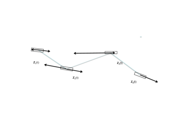
Figure 3: The (approximate) forces acting on the 2-D swimmer from Figure 2 in the fluid.

Assume that

$$S(0)=S_{0}=\{(x=(x_{1},x_{2})\mid-p<x_{1}<p,\;-q<x_{2}<q\},$$ (77)

where $p$ and $q$ are “small” positive numbers.

Theorem 8 (cited from [7] and [9] (Ch. 13))

Let $b=(b_{1},b_{2})$ be a given 2-$D$ vector and $S(0)=S_{0}$ as in (77) lie in $\Omega$. Let $q,p,q^{1-a}/p\rightarrow 0+$ for some $a\in(0,1)$. Then

$$\frac{1}{{\rm mes}\,\{S(0)\}}\mathop{\int}_{S(0)}(Pb\xi)(x)dx\;=\;(b_{1},0)\;+\;O(q^{a})\;+\;O(q^{1-a}/p)\;+\;O(p)$$ (78)

as $q,p,q^{1-a}/p\rightarrow 0+$, where $\xi(x)$ is the characteristic function of $S(0)$.

We can interpret this theorem as that the average projection of a force $b=(b_{1},b_{2})$, acting on a small narrow rectangle, in the fluid velocity space is approximately equal to its projection on the direction parallel to the longer side of the rectangle.

Figure 3 shows the transformation of internal forces of the swimmer from Figure 2 into the forces which actually interact with surrounding medium when the swimmer is in the fluid.

Theorem 9 (cited from [7] and [9] (Ch. 13))

Let $b=(b_{1},b_{2})$ be a given 2-$D$ vector and $S(0)=S_{0}$ be a disc of radius $r$ lying in $\Omega$. Then

$$\frac{1}{{\rm mes}\,\{S(0)\}}\mathop{\int}_{S(0)}(Pb\xi)(x)dx\;=\;\frac{1}{2}(b_{1},b_{2})\;+\;O(r)$$ (79)

as $\;r\rightarrow 0+$, where $\xi(x)$ is the characteristic function of $S(0)$.

We can interpret this theorem as that the average projection of a force $b=(b_{1},b_{2})$, acting on a small disc in the fluid velocity space, is approximately equal to its half.

Lemma 6.1 (cited from [7] and [9] (Ch. 13))

Let $b=(b_{1},b_{2})$ be a given 2-$D$ vector. Let $S(0)\subset\Omega$ be a nonzero measure set which is strictly separated from $\partial\Omega$ and lies in an $r$-neighborhood ($r>0$) of the origin. Then for any subset $Q$ of $\Omega$ of positive measure of diameter $2r$ (that is, it fits some ball of radius $r$) which lies outside of some, say, $d$-neighborhood ($d>0$) of $S(0)$ and is strictly separated from $\partial\Omega$ we have:

$$\frac{1}{{\rm mes}\,\{Q\}}\mathop{\int}_{Q}(Pb\xi)(x)dx\;=\;O(r)$$

as $r\rightarrow 0+$, where $\xi(x)$ is the characteristic function of $S(0)$.

Remark 6.1 (Influence of “remote body forces”)

We can interpret Lemma 6.1 as that the effect of the force $b\xi(x)$ on similar sized sets outside of its support $S(0)$ is “small” if the size of $S(0)$ is “small”. In other words, the results of actions of swimmer’s internal forces applied not directly to the body part at hand are “negligible” relative to the result of the forces applied directly on this body part.

We will use the above-cited results to illustrate possible applications of Theorems 4 and 5 as presented on Figures 3-7.

Examples 6.1: Local controllability of the center of mass/self-propulsion. Consider the swimmer from Figures 1-3 and assume that the rectangles forming its body are asymptotically small and satisfy the assumptions of Theorem 8, and are oriented as on Figure 4-5. Then it follows from Theorem 5 that the swimmer on Figures 4-5 is locally controllable near its center of mass by varying various pairs of $(v_{l},v_{k})$ as long as condition (20) holds.

For example, one can activate only the pair of controls $(v_{3},v_{5})$ in (7) defining the elastic forces acting between $z_{1}(t)$ and $z_{2}(t)$ and between $z_{3}(t)$ and $z_{4}(t)$, see Figures 4 and 5. In this case the 1st pair of internal forces will result in an averaged projected force acting on rectangle $z_{1}(t)$ approximately parallel to its longer side (the elastic force acting on $z_{2}(t)$ can be “neglected” as perpendicular to the longer side of this rectangle). In turn, the 2nd pair of internal forces will create a pair of averaged projected force acting on $z_{3}(t)$ and $z_{4}(t)$ defined by respective spatial orientations of these rectangles. The sum of these forces is not co-linear (under our assumptions) to the averaged projected force acting on $z_{1}(t)$, see Figure 5. Thus, condition (20) holds. In this example the swimmer is capable of local self-propulsion (locomotion) - moving of its center of mass under the actions of its internal forces.

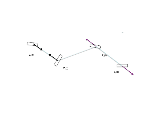
Figure 4: The 2-D swimmer from Figure 2 with 2 pairs of elastic forces acting.

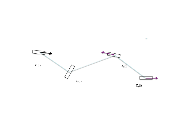
Figure 5: The 2-D swimmer from Figure 4 in the fluid. Approximate averaged projected forces on the fluid velocity space are shown.

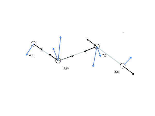
Figure 6: 2-D swimmer consisting of 4 discs.

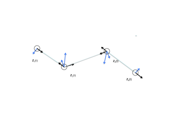
Figure 7: 2-D swimmer from Figure 6 in the fluid. Approximate averaged projection forces on the fluid velocity space are shown.

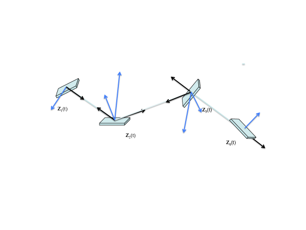
Figure 8: 3-D swimmer consisting of 4 parallelepipeds.

Remark on global controllability in Example 6.1. The local controllability of the center of mass of the swimmer in Example 6.1 means that it can move its center of mass within some neighborhood in any direction by varying controls $(v_{3},v_{5})$ in (7). It does not mean that all points $z_{i}(t)$ will move in the same direction. For example, in the case of shown on Figure 5 $z_{1}$ and $z_{3}$ will (approximately) move to the right, $z_{3}$ will move to the left, while $z_{2}$ will not move. A way to achieve the global swimming controllability of swimmer in Example 6.2 - as a principal possibility to move the center of swimmer’s mass between any two points in $\Omega$ - can be a combination of subsequent employment of various pairs of controls $v_{i}$s which would move the swimmer in small increments towards the target point, while preserving its prescribed structure (such as maintaining allowed limits for deviations of distances between points $z_{i}$’s). This method was applied in [9], Ch. 15 for a 2-$d$ swimmer whose body consisted of three rectangles and for the fluid described by the nonstationary Stokes equations (see also [11] for the 3-$D$ case).

Examples 6.2: On lack of self-propulsion in the case when the swimmer is formed by a set of discs. On Figures 6 and 7 we have the same configuration of a swimmer with the same internal forces but composed of small identical discs. Theorem 9 implies that in this case Theorem 5 does not guarantee the self-propulsion of the swimmer, because the sum of all its averaged projected forces on the fluid velocity space (responsible for the motion of the center of its mass) will remain zero at all times. Namely, these forces will preserve the directions of the original internal forces, while their magnitudes will be reduced by the same factor. In particular, both vectors in condition (20) become zero-vectors. However, we can have the local swimmer’s controllability near all points $z_{i},i=1,2,3,4$, due to Theorem 4.

The center of swimmer’s mass can, in general, also change its location in this example under certain circumstances, for example:

• due to fluid’s drifting motion (such as its natural “flow” associated with given $u_{0}$) or

• due to fluid’s turbulence, induced by the movements of swimmer’s body parts inflicted by actions of its internal forces.

3-$D$ examples. Based on the results of [10], extending Theorems 8 and 9 to the 3-$D$ case, Examples 6.1-2 can be modified as follows:

• Relation analogous to (79) holds in 3-$D$ incompressible fluids with factor 1/3 when the discs are replaced by asymptotically small spheres or cubes, see [10]. Respectively, Example 6.2 will remain unchanged in the case when the body of a 3-$D$ swimmer consists of any finite number of identical spheres or cubes.

• The results as in Example 6.1 can be obtained in the 3-$D$ case for a swimmer whose body consists of parallelepipeds (see Figure 8) whose proportions satisfy certain asymptotic assumptions qualitatively similar to those in Theorem 8, see [10] and illustrating examples in [11].

References

[1]F. Alouges, A. DeSimone, and A. Lefebvre, Optimal
Strokes for Low Reynolds Number Swimmers: An Example, J.
Nonlinear Sci., (2008) 18: 27-302.
[2] H. Brezis, Functional analysis, Sobolev spaces and partial differential equations. Universitext Springer, New York, 2011.
[3] S. Childress, Mechanics of swimming and flying, Cambridge University Press, 1981.
[4] L. J. Fauci & C. S. Peskin, A computational modelof aquatic animal locomotion, J. Comp. Physics 77 (1988), pp. 85–108.
[5] L. J. Fauci, Computational modeling of the swimmingof biflagellated algal cells, Contemporary Mathematics 141 (1993),pp. 91–102.
[6] A. Y. Khapalov, The well-posedness of a model of an
apparatus swimming in the 2-D Stokes fluid, preprint (available as Techn. Rep. 2005-5, Washington State University, Department of Mathematics, http://www.math.wsu.edu/TRS/2005-5.pdf ).
[7]
A.Y. Khapalov, Local controllability for a swimming model, SIAM J. Control. Optim., 46 (2007), pp. 655-682.
[8] A. Y. Khapalov & S. Eubanks, The wellposedness of a 2-D swimming model governed in the nonstationary Stokes fluid by multiplicative controls, Applicable Analysis 88 (2009), pp. 1763–1783.
[9] A. Y. Khapalov, Controllability of partial differential equations governed by multiplicative controls. Lecture Notes in Mathematics Springer, Heidelberg, 2010.
[10] A. Y. Khapalov & G. Trinh, Geometric aspects of transformations of forces acting upon a swimmer in a 3-D incompressible fluid, Disc. Cont. Dyn. Sys. A 33 (2012), no. 4, pp. 1513–1544.
[11] A. Y. Khapalov, Micro motions of a swimmer in the 3-D incompressible fluid governed by the nonstationary Stokes equation, SIAM J. Math. Analysis 45 (2013), no. 6, pp. 3360–3381.
[12] A. Y. Khapalov, Wellposedness of a swimming model in the 3-D incompressible fluid governed by the nonstationary Stokes equation, Int. J. Appl. Math. Comp. Sci. 23 (2013), no. 2, pp. 277–290.
[13] A. Y. Khapalov, P. Cannarsa, F. Priuly and G. Floridia,
Well-posedness of 2-D and 3-D swimming models in incompressible fluids governed by Navier–Stokes equations,
Journal of Mathematical Analysis and Applications 429 (2015), pp. 1059-1085. DOI : 10.1016/j.jmaa.2015.04.044.
[14]J. Koiller, F. Ehlers, and R. Montgomery, Problems
and progress in microswimming, J. Nonlinear Sci., (1996)
6: 507-541.
[15] O. H. Ladyzhenskaya, Mathematical questions of the dynamics of the viscous incompressible fluid, Nauka, Moscow, 1970.
[16] O. H. Ladyzhenskaya, The mathematical theory of viscous incompressible flow, Cordon and Breach, New-York, 1969.
[17]
O.H. Ladyzhenskaya, V.A. Solonikov and N.N. Ural’ceva,
“Linear and Quasi-linear Equations of Parabolic Type,” AMS,
Providence, Rhode Island, 1968.
[18] M. J. Lighthill, Mathematics of biofluiddynamics,
Society for Industrial and Applied Mathematics, Philadelphia, 1975.
[19]K.A. McIsaac and J.P. Ostrowski, Motion planning
for dynamic eel-like robots, Proc. IEEE Int. Conf. Robotics and Automation,
San Francisco, 2000, pp. 1695-1700.
[20]S. Martinez and J. Cort’es, Geometric control
of robotic locomotion systems, Proc. X Fall Workshop on Geometry and
Physics, Madrid, 2001, Publ. de la RSME, Vol. 4 (2001), pp. 183-198.
[21] C. S. Peskin, Numerical analysis of blood
flow in the heart, J. Comp. Physics 25 (1977), pp. 220–252.
[22] C. S. Peskin & D. M. McQueen, A general method
for the computer simulation of biological systems interacting with
fluids, in SEB Symposium on biological fluid dynamics, Leeds, England,
July 5–8, 1994.
[23] M. Sigalotti and J.-C. Vivalda, Controllability properties of a class of systems modeling swimming microscopic organisms, ESAIM: COCV, DOI: 10.1051/cocv/2009034, Published online August 11, 2009.
[24] G. I. Taylor, Analysis of the swimming of
microscopic organisms, Proc. R. Soc. Lond. A 209 (1951), pp .447–461.
[25] G. I. Taylor, Analysis of the swimming of long and
narrow animals, Proc. R. Soc. Lond. A 214 (1952), pp. 158–183.
[26] R. Temam, Navier–Stokes equations. Theory and numerical analysis. 2nd Edition, Studies in Mathematics and its Applications North–Holland, Amsterdam, 1979.
[27]M.S. Trintafyllou, G.S. Trintafyllou and D.K.P. Yue,
Hydrodynamics of fishlike swimming, Ann. Rev. Fluid Mech.,
32 (2000), pp. 33-53.