A decidable weakening of Compass Logic
based on cone-shaped cardinal directions

Abstract.

We introduce a modal logic, called Cone Logic, whose formulas describe properties of points in the plane and spatial relationships between them. Points are labelled by proposition letters and spatial relations are induced by the four cone-shaped cardinal directions. Cone Logic can be seen as a weakening of Venema’s Compass Logic. We prove that, unlike Compass Logic and other projection-based spatial logics, its satisfiability problem is decidable (precisely, PSpace-complete). We also show that it is expressive enough to capture meaningful interval temporal logics – in particular, the interval temporal logic of Allen’s relations ‘Begins’, ‘During’, and ‘Later’, and their transposes.

1. Introduction

Spatial reasoning has both a strong theoretical relevance and many applications in various areas of computer science, including robotics, natural language processing, and geographical information systems [1, 27, 10]. However, despite the widespread interest in the topic, few techniques have been developed to automatically (and efficiently) reason about spatial relations over infinite structures. As a matter of fact, spatial reasoning has been mainly investigated in quite restricted algebraic settings.

Most logical formalisms for spatial reasoning can be conveniently classified into two classes, on the basis of the type of relations they make use of. On the one side, there are logics whose modalities are based on cardinal directions. The most notable example of a formalism in this class is Venema’s Compass Logic [28], which allows one to express properties such as: “from every point labelled with $a$ there is a point to the north of it, that is, above it and vertically aligned to it, that is labelled with $b$”. On the other side, there are formalisms based on topological relations, like the Region Connection Calculus [23, 8], which can express properties such as: “two regions of points, labelled with $a$ and $b$ respectively, are externally connected, that is, tangent”. A quite extensive discussion of the expressiveness of various spatial logics and of their connections can be found in [14].

In this paper, we introduce a novel spatial modal logic, called Cone Logic, which allows one to reason about directional relations between points in the rational plane. Being based on cardinal directions, our logic falls inside the first group of formalisms discussed above. However, unlike most logics based on cardinal directions, the modal operators of Cone Logic range over cone-shaped regions of the plane – formally, over quadrants – rather than semi-axes. To stress this difference, we will often talk of cone-shaped cardinal directions, as opposed to projection-based cardinal directions (see Figure 1). This difference is also reflected in considerably better algorithmic properties. While the satisfiability problem for modal logics with projection-based cardinal directions – notably, Compass Logic – turns out to be highly undecidable [17, 20], we prove that Cone Logic enjoys a decidable satisfiability problem (in fact, PSpace-complete) by making use of a suitable filtration technique. We also show that Cone Logic subsumes interesting interval temporal logics such as the temporal logic of sub-intervals/super-intervals, thus generalizing previous results in the literature [6] and basically disproving a conjecture by Lodaya [12].

Related work. The paper that is most related in spirit to the present work is that of Venema [28], who studies Compass Logic. Compass Logic is a two-dimensional modal logic interpreted over the Cartesian product of two linear orders, which features two pairs of modalities, each pair ranging over one of the two orders. The first undecidability result for the satisfiability problem of Compass Logic was shown in [17] and it covers both the case where the logic is interpreted over the discrete infinite grid $\mathbb{N}\times\mathbb{N}$ and the case where the logic is interpreted over the Euclidean space $\mathbb{R}\times\mathbb{R}$. In [24], similar formalisms based on products of two linear modal logics have been studied and the above-mentioned undecidability results have been strengthened to cover practically all classes of products of infinite/unbounded linear orders. These negative results stem from the possibility of encoding halting computations of Turing machines inside a two-dimensional structure and expressing the correctness of the encoding in the logic.

Cone Logic can be viewed as the fragment of Venema’s Compass Logic obtained from the full logic by enforcing the following restriction: quantifications along one axis can be used only after a similar quantification along the other axis. Such a constrain makes it impossible to correctly encode computations of Turing machines in the underlying two-dimensional space, thus leaving room to recover the decidability of the satisfiability problem.

There is also a tight connection between modal logics over two-dimensional spaces and fragments of Halpern and Shoham’s modal logic of time intervals (HS) [11]. According to such a correspondence, intervals over a linearly ordered temporal domain are interpreted as points over a two-dimensional space. In Section 7, we will show how such a correspondence can be lifted to the logical level, by reducing the satisfiability problem for an expressive fragment of HS to the satisfiability problem for (a subset of formulas of) Cone Logic.

Other multi-dimensional spatial logics are studied in [25, 3, 4] (with different goals in mind). Some of them retain good decidability properties, but their expressive power is often limited. An example is the logic proposed by Bennett in [3], which uses a single modal operator interpreted as the interior in a given topology. This logic is essentially equivalent to S4 and its satisfiability problem is PSpace-complete.

Structure of the paper. In Section 2, we define syntax and semantics of Cone Logic and we discuss its expressiveness and satisfiability problem. In Section 3, we introduce the basic machinery for attacking the satisfiability problem. In Section 4, we show how to turn a labelled region of the rational plane into an infinite (decomposition) tree structure. Then, in Section 5, we prove a tree (pseudo-)model property for Cone Logic, that is, we describe models of satisfiable Cone Logic formulas by means of suitable labelled tree structures. In Section 6, we exploit such a tree model property to reduce the satisfiability problem for Cone Logic to the satisfiability problem for a simple fragment of CTL. In Section 7, we make use of such a decidability result to prove that a meaningful fragment of Halpern and Shoham’s interval temporal logic HS, interpreted over dense linear structures, is decidable in polynomial space. In Section 8, we make some final remarks and we discuss related and open problems.

2. The logic

In this paper, we generically denote by $\mathbb{P}$ either the rational plane $\mathbb{Q}\times\mathbb{Q}$ or the real (Euclidean) plane $\mathbb{R}\times\mathbb{R}$. We will define the semantics of formulas of Cone Logic in the same way over labellings of the rational plane and labellings of the real plane.

We call spatial relation any binary relation $\,\mathbin{\ooalign{\raisebox{-2.2pt}{\includegraphics{figures/symbols.49}}\crcr\scriptsize$\mspace{-3.0mu}d$}}\,\in\mathbb{P}\times\mathbb{P}$ between points in the plane. We use the infix notation $p\,\mathbin{\ooalign{\raisebox{-2.2pt}{\includegraphics{figures/symbols.49}}\crcr\scriptsize$\mspace{-3.0mu}d$}}\,q$ for saying that two points $p,q\in\mathbb{P}$ satisfy a given spatial relation $\,\mathbin{\ooalign{\raisebox{-2.2pt}{\includegraphics{figures/symbols.49}}\crcr\scriptsize$\mspace{-3.0mu}d$}}\,$. We start by defining some basic spatial relations, denoted   ,   ,   ,   , that correspond to the four projection-based cardinal directions ‘North’, ‘South’, ‘East’ and ‘West’ (see Figure 1 - left):

$$\begin{array}[]{rclrcl}(x,y)~{}\,\raisebox{-2.2pt}{\includegraphics{figures/symbols.50}}\,~{}(x^{\prime},y^{\prime})&~{}\text{iff}&~{}x=x^{\prime}\wedge y<y^{\prime}&\quad\quad(x,y)~{}\,\raisebox{-2.2pt}{\includegraphics{figures/symbols.51}}\,~{}(x^{\prime},y^{\prime})&~{}\text{iff}&~{}x=x^{\prime}\wedge y>y^{\prime}\\[8.61108pt] (x,y)~{}\,\raisebox{-2.2pt}{\includegraphics{figures/symbols.52}}\,~{}(x^{\prime},y^{\prime})&~{}\text{iff}&~{}x<x^{\prime}\wedge y=y^{\prime}&\quad\quad(x,y)~{}\,\raisebox{-2.2pt}{\includegraphics{figures/symbols.53}}\,~{}(x^{\prime},y^{\prime})&~{}\text{iff}&~{}x>x^{\prime}\wedge y=y^{\prime}.\end{array}$$

Using the above basic relations and set-theoretic operations, one can construct new spatial relations. We define the composition of two spatial relations $\,\mathbin{\ooalign{\raisebox{-2.2pt}{\includegraphics{figures/symbols.49}}\crcr\scriptsize$\mspace{-3.0mu}d$}}\,$ and $\,\mathbin{\ooalign{\raisebox{-2.2pt}{\includegraphics{figures/symbols.49}}\crcr\scriptsize$\mspace{-3.0mu}e$}}\,$ by $\,\mathbin{\ooalign{\raisebox{-2.2pt}{\includegraphics{figures/symbols.49}}\crcr\scriptsize$\mspace{-3.0mu}d$}}\,\,\mathbin{\ooalign{\raisebox{-2.2pt}{\includegraphics{figures/symbols.49}}\crcr\scriptsize$\mspace{-3.0mu}e$}}\,={\bigl{\{}(p,r)\,:\,\exists{\;q\in\mathbb{P}}.\;~{}(p,q)\in\,\mathbin{\ooalign{\raisebox{-2.2pt}{\includegraphics{figures/symbols.49}}\crcr\scriptsize$\mspace{-3.0mu}d$}}\,\wedge(q,r)\in\,\mathbin{\ooalign{\raisebox{-2.2pt}{\includegraphics{figures/symbols.49}}\crcr\scriptsize$\mspace{-3.0mu}e$}}\,\bigr{\}}}$. We are interested in the following spatial relations:

$$\begin{array}[]{rclrcl}\,\raisebox{-2.2pt}{\includegraphics{figures/symbols.41}}&~{}=&~{}\,\raisebox{-2.2pt}{\includegraphics{figures/symbols.50}}\,\,\raisebox{-2.2pt}{\includegraphics{figures/symbols.53}}\,\cup\,\raisebox{-2.2pt}{\includegraphics{figures/symbols.53}}&\qquad\qquad\qquad\,\raisebox{-2.2pt}{\includegraphics{figures/symbols.40}}&~{}=&~{}\,\raisebox{-2.2pt}{\includegraphics{figures/symbols.50}}\,\,\raisebox{-2.2pt}{\includegraphics{figures/symbols.52}}\,\cup\,\raisebox{-2.2pt}{\includegraphics{figures/symbols.52}}\\[8.61108pt] \,\raisebox{-2.2pt}{\includegraphics{figures/symbols.43}}&~{}=&~{}\,\raisebox{-2.2pt}{\includegraphics{figures/symbols.51}}\,\,\raisebox{-2.2pt}{\includegraphics{figures/symbols.53}}\,\cup\,\raisebox{-2.2pt}{\includegraphics{figures/symbols.53}}&\qquad\qquad\qquad\,\raisebox{-2.2pt}{\includegraphics{figures/symbols.42}}&~{}=&~{}\,\raisebox{-2.2pt}{\includegraphics{figures/symbols.51}}\,\,\raisebox{-2.2pt}{\includegraphics{figures/symbols.52}}\,\cup\,\raisebox{-2.2pt}{\includegraphics{figures/symbols.52}}\end{array}$$

Observe that, up to a rotation of the axes, the derived relations $\,\raisebox{-2.2pt}{\includegraphics{figures/symbols.37}}\,=\,\raisebox{-2.2pt}{\includegraphics{figures/symbols.50}}\,\,\raisebox{-2.2pt}{\includegraphics{figures/symbols.41}}\,$, $\,\raisebox{-2.2pt}{\includegraphics{figures/symbols.36}}\,=\,\raisebox{-2.2pt}{\includegraphics{figures/symbols.50}}\,\,\raisebox{-2.2pt}{\includegraphics{figures/symbols.40}}\,$, $\,\raisebox{-2.2pt}{\includegraphics{figures/symbols.39}}\,=\,\raisebox{-2.2pt}{\includegraphics{figures/symbols.51}}\,\,\raisebox{-2.2pt}{\includegraphics{figures/symbols.43}}\,$, and $\,\raisebox{-2.2pt}{\includegraphics{figures/symbols.38}}\,=\,\raisebox{-2.2pt}{\includegraphics{figures/symbols.51}}\,\,\raisebox{-2.2pt}{\includegraphics{figures/symbols.42}}\,$ can be viewed as the four cone-shaped cardinal relations ‘North’, ‘East’, ‘West’ and ‘South’ [9] (see Figure 1 - right).

Figure 1. Projection-based and cone-shaped cardinal directions.

We introduce Cone Logic as a modal logic based on specific spatial relations. As such, it can express properties of single elements (the labels associated with the points in a plane) and binary relationships between elements (it admits existential quantifications over points that satisfy a given spatial relation). The modal operators of Cone Logic are induced by the six spatial relations   ,   ,   ,   ,   ,    (the reason for such a choice will become evident in the following). Unless otherwise specified, hereafter the term “spatial relation” will always refer to one of these six relations.

Given a set $\Sigma$ of proposition letters, formulas of Cone Logic are built up from $\Sigma$ using the Boolean connectives and and the existential modalities that correspond to the six spatial relations:

$$\varphi \>\>\>:=\>\>\>a \forall a\in\Sigma$$ ()

$$\>\>\>\>\>\>\>||\>\>\>\neg\varphi^{\prime}\>\>\>||\>\>\>\varphi^{\prime}\vee\varphi^{\prime\prime}$$

$$\>\>\>\>\>\>\>||\>\>\>\!\!\,\mathbin{\ooalign{\raisebox{-2.7pt}{\includegraphics{figures/symbols.31}}\crcr\scriptsize$\mspace{-5.0mu}d$}}\varphi^{\prime}\qquad\qquad$$

We evaluate Cone Logic formulas over labellings of the plane or (sub)regions of it, starting from an initial point. Precisely, our models are structures of the form ${\langle P,(R_{a})_{a\in\Sigma},p\rangle}$, where $P\subseteq\mathbb{P}$, $R_{a}\subseteq P$ for all $a\in\Sigma$, and $p\in P$. The formal semantics is defined as follows:

• for all proposition letters $a\in\Sigma$, ${\langle P,(R_{a})_{a\in\Sigma},p\rangle}\vDash a$ iff $p\in R_{a}$,

• ${\langle P,(R_{a})_{a\in\Sigma},p\rangle}\vDash\neg\varphi^{\prime}$ iff ${\langle P,(R_{a})_{\Sigma},p\rangle}\mathrel{\mathchoice{\ooalign{$\hfil\displaystyle/\hfil$\crcr$\displaystyle\vDash$}}{\ooalign{$\hfil\textstyle/\hfil$\crcr$\textstyle\vDash$}}{\ooalign{$\hfil\scriptstyle/\hfil$\crcr$\scriptstyle\vDash$}}{\ooalign{$\hfil\scriptscriptstyle/\hfil$\crcr$\scriptscriptstyle\vDash$}}}\varphi^{\prime}$,

• ${\langle P,(R_{a})_{a\in\Sigma},p\rangle}\vDash\varphi^{\prime}\vee\varphi^{\prime\prime}$ iff ${\langle P,(R_{a})_{a\in\Sigma},p\rangle}\vDash\varphi^{\prime}$ or ${\langle P,(R_{a})_{a\in\Sigma},p\rangle}\vDash\varphi^{\prime\prime}$,

• for all spatial relations $\,\mathbin{\ooalign{\raisebox{-2.2pt}{\includegraphics{figures/symbols.49}}\crcr\scriptsize$\mspace{-3.0mu}d$}}\,$, ${\langle P,(R_{a})_{a\in\Sigma},p\rangle}\vDash\,\mathbin{\ooalign{\raisebox{-2.7pt}{\includegraphics{figures/symbols.31}}\crcr\scriptsize$\mspace{-5.0mu}d$}}\varphi^{\prime}$ iff ${\langle P,(R_{a})_{a\in\Sigma},q\rangle}\vDash\varphi^{\prime}$ for some point $q\in P$ such that $p\,\mathbin{\ooalign{\raisebox{-2.2pt}{\includegraphics{figures/symbols.49}}\crcr\scriptsize$\mspace{-3.0mu}d$}}\,q$.

We will freely use shorthands like $\varphi^{\prime}\wedge\varphi^{\prime\prime}=\neg(\neg\varphi^{\prime}\vee\neg\varphi^{\prime\prime})$, $\bot=a\wedge\neg a$, $\,\raisebox{-2.7pt}{\includegraphics{figures/symbols.19}}\varphi=\,\raisebox{-2.7pt}{\includegraphics{figures/symbols.32}}\,\raisebox{-2.7pt}{\includegraphics{figures/symbols.23}}\varphi$, $\,\mspace{1.7mu}\raisebox{-1.6pt}{\includegraphics{figures/symbols.1}}\mspace{1.7mu}\varphi=\neg\,\raisebox{-2.7pt}{\includegraphics{figures/symbols.19}}\neg\varphi$, $\,\mspace{1.7mu}\raisebox{-1.6pt}{\includegraphics{figures/symbols.8}}\mspace{1.7mu}\varphi=\,\mspace{1.7mu}\raisebox{-1.6pt}{\includegraphics{figures/symbols.1}}\mspace{1.7mu}\,\mspace{1.7mu}\raisebox{-1.6pt}{\includegraphics{figures/symbols.0}}\mspace{1.7mu}\varphi$, $\,\mspace{1.7mu}\raisebox{-1.6pt}{\includegraphics{figures/symbols.12}}\mspace{1.7mu}\varphi=\,\mspace{1.7mu}\raisebox{-1.6pt}{\includegraphics{figures/symbols.1}}\mspace{1.7mu}\,\mspace{1.7mu}\raisebox{-1.6pt}{\includegraphics{figures/symbols.2}}\mspace{1.7mu}\varphi$, and so on.

Cone Logic is well-suited for expressing spatial relationships between points, curves, and regions over the plane. Below, we give an intuitive account of its expressiveness through a couple of examples.

To begin with, we show how to define an $a$-labelled open rectangular region, whose edges are aligned with the $x$- and $y$-axes (see Figure 2):

$$\begin{array}[]{rcl}\varphi&~{}=&~{}\,\raisebox{-2.7pt}{\includegraphics{figures/symbols.30}}a\wedge\,\raisebox{-2.7pt}{\includegraphics{figures/symbols.30}}b\wedge\,\raisebox{-2.7pt}{\includegraphics{figures/symbols.30}}c\wedge\,\raisebox{-2.7pt}{\includegraphics{figures/symbols.30}}d\wedge\,\raisebox{-2.7pt}{\includegraphics{figures/symbols.30}}e\\[4.30554pt] &\wedge{}\hfil&~{}\,\mspace{1.7mu}\raisebox{-1.6pt}{\includegraphics{figures/symbols.12}}\mspace{1.7mu}(a\rightarrow\,\raisebox{-2.7pt}{\includegraphics{figures/symbols.18}}a\wedge\,\raisebox{-2.7pt}{\includegraphics{figures/symbols.21}}a)\wedge\,\mspace{1.7mu}\raisebox{-1.6pt}{\includegraphics{figures/symbols.12}}\mspace{1.7mu}(\neg a\leftrightarrow b\!\vee\!c\!\vee\!d\!\vee\!e)\\[4.30554pt] &\wedge{}\hfil&~{}\,\mspace{1.7mu}\raisebox{-1.6pt}{\includegraphics{figures/symbols.12}}\mspace{1.7mu}(b\rightarrow\,\mspace{1.7mu}\raisebox{-1.6pt}{\includegraphics{figures/symbols.11}}\mspace{1.7mu}b)\wedge\,\mspace{1.7mu}\raisebox{-1.6pt}{\includegraphics{figures/symbols.12}}\mspace{1.7mu}(c\rightarrow\,\mspace{1.7mu}\raisebox{-1.6pt}{\includegraphics{figures/symbols.10}}\mspace{1.7mu}c)\wedge\,\mspace{1.7mu}\raisebox{-1.6pt}{\includegraphics{figures/symbols.12}}\mspace{1.7mu}(d\rightarrow\,\mspace{1.7mu}\raisebox{-1.6pt}{\includegraphics{figures/symbols.9}}\mspace{1.7mu}d)\wedge\,\mspace{1.7mu}\raisebox{-1.6pt}{\includegraphics{figures/symbols.12}}\mspace{1.7mu}(e\rightarrow\,\mspace{1.7mu}\raisebox{-1.6pt}{\includegraphics{figures/symbols.8}}\mspace{1.7mu}e).\end{array}$$

Figure 2. An $a$-labelled open rectangle.

The second example uses the derived operators   and   to enforce non-trivial spatial relationships between labelled regions of the rational plane. Let $\Sigma$ be an alphabet containing $n+2$ proposition letters $a,b_{1},...,b_{n},c$ and let $<$ be the partial order over $\Sigma$ such that $a<b_{i}<c$, for all $1\le i\le n$, and $b_{i}\mathrel{\mathchoice{\ooalign{$\hfil\displaystyle/\hfil$\crcr$\displaystyle<$}}{\ooalign{$\hfil\textstyle/\hfil$\crcr$\textstyle<$}}{\ooalign{$\hfil\scriptstyle/\hfil$\crcr$\scriptstyle<$}}{\ooalign{$\hfil\scriptscriptstyle/\hfil$\crcr$\scriptscriptstyle<$}}}b_{j}$, for all $1\le i,j\le n$ with $i\neq j$. As usual, we write $a\le b$ (resp., $a\ge b$) if $a=b$ or $a<b$ (resp., $a>b$). Consider now the formula $\varphi$ defined as follows:

$$\begin{array}[]{rcl}\varphi&=&\,\mspace{1.7mu}\raisebox{-1.6pt}{\includegraphics{figures/symbols.12}}\mspace{1.7mu}\!\displaystyle\tbigvee\slimits@\limits_{d\in\Sigma}\!d~{}~{}\wedge~{}~{}\,\mspace{1.7mu}\raisebox{-1.6pt}{\includegraphics{figures/symbols.12}}\mspace{1.7mu}\!\displaystyle\tbigwedge\slimits@\limits_{d\neq e}\!\neg(d\wedge e)~{}\wedge~{}\,\mspace{1.7mu}\raisebox{-1.6pt}{\includegraphics{figures/symbols.12}}\mspace{1.7mu}\!\displaystyle\tbigwedge\slimits@\limits_{d\in\Sigma}\Bigl{(}d~{}\rightarrow~{}\displaystyle\tbigwedge\slimits@\limits_{e\ge d}\!\!\,\raisebox{-2.7pt}{\includegraphics{figures/symbols.18}}e~{}\wedge\,\mspace{1.7mu}\raisebox{-1.6pt}{\includegraphics{figures/symbols.0}}\mspace{1.7mu}\!\tbigvee\slimits@\limits_{e\ge d}\!e~{}\wedge\displaystyle\tbigwedge\slimits@\limits_{e\le d}\!\!\,\raisebox{-2.7pt}{\includegraphics{figures/symbols.21}}e~{}\wedge\,\mspace{1.7mu}\raisebox{-1.6pt}{\includegraphics{figures/symbols.3}}\mspace{1.7mu}\!\tbigvee\slimits@\limits_{e\le d}\!e\Bigr{)}\ .\end{array}$$

The unique (up to homomorphism) labelling of the rational plane $\mathbb{Q}\times\mathbb{Q}$ that satisfies $\varphi$ is depicted in Figure 3. Notice that each $b_{i}$-labelled region is an infinite union of disjoint open rectangles (the coordinates of their corners are given by pairs of irrational numbers, which, of course, do not belong to the rational plane). Moreover, the $b_{i}$-labelled open rectangles are arranged densely in the rational plane, that is, for all $1\le i,j,k\le n$, with $i\neq j$, all $b_{i}$-labelled points $(x_{i},y_{i})$, and all $b_{j}$-labelled points $(x_{j},y_{j}$), with $x_{i}<x_{j}$ and $y_{i}>y_{j}$, there is a $b_{k}$-labelled point $(x_{k},y_{k})$ such that $x_{1}<x_{k}<x_{2}$ and $y_{1}>y_{k}>y_{2}$. We also observe that the formula $\varphi$ cannot be satisfied by any labelling of the real plane $\mathbb{R}\times\mathbb{R}$. Indeed, $\varphi$ requires that the subregions $R_{a},R_{b_{1}},...,R_{b_{n}},R_{c}$ are “open” (in the sense that they do not contain points on their boundaries) and they form a partition of the plane: this is against the assumption that the plane is compact, as in this case boundaries would be covered by the subregions.

Figure 3. A labelled rational plane satisfying $\varphi$.

In the following, we focus our attention on the satisfiability problem for Cone Logic, which consists of deciding whether a given formula $\varphi$ holds at some point of a labelled region of the (rational or real) plane. In particular, we are interested in satisfiability of formulas interpreted over rectangular regions of the form $X\times Y$, where $X$ and $Y$ are open or closed intervals of $\mathbb{Q}$ (resp., $\mathbb{R}$). Before describing our decision procedure for the satisfiability problem for Cone Logic, we make a few remarks.

Remark 1.

In Example 2, we showed that there exist Cone Logic formulas that can only be satisfied over dense non-Euclidean (e.g., rational) planes. Here, we prove that the converse does not hold, namely, that every formula of Cone Logic that is satisfied in some (rational or real) plane is also satisfiable in the rational plane. First of all, we observe that Cone Logic can be viewed as a fragment of classical first-order logic that uses pairs of elements of the underlying domain to denote points, some binary relations to represent their labels, and a (definable) dense linear order to describe the spatial relations. As an example, a Cone Logic formula of the form:

$$\varphi~{}=~{}\,\raisebox{-2.7pt}{\includegraphics{figures/symbols.22}}a$$

can be translated into the following, equi-satisfiable first-order formula:

$$\begin{array}[]{rl}\tilde{\varphi}(x,y)&=~{}\text{\it``\,$<$ is a dense linear order with neither a minimal nor a maximal element''}\\ &\wedge\>\>\>\exists{\;x^{\prime},y^{\prime}}.\;\>\>x<x^{\prime}~{}\wedge~{}(y=y^{\prime}\vee y<y^{\prime})~{}\wedge~{}R_{a}(x^{\prime},y^{\prime}).\end{array}$$

According to the above translation, if $\tilde{\varphi}(x,y)$ holds in some structure ${\langle L,(R_{a})_{a\in\Sigma},<,i,j\rangle}$, where $R_{a}$ and $<$ are binary relations on the domain $L$ and $i,j$ are elements of $L$, then $(L,<)$ is a dense linear order with neither a minimal nor a maximal element and $\varphi$ holds in the labelled plane ${\langle L\times L,(R_{a})_{a\in\Sigma},(i,j)\rangle}$. As $\tilde{\varphi}(x,y)$ is a first-order formula, it follows from Löwenheim-Skolem theorem that, without loss of generality, $L$ can be assumed to be countable. Finally, since $(\mathbb{Q},<)$ is up to isomorphism the only countable dense linear order with neither a minimal nor a maximal element, we conclude that $\varphi$ is satisfied by a labelling of the rational plane.

Remark 2.

Recall that the rational (resp., real) plane is homomorphic to any open rectangular subregion of it of the form $X\times Y$, with $X=(x_{0},x_{1})$ and $Y=(y_{0},y_{1})$ open intervals. This means that, for the purpose of studying satisfiability of Cone Logic, it does not matter if we consider labellings of the entire plane or labellings of open rectangular subregions of it. Similarly, the complexity of the satisfiability problem does not change if we consider closed rectangles. Indeed, any formula $\varphi$ of Cone Logic, interpreted over a region of the form $X\times Y$, where $X=(x_{0},x_{1})$ is an open interval, can be rewritten into an equi-satisfiable formula $\bar{\varphi}$, interpreted over the region $\bar{X}\times Y$, where $\bar{X}=[x_{0},x_{1}]$ is a closed, non-singleton interval, and vice versa. As an example, the Cone Logic formula

$$\varphi~{}=~{}\,\raisebox{-2.7pt}{\includegraphics{figures/symbols.22}}a$$

interpreted over a labelling of $(x_{0},x_{1})\times\mathbb{Q}$ can be rewritten as

$$\bar{\varphi}~{}=~{}\,\mspace{1.7mu}\raisebox{-1.6pt}{\includegraphics{figures/symbols.12}}\mspace{1.7mu}\big{(}\,\mspace{1.7mu}\raisebox{-1.6pt}{\includegraphics{figures/symbols.10}}\mspace{1.7mu}\bot\vee\,\mspace{1.7mu}\raisebox{-1.6pt}{\includegraphics{figures/symbols.11}}\mspace{1.7mu}\bot\rightarrow a\big{)}\wedge\,\raisebox{-2.7pt}{\includegraphics{figures/symbols.22}}a$$

which is interpreted over a labelling of $[x_{0},x_{1}]\times\mathbb{Q}$ (the idea is that points along left and right boundaries are labelled with the fresh proposition letter $a$).

Thanks to the above two remarks, we can restrict our attention to satisfiability of Cone Logic formulas over specific regions of the plane, called stripes.

A stripe is a region of the form $X\times\mathbb{Q}$, where $X=[x_{0},x_{1}]$ is a closed non-singleton interval.

The relationships between the Cone Logic and other two-dimensional modal logics deserve a little discussion. Many logics interpreted over two-dimensional structures make use of projection-based modalities, that is, modalities induced by the accessibility relations along the two orthogonal axes. Compass Logic [28] is the most notable example of these two-dimensional logics, as it comprises the four modalities  ,  ,  ,  , allowing one to move along one of the two coordinates while keeping the other coordinate constant. As we have already seen, modalities based on cone-shaped cardinal directions can be easily defined in terms of projection-based modalities, e.g., $\,\raisebox{-2.7pt}{\includegraphics{figures/symbols.18}}\varphi=\,\raisebox{-2.7pt}{\includegraphics{figures/symbols.32}}\,\raisebox{-2.7pt}{\includegraphics{figures/symbols.34}}\varphi$. Cone Logic can thus be viewed as a fragment of Compass Logic. However, Cone Logic inherits from Compass Logic only some desirable features. For instance, suppose that one is interested in constraining a given proposition letter $a$ to occur along the positive $x$-axis, and possibly somewhere else. Such a condition can be easily forced in Compass Logic by means of the formula $\,\raisebox{-2.7pt}{\includegraphics{figures/symbols.34}}a$. Cone Logic can enforce a similar constraint by means of the formula

$$\,\mspace{1.7mu}\raisebox{-1.6pt}{\includegraphics{figures/symbols.12}}\mspace{1.7mu}(y_{0}\vee\,\raisebox{-2.7pt}{\includegraphics{figures/symbols.32}}y_{0}\vee\,\raisebox{-2.7pt}{\includegraphics{figures/symbols.33}}y_{0})\wedge\,\mspace{1.7mu}\raisebox{-1.6pt}{\includegraphics{figures/symbols.8}}\mspace{1.7mu}\neg y_{0}\wedge\,\mspace{1.7mu}\raisebox{-1.6pt}{\includegraphics{figures/symbols.9}}\mspace{1.7mu}\neg y_{0}\wedge\,\raisebox{-2.7pt}{\includegraphics{figures/symbols.28}}(a\wedge y_{0}),\phantom{\ .~{}}$$

where $y_{0}$ is a fresh proposition letter. Similarly, the Compass Logic formula $\,\mspace{1.7mu}\raisebox{-1.6pt}{\includegraphics{figures/symbols.16}}\mspace{1.7mu}a$ can be expressed in Cone Logic as follows:

$$\,\mspace{1.7mu}\raisebox{-1.6pt}{\includegraphics{figures/symbols.12}}\mspace{1.7mu}(y_{0}\vee\,\raisebox{-2.7pt}{\includegraphics{figures/symbols.32}}y_{0}\vee\,\raisebox{-2.7pt}{\includegraphics{figures/symbols.33}}y_{0})\wedge\,\mspace{1.7mu}\raisebox{-1.6pt}{\includegraphics{figures/symbols.8}}\mspace{1.7mu}\neg y_{0}\wedge\,\mspace{1.7mu}\raisebox{-1.6pt}{\includegraphics{figures/symbols.9}}\mspace{1.7mu}\neg y_{0}\wedge\,\mspace{1.7mu}\raisebox{-1.6pt}{\includegraphics{figures/symbols.10}}\mspace{1.7mu}(y_{0}\rightarrow a).$$

It is worth noticing, however, that the above translations can be performed at the cost of introducing additional labels – e.g., $y_{0}$ – that can only appear along specific axes. Hence, only boundedly many constraints of the above forms can be enforced within a single formula of Cone Logic. We will see that such a limitation (weakening) can be traded for a positive decidability result.

3. Basic machinery: types, dependencies, clusters, and shadings

From now on, we refer to a generic formula $\varphi$ of Cone Logic. The basic idea underlying the decision procedure for the satisfiability of $\varphi$ is to first look at how the spatial constraints defined by the subformulas of $\varphi$ can be satisfied locally over the points of the plane and then to propagate these constraints to larger and larger regions of the plane. Below, we introduce some key concepts that ease such an analysis.

Let $\varphi$ be a formula of Cone Logic. The closure of $\varphi$, denoted by $\mathsf{closure}(\varphi)$, is the set of all subformulas of $\varphi$ and of their negations (we identify any subformula $\neg\neg\alpha$ with $\alpha$). A $\varphi$-atom is a non-empty set $A\subseteq\mathsf{closure}(\varphi)$ such that:

• for every formula $\alpha\in\mathsf{closure}(\varphi)$, $\alpha\in A$ iff $\neg\alpha\mathrel{\mathchoice{\ooalign{$\hfil\displaystyle/\hfil$\crcr$\displaystyle\in$}}{\ooalign{$\hfil\textstyle/\hfil$\crcr$\textstyle\in$}}{\ooalign{$\hfil\scriptstyle/\hfil$\crcr$\scriptstyle\in$}}{\ooalign{$\hfil\scriptscriptstyle/\hfil$\crcr$\scriptscriptstyle\in$}}}A$,

• for every formula $\gamma=\alpha\vee\beta\in\mathsf{closure}(\varphi)$, $\gamma\in A$ iff $\alpha\in A$ or $\beta\in A$.

Note that the cardinality of $\mathsf{closure}(\varphi)$ is linear in the size ${\lvert\varphi\rvert}$ of $\varphi$, while the number of $\varphi$-atoms is at most exponential in ${\lvert\varphi\rvert}$.

Let $\mathcal{P}={\langle P,(R_{a})_{a\in\Sigma}\rangle}$ be a labelled region. We associate with each point $p$ in $P$ the set of all formulas $\alpha\in\mathsf{closure}(\varphi)$ such that ${\langle\mathcal{P},p\rangle}\vDash\alpha$. Such a set is called the $\varphi$-type of $p$ and it is denoted by $\mathsf{type}_{\mathcal{P}}(p)$. It can be easily checked that each $\varphi$-type is a $\varphi$-atom, but not vice versa.

Given a $\varphi$-atom $A$ and a spatial relation $\,\mathbin{\ooalign{\raisebox{-2.2pt}{\includegraphics{figures/symbols.49}}\crcr\scriptsize$\mspace{-3.0mu}d$}}\,$, we denote by $\,\mathbin{\ooalign{\raisebox{-2.7pt}{\includegraphics{figures/symbols.31}}\crcr\scriptsize$\mspace{-5.0mu}d$}}\mathsf{-req}(A)$ the set of all formulas $\alpha\in\mathsf{closure}(\varphi)$ such that $\,\mathbin{\ooalign{\raisebox{-2.7pt}{\includegraphics{figures/symbols.31}}\crcr\scriptsize$\mspace{-5.0mu}d$}}\alpha\in A$.These formulas can be thought of as the requests of $A$ along the direction $\,\mathbin{\ooalign{\raisebox{-2.2pt}{\includegraphics{figures/symbols.49}}\crcr\scriptsize$\mspace{-3.0mu}d$}}\,$. Similarly, we denote by $\,\mathbin{\ooalign{\raisebox{-2.7pt}{\includegraphics{figures/symbols.31}}\crcr\scriptsize$\mspace{-5.0mu}d$}}\mathsf{-obs}(A)$ the set of all formulas $\alpha\in A$ such that $\,\mathbin{\ooalign{\raisebox{-2.7pt}{\includegraphics{figures/symbols.31}}\crcr\scriptsize$\mspace{-5.0mu}d$}}\alpha\in\mathsf{closure}(\varphi)$. These formulas can be thought of as the observables of $A$ along the direction $\,\mathbin{\ooalign{\raisebox{-2.2pt}{\includegraphics{figures/symbols.49}}\crcr\scriptsize$\mspace{-3.0mu}d$}}\,$. Making use of these sets, we can associate with each spatial relation $\,\mathbin{\ooalign{\raisebox{-2.2pt}{\includegraphics{figures/symbols.49}}\crcr\scriptsize$\mspace{-3.0mu}d$}}\,$ a corresponding relation between $\varphi$-atoms (with a little abuse of notation, we denote it by $\,\mathbin{\ooalign{\raisebox{-2.2pt}{\includegraphics{figures/symbols.49}}\crcr\scriptsize$\mspace{-3.0mu}d$}}\,$).

Let $\,\mathbin{\ooalign{\raisebox{-2.2pt}{\includegraphics{figures/symbols.49}}\crcr\scriptsize$\mspace{-3.0mu}d$}}\,\in\big{\{}\,\raisebox{-2.2pt}{\includegraphics{figures/symbols.50}}\,,\,\raisebox{-2.2pt}{\includegraphics{figures/symbols.51}}\,,\,\raisebox{-2.2pt}{\includegraphics{figures/symbols.41}}\,,\,\raisebox{-2.2pt}{\includegraphics{figures/symbols.40}}\,,\,\raisebox{-2.2pt}{\includegraphics{figures/symbols.43}}\,,\,\raisebox{-2.2pt}{\includegraphics{figures/symbols.42}}\,\big{\}}$ be a spatial relation and $A,B$ be two $\varphi$-atoms. We write $A\,\mathbin{\ooalign{\raisebox{-2.2pt}{\includegraphics{figures/symbols.49}}\crcr\scriptsize$\mspace{-3.0mu}d$}}\,B$ if and only if it holds that:

$$\begin{array}[]{lll}\,\mathbin{\ooalign{\raisebox{-2.7pt}{\includegraphics{figures/symbols.31}}\crcr\scriptsize$\mspace{-5.0mu}e$}}\mathsf{-req}(A)&\supseteq{}&~{}\,\mathbin{\ooalign{\raisebox{-2.7pt}{\includegraphics{figures/symbols.31}}\crcr\scriptsize$\mspace{-5.0mu}e$}}\mathsf{-obs}(B)\,\cup\,\mathbin{\ooalign{\raisebox{-2.7pt}{\includegraphics{figures/symbols.31}}\crcr\scriptsize$\mspace{-5.0mu}e$}}\mathsf{-req}(B);\\[4.30554pt] \,\mathbin{\ooalign{\raisebox{-2.7pt}{\includegraphics{figures/symbols.31}}\crcr\scriptsize$\mspace{-5.0mu}e\!^{\prime}$}}\mathsf{-req}(B)&\supseteq{}&~{}\,\mathbin{\ooalign{\raisebox{-2.7pt}{\includegraphics{figures/symbols.31}}\crcr\scriptsize$\mspace{-5.0mu}e\!^{\prime}$}}\mathsf{-obs}(A)\,\cup\,\mathbin{\ooalign{\raisebox{-2.7pt}{\includegraphics{figures/symbols.31}}\crcr\scriptsize$\mspace{-5.0mu}e\!^{\prime}$}}\mathsf{-req}(A),\end{array}$$

for all spatial relations $\,\mathbin{\ooalign{\raisebox{-2.2pt}{\includegraphics{figures/symbols.49}}\crcr\scriptsize$\mspace{-3.0mu}e$}}\,\in\big{\{}\,\raisebox{-2.2pt}{\includegraphics{figures/symbols.50}}\,,\,\raisebox{-2.2pt}{\includegraphics{figures/symbols.51}}\,,\,\raisebox{-2.2pt}{\includegraphics{figures/symbols.41}}\,,\,\raisebox{-2.2pt}{\includegraphics{figures/symbols.40}}\,,\,\raisebox{-2.2pt}{\includegraphics{figures/symbols.43}}\,,\,\raisebox{-2.2pt}{\includegraphics{figures/symbols.42}}\,\big{\}}$ such that $\,\mathbin{\ooalign{\raisebox{-2.2pt}{\includegraphics{figures/symbols.49}}\crcr\scriptsize$\mspace{-3.0mu}e$}}\,\supseteq\,\mathbin{\ooalign{\raisebox{-2.2pt}{\includegraphics{figures/symbols.49}}\crcr\scriptsize$\mspace{-3.0mu}e$}}\,\,\mathbin{\ooalign{\raisebox{-2.2pt}{\includegraphics{figures/symbols.49}}\crcr\scriptsize$\mspace{-3.0mu}d$}}\,$ (in particular, for $\,\mathbin{\ooalign{\raisebox{-2.2pt}{\includegraphics{figures/symbols.49}}\crcr\scriptsize$\mspace{-3.0mu}e$}}\,=\,\mathbin{\ooalign{\raisebox{-2.2pt}{\includegraphics{figures/symbols.49}}\crcr\scriptsize$\mspace{-3.0mu}d$}}\,)$, where $\,\mathbin{\ooalign{\raisebox{-2.2pt}{\includegraphics{figures/symbols.49}}\crcr\scriptsize$\mspace{-3.0mu}e\!^{\prime}$}}\,$ is the inverse of $\,\mathbin{\ooalign{\raisebox{-2.2pt}{\includegraphics{figures/symbols.49}}\crcr\scriptsize$\mspace{-3.0mu}e$}}\,$.

It is worth looking at some concrete examples of the above definition. For instance, let $\,\mathbin{\ooalign{\raisebox{-2.2pt}{\includegraphics{figures/symbols.49}}\crcr\scriptsize$\mspace{-3.0mu}d$}}\,=\,\raisebox{-2.2pt}{\includegraphics{figures/symbols.40}}\,$ and observe that $\,\mathbin{\ooalign{\raisebox{-2.2pt}{\includegraphics{figures/symbols.49}}\crcr\scriptsize$\mspace{-3.0mu}e$}}\,\supseteq\,\mathbin{\ooalign{\raisebox{-2.2pt}{\includegraphics{figures/symbols.49}}\crcr\scriptsize$\mspace{-3.0mu}e$}}\,\,\mathbin{\ooalign{\raisebox{-2.2pt}{\includegraphics{figures/symbols.49}}\crcr\scriptsize$\mspace{-3.0mu}d$}}\,$ only if $\,\mathbin{\ooalign{\raisebox{-2.2pt}{\includegraphics{figures/symbols.49}}\crcr\scriptsize$\mspace{-3.0mu}e$}}\,=\,\raisebox{-2.2pt}{\includegraphics{figures/symbols.40}}\,$. In this case, the definition amounts at saying that $A\,\raisebox{-2.2pt}{\includegraphics{figures/symbols.40}}\,B$ iff all requests and observables of $B$ along the direction    are also requests of $A$ along   , and, symmetrically, all requests and observables of $A$ along    are also requests of $B$ along   . Let us now consider the more interesting case of $\,\mathbin{\ooalign{\raisebox{-2.2pt}{\includegraphics{figures/symbols.49}}\crcr\scriptsize$\mspace{-3.0mu}d$}}\,=\,\raisebox{-2.2pt}{\includegraphics{figures/symbols.50}}\,$. Here we have $\,\mathbin{\ooalign{\raisebox{-2.2pt}{\includegraphics{figures/symbols.49}}\crcr\scriptsize$\mspace{-3.0mu}e$}}\,\supseteq\,\mathbin{\ooalign{\raisebox{-2.2pt}{\includegraphics{figures/symbols.49}}\crcr\scriptsize$\mspace{-3.0mu}e$}}\,\,\mathbin{\ooalign{\raisebox{-2.2pt}{\includegraphics{figures/symbols.49}}\crcr\scriptsize$\mspace{-3.0mu}d$}}\,$ iff $\,\mathbin{\ooalign{\raisebox{-2.2pt}{\includegraphics{figures/symbols.49}}\crcr\scriptsize$\mspace{-3.0mu}e$}}\,\in\big{\{}\,\raisebox{-2.2pt}{\includegraphics{figures/symbols.50}}\,,\,\raisebox{-2.2pt}{\includegraphics{figures/symbols.41}}\,,\,\raisebox{-2.2pt}{\includegraphics{figures/symbols.40}}\,\big{\}}$. In particular, we can write $A\,\raisebox{-2.2pt}{\includegraphics{figures/symbols.50}}\,B$ only if the requests and the observables of $B$ along the direction    (resp.,   ,   ) are also requests of $A$ along the direction    (resp.,   ,   ), and symmetrically for the inverses   ,   , and   .

We conclude this short section with a few important remarks. First, we observe that the above-defined relations on $\varphi$-atoms are transitive, e.g., $A_{1}\,\raisebox{-2.2pt}{\includegraphics{figures/symbols.40}}\,A_{2}\,\raisebox{-2.2pt}{\includegraphics{figures/symbols.40}}\,A_{3}$ implies $A_{1}\,\raisebox{-2.2pt}{\includegraphics{figures/symbols.40}}\,A_{3}$, and have inverses (e.g., $A\,\raisebox{-2.2pt}{\includegraphics{figures/symbols.40}}\,B$ iff $B\,\raisebox{-2.2pt}{\includegraphics{figures/symbols.43}}\,A$), exactly as the corresponding relations on points. Moreover, they satisfy some natural compositional properties, e.g., $A\,\raisebox{-2.2pt}{\includegraphics{figures/symbols.40}}\,B\,\raisebox{-2.2pt}{\includegraphics{figures/symbols.50}}\,C$ implies $A\,\raisebox{-2.2pt}{\includegraphics{figures/symbols.40}}\,C$. The most important property, however, is the following one, which is called view-to-type dependency: for all points $p,q$ of $\mathcal{P}$ and all spatial relations $\,\mathbin{\ooalign{\raisebox{-2.2pt}{\includegraphics{figures/symbols.49}}\crcr\scriptsize$\mspace{-3.0mu}d$}}\,$,

$$p\,\mathbin{\ooalign{\raisebox{-2.2pt}{\includegraphics{figures/symbols.49}}\crcr\scriptsize$\mspace{-3.0mu}d$}}\,q\qquad\text{implies}\qquad\mathsf{type}_{\mathcal{P}}(p)\,\mathbin{\ooalign{\raisebox{-2.2pt}{\includegraphics{figures/symbols.49}}\crcr\scriptsize$\mspace{-3.0mu}d$}}\,\mathsf{type}_{\mathcal{P}}(q)$$

(note that the converse implication does not hold).

The above notions can be easily extended to sets of atoms (these sets are meant to represent sets of types of points in a region of the plane). First, we define a $\varphi$-cluster as any non-empty set $C$ of $\varphi$-atoms. Then, for a cluster $C$ and a spatial relation $\,\mathbin{\ooalign{\raisebox{-2.2pt}{\includegraphics{figures/symbols.49}}\crcr\scriptsize$\mspace{-3.0mu}d$}}\,$, we denote by $\,\mathbin{\ooalign{\raisebox{-2.7pt}{\includegraphics{figures/symbols.31}}\crcr\scriptsize$\mspace{-5.0mu}d$}}\mathsf{-req}(C)$ and $\,\mathbin{\ooalign{\raisebox{-2.7pt}{\includegraphics{figures/symbols.31}}\crcr\scriptsize$\mspace{-5.0mu}d$}}\mathsf{-obs}(C)$, respectively, the set $\tbigcup\slimits@_{A\in C}\,\mathbin{\ooalign{\raisebox{-2.7pt}{\includegraphics{figures/symbols.31}}\crcr\scriptsize$\mspace{-5.0mu}d$}}\mathsf{-req}(A)$ and the set $\tbigcup\slimits@_{A\in C}\,\mathbin{\ooalign{\raisebox{-2.7pt}{\includegraphics{figures/symbols.31}}\crcr\scriptsize$\mspace{-5.0mu}d$}}\mathsf{-obs}(A)$. Moreover, given two $\varphi$-clusters $C,D$, we write $C\,\mathbin{\ooalign{\raisebox{-2.2pt}{\includegraphics{figures/symbols.49}}\crcr\scriptsize$\mspace{-3.0mu}d$}}\,D$ whenever $A\,\mathbin{\ooalign{\raisebox{-2.2pt}{\includegraphics{figures/symbols.49}}\crcr\scriptsize$\mspace{-3.0mu}d$}}\,B$ holds for all $A\in C$ and all $B\in D$. Finally, we associate with each non-empty subregion $R$ of $\mathcal{P}$ its $\varphi$-shading, which is defined as the set $\mathsf{type}_{\mathcal{P}}(R)={\bigl{\{}\mathsf{type}_{\mathcal{P}}(p)\,:\,p\in R\bigr{\}}}$ and consists of all $\varphi$-types of points of $R$. Clearly, the formula $\varphi$ is satisfied at some point $p$ of $P$ if and only if f the shading $\mathsf{type}_{\mathcal{P}}(P)$ contains an atom $A$ such that $\varphi\in A$. Hereafter, we shall omit the argument $\varphi$ from the terminology and notation so far introduced, thus calling a $\varphi$-atom (resp., $\varphi$-type, $\varphi$-cluster, etc.) simply an atom (resp., type, cluster, etc.).

4. From the plane to the binary tree

In this section, we introduce a suitable notion of decomposition of a labelled region of the rational plane (more precisely, a labelled stripe) and we iteratively apply it in order to obtain an infinite decomposition tree structure that faithfully represents the original model. Then, in the next section, we make use of such a decomposition to establish a tree (pseudo-)model property for the satisfiable formulas of Cone Logic.

4.1. Profiles and stripe expressions

To start with, we consider the types along vertical lines of a labelled plane:

A profile is a non-empty finite sequence $S$ of atoms and clusters such that, for every $1\le i\le{\lvert S\rvert}$, if $S(i)$ is an atom, then $1<i<{\lvert S\rvert}$ and both $S(i-1)$ and $S(i+1)$ are clusters.

We will use profiles to represent the arrangement of the types along a certain vertical line of the labelled plane. The general idea is that one can partition the vertical line into a finite sequence of contiguous open or singleton segments in such a way that the shading of each open segment (resp., the type of each singleton segment) coincides with the cluster (resp., atom) at some specific position of the profile. As an example, Figure 4(a) depicts a vertical line with an associated profile $S~{}=~{}C_{1}~{}A_{2}~{}C_{3}~{}C_{4}$: the first cluster $C_{1}$ represents the shading of an initial open segment of the vertical line, the atom $A_{2}$ represents the type of the upper endpoint of this segment, and the clusters $C_{3}$ and $C_{4}$ represent the shadings of two adjacent open segments.

Figure 4. Profiles (a), stripe expressions (b), and decompositions (c).

To represent the types along the two vertical borders of a labelled stripe, we introduce the notion of stripe expression, which is a pair $E=(L,R)$ of left and right profiles having equal length and such that, for all $1\le i\le{\lvert E\rvert}$ ($={\lvert L\rvert}={\lvert R\rvert}$), $L(i)$ is an atom (resp., a cluster) if and only if $R(i)$ is an atom (resp., a cluster). We call any pair of the form $\big{(}L(i),R(i)\big{)}$, with $1\le i\le{\lvert E\rvert}$, a matched pair.

As an example, Figure 4(b) depicts the left border and the right border of a labelled stripe, together with the associated stripe expression $E=(L,R)$, where $L~{}=~{}C_{1}~{}A_{2}~{}C_{3}~{}A_{3}~{}C_{3}$ and $R~{}=~{}C_{1}~{}A_{1}~{}C_{1}~{}A_{2}~{}C_{3}$.

We say that an atom $A$ appears in the left (resp., right) profile of a stripe expression $E=(L,R)$ if there is a position $1\le i\le{\lvert E\rvert}$ such that either $A=L(i)$ or $A\in L(i)$ (resp., either $A=R(i)$ or $A\in R(i)$) depending on whether $L(i)$ (resp., $R(i)$) is an atom or a cluster. By a slight abuse of notation, we denote by $\tbigcup\slimits@_{1\le i\le{\lvert E\rvert}}L(i)$ (resp., $\tbigcup\slimits@_{1\le i\le{\lvert E\rvert}}R(i)$) the set of all atoms that appear in the left (resp., right) profile of the stripe expression $E=(L,R)$.

It is not difficult to see that for every labelled stripe $\mathcal{P}$, there exists a stripe expression $E$ whose left (resp., right) profile contains all and only the types of the points along the left (resp., right) border of $\mathcal{P}$. For this, it suffices to consider the atoms that occur exactly once along each border – we call those atoms pivots for short. The pivots will appear in the stripe expression $E$ and will be interleaved with the shadings of the segments that are intercepted at the coordinates of the pivots. This shows how to construct a stripe expression $E$ that corresponds to a labelled stripe $\mathcal{P}$. Conversely, for some stripe expression $E$ there might exist no labelled stripe $\mathcal{P}$ such that the shading of the left (resp., right) border of $\mathcal{P}$ coincides with the set of all atoms appearing in the left (resp., right) profile of $E$. The reason is that the occurrences of atoms and clusters in $E$ might be inconsistent with the underlying requests and observables. The rest of this section is devoted to overcome this problem, namely, to find suitable conditions under which a stripe expression admits a corresponding labelled stripe. As a first step, we enforce suitable constraints on stripe expressions:

We say that a stripe expression $E=(L,R)$ is faithful if it satisfies the following properties:

(C1)          

for all positions $1\le i<j\le{\lvert E\rvert}$, we have $L(i)\,\,\raisebox{-2.2pt}{\includegraphics{figures/symbols.50}}\,\,L(j)$ and $R(i)\,\,\raisebox{-2.2pt}{\includegraphics{figures/symbols.50}}\,\,R(j)$;

(C2)          

for all positions $1\le i\le{\lvert E\rvert}$, if $L(i)$ and $R(i)$ are clusters, then we have $L(i)\,\,\raisebox{-2.2pt}{\includegraphics{figures/symbols.50}}\,\,L(i)$ and $R(i)\,\,\raisebox{-2.2pt}{\includegraphics{figures/symbols.50}}\,\,R(i)$;

(C3)          

for all positions $1\le i\le j\le{\lvert E\rvert}$, we have $L(i)\,\,\raisebox{-2.2pt}{\includegraphics{figures/symbols.40}}\,\,R(j)$ and $L(j)\,\,\raisebox{-2.2pt}{\includegraphics{figures/symbols.42}}\,R(i)$;

(C4)          

for all positions $1\le i\le{\lvert E\rvert}$, if $L(i)$ and $R(i)$ are atoms, then we have

$$\eqalign{\,\raisebox{-2.7pt}{\includegraphics{figures/symbols.32}}\mathsf{-req}(L(i))&\subseteq\tbigcup\slimits@_{j>i}\,\raisebox{-2.7pt}{\includegraphics{figures/symbols.32}}\mathsf{-obs}(L(j))\cr\,\raisebox{-2.7pt}{\includegraphics{figures/symbols.32}}\mathsf{-req}(R(i))&\subseteq~{}\tbigcup\slimits@_{j>i}\,\raisebox{-2.7pt}{\includegraphics{figures/symbols.32}}\mathsf{-obs}(R(j))}\enspace\eqalign{&,\cr&,}\enspace\eqalign{\,\raisebox{-2.7pt}{\includegraphics{figures/symbols.33}}\mathsf{-req}(L(i))&\subseteq\tbigcup\slimits@_{j<i}\,\raisebox{-2.7pt}{\includegraphics{figures/symbols.33}}\mathsf{-obs}(L(j))\cr\,\raisebox{-2.7pt}{\includegraphics{figures/symbols.33}}\mathsf{-req}(R(i))&\subseteq~{}\tbigcup\slimits@_{j<i}\,\raisebox{-2.7pt}{\includegraphics{figures/symbols.33}}\mathsf{-obs}(R(j))\,;}$$

(C5)          

for all positions $1\le i\le{\lvert E\rvert}$, if $L(i)$ and $R(i)$ are clusters, then we have

$$\eqalign{\,\raisebox{-2.7pt}{\includegraphics{figures/symbols.32}}\mathsf{-req}(L(i))&\subseteq\tbigcup\slimits@_{j\ge i}\,\raisebox{-2.7pt}{\includegraphics{figures/symbols.32}}\mathsf{-obs}(L(j))\cr\,\raisebox{-2.7pt}{\includegraphics{figures/symbols.32}}\mathsf{-req}(R(i))&\subseteq~{}\tbigcup\slimits@_{j\ge i}\,\raisebox{-2.7pt}{\includegraphics{figures/symbols.32}}\mathsf{-obs}(R(j))}\enspace\eqalign{&,\cr&,}\enspace\eqalign{\,\raisebox{-2.7pt}{\includegraphics{figures/symbols.33}}\mathsf{-req}(L(i))&\subseteq\tbigcup\slimits@_{j\le i}\,\raisebox{-2.7pt}{\includegraphics{figures/symbols.33}}\mathsf{-obs}(L(j))\cr\,\raisebox{-2.7pt}{\includegraphics{figures/symbols.33}}\mathsf{-req}(R(i))&\subseteq~{}\tbigcup\slimits@_{j\le i}\,\raisebox{-2.7pt}{\includegraphics{figures/symbols.33}}\mathsf{-obs}(R(j))\,.}$$

Intuitively, the purpose of the first three conditions is to guarantee some consistency constraints on the relationships between the requests and the observables of the atoms that appear in the left and right profiles of the given stripe expression, with the idea that the profiles represent the shadings of the two borders of a concrete labelled stripe. Similarly, the purpose of the last two conditions is to guarantee the fulfilment of the existential requests of the left and right profiles along the two vertical directions    and   . From now on, we tacitly assume that every stripe expression is faithful (this can be easily checked).

Before enforcing further constraints on stripe expressions, we address a problem related to their representation. First of all, we observe that a cluster that appears in a stripe expression may contain exponentially many atoms. Thus, in principle, any explicit representation of a stripe expression may require exponential space. We cope with this problem by restricting to stripe expressions that are maximal with respect to a suitable partial order. Formally, given two stripe expressions $E=(L,R)$ and $E^{\prime}=(L^{\prime},R^{\prime})$, we write $E\unlhd E^{\prime}$ (and read $E$ is dominated by $E^{\prime}$) if and only if

1. ${\lvert E\rvert}={\lvert E^{\prime}\rvert}$;

2. for all positions $1\le i\le{\lvert E\rvert}$, either $L(i)$, $R(i)$, $L^{\prime}(i)$, and $R^{\prime}(i)$ are atoms, or $L(i)$, $R(i)$, $L^{\prime}(i)$, and $R^{\prime}(i)$ are clusters;

3. for all positions $1\le i\le{\lvert E\rvert}$, either $L(i)=L^{\prime}(i)$ and $R(i)=R^{\prime}(i)$ hold, or $L(i)\subseteq L^{\prime}(i)$ and $R(i)\subseteq R^{\prime}(i)$ hold, depending on whether $L(i)$, $R(i)$, $L^{\prime}(i)$, and $R^{\prime}(i)$ are atoms or clusters.

As is a partial order, it makes sense to talk about maximal (faithful) stripe expressions, that is, stripe expressions which are not strictly dominated by other ones. The benefit of such a notion is that, given a cluster $C$ of a maximal stripe expression $E=(L,R)$, that is, $C=L(i)$ or $C=R(i)$ for some $1\le i\le{\lvert E\rvert}$, and a generic atom $A$, one has

$$A\in C\qquad\text{if (and only if)}\qquad\begin{cases}\,\mathbin{\ooalign{\raisebox{-2.7pt}{\includegraphics{figures/symbols.31}}\crcr\scriptsize$\mspace{-5.0mu}d$}}\mathsf{-req}(A)~{}=~{}\,\mathbin{\ooalign{\raisebox{-2.7pt}{\includegraphics{figures/symbols.31}}\crcr\scriptsize$\mspace{-5.0mu}d$}}\mathsf{-req}(C)\\[4.30554pt] \,\mathbin{\ooalign{\raisebox{-2.7pt}{\includegraphics{figures/symbols.31}}\crcr\scriptsize$\mspace{-5.0mu}d$}}\mathsf{-obs}(A)~{}\subseteq~{}\,\mathbin{\ooalign{\raisebox{-2.7pt}{\includegraphics{figures/symbols.31}}\crcr\scriptsize$\mspace{-5.0mu}d$}}\mathsf{-obs}(C)\end{cases}\quad\text{for all spatial relations $\,\mathbin{\ooalign{\raisebox{-2.2pt}{\includegraphics{figures/symbols.49}}\crcr\scriptsize$\mspace{-3.0mu}d$}}\,$}.$$

It immediately follows that each cluster of a maximal stripe expression can be succinctly represented by listing all its requests and observables (recall that the number of requests and observables is at most linear in ${\lvert\varphi\rvert}$).

In addition, one observes the following. If $E=(L,R)$ is a stripe expression and $1\le i<j\le{\lvert E\rvert}$ are the positions of two different matched pairs of clusters, that is, $\big{(}L(i),R(i)\big{)}\neq\big{(}L(j),R(j)\big{)}$, then, due to the constraints of Definition 4.1, at least one of the following non-containments is satisfied for some spatial relation $\,\mathbin{\ooalign{\raisebox{-2.2pt}{\includegraphics{figures/symbols.49}}\crcr\scriptsize$\mspace{-3.0mu}d$}}\,\in\big{\{}\,\raisebox{-2.2pt}{\includegraphics{figures/symbols.50}}\,,\,\raisebox{-2.2pt}{\includegraphics{figures/symbols.40}}\,,\,\raisebox{-2.2pt}{\includegraphics{figures/symbols.41}}\,\big{\}}$ and its inverse $\,\mathbin{\ooalign{\raisebox{-2.2pt}{\includegraphics{figures/symbols.49}}\crcr\scriptsize$\mspace{-3.0mu}\mspace{-1.0mu}\scalebox{0.5}[1.0]{$-\!$}d$}}\,$:

$$\begin{array}[]{rclrcl}\,\mathbin{\ooalign{\raisebox{-2.7pt}{\includegraphics{figures/symbols.31}}\crcr\scriptsize$\mspace{-5.0mu}d$}}\mathsf{-req}(L(i))&\supsetneq\hfil&\,\mathbin{\ooalign{\raisebox{-2.7pt}{\includegraphics{figures/symbols.31}}\crcr\scriptsize$\mspace{-5.0mu}d$}}\mathsf{-req}(L(j))&\qquad\qquad\,\mathbin{\ooalign{\raisebox{-2.7pt}{\includegraphics{figures/symbols.31}}\crcr\scriptsize$\mspace{-5.0mu}d$}}\mathsf{-req}(R(i))&\supsetneq\hfil&\,\mathbin{\ooalign{\raisebox{-2.7pt}{\includegraphics{figures/symbols.31}}\crcr\scriptsize$\mspace{-5.0mu}d$}}\mathsf{-req}(R(j))\\[8.61108pt] \,\mathbin{\ooalign{\raisebox{-2.7pt}{\includegraphics{figures/symbols.31}}\crcr\scriptsize$\mspace{-5.0mu}\mspace{-1.0mu}\scalebox{0.5}[1.0]{$-\!$}d$}}\mathsf{-req}(L(j))&\supsetneq\hfil&\,\mathbin{\ooalign{\raisebox{-2.7pt}{\includegraphics{figures/symbols.31}}\crcr\scriptsize$\mspace{-5.0mu}\mspace{-1.0mu}\scalebox{0.5}[1.0]{$-\!$}d$}}\mathsf{-req}(L(i))&\qquad\qquad\,\mathbin{\ooalign{\raisebox{-2.7pt}{\includegraphics{figures/symbols.31}}\crcr\scriptsize$\mspace{-5.0mu}\mspace{-1.0mu}\scalebox{0.5}[1.0]{$-\!$}d$}}\mathsf{-req}(R(j))&\supsetneq\hfil&\,\mathbin{\ooalign{\raisebox{-2.7pt}{\includegraphics{figures/symbols.31}}\crcr\scriptsize$\mspace{-5.0mu}\mspace{-1.0mu}\scalebox{0.5}[1.0]{$-\!$}d$}}\mathsf{-req}(R(i))\ .\end{array}$$

It is worth noticing that $\,\mathbin{\ooalign{\raisebox{-2.7pt}{\includegraphics{figures/symbols.31}}\crcr\scriptsize$\mspace{-5.0mu}d$}}\mathsf{-req}(L(i))\subseteq\!\,\mathbin{\ooalign{\raisebox{-2.7pt}{\includegraphics{figures/symbols.31}}\crcr\scriptsize$\mspace{-5.0mu}d$}}\mathsf{-req}(L(j))$ implies $\,\mathbin{\ooalign{\raisebox{-2.7pt}{\includegraphics{figures/symbols.31}}\crcr\scriptsize$\mspace{-5.0mu}d$}}\mathsf{-req}(L(i))=\!\,\mathbin{\ooalign{\raisebox{-2.7pt}{\includegraphics{figures/symbols.31}}\crcr\scriptsize$\mspace{-5.0mu}d$}}\mathsf{-req}(L(j))$, and the same for the other conditions. This means that any stripe expression can contain at most linearly many distinct matched pairs of clusters.

From now on, we restrict ourselves to (faithful) maximal stripe expressions that contain pairwise distinct matched pairs of clusters. Thanks to this assumption and to the previous arguments, we can represent each stripe expression using space polynomial in ${\lvert\varphi\rvert}$. Since the matched pairs of clusters in a stripe expression are pairwise distinct, there are indeed at most linearly many such pairs in a stripe expression. Moreover, each matched pair of atoms is surrounded by two matched pairs of clusters. This implies that the length of a stripe expression is at most linear in ${\lvert\varphi\rvert}$. Finally, as we argued earlier, each pair of atoms/clusters in a maximal stripe expression can be represented by listing all the requests and observables in it, which are again linear in ${\lvert\varphi\rvert}$.

4.2. Recursive decompositions of stripes

Roughly speaking, Conditions C1–C5 of Definition 4.1 provide us with a guarantee that the natural spatial interpretation of a stripe expression $E$ is locally consistent with the view-to-type dependency. To enforce the global consistency and, in particular, to enforce the fulfilment of all existential requests, we need to introduce a suitable notion of decomposition. We start by dividing a given labelled stripe into a pair of thinner adjacent labelled sub-stripes; then, we apply the decomposition recursively to every emerging sub-stripe. This yields an infinite tree-shaped decomposition of the initial structure, where each vertex of the tree represents a labelled (sub-)stripe and each edge represents a containment relationship between two labelled (sub-)stripes.

To start with, we introduce a suitable equivalence relation between profiles. Intuitively, the equivalence relation identifies profiles that can be associated to the same vertical line.

Two profiles $S$ and $S^{\prime}$ are said to be equivalent if

• the clusters that appear in $S$ and in $S^{\prime}$ are the same;

• for each atom $S(i)$ that appears in $S$, either $S(i)$ also appears in $S^{\prime}$ or the two adjacent clusters $S(i-1)$ and $S(i+1)$ coincide and they both contain the atom $S(i)$, and symmetrically for each atom $S^{\prime}(i)$ of $S$.

As an example, two profiles of the form $S~{}=~{}C_{1}~{}C_{2}~{}C_{2}$ and $S^{\prime}~{}=~{}C_{1}~{}A_{1}~{}C_{1}~{}C_{2}$, with $A_{1}\in C_{1}$, are equivalent; on the contrary, the profile $S$ is not equivalent to any profile $S^{\prime\prime}~{}=~{}C_{1}~{}A_{1}~{}C_{2}~{}C_{2}$, unless $A_{1}\in C_{1}$ and $C_{1}=C_{2}$.

Decompositions of stripe expressions are defined as follows.

Let $E=(L,R)$ be a stripe expression. A decomposition of $E$ is any pair of stripe expressions $(E_{1},E_{2})$, with $E_{1}=(L_{1},R_{1})$ and $E_{2}=(L_{2},R_{2})$, that satisfies the following matching conditions:

(M1)          

$L_{1}$ and $L$ are equivalent,

(M2)          

$R_{2}$ and $R$ are equivalent,

(M3)          

$R_{1}$ and $L_{2}$ are equivalent.

We say that a matched pair $\big{(}L(i),R(i)\big{)}$ of the stripe expression $E$ corresponds to a matched pair $\big{(}L_{1}(i_{1}),R_{1}(i_{1})\big{)}$ of the left stripe expression $E_{1}$ under the decomposition $(E_{1},E_{2})$ of $E$ if there is a position $1\le i_{2}\le{\lvert E_{2}\rvert}$ such that $L(i)\stackrel{{\scriptstyle\in}}{{=}}L_{1}(i_{1})$, $R(i)\stackrel{{\scriptstyle\in}}{{=}}R_{2}(i_{2})$, and $R_{1}(i_{1})\stackrel{{\scriptstyle\in}}{{=}}L_{2}(i_{2})$ hold, where $\stackrel{{\scriptstyle\in}}{{=}}$ denotes either the identity relation $=$ between atoms or between clusters, or the membership relation between atoms and clusters, or the inverse membership relation between clusters and atoms. A symmetric definition can be given for correspondences with matched pairs of the right stripe expression $E_{2}$.

As an example, Figure 4(c) depicts a decomposition of the stripe expression $E=(L,R)$, where $L~{}=~{}C_{1}~{}A_{2}~{}C_{3}~{}A_{3}~{}C_{3}$ and $R~{}=~{}C_{1}~{}A_{1}~{}C_{1}~{}A_{2}~{}C_{3}$. Note that, under such a decomposition, the matched pair $(C_{3},C_{1})$ of $E$ corresponds to the three matched pairs $(C_{3},C_{1})$, $(A_{3},A^{\prime}_{2})$, and $(C_{3},C_{3})$ of $E_{1}$ and to the three matched pairs $(C_{1},C_{1})$, $(A^{\prime}_{2},A_{1})$, and $(C_{3},C_{1})$ of $E_{2}$.

By iteratively applying decompositions, starting from an initial stripe expression, one obtains an infinite tree-shaped structure, called decomposition tree:

A decomposition tree is an infinite complete binary labelled tree $\mathcal{T}={\langle V,E,\mspace{2.0mu}\downarrow_{1}\mspace{-5.0mu}{},\mspace{2.0mu}\downarrow_{2}\mspace{-5.0mu}{}\rangle}$, where

• $V$ is the set of vertices;

• $\mspace{2.0mu}\downarrow_{1}\mspace{-5.0mu}{}$ and $\mspace{2.0mu}\downarrow_{2}\mspace{-5.0mu}{}$ are the left and right successor relations;

• $E$ is a labelling function that associates with each vertex $v\in V$ a stripe expression $E(v)$ in such a way that the pair $\big{(}E(\mspace{2.0mu}\downarrow_{1}\mspace{-5.0mu}{\!\!\;(v)}),\,E(\mspace{2.0mu}\downarrow_{2}\mspace{-5.0mu}{\!\!\;(v)})\big{)}$ is a decomposition of the stripe expression $E(v)$.

Hereafter, we fix a decomposition tree $\mathcal{T}={\langle V,E,\mspace{2.0mu}\downarrow_{1}\mspace{-5.0mu}{},\mspace{2.0mu}\downarrow_{2}\mspace{-5.0mu}{}\rangle}$. Given a vertex $v$ in $\mathcal{T}$ and the associated stripe expression $E(v)=(L,R)$, we shortly denote by $E(v)[L]$ (resp., $E(v)[R]$) its left profile $L$ (resp., its right profile $R$).

We observe that, due to the matching conditions M1–M3, if $v$ and $v^{\prime}$ are two vertices of a decomposition tree $\mathcal{T}={\langle V,E,\mspace{2.0mu}\downarrow_{1}\mspace{-5.0mu}{},\mspace{2.0mu}\downarrow_{2}\mspace{-5.0mu}{}\rangle}$ and $v^{\prime}$ is right-adjacent to $v$ (possibly without being a sibling), then the right profile $E(v)[R]$ of $v$ and the left profile $E(v^{\prime})[L]$ of $v^{\prime}$ are equivalent. Note that this is also consistent with the spatial interpretation of stripe expressions that imposes the right profile of $v$ and the left profile of $v^{\prime}$ to represent the same vertical line.

We now enforce suitable conditions on the decomposition tree $\mathcal{T}$ in order to guarantee that every existential request of every atom that appears in a stripe expression $E(v)$ is eventually fulfilled by an observable of an atom in a (possibly different) stripe expression $E(v^{\prime})$. Recall that, thanks to Conditions C4–C5 of Definition 4.1, all requests along the directions    and    are fulfilled within the same stripe expression $E(v)$. It thus remains to consider the requests along the directions   ,   ,   ,   . In the following, we consider a generic vertex $v$ of $\mathcal{T}$ and we look at the right-oriented requests of the atoms/clusters that appear in the left profile $E(v)[L]$; symmetrically, we look at the left-oriented requests for the atoms/clusters that appear in the right profile $E(v)[R]$. For the sake of brevity, we only provide the fulfilment conditions for the requests of the left profile $E(v)[L]$ along the direction    (the reader can easily devise the correct definitions for the remaining directions):

Let $v$ be a vertex of the decomposition tree $\mathcal{T}$ and let $\alpha$ be a formula in $\mathsf{closure}(\varphi)$. We say that $\alpha$ is locally fulfilled as a  -request at vertex $v$ if for all positions $1\le i\le{\lvert E(v)\rvert}$, at least one of the following conditions holds:

(F1)          

$\alpha\mathrel{\mathchoice{\ooalign{$\hfil\displaystyle/\hfil$\crcr$\displaystyle\in$}}{\ooalign{$\hfil\textstyle/\hfil$\crcr$\textstyle\in$}}{\ooalign{$\hfil\scriptstyle/\hfil$\crcr$\scriptstyle\in$}}{\ooalign{$\hfil\scriptscriptstyle/\hfil$\crcr$\scriptscriptstyle\in$}}}\,\raisebox{-2.7pt}{\includegraphics{figures/symbols.22}}\mathsf{-req}\big{(}E(v)[L](i)\big{)}$;

(F2)          

$\alpha\in\,\raisebox{-2.7pt}{\includegraphics{figures/symbols.22}}\mathsf{-req}\big{(}E(v)[R](i)\big{)}$;

(F3)          

$\alpha\in\,\raisebox{-2.7pt}{\includegraphics{figures/symbols.22}}\mathsf{-obs}\big{(}E(v)[R](j)\big{)}$ for some position $i\le j\le{\lvert E(v)\rvert}$;

(F4)          

there exist two positions $1\le i_{1}\le j_{1}\le{\lvert E(\mspace{2.0mu}\downarrow_{1}\mspace{-5.0mu}{\!\!\;(v)})\rvert}$ such that

1. the matched pair $\big{(}E(v)[L](i),\,E(v)[R](i)\big{)}$ corresponds to the matched pair $\big{(}E(\mspace{2.0mu}\downarrow_{1}\mspace{-5.0mu}{\!\!\;(v)})[L](i_{1}),\,E(\mspace{2.0mu}\downarrow_{1}\mspace{-5.0mu}{\!\!\;(v)})[R](i_{1})\big{)}$ under the decomposition $\big{(}E(\mspace{2.0mu}\downarrow_{1}\mspace{-5.0mu}{\!\!\;(v)}),\,E(\mspace{2.0mu}\downarrow_{2}\mspace{-5.0mu}{\!\!\;(v)})\big{)}$ of $E(v)$,

2. $\alpha\in\,\raisebox{-2.7pt}{\includegraphics{figures/symbols.22}}\mathsf{-obs}\big{(}E(\mspace{2.0mu}\downarrow_{1}\mspace{-5.0mu}{\!\!\;(v)})[R](j_{1})\big{)}$.

We are now able to express the conditions that make a fulfilled decomposition tree a valid representation of some concrete labelled stripe:

A decomposition tree $\mathcal{T}$ is globally fulfilled if it satisfies the following conditions:

(G1)          

if $v_{0}$ is the root of $\mathcal{T}$, for all spatial relations $\,\mathbin{\ooalign{\raisebox{-2.2pt}{\includegraphics{figures/symbols.49}}\crcr\scriptsize$\mspace{-3.0mu}d$}}\,\in\big{\{}\,\raisebox{-2.2pt}{\includegraphics{figures/symbols.40}}\,,\,\raisebox{-2.2pt}{\includegraphics{figures/symbols.42}}\,\big{\}}$ (resp., $\,\mathbin{\ooalign{\raisebox{-2.2pt}{\includegraphics{figures/symbols.49}}\crcr\scriptsize$\mspace{-3.0mu}d$}}\,\in\big{\{}\,\raisebox{-2.2pt}{\includegraphics{figures/symbols.41}}\,,\,\raisebox{-2.2pt}{\includegraphics{figures/symbols.43}}\,\big{\}}$) and all positions $1\le i\le{\lvert E(v_{0})\rvert}$, the set $\,\mathbin{\ooalign{\raisebox{-2.7pt}{\includegraphics{figures/symbols.31}}\crcr\scriptsize$\mspace{-5.0mu}d$}}\mathsf{-req}\big{(}E(v_{0})[R](i)\big{)}$ (resp., $\,\mathbin{\ooalign{\raisebox{-2.7pt}{\includegraphics{figures/symbols.31}}\crcr\scriptsize$\mspace{-5.0mu}d$}}\mathsf{-req}\big{(}E(v_{0})[L](i)\big{)}$) is empty;

(G2)          

for every formula $\alpha\in\mathsf{closure}(\varphi)$, every spatial relation $\,\mathbin{\ooalign{\raisebox{-2.2pt}{\includegraphics{figures/symbols.49}}\crcr\scriptsize$\mspace{-3.0mu}d$}}\,$, and every infinite path $\pi$ in $\mathcal{T}$, there exist infinitely many vertices $v$ along $\pi$ such that $\alpha$ is locally fulfilled as a $\,\mathbin{\ooalign{\raisebox{-2.7pt}{\includegraphics{figures/symbols.31}}\crcr\scriptsize$\mspace{-5.0mu}d$}}$-request at vertex $v$.

Finally, we say that a globally fulfilled decomposition tree $\mathcal{T}$ satisfies $\varphi$ if it contains a ($\varphi$-)atom $A$ such that $\varphi\in A$.

5. A tree pseudo-model property

In this section, we establish a tree pseudo-model property for satisfiable formulas of Cone Logic. We first show that, given any labelled stripe $\mathcal{P}={\langle X\times\mathbb{Q},(R_{a})_{a\in\Sigma}\rangle}$ – e.g., a model of $\varphi$ – there is a globally fulfilled decomposition tree $\mathcal{T}$ whose stripe expressions contain at least the types of the points of $\mathcal{P}$ (Theorem 3). Then, we prove that, given a globally fulfilled decomposition tree $\mathcal{T}$, there is a labelled stripe $\mathcal{P}={\langle X\times\mathbb{Q},(R_{a})_{a\in\Sigma}\rangle}$ whose shading coincides with the set of all atoms that appear in the stripe expressions of $\mathcal{T}$ (Theorem 4). The two results together provide us with a way to represent over-approximations of shadings of labelled stripes by means of globally fulfilled decompositions trees (formally, an over-approximation of a stripe is a set of types that contains the shading of that stripe).

In Section 6 we shall see how the correspondence between labelled stripes and globally fulfilled decompositions trees allows us to reduce the satisfiability problem for a formula $\varphi$ of Cone Logic to the problem of deciding the existence of a globally fulfilled decomposition tree that satisfies $\varphi$.

Theorem 3 (completeness).

For every labelled stripe $\mathcal{P}={\langle X\times\mathbb{Q},(R_{a})_{a\in\Sigma}\rangle}$, there is a globally fulfilled decomposition tree $\mathcal{T}={\langle V,E,\mspace{2.0mu}\downarrow_{1}\mspace{-5.0mu}{},\mspace{2.0mu}\downarrow_{2}\mspace{-5.0mu}{}\rangle}$ such that

$$\mathsf{type}_{\mathcal{P}}\big{(}X\times\mathbb{Q}\big{)}\quad\subseteq\tbigcup\slimits@\limits_{\begin{smallmatrix}v\in V\\ 1\le i\le{\lvert E(v)\rvert}\end{smallmatrix}}\Bigl{(}~{}E(v)[L](i)~{}\cup~{}E(v)[R](i)~{}\Bigr{)}.$$

Proof 5.1.

Let $\mathcal{P}={\langle X\times\mathbb{Q},(R_{a})_{a\in\Sigma}\rangle}$ be a labelled stripe, where $X$ is a closed interval of the rational numbers, and let $T={\langle V,\mspace{2.0mu}\downarrow_{1}\mspace{-5.0mu}{},\mspace{2.0mu}\downarrow_{2}\mspace{-5.0mu}{}\rangle}$ be the infinite, complete, and unlabelled binary tree. We need to associate with each vertex $v$ of $T$ a suitable stripe expression $E(v)$. To do that, we recursively divide the labelled stripe $\mathcal{P}$ into substripes, each one corresponding to some vertex $v$ of $T$; then, we collect the types of the points along the borders of the emerging (sub)stripes and accordingly construct the stripe expressions. There is, however, a little complication in this construction, due to the fact that the resulting decomposition tree must be globally fulfilled and it must contain all the types of the points in $\mathcal{P}$. To enforce these conditions, we need to choose properly the $x$-coordinates along which we divide the labelled (sub)stripe associated with each vertex $v$.

Before turning to the main construction, we give some preliminary definitions. We fix, once and for all, an enumeration $\theta:\mathbb{N}\rightarrow X$ of the rational numbers in the closed interval $X$ (recall that the set $X$ is countable). Moreover, we define the parity of a vertex $v$ in $T$ to be the distance from the root modulo $1+4\cdot{\lvert\mathsf{closure}(\varphi)\rvert}$. The parity value $0$ will play a special role, while the parity values from $1$ to $4\cdot{\lvert\mathsf{closure}(\varphi)\rvert}$ are identified with triples of the form $(\lambda,\alpha,\,\mathbin{\ooalign{\raisebox{-2.2pt}{\includegraphics{figures/symbols.49}}\crcr\scriptsize$\mspace{-3.0mu}d$}}\,)$, where $\lambda\in\{L,R\}$, $\alpha\in\mathsf{closure}(\varphi)$, and either $\,\mathbin{\ooalign{\raisebox{-2.2pt}{\includegraphics{figures/symbols.49}}\crcr\scriptsize$\mspace{-3.0mu}d$}}\,\in\big{\{}\,\raisebox{-2.2pt}{\includegraphics{figures/symbols.40}}\,,\,\raisebox{-2.2pt}{\includegraphics{figures/symbols.42}}\,\big{\}}$ or $\,\mathbin{\ooalign{\raisebox{-2.2pt}{\includegraphics{figures/symbols.49}}\crcr\scriptsize$\mspace{-3.0mu}d$}}\,\in\big{\{}\,\raisebox{-2.2pt}{\includegraphics{figures/symbols.41}}\,,\,\raisebox{-2.2pt}{\includegraphics{figures/symbols.43}}\,\big{\}}$ depending on whether $\lambda=L$ or $\lambda=R$. By a slight abuse of terminology, we say that a vertex $v$ has parity $0$ or $(\lambda,\alpha,\,\mathbin{\ooalign{\raisebox{-2.2pt}{\includegraphics{figures/symbols.49}}\crcr\scriptsize$\mspace{-3.0mu}d$}}\,)$.

The construction of the decomposition tree.  We start by associating with each vertex $v$ of $T$ (i) a stripe $[x_{v}^{L},x_{v}^{R}]\times\mathbb{Q}$, with $x_{v}^{L},x_{v}^{R}\in X$, and (ii) a stripe expression $E_{v}$ whose left and right profiles contain, respectively, the types of the points along the left border $P_{v}^{L}=\{x_{v}^{L}\}\times\mathbb{Q}$ and the right border $P_{v}^{R}=\{x_{v}^{R}\}\times\mathbb{Q}$. In doing that, we shall guarantee that if $(\lambda,\alpha,\,\mathbin{\ooalign{\raisebox{-2.2pt}{\includegraphics{figures/symbols.49}}\crcr\scriptsize$\mspace{-3.0mu}d$}}\,)$ is the parity of the vertex $v$, then $\alpha$ is locally fulfilled as a $\,\mathbin{\ooalign{\raisebox{-2.7pt}{\includegraphics{figures/symbols.31}}\crcr\scriptsize$\mspace{-5.0mu}d$}}$-request at the vertex $v$ (intuitively, this gives a fair policy for the fulfilment of all requests at all vertices). We give such definitions by exploiting an induction on the distance of the vertex $v$ from the root. If $v_{0}$ is the root of $T$, then we simply let $x_{v_{0}}^{L}=\min(X)$ and $x_{v_{0}}^{R}=\max(X)$. Consider now a generic vertex $v$ in $T$ and suppose, by inductive hypothesis, that the two coordinates $x_{v}^{L}$ and $x_{v}^{R}$ have been defined. We consider the types of the points along the left border $P_{v}^{L}=\{x_{v}^{L}\}\times\mathbb{Q}$ and along the right border $P_{v}^{R}=\{x_{v}^{R}\}\times\mathbb{Q}$ of the corresponding stripe $[x_{v}^{L},x_{v}^{R}]\times\mathbb{Q}$, and we introduce an equivalence relation _v over $\mathbb{Q}$ such that $y{}_{v}y^{\prime}$ if and only if, for all spatial relations $\,\mathbin{\ooalign{\raisebox{-2.2pt}{\includegraphics{figures/symbols.49}}\crcr\scriptsize$\mspace{-3.0mu}d$}}\,\in\big{\{}\,\raisebox{-2.2pt}{\includegraphics{figures/symbols.50}}\,,\,\raisebox{-2.2pt}{\includegraphics{figures/symbols.51}}\,,\,\raisebox{-2.2pt}{\includegraphics{figures/symbols.41}}\,,\,\raisebox{-2.2pt}{\includegraphics{figures/symbols.40}}\,,\,\raisebox{-2.2pt}{\includegraphics{figures/symbols.43}}\,,\,\raisebox{-2.2pt}{\includegraphics{figures/symbols.42}}\,\big{\}}$, we have:

$$\begin{array}[]{rclrcl}\,\mathbin{\ooalign{\raisebox{-2.7pt}{\includegraphics{figures/symbols.31}}\crcr\scriptsize$\mspace{-5.0mu}d$}}\mathsf{-req}(x_{v}^{L},y)&\,=&\,\mathbin{\ooalign{\raisebox{-2.7pt}{\includegraphics{figures/symbols.31}}\crcr\scriptsize$\mspace{-5.0mu}d$}}\mathsf{-req}(x_{v}^{L},y^{\prime})&\quad\quad\quad\,\mathbin{\ooalign{\raisebox{-2.7pt}{\includegraphics{figures/symbols.31}}\crcr\scriptsize$\mspace{-5.0mu}d$}}\mathsf{-req}(x_{v}^{R},y)&\,=&\,\mathbin{\ooalign{\raisebox{-2.7pt}{\includegraphics{figures/symbols.31}}\crcr\scriptsize$\mspace{-5.0mu}d$}}\mathsf{-req}(x_{v}^{R},y^{\prime})\\[8.61108pt] \,\mathbin{\ooalign{\raisebox{-2.7pt}{\includegraphics{figures/symbols.31}}\crcr\scriptsize$\mspace{-5.0mu}d$}}\mathsf{-obs}(x_{v}^{L},y)&\,=&\,\mathbin{\ooalign{\raisebox{-2.7pt}{\includegraphics{figures/symbols.31}}\crcr\scriptsize$\mspace{-5.0mu}d$}}\mathsf{-obs}(x_{v}^{L},y^{\prime})&\quad\quad\quad\,\mathbin{\ooalign{\raisebox{-2.7pt}{\includegraphics{figures/symbols.31}}\crcr\scriptsize$\mspace{-5.0mu}d$}}\mathsf{-obs}(x_{v}^{R},y)&\,=&\,\mathbin{\ooalign{\raisebox{-2.7pt}{\includegraphics{figures/symbols.31}}\crcr\scriptsize$\mspace{-5.0mu}d$}}\mathsf{-obs}(x_{v}^{R},y^{\prime})\end{array}$$

(for the sake of brevity, we denote by $\,\mathbin{\ooalign{\raisebox{-2.7pt}{\includegraphics{figures/symbols.31}}\crcr\scriptsize$\mspace{-5.0mu}d$}}\mathsf{-req}(x,y)$ and $\,\mathbin{\ooalign{\raisebox{-2.7pt}{\includegraphics{figures/symbols.31}}\crcr\scriptsize$\mspace{-5.0mu}d$}}\mathsf{-obs}(x,y)$, respectively, the set of $\,\mathbin{\ooalign{\raisebox{-2.7pt}{\includegraphics{figures/symbols.31}}\crcr\scriptsize$\mspace{-5.0mu}d$}}$-requests and the set of $\,\mathbin{\ooalign{\raisebox{-2.7pt}{\includegraphics{figures/symbols.31}}\crcr\scriptsize$\mspace{-5.0mu}d$}}$-observables of the type of the point $p=(x,y)$).

It can be easily checked (e.g., by exploiting view-to-type dependency) that the equivalence relation _v has finite index and it induces a partition of $\mathbb{Q}$ into some subsets $Y_{v,1}<...<Y_{v,k_{v}}$ (here we write $Y<Y^{\prime}$ as a shorthand for $y<y^{\prime}$ for all $y\in Y$ and all $y^{\prime}\in Y^{\prime}$). Then, we refine the partition into a finite sequence of convex sets $Y^{\prime}_{v,1}<...<Y^{\prime}_{v,h_{v}}$, with $h_{v}\ge k_{v}$, that are either singletons or open intervals. Accordingly, we divide the left border $P_{v}^{L}$ (resp., the right border $P_{v}^{R}$) into a sequence of (singleton or open) segments $P_{v,i}^{L}={\bigl{\{}(x_{v}^{L},y)\,:\,y\in Y^{\prime}_{v,i}\bigr{\}}}$ (resp., $P_{v,i}^{R}={\bigl{\{}(x_{v}^{R},y)\,:\,y\in Y^{\prime}_{v,i}\bigr{\}}}$), with $1\le i\le h_{v}$. On the basis of the partition $P_{v,1}^{L},...,P_{v,h_{v}}^{L}$ of $P_{v}^{L}$ and the partition $P_{v,1}^{R},...,P_{v,h_{v}}^{R}$ of $P_{v}^{R}$, we define a (possibly non-maximal) stripe expression $E_{v}=(L_{v},R_{v})$ of length ${\lvert E_{v}\rvert}=h_{v}$ by specifying the components $L_{v}(i)$ and $R_{v}(i)$ of each matched pair. Let $1\le i\le h_{v}$ be a position of $E_{v}$. If both segments $P_{v,i}^{L}$ and $P_{v,i}^{R}$ are singletons of the form $\{p_{v,i}^{L}\}$ and $\{p_{v,i}^{R}\}$, respectively, then we let $L_{v}(i)$ be the atom $\mathsf{type}_{\mathcal{P}}(p_{v,i}^{L})$ and $R_{v}(i)$ be the atom $\mathsf{type}_{\mathcal{P}}(p_{v,i}^{R})$. Otherwise, if $P_{v,i}^{L}$ and $P_{v,i}^{R}$ are open segments, then we let $L_{v}(i)$ be the cluster $\mathsf{type}_{\mathcal{P}}(P_{v,i}^{L})$ and $R_{v}(i)$ be the cluster $\mathsf{type}_{\mathcal{P}}(P_{v,i}^{L})$.

We observe that the above-defined stripe expression $E_{v}$ is not maximal with respect to the partial order introduced in Subsection 4.1. As stripe expressions of decomposition trees are required to be maximal, we cannot directly label $v$ with $E_{v}$ in our decomposition tree. However, if the stripe expression $E_{v}$ is known to be faithful, then we can label $v$ with a maximal (faithful) stripe expression $E(v)$ that dominates $E_{v}$. Unfortunately, it is not clear from the above constructions if the stripe expression $E_{v}$ is faithful. We shall prove that this is actually the case later. For the moment, the reader can simply assume that the stripe expression $E(v)$ associated with vertex $v$ is undefined when $E_{v}$ is not faithful.

It remains to specify the coordinate $x_{v}^{M}$ along which we divide the current stripe $[x_{v}^{L},x_{v}^{R}]\times\mathbb{Q}$. We choose such a coordinate $x_{v}^{M}$ by looking at the parity of the vertex $v$. Precisely, if $v$ has parity $0$, then we define $x_{v}^{M}$ to be the first coordinate, according to the order given by the fixed enumeration $\theta$ of $X$, that is strictly between $x_{v}^{L}$ and $x_{v}^{R}$. Intuitively, this choice will guarantee that every coordinate $x\in X$ is eventually identified with either $x_{u}^{L}$ or $x_{u}^{R}$, for some vertex $u$ in $T$. Otherwise, if $v$ has parity $(\lambda,\alpha,\,\mathbin{\ooalign{\raisebox{-2.2pt}{\includegraphics{figures/symbols.49}}\crcr\scriptsize$\mspace{-3.0mu}d$}}\,)$, then we let $I$ be the set of all positions $1\le i\le{\lvert E(v)\rvert}$ such that $\alpha\in\,\mathbin{\ooalign{\raisebox{-2.7pt}{\includegraphics{figures/symbols.31}}\crcr\scriptsize$\mspace{-5.0mu}d$}}\mathsf{-req}\big{(}E(v)[\lambda](i)\big{)}$, $\alpha\mathrel{\mathchoice{\ooalign{$\hfil\displaystyle/\hfil$\crcr$\displaystyle\in$}}{\ooalign{$\hfil\textstyle/\hfil$\crcr$\textstyle\in$}}{\ooalign{$\hfil\scriptstyle/\hfil$\crcr$\scriptstyle\in$}}{\ooalign{$\hfil\scriptscriptstyle/\hfil$\crcr$\scriptscriptstyle\in$}}}\,\mathbin{\ooalign{\raisebox{-2.7pt}{\includegraphics{figures/symbols.31}}\crcr\scriptsize$\mspace{-5.0mu}d$}}\mathsf{-req}\big{(}E(v)[\lambda^{\prime}](i)\big{)}$, and $\alpha\mathrel{\mathchoice{\ooalign{$\hfil\displaystyle/\hfil$\crcr$\displaystyle\in$}}{\ooalign{$\hfil\textstyle/\hfil$\crcr$\textstyle\in$}}{\ooalign{$\hfil\scriptstyle/\hfil$\crcr$\scriptstyle\in$}}{\ooalign{$\hfil\scriptscriptstyle/\hfil$\crcr$\scriptscriptstyle\in$}}}\,\mathbin{\ooalign{\raisebox{-2.7pt}{\includegraphics{figures/symbols.31}}\crcr\scriptsize$\mspace{-5.0mu}d$}}\mathsf{-obs}\big{(}E(v)[\lambda^{\prime}](i)\big{)}$, where $\lambda^{\prime}$ is either $R$ or $L$ depending on whether $\lambda=L$ or $\lambda=R$. Depending on whether $\,\mathbin{\ooalign{\raisebox{-2.2pt}{\includegraphics{figures/symbols.49}}\crcr\scriptsize$\mspace{-3.0mu}d$}}\,$ is downward-oriented or upward-oriented (i.e., whether $\,\mathbin{\ooalign{\raisebox{-2.2pt}{\includegraphics{figures/symbols.49}}\crcr\scriptsize$\mspace{-3.0mu}d$}}\,\in\big{\{}\,\raisebox{-2.2pt}{\includegraphics{figures/symbols.42}}\,,\,\raisebox{-2.2pt}{\includegraphics{figures/symbols.43}}\,\big{\}}$ or $\,\mathbin{\ooalign{\raisebox{-2.2pt}{\includegraphics{figures/symbols.49}}\crcr\scriptsize$\mspace{-3.0mu}d$}}\,\in\big{\{}\,\raisebox{-2.2pt}{\includegraphics{figures/symbols.40}}\,,\,\raisebox{-2.2pt}{\includegraphics{figures/symbols.41}}\,\big{\}}$), we let $i$ be either the least or the greatest position in $I$ (if $I$ is empty, then the choice of the coordinate $x_{v}^{M}$ is irrelevant, provided that it is strictly between $x_{v}^{L}$ and $x_{v}^{R}$). We then choose arbitrarily a point $p\in P_{v,i}^{\lambda}$ and a point $q$ such that $p\,\mathbin{\ooalign{\raisebox{-2.2pt}{\includegraphics{figures/symbols.49}}\crcr\scriptsize$\mspace{-3.0mu}d$}}\,q$ and $\alpha\in\,\mathbin{\ooalign{\raisebox{-2.7pt}{\includegraphics{figures/symbols.31}}\crcr\scriptsize$\mspace{-5.0mu}d$}}\mathsf{-obs}\big{(}\mathsf{type}_{\mathcal{P}}(q)\big{)}$ and we force $x_{v}^{M}$ to be the $x$-coordinate of $q$. Note that since $\alpha$ is neither in $\,\mathbin{\ooalign{\raisebox{-2.7pt}{\includegraphics{figures/symbols.31}}\crcr\scriptsize$\mspace{-5.0mu}d$}}\mathsf{-req}\big{(}E(v)[\lambda^{\prime}](i)\big{)}$ nor in $\,\mathbin{\ooalign{\raisebox{-2.7pt}{\includegraphics{figures/symbols.31}}\crcr\scriptsize$\mspace{-5.0mu}d$}}\mathsf{-obs}\big{(}E(v)[\lambda^{\prime}](i)\big{)}$, the coordinate $x_{v}^{M}$ is strictly between $x_{v}^{L}$ and $x_{v}^{R}$. Accordingly, if $v_{1}=\mspace{2.0mu}\downarrow_{1}\mspace{-5.0mu}{\!\!\;(v)}$ and $v_{2}=\mspace{2.0mu}\downarrow_{2}\mspace{-5.0mu}{\!\!\;(v)}$ are the left and right successors of the vertex $v$ in $T$, then we let $x_{v_{1}}^{L}=x_{v}^{L}$, $x_{v_{2}}^{R}=x_{v}^{R}$, and $x_{v_{1}}^{R}=x_{v_{2}}^{L}=x_{v}^{M}$. Finally, we inductively apply the above construction to the successors $v_{1}$ and $v_{2}$ of $v$.

It is worth pointing out that the stripe expression $E_{v}$ is decomposed into a left stripe expression $E_{v_{1}}$ and a right stripe expression $E_{v_{2}}$ in such a way that the matching conditions M1–M3 of Definition 4.2 are satisfied. Given that $v$ has parity $(\lambda,\alpha,\,\mathbin{\ooalign{\raisebox{-2.2pt}{\includegraphics{figures/symbols.49}}\crcr\scriptsize$\mspace{-3.0mu}d$}}\,)$, it can be easily checked that the formula $\alpha$ is locally fulfilled as a $\,\mathbin{\ooalign{\raisebox{-2.7pt}{\includegraphics{figures/symbols.31}}\crcr\scriptsize$\mspace{-5.0mu}d$}}$-request at vertex $v$. Analogous properties hold also when we replace each stripe expression $E_{v}$ with the maximal dominating one $E(v)$. What remains to be shown is that

1. all stripe expressions $E_{v}$ are faithful (possibly non-maximal),

2. all types of points of the labelled stripe $\mathcal{P}$ appear as atoms in some stripe expression $E_{v}$ (hence they also appear in the maximal stripe expression that dominates $E_{v}$),

3. the decomposition tree $\mathcal{T}={\langle V,E,\mspace{2.0mu}\downarrow_{1}\mspace{-5.0mu}{},\mspace{2.0mu}\downarrow_{2}\mspace{-5.0mu}{}\rangle}$, obtained from $T$ by labelling each vertex $v$ with the maximal stripe expression $E(v)$ that dominates $E_{v}$, is globally fulfilled.

All stripe expressions are faithful.  We fix a vertex $v$ of $\mathcal{T}$ and we prove that the stripe expression $E_{v}$ satisfies Conditions C1–C5 of Definition 4.1. We do this by exploiting the view-to-type dependency and the fact that the atoms (resp., clusters) in the two profiles $L_{v}$ and $R_{v}$ of $E_{v}$ arise from the types (resp., shadings) of the singleton (resp., open) segments $P_{v,i}^{L}$ and $P_{v,i}^{R}$. As for Condition C1, we consider two atoms $A$ and $B$ that appear along the same profile of $E_{v}$ at positions $i$ and $j$, respectively, with $1\le i<j\le{\lvert E_{v}\rvert}$. Let $A=L_{v}(i)$ and $B=L_{v}(j)$ (the cases where $L_{v}(i)$ and/or $L_{v}(j)$ are clusters or $A$ and $B$ lie along the right profile $R_{v}$ are similar and thus omitted). By construction, the corresponding segments $P_{v,i}^{L}$ and $P_{v,j}^{L}$ are singletons whose points $p\in P_{v,i}^{L}$ and $q\in P_{v,j}^{L}$ satisfy $p\,\raisebox{-2.2pt}{\includegraphics{figures/symbols.50}}\,q$. From the view-to-type dependency, we conclude that $\mathsf{type}_{\mathcal{P}}(p)\,\,\raisebox{-2.2pt}{\includegraphics{figures/symbols.50}}\,\,\mathsf{type}_{\mathcal{P}}(q)$, whence $L_{v}(i)\,\,\raisebox{-2.2pt}{\includegraphics{figures/symbols.50}}\,\,L_{v}(j)$. Similar arguments can be used to prove Conditions C2 and C3. As for the last two conditions, we consider a request $\alpha$ of an atom $L_{v}(i)$ along the direction    (the cases of requests of atoms/clusters of left/right profiles along directions    and    are all similar). By construction, the segment $P_{v,i}^{L}$ consists of a single point $p$. Moreover, since $\,\raisebox{-2.7pt}{\includegraphics{figures/symbols.32}}\alpha\in\mathsf{type}_{\mathcal{P}}(p)$, there is a point $q$ such that $p\,\,\raisebox{-2.2pt}{\includegraphics{figures/symbols.50}}\,\,q$ and $\alpha\in\mathsf{type}_{\mathcal{P}}(q)$. Again by construction, there is a segment $P_{v,j}^{L}$, with $j>i$, that contains the point $q$. We thus conclude that $\alpha$ is an observable of $L_{v}(j)$ along the direction   .

All types appear in stripe expressions.  Let $p=(x,y)$ be a geitemizeneric point in the labelled stripe $\mathcal{P}$ and let $\pi$ be the infinite path of the infinite binary tree $T$ such that $x\in[x_{v}^{L},x_{v}^{R}]$ for all vertices $v$ along $\pi$ (note that such an infinite path $\pi$ exists since $x$ belongs to the first interval $X=[x_{v_{0}}^{L},x_{v_{0}}^{R}]$ associated with the root $v_{0}$ and $[x_{v}^{L},x_{v}^{R}]=[x_{\mspace{2.0mu}\downarrow_{\!1\;}\mspace{-5.0mu}{\!\!\;(\!v\!)}}^{L},x_{\mspace{2.0mu}\downarrow_{\!1\;}\mspace{-5.0mu}{\!\!\;(\!v\!)}}^{R}]\cup[x_{\mspace{2.0mu}\downarrow_{\!2\;}\mspace{-5.0mu}{\!\!\;(\!v\!)}}^{L},x_{\mspace{2.0mu}\downarrow_{\!2\;}\mspace{-5.0mu}{\!\!\;(\!v\!)}}^{R}]$ for all vertices $v$). Since $x\in X$ and $\theta$ is an enumeration of $X$, there is a natural number $n$ such that $\theta(n)=x$. Moreover, since $\pi$ contains infinitely many vertices with parity $0$, there must be one such vertex $v$ satisfying $x=x_{v}^{L}$, $x=x_{v}^{R}$, or $x=x_{v}^{M}$ ($=x_{\mspace{2.0mu}\downarrow_{\!1\;}\mspace{-5.0mu}{\!\!\;(\!v\!)}}^{R}=x_{\mspace{2.0mu}\downarrow_{\!2\;}\mspace{-5.0mu}{\!\!\;(\!v\!)}}^{L}$). Hence, the type of the point $p$ appears as an atom in one of the stripe expressions $E_{v}$, $E_{\mspace{2.0mu}\downarrow_{\!1\;}\mspace{-5.0mu}{\!\!\;(\!v\!)}}$, or $E_{\mspace{2.0mu}\downarrow_{\!2\;}\mspace{-5.0mu}{\!\!\;(\!v\!)}}$ that are associated with the vertex $v$, its left-successor $\mspace{2.0mu}\downarrow_{1}\mspace{-5.0mu}{\!\!\;(v)}$, or its right-successor $\mspace{2.0mu}\downarrow_{2}\mspace{-5.0mu}{\!\!\;(v)}$.

The decomposition tree is globally fulfilled.  We conclude by showing that the decomposition tree $\mathcal{T}$, that results from $T$ by labelling each vertex $v$ with the maximal stripe expression $E(v)$ that dominates $E_{v}$, is globally fulfilled. By construction, the root $v_{0}$ of $\mathcal{T}$ satisfies $\,\mathbin{\ooalign{\raisebox{-2.7pt}{\includegraphics{figures/symbols.31}}\crcr\scriptsize$\mspace{-5.0mu}d$}}\mathsf{-req}\big{(}E(v_{0})[R](i)\big{)}=\emptyset$ (resp., $\,\mathbin{\ooalign{\raisebox{-2.7pt}{\includegraphics{figures/symbols.31}}\crcr\scriptsize$\mspace{-5.0mu}d$}}\mathsf{-req}\big{(}E(v_{0})[L](i)\big{)}=\emptyset$) for all positions $1\le i\le{\lvert E(v_{0})\rvert}$ and all spatial relations $\,\mathbin{\ooalign{\raisebox{-2.2pt}{\includegraphics{figures/symbols.49}}\crcr\scriptsize$\mspace{-3.0mu}d$}}\,\in\big{\{}\,\raisebox{-2.2pt}{\includegraphics{figures/symbols.40}}\,,\,\raisebox{-2.2pt}{\includegraphics{figures/symbols.42}}\,\big{\}}$ (resp., $\,\mathbin{\ooalign{\raisebox{-2.2pt}{\includegraphics{figures/symbols.49}}\crcr\scriptsize$\mspace{-3.0mu}d$}}\,\in\big{\{}\,\raisebox{-2.2pt}{\includegraphics{figures/symbols.41}}\,,\,\raisebox{-2.2pt}{\includegraphics{figures/symbols.43}}\,\big{\}}$). This proves Condition G1 of Definition 4.2. As for Condition G2, we consider a formula $\alpha\in\mathsf{closure}(\varphi)$, a spatial relation $\,\mathbin{\ooalign{\raisebox{-2.2pt}{\includegraphics{figures/symbols.49}}\crcr\scriptsize$\mspace{-3.0mu}d$}}\,\in\big{\{}\,\raisebox{-2.2pt}{\includegraphics{figures/symbols.41}}\,,\,\raisebox{-2.2pt}{\includegraphics{figures/symbols.40}}\,,\,\raisebox{-2.2pt}{\includegraphics{figures/symbols.43}}\,,\,\raisebox{-2.2pt}{\includegraphics{figures/symbols.42}}\,\big{\}}$, and an infinite path $\pi$ in $\mathcal{T}$. We let $\lambda$ be either $L$ or $R$ depending on whether $\,\mathbin{\ooalign{\raisebox{-2.2pt}{\includegraphics{figures/symbols.49}}\crcr\scriptsize$\mspace{-3.0mu}d$}}\,$ is right-oriented or left-oriented. For every $n\in\mathbb{N}$, we can find a vertex $v_{n}$ along $\pi$ that is at distance at least $n$ from the root and that has parity exactly $(\lambda,\alpha,\,\mathbin{\ooalign{\raisebox{-2.2pt}{\includegraphics{figures/symbols.49}}\crcr\scriptsize$\mspace{-3.0mu}d$}}\,)$. Thus, we know from the previous arguments that there exist infinitely many vertices $v$ along $\pi$ where $\alpha$ is locally fulfilled as a $\,\mathbin{\ooalign{\raisebox{-2.7pt}{\includegraphics{figures/symbols.31}}\crcr\scriptsize$\mspace{-5.0mu}d$}}$-request. This shows that $\mathcal{T}$ is a globally fulfilled decomposition tree.

Theorem 4 (soundness).

For every globally fulfilled decomposition tree $\mathcal{T}={\langle V,E,\mspace{2.0mu}\downarrow_{1}\mspace{-5.0mu}{},\mspace{2.0mu}\downarrow_{2}\mspace{-5.0mu}{}\rangle}$, there is a labelled stripe $\mathcal{P}={\langle X\times\mathbb{Q},(R_{a})_{a\in\Sigma}\rangle}$ such that

$$\mathsf{type}_{\mathcal{P}}\big{(}X\times\mathbb{Q}\big{)}\quad=\tbigcup\slimits@\limits_{\begin{smallmatrix}v\in V\\ 1\le i\le{\lvert E(v)\rvert}\end{smallmatrix}}\Bigl{(}~{}E(v)[L](i)~{}\cup~{}E(v)[R](i)~{}\Bigr{)}.$$

Proof 5.2.

Let $\mathcal{T}={\langle V,E,\mspace{2.0mu}\downarrow_{1}\mspace{-5.0mu}{},\mspace{2.0mu}\downarrow_{2}\mspace{-5.0mu}{}\rangle}$ be a globally fulfilled decomposition tree. As a first step, we associate with each vertex $v$ of $\mathcal{T}$ two coordinates $x_{v}^{L},x_{v}^{R}\in\mathbb{Q}$ as follows. If $v$ is the root of $\mathcal{T}$, then we let $x_{v}^{L}=0$ and $x_{v}^{R}=1$. If $v$ is a vertex of $\mathcal{T}$ and $v_{1}=\mspace{2.0mu}\downarrow_{1}\mspace{-5.0mu}{\!\!\;(v)}$ and $v_{2}=\mspace{2.0mu}\downarrow_{2}\mspace{-5.0mu}{\!\!\;(v)}$ are its left and right successors, then, assuming that both values $x_{v}^{L}$ and $x_{v}^{R}$ are defined, we let $x_{v_{1}}^{L}=x_{v}^{L}$, $x_{v_{2}}^{R}=x_{v}^{R}$, and $x_{v_{1}}^{R}=x_{v_{2}}^{L}=\frac{x_{v}^{L}+x_{v}^{R}}{2}$. We collect all these values into a set $X\subseteq\mathbb{Q}$:

$$X~{}=~{}{\bigl{\{}x_{v}^{L}\,:\,v\in V\bigr{\}}}\cup{\bigl{\{}x_{v}^{R}\,:\,v\in V\bigr{\}}}~{}=~{}{\bigl{\{}\tfrac{i}{2^{n}}\,:\,i,n\in\mathbb{N},~{}0\le i\le 2^{n}\bigr{\}}}.$$

Note that $X$ is strictly included in the interval $[0,1]$ of $\mathbb{Q}$ and it has minimum and maximum elements. However, since all countable dense linear orders with minimal and maximal elements are isomorphic, we can give $X$ the status of a closed interval of the rational numbers. By the same abuse of terminology, we call the structure $X\times\mathbb{Q}$ a stripe and, for any $x<x^{\prime}\in X$, we denote by $[x,x^{\prime}]$ the set of all points $x^{\prime\prime}\in X$ such that $x\le x^{\prime\prime}\le x^{\prime}$.

The next step consists of dividing the left and right borders of each (sub)stripe $[x_{v}^{L},x_{v}^{R}]\times\mathbb{Q}$ vertically on the basis of the stripe expression $E(v)$ and the matching relations with the successor stripe expressions. For technical reasons, we will make use of the subset of dyadic rationals to mark the endpoints of some vertical segments. A dyadic rational is a rational number of the form $\tfrac{i}{2^{n}}$, for some $i\in\mathbb{Z}$ and $n\in\mathbb{N}$. It can be easily checked that dyadic rationals are densely interleaved with non-dyadic ones. We will associate with each vertex $v$ of $\mathcal{T}$ and each position $1\le i\le{\lvert E(v)\rvert}$ a convex subset $Y_{v,i}$ of $\mathbb{Q}$ in such a way that the following conditions are satisfied:

1. $Y_{v,1}<Y_{v,2}<...<Y_{v,{\lvert E(v)\rvert}}$;

2. $\tbigcup\slimits@_{1\le i\le{\lvert E(v)\rvert}}Y_{v,i}=\mathbb{Q}$;

3. if $E(v)[L](i)$ and $E(v)[R](i)$ are atoms, then $Y_{v,i}$ is a singleton whose unique element is a dyadic rational;

4. if $E(v)[L](i)$ and $E(v)[R](i)$ are clusters, then $Y_{v,i}$ is an open interval of rational numbers;

5. for all vertices $v$, all successors $v^{\prime}$ of $v$, and all positions $1\le i\le{\lvert E(v)\rvert}$ and $1\le i^{\prime}\le{\lvert E(v^{\prime})\rvert}$, $Y_{v^{\prime},i^{\prime}}$ intersects $Y_{v,i}$ if and only if the $i$-th matched pair of $E(v)$ corresponds to the $i^{\prime}$-th matched pair of $E(v^{\prime})$ under the decomposition induced by $\mathcal{T}$.

The above sets $Y_{v,i}$ can be built by exploiting a simple induction based on the breadth-first traversal of the vertices of $\mathcal{T}$. We omit the formal construction of the sets $Y_{v,i}$, which is tedious and not interesting, and we only remark that, in order to enforce the above properties, one needs to exploit the density of dyadic and non-dyadic rational numbers. During the inductive steps that define the sets $Y_{v,i}$, we can enforce an additional invariant, that will be explained a few paragraphs below and that will only be used towards the end of the proof.

Let $L$ be the maximal length of a stripe expression. We fix, once and for all, an enumeration

$$\theta:~{}\mathbb{N}\rightarrow\big{(}\{\emptyset\}~{}\cup~{}\mathbb{Q}\times\mathbb{Q}\big{)}^{L}$$

of all possible $L$-tuples $(\tilde{Y}_{1},...,\tilde{Y}_{L})$ of (possibly empty) closed intervals of $\mathbb{Q}$ (the reason for considering closed intervals, instead of generic ones, is that there are uncountably many open intervals in $\mathbb{Q}$).

Let us focus on the induction step during which the sets $Y_{v,1}$, $...$, $Y_{v,{\lvert E(v)\rvert}}$ are associated with a certain vertex $v$. We say that a tuple $\theta(m)=(\tilde{Y}_{1},...,\tilde{Y}_{L})$ is compatible with the decomposition at vertex $v$ if, given the choices of the sets $Y_{v^{\prime},1}$, $...$, $Y_{v^{\prime},{\lvert E(v^{\prime})\rvert}}$ for all vertices $v^{\prime}$ that precede $v$ in the breadth-first traversal of $\mathcal{T}$, it is possible to choose the sets $Y_{v,1},...,Y_{v,{\lvert E(v)\rvert}}$ without violating the above constraints and in such a way that the containments $Y_{v,i}\supseteq\tilde{Y}_{i}$ are satisfied for all positions $1\le i\le{\lvert E(v)\rvert}$. In order to properly choose the sets $Y_{v,i}$, we mark the vertex $v$ with the first natural number $m_{v}$ such that (i) $\theta(m_{v})$ is compatible with the decomposition at vertex $v$ and (ii) $m_{v}$ does not already mark a proper ancestor $v^{\prime}$ of $v$ such that $E(v^{\prime})=E(v)$ (note that such a number $m_{v}$ exists and is unique). The number $m_{v}$ is called the fingerprint of $v$. The sets $Y_{v,i}$ are chosen in such a way that they satisfy conditions (1)$-$(5) above and the following additional invariant:

Additional invariant. If $m_{v}$ is the fingerprint of $v$ and $\theta(m_{v})=(\tilde{Y}_{1},...\tilde{Y}_{L})$, then $Y_{v,i}\supseteq\tilde{Y}_{i}$ for all $1\le i\le{\lvert E(v)\rvert}$.

Now, we associate with every vertex $v$ and position $1\le i\le{\lvert E(v)\rvert}$ the two (singleton or open) vertical segments $P_{v,i}^{L}=\{x_{v}^{L}\}\times Y_{v,i}$ and $P_{v,i}^{R}=\{x_{v}^{R}\}\times Y_{v,i}$. Clearly, the union of these segments cover the entire stripe $X\times\mathbb{Q}$:

$$\tbigcup\slimits@_{\begin{smallmatrix}v\in\mathcal{T}\\ 1\le i\le{\lvert E(v)\rvert}\end{smallmatrix}}\!\!P_{v,i}^{L}\cup P_{v,i}^{R}~{}~{}=~{}~{}X\times\mathbb{Q}.$$

The last step of the construction consists of defining a labelling $(R_{a})_{a\in\Sigma}$ of the stripe $X\times\mathbb{Q}$ whose induced shading coincides with the set of all atoms of the stripe expressions of $\mathcal{T}$. To this end, for each letter $a\in\Sigma$ and point $p\in X\times\mathbb{Q}$, we specify whether or not $p$ belongs to the subregion $R_{a}$. We first consider those points $p$ that belong to one or more singleton segments $P_{v,i}^{\lambda}$, with $\lambda\in\{L,R\}$ (we call these points primary). Given a primary point $p$, we choose arbitrarily some vertex $v$ of $\mathcal{T}$, some position $1\le i\le{\lvert E(v)\rvert}$, and some direction $\lambda\in\{L,R\}$ such that $P_{v,i}^{\lambda}=\{p\}$. $E(v)[\lambda](i)$ is necessarily an atom, and we accordingly let $p\in R_{a}$ if and only if the proposition letter $a$ occurs positively in $E(v)[\lambda](i)$. This defines the labelling of primary points. To specify the labelling of those points that are only covered by open segments (secondary points), a slightly more complex construction is needed, which is based on the notion of “shuffle”. More precisely, for each non-empty set $C\subseteq\mathscr{P}(\Sigma)$, we fix a function $\eta_{C}:\mathbb{Q}\rightarrow C$ such that for all $y,y^{\prime}\in\mathbb{Q}$, with $y<y^{\prime}$, and all $c\in C$, there is a non-dyadic rational $y^{\prime\prime}\in\mathbb{Q}$ satisfying $y<y^{\prime\prime}<y^{\prime}$ and $\eta(y^{\prime\prime})=c$ (we call this function the shuffle of $C$). A crucial feature of the notion of shuffle is that if one removes some (possibly all) dyadic rationals from the labelled linear order $\eta_{C}$, he obtains a labelled linear order which is isomorphic to $\eta_{C}$ itself, and, symmetrically, if one inserts some isolated positions in $\eta_{C}$ labelled by elements of $C$, he obtains again a labelling isomorphic to $\eta_{C}$. Now, for each secondary point $p=(x,y)$, we choose arbitrarily some vertex $v$ of $\mathcal{T}$, some position $1\le i\le{\lvert E(v)\rvert}$, and some direction $\lambda\in\{L,R\}$ such that $p\in P_{v,i}^{\lambda}$. $E(v)[\lambda](i)$ is a cluster, and we accordingly let $p\in R_{a}$ if and only f $a\in\eta_{C}(y)$, where $C={\bigl{\{}A\cap\Sigma\,:\,A\in E(v)[\lambda](i)\bigr{\}}}$.

In view of the above definitions, one may think of the set of proposition letters associated with a certain point $p$ as dependent on the particular choice of the arguments $v,i$, and $\lambda$ such that $p\in P_{v,i}^{\lambda}$. This is actually not the case. To prove it, one can exploit the matching conditions M1–M3 of Definition 4.2 and a simple induction to verify the following claims:

1. if two singleton segments $P_{v,i}^{\lambda}$ and $P_{v^{\prime},i^{\prime}}^{\lambda^{\prime}}$ cover the same (primary) point $p$, then we have $E(v)[\lambda](i)\,=\,E(v^{\prime})[\lambda^{\prime}](i^{\prime})$ and hence $p$ is labelled by $a$ if and only if $a\in E(v)[\lambda](i)$, if and only if $a\in E(v^{\prime})[\lambda^{\prime}](i^{\prime})$;

2. if a singleton segment $P_{v,i}^{\lambda}$ and an open segment $P_{v^{\prime},i^{\prime}}^{\lambda^{\prime}}$ cover the same (primary) point $p$, then $E(v)[\lambda](i)\,\in\,E(v^{\prime})[\lambda^{\prime}](i^{\prime})$ and hence there is an atom $A\in E(v^{\prime})[\lambda^{\prime}](i^{\prime})$ that contains exactly the labels of the point $p$ and possibly other more complex subformulas;

3. if $P_{v,i}^{\lambda}$ and $P_{v^{\prime},i^{\prime}}^{\lambda^{\prime}}$ are two overlapping open segments, then $E(v)[\lambda](i)\,=\,E(v^{\prime})[\lambda^{\prime}](i^{\prime})$ and thus the labelling of the secondary points in $P_{v,i}^{\lambda}\cap P_{v^{\prime},i^{\prime}}^{\lambda^{\prime}}$ (naturally ordered from bottom to top) is isomorphic to the shuffle $\eta_{C}$, with $C={\bigl{\{}A\cap\Sigma\,:\,A\in E(v)[\lambda](i)\bigr{\}}}$ or, equivalently, $C={\bigl{\{}A\cap\Sigma\,:\,A\in E(v^{\prime})[\lambda^{\prime}](i^{\prime})\bigr{\}}}$;

4. if $P_{v,i}^{\lambda}$ is an open segment, then the primary points inside $P_{v,i}^{\lambda}$ have dyadic $y$- coordinates and thus they must be interleaved by secondary points; together with the previous claim, this implies that the labelling of $P_{v,i}^{\lambda}$ is isomorphic to the shuffle $\eta_{C}$, with $C={\bigl{\{}A\cap\Sigma\,:\,A\in E(v)[\lambda](i)\bigr{\}}}$.

What remains to do is to show that the shading of the labelled stripe $\mathcal{P}={\langle X\times\mathbb{Q},(R_{a})_{a\in\Sigma}\rangle}$ coincides with the set of atoms that appear in the stripe expressions of the decomposition tree $\mathcal{T}$. We prove this by an induction based on increasing sets of formulas closed under subformulas, that is, we consider sets $F$ that contain all subformulas $\beta$ of $\alpha$ whenever $\alpha\in F$. The rest of the proof is devoted to show the following statement (for $F=\mathsf{closure}(\varphi)$, it leads to the desired conclusion).

Let $F$ be a set of formulas closed under subformulas. For all vertices $v\in V$, all positions $1\le i\le{\lvert E(v)\rvert}$, all directions $\lambda\in\{L,R\}$, and all open intervals $Y\subseteq\mathbb{Q}$ such that $P_{v,i}^{\lambda}\cap(X\times Y)\neq\emptyset$,

• if $A=E(v)[\lambda](i)$ is an atom, then the unique point $p\in P_{v,i}^{\lambda}\cap(X\times Y)$ satisfies $\mathsf{type}_{\mathcal{P}}(p)\cap F=A\cap F$;

• if $E(v)[\lambda](i)$ is a cluster, then, for every atom $A\in E(v)[\lambda](i)$, there is a point $p\in P_{v,i}^{\lambda}\cap(X\times Y)$ (and, vice versa, for every point $p\in P_{v,i}^{\lambda}$, there is an atom $A\in E(v)[\lambda](i)$) such that $\mathsf{type}_{\mathcal{P}}(p)\cap F=A\cap F$.

We fix a set $F$ of formulas closed under subformulas, a vertex $v\in V$, a position $1\le i\le{\lvert E(v)\rvert}$, and a direction $\lambda=L$ (the case $\lambda=R$ is symmetric) such that $E(v)[\lambda](i)$ is a cluster (the case where $E(v)[\lambda](i)$ is an atom is similar). We also fix an open interval $Y\subseteq\mathbb{Q}$ such that $P_{v,i}^{\lambda}\cap(X\times Y)\neq\emptyset$. We prove the above claim by exploiting an induction on the size of $F$.

1. Base case: $F=\Sigma$. This case is trivial as, from previous arguments, we know that the labelling of the open segment $P_{v,i}^{\lambda}$ is isomorphic to the shuffle $\eta_{C}$, where $C={\bigl{\{}A\cap\Sigma\,:\,A\in E(v)[\lambda](i)\bigr{\}}}$.

2. Inductive case: $F=F^{\prime}\uplus{\{\neg\beta\,:\,\beta\in F^{\prime}\}}\uplus{\{\beta_{1}\vee\beta_{2}\,:\,\beta_{1},\beta_{2}\in F^{\prime}\}}$, where $F^{\prime}$ is a set of formulas closed under subformulas. As in the previous case, the claim trivially follows from the inductive hypothesis on $F^{\prime}$ and from the definition of atom.

3. Inductive case: $F=F^{\prime}\uplus{\{\,\raisebox{-2.7pt}{\includegraphics{figures/symbols.32}}\beta\,:\,\beta\in F^{\prime}\}}$, where $F^{\prime}$ is a set of formulas closed under subformulas (the case $F=F^{\prime}\uplus{\{\,\raisebox{-2.7pt}{\includegraphics{figures/symbols.33}}\beta\,:\,\beta\in F^{\prime}\}}$ is symmetric). We fix an atom $A\in E(v)[\lambda](i)$ and we prove that there is a point $p\in P_{v,i}^{\lambda}\cap(X\times Y)$ satisfying $\mathsf{type}_{\mathcal{P}}(p)\cap F=A\cap F$ (using similar arguments one can show that, for every point $p\in P_{v,i}^{\lambda}$, there is an atom $A\in E(v)[\lambda](i)$ satisfying $\mathsf{type}_{\mathcal{P}}(p)\cap F=A\cap F$).

   We start by observing that, thanks to the inductive hypothesis on $F^{\prime}$, there is a point $p\in P_{v,i}^{\lambda}\cap(X\times Y)$ such that $\mathsf{type}_{\mathcal{P}}(p)\cap F^{\prime}=A\cap F^{\prime}$. It is now sufficient to show that $\alpha\in\mathsf{type}_{\mathcal{P}}(p)$ if and only if $\alpha\in A$ for all formulas $\alpha\in F\setminus F^{\prime}$.

   Let $\alpha=\,\raisebox{-2.7pt}{\includegraphics{figures/symbols.32}}\beta\in F\setminus F^{\prime}$, with $\beta\in F^{\prime}$, and suppose that $\alpha\in\mathsf{type}_{\mathcal{P}}(p)$. By definition of type, there is a point $q$ such that $p\,\,\raisebox{-2.2pt}{\includegraphics{figures/symbols.50}}\,\,q$ and $\beta\in\mathsf{type}_{\mathcal{P}}(q)$. Let $j$ ($\ge i$) be the unique position of $E(v)$ such that $q\in P_{v,j}^{\lambda}$. By the inductive hypothesis, there is an atom $B$ that either coincides with $E(v)[\lambda](j)$ or belongs to $E(v)[\lambda](j)$, depending on whether $E(v)[\lambda](j)$ is an atom or a cluster, and that contains the subformula $\beta$. Moreover, by Conditions C1 and C2 of Definition 4.1, $A\,\,\raisebox{-2.2pt}{\includegraphics{figures/symbols.50}}\,\,B$. Since $\beta\in B$, we obtain $\beta\in\,\raisebox{-2.7pt}{\includegraphics{figures/symbols.32}}\mathsf{-req}(A)$ and thus $\alpha\in A$.

   As for the converse implication, suppose that $\alpha=\,\raisebox{-2.7pt}{\includegraphics{figures/symbols.32}}\beta\in A$. Clearly, $\beta\in\,\raisebox{-2.7pt}{\includegraphics{figures/symbols.32}}\mathsf{-req}(A)$. Moreover, by Condition C4, there must be a position $j\ge i$ of $E(v)$ and an atom $B$ that either coincides with $E(v)[L](j)$ or belongs to $E(v)[L](j)$ and that satisfies $\beta\in\,\raisebox{-2.7pt}{\includegraphics{figures/symbols.32}}\mathsf{-obs}(B)$. Let $Y^{\prime}={\bigl{\{}y\in\mathbb{Q}\,:\,p\,\,\raisebox{-2.2pt}{\includegraphics{figures/symbols.50}}\,\,(x_{v}^{\lambda},y)\bigr{\}}}$. We observe that $X\times Y^{\prime}$ is an open vertical segment that intersects $P_{v,j}^{\lambda}$. By applying the inductive hypothesis to the vertex $v$, the position $j$, the atom $B$, and the open interval $Y^{\prime}$, we derive the existence of a point $q\in P_{v,j}^{\lambda}\cap(X\times Y^{\prime})$ such that $\beta\in\mathsf{type}_{\mathcal{P}}(q)$. Finally, since $p\,\,\raisebox{-2.2pt}{\includegraphics{figures/symbols.50}}\,\,q$, we conclude that $\beta\in\,\raisebox{-2.7pt}{\includegraphics{figures/symbols.32}}\mathsf{-req}(p)$ and thus $\alpha\in\mathsf{type}_{\mathcal{P}}(p)$.

4. Inductive case: $F=F^{\prime}\uplus{\{\,\raisebox{-2.7pt}{\includegraphics{figures/symbols.22}}\beta\,:\,\beta\in F^{\prime}\}}$, where $F^{\prime}$ is a set of formulas closed under subformulas (the cases for the remaining operators  ,  ,   can be dealt with using similar arguments). This is the most interesting and complex case, as it puts together all the pieces of the puzzle that we have introduced so far, e.g., Definitions 3, 4.1, 4.2, and 4.2. As in the previous case, we fix an atom $A\in E(v)[L](i)$ and we prove that there is a point $p\in P_{v,i}^{L}\cap(X\times Y)$ satisfying $\mathsf{type}_{\mathcal{P}}(p)\cap F=A\cap F$ (the proof of the converse direction, that fixes a point and obtains an atom, is similar). The new ingredient here is that we will consider multiple candidate points obtained from the inductive hypothesis. Precisely, we partition the open interval $Y_{v,i}\cap Y$ into an infinite sequence $Y^{\prime}_{1}>Y^{\prime}_{2}>Y^{\prime}_{3}>...$ of smaller open intervals (this is possible because the subordering $Y_{v,i}\cap Y$ is isomorphic to $\mathbb{Q}$). For each of these intervals $Y^{\prime}_{l}$, we apply the inductive hypothesis on $F^{\prime}$ and we obtain a point $p^{\prime}_{l}\in P_{v,i}^{L}\cap(X\times Y^{\prime}_{l})$ such that, for all $\beta\in F^{\prime}$, $\beta\in\mathsf{type}_{\mathcal{P}}(p^{\prime}_{l})$ if and only if $\beta\in A$. All points $p^{\prime}_{1},p^{\prime}_{2},p^{\prime}_{3},...$ lie along the same open vertical segment $P_{v,i}$, they are naturally ordered from top to bottom, and they get arbitrarily close to the lower endpoint of the segment $P_{v,i}$ (symmetric arrangements of points should be considered for the downward-oriented operators   and  ). Below, we prove that $\mathsf{type}_{\mathcal{P}}(p^{\prime}_{l})\cap F\subseteq A\cap F$ holds for all points $p^{\prime}_{1},p^{\prime}_{2},p^{\prime}_{3},...$. Later on, we will prove that the converse containment holds for all but finitely many such points.

   Let $\alpha=\,\raisebox{-2.7pt}{\includegraphics{figures/symbols.22}}\beta\in F\setminus F^{\prime}$, with $\beta\in F^{\prime}$, and suppose that $\alpha\in\mathsf{type}_{\mathcal{P}}(p^{\prime}_{l})$. By definition of type, there is a point $q$ such that $p^{\prime}_{l}\,\,\raisebox{-2.2pt}{\includegraphics{figures/symbols.40}}\,\,q$ and $\beta\in\mathsf{type}_{\mathcal{P}}(q)$. Starting from $v$, we define an ascending sequence of vertices $v_{0},...,v_{n}$, where $v_{0}=v$, $v_{n}$ is the root of $\mathcal{T}$, and $v_{k+1}$ is the parent of $v_{k}$ for all $0\le k<n$. Given $0\le k\le n$, we denote by $i_{k}$ the unique position of $E(v_{k})$ such that the interval $Y_{v_{k},i_{k}}$ contains the $y$-coordinate of the point $p^{\prime}_{l}$ (note that $i_{0}=i$). Clearly, any two intervals $Y_{v_{k},i_{k}}$ and $Y_{v_{k+1},i_{k+1}}$ have non-empty intersection. Therefore, thanks to the constraints enforced at the beginning of the proof, either $E(v_{k})[L](i_{k})\,\stackrel{{\scriptstyle\in}}{{=}}\,E(v_{k+1})[L](i_{k+1})$ or $E(v_{k})[R](i_{k})\,\stackrel{{\scriptstyle\in}}{{=}}\,E(v_{k+1})[R](i_{k+1})$, depending on whether $v_{k}$ is the left successor or the right successor of $v_{k+1}$. From Condition C3 of Definition 4.1, we also know that $E(v_{k})[L](i_{k})\,\,\raisebox{-2.2pt}{\includegraphics{figures/symbols.40}}\,\,E(v_{k})[R](i_{k})$. Putting all together and exploiting the transitivity of the relation    over atoms/clusters, we obtain $E(v)[L](i)\,\,\raisebox{-2.2pt}{\includegraphics{figures/symbols.40}}\,\,E(v_{n})[R](i_{n})$.

   By using a similar technique, we define an infinite descending sequence of vertices $v_{n},v_{n+1},...$ in such a way that the point $q$ lies always inside the stripe $[x_{v_{k+1}}^{L},x_{v_{k+1}}^{R}]\times\mathbb{Q}$, but never along the left border. As before, we denote by $i_{k}$ the unique position of $E(v_{k})$ such that the interval $Y_{v_{k},i_{k}}$ contains the $y$-coordinate of the point $p^{\prime}_{l}$. This guarantees that either $E(v_{k})[L](i_{k})\,\stackrel{{\scriptstyle\in}}{{=}}\,E(v_{k+1})[L](i_{k+1})$ or $E(v_{k})[R](i_{k})\,\stackrel{{\scriptstyle\in}}{{=}}\,E(v_{k+1})[R](i_{k+1})$ holds, depending on whether $v_{k+1}$ is the left successor or the right successor of $v_{k}$. We know from Condition C3 that $E(v_{k})[L](i_{k})\,\,\raisebox{-2.2pt}{\includegraphics{figures/symbols.40}}\,\,E(v_{k})[R](i_{k})$ and hence, using again transitivity, $E(v)[L](i)\,\,\raisebox{-2.2pt}{\includegraphics{figures/symbols.40}}\,\,E(v_{k})[R](i_{k})$ for all $k\ge n$.

   Consider the first vertex $v_{k}$ in the sequence $v_{n},v_{n+1},...$ such that $q$ lies along the right border of the corresponding stripe expression $E(v_{k})$, namely, $q\in P_{v_{k}}^{R}$ (the existence of such a vertex follows from the definition of the stripe $X\times\mathbb{Q}$). Let $j$ be the (unique) position of $E(v_{k})$ such that $Y_{v_{k},j}$ contains the $y$-coordinate of $q$. Clearly, we have $j\ge i_{k}$. Moreover, from the inductive hypothesis, we have $\beta\in\,\raisebox{-2.7pt}{\includegraphics{figures/symbols.22}}\mathsf{-obs}\big{(}E(v_{k})[R](j)\big{)}$ and hence, by Conditions C1 and C2, $E(v_{k})[R](i_{k})\,\,\raisebox{-2.2pt}{\includegraphics{figures/symbols.50}}\,\,E(v_{k})[R](j)$. Finally, we exploit Definition 3, and in particular the fact that $E(v)[L](i)\,\,\raisebox{-2.2pt}{\includegraphics{figures/symbols.40}}\,\,E(v_{k})[R](i_{k})\,\,\raisebox{-2.2pt}{\includegraphics{figures/symbols.50}}\,\,E(v_{k})[R](j)$ implies $E(v)[L](i)\,\,\raisebox{-2.2pt}{\includegraphics{figures/symbols.40}}\,\,E(v_{k})[R](j)$, to conclude that $\beta\in\,\raisebox{-2.7pt}{\includegraphics{figures/symbols.22}}\mathsf{-req}\big{(}E(v)[L](i)\big{)}$. As $\alpha=\,\raisebox{-2.7pt}{\includegraphics{figures/symbols.22}}\beta$ and $A\in E(v)[L](i)$, this shows that $\alpha\in A$.

   We now prove that the converse containment $A\cap F\subseteq\mathsf{type}_{\mathcal{P}}(p^{\prime}_{l})\cap F$ holds for at least one of the infinitely many points $p^{\prime}_{1},p^{\prime}_{2},p^{\prime}_{3},...$. Let $\alpha=\,\raisebox{-2.7pt}{\includegraphics{figures/symbols.22}}\beta\in A$ ($\in E(v)[L](i)$). For the sake of brevity, we denote by $Y^{\prime}$ the set of the $y$-coordinates of all points $p^{\prime}_{1},p^{\prime}_{2},p^{\prime}_{3},...$ (note that $Y^{\prime}\subseteq Y_{v,i}$). Moreover, given a vertex $v^{\prime}$ in $\mathcal{T}$ and a position $1\le i^{\prime}\le{\lvert E(v^{\prime})\rvert}$, we say that $i^{\prime}$ is an interesting position of $v^{\prime}$ if the interval $Y_{v^{\prime},i^{\prime}}$ contains infinitely many coordinates from the set $Y^{\prime}$. Note that every vertex $v^{\prime}$ has at least one interesting position (this follows from simple counting arguments, since the infinite set $Y^{\prime}$ is partitioned into finitely many sets of the form $Y_{v^{\prime},i^{\prime}}\cap Y^{\prime}$, with $1\le i^{\prime}\le{\lvert E(v^{\prime})\rvert}$). It is also easy to see that there is at most one interesting position $i^{\prime}$ for each vertex $v^{\prime}$ (this follows from the fact the set $Y^{\prime}$ has a unique accumulation point in the completion $\mathbb{R}\cup\{-\infty,+\infty\}$ of $\mathbb{Q}$).

   Now, we consider the ascending sequence of vertices $v_{0},...,v_{n}$ that starts from $v$ and reaches the root of $\mathcal{T}$, where each $v_{k+1}$ is the parent of $v_{k}$, for $0\le k<n$. Let $i_{0},...,i_{n}$ be the interesting positions of the vertices $v_{0},...,v_{n}$, respectively. By exploiting a simple induction on $k$, we prove that $\beta\in\,\raisebox{-2.7pt}{\includegraphics{figures/symbols.22}}\mathsf{-req}\big{(}E(v_{k})[L](i_{k})\big{)}$ for all $0\le k\le n$. For $k=0$ the claim follows easily since $i_{0}=i$ is the interesting position of the vertex $v_{0}=v$. For the inductive step, we assume that the claim holds for $k$ and we prove it for $k+1$. We distinguish two cases depending on whether $v_{k}$ is the left successor or the right successor of $v_{k+1}$. In this first case, since the two intervals $Y_{v_{k},i_{k}}$ and $Y_{v_{k+1},i_{k+1}}$ overlap, we know that $E(v_{k})[L](i_{k})\,\stackrel{{\scriptstyle\in}}{{=}}\,E(v_{k+1})[L](i_{k+1})$ and hence we immediately obtain $\beta\in\,\raisebox{-2.7pt}{\includegraphics{figures/symbols.22}}\mathsf{-req}\big{(}E(v_{k+1})[L](i_{k+1})\big{)}$. In the second case, we consider the left sibling $v^{\prime}$ of $v_{k}$ and its interesting position $i^{\prime}$. As the two intervals $Y_{v_{k},i_{k}}$ and $Y_{v^{\prime},i^{\prime}}$ overlap, we have $E(v^{\prime})[R](i^{\prime})\,\stackrel{{\scriptstyle\in}}{{=}}\,E(v_{k})[L](i_{k})$, whence $\beta\in\,\raisebox{-2.7pt}{\includegraphics{figures/symbols.22}}\mathsf{-req}\big{(}E(v^{\prime})[R](i^{\prime})\big{)}$. Moreover, Condition C3 implies $E(v^{\prime})[L](i^{\prime})\,\,\raisebox{-2.2pt}{\includegraphics{figures/symbols.40}}\,\,E(v^{\prime})[R](i^{\prime})$, whence $\beta\in\,\raisebox{-2.7pt}{\includegraphics{figures/symbols.22}}\mathsf{-req}\big{(}E(v^{\prime})[L](i^{\prime})\big{)}$. Finally, as the two intervals $Y_{v^{\prime},i^{\prime}}$ and $Y_{v_{k+1},i_{k+1}}$ overlap and $v^{\prime}$ is the left-successor of $v_{k+1}$, we have $E(v^{\prime})[L](i^{\prime})\,\stackrel{{\scriptstyle\in}}{{=}}\,E(v_{k+1})[L](i_{k+1})$, whence $\beta\in\,\raisebox{-2.7pt}{\includegraphics{figures/symbols.22}}\mathsf{-req}\big{(}E(v_{k+1})[L](i_{k+1})\big{)}$.

   Below, we use a similar technique to build an infinite descending sequence of vertices $v_{n},v_{n+1},\ldots$ such that, for all $k\ge n$, the interesting position $i_{k}$ of $v_{k}$ satisfies both $\beta\in\,\raisebox{-2.7pt}{\includegraphics{figures/symbols.22}}\mathsf{-req}\big{(}E(v_{k})[L](i_{k})\big{)}$ and $\beta\mathrel{\mathchoice{\ooalign{$\hfil\displaystyle/\hfil$\crcr$\displaystyle\in$}}{\ooalign{$\hfil\textstyle/\hfil$\crcr$\textstyle\in$}}{\ooalign{$\hfil\scriptstyle/\hfil$\crcr$\scriptstyle\in$}}{\ooalign{$\hfil\scriptscriptstyle/\hfil$\crcr$\scriptscriptstyle\in$}}}\,\raisebox{-2.7pt}{\includegraphics{figures/symbols.22}}\mathsf{-req}\big{(}E(v_{k})[R](i_{k})\big{)}$. As for the base case ($k=n$), it suffices to recall that $v_{n}$ is the root of $\mathcal{T}$ and that Condition G1 of Definition 4.2 implies $\beta\mathrel{\mathchoice{\ooalign{$\hfil\displaystyle/\hfil$\crcr$\displaystyle\in$}}{\ooalign{$\hfil\textstyle/\hfil$\crcr$\textstyle\in$}}{\ooalign{$\hfil\scriptstyle/\hfil$\crcr$\scriptstyle\in$}}{\ooalign{$\hfil\scriptscriptstyle/\hfil$\crcr$\scriptscriptstyle\in$}}}\,\raisebox{-2.7pt}{\includegraphics{figures/symbols.22}}\mathsf{-req}\big{(}E(v_{n})[R](i_{n})\big{)}$. As for the inductive step, we assume that $v_{k}$ is defined and that $i_{k}$ is its interesting position, and we define $v_{k+1}$ as follows. Let $w_{1}$ and $w_{2}$ be, respectively, the left and the right successor of $v_{k}$, and let $j_{1}$ and $j_{2}$ be the interesting positions of $w_{1}$ and $w_{2}$, respectively. Since the intervals $Y_{v_{k},i_{k}}$, $Y_{w_{1},j_{1}}$, and $Y_{w_{2},j_{2}}$ are pairwise overlapping, it holds that $E(v_{k})[L](i_{k})\,\stackrel{{\scriptstyle\in}}{{=}}\,E(w_{1})[L](j_{1})$, $E(v_{k})[R](i_{k})\,\stackrel{{\scriptstyle\in}}{{=}}\,E(w_{2})[R](j_{2})$, and $E(w_{1})[R](j_{1})\,\stackrel{{\scriptstyle\in}}{{=}}\,E(w_{2})[L](j_{2})$. This implies that $\beta\in\,\raisebox{-2.7pt}{\includegraphics{figures/symbols.22}}\mathsf{-req}\big{(}E(w_{1})[L](j_{1})\big{)}$, $\beta\mathrel{\mathchoice{\ooalign{$\hfil\displaystyle/\hfil$\crcr$\displaystyle\in$}}{\ooalign{$\hfil\textstyle/\hfil$\crcr$\textstyle\in$}}{\ooalign{$\hfil\scriptstyle/\hfil$\crcr$\scriptstyle\in$}}{\ooalign{$\hfil\scriptscriptstyle/\hfil$\crcr$\scriptscriptstyle\in$}}}\,\raisebox{-2.7pt}{\includegraphics{figures/symbols.22}}\mathsf{-req}\big{(}E(w_{2})[R](j_{2})\big{)}$ and either $\beta\mathrel{\mathchoice{\ooalign{$\hfil\displaystyle/\hfil$\crcr$\displaystyle\in$}}{\ooalign{$\hfil\textstyle/\hfil$\crcr$\textstyle\in$}}{\ooalign{$\hfil\scriptstyle/\hfil$\crcr$\scriptstyle\in$}}{\ooalign{$\hfil\scriptscriptstyle/\hfil$\crcr$\scriptscriptstyle\in$}}}\,\raisebox{-2.7pt}{\includegraphics{figures/symbols.22}}\mathsf{-req}\big{(}E(w_{1})[R](j_{1})\big{)}$ or $\beta\in\,\raisebox{-2.7pt}{\includegraphics{figures/symbols.22}}\mathsf{-req}\big{(}E(w_{2})[L](j_{2})\big{)}$. Depending on the latter two cases, we define $v_{k+1}$ to be either $w_{1}$ or $w_{2}$; accordingly, the interesting position $i_{k+1}$ of $v_{k+1}$ is either $j_{1}$ or $j_{2}$.

   Let us consider now the above-defined infinite path $\pi=v_{n},v_{n+1},\ldots$ From Condition G2 of Definition 4.2, we know that $\pi$ contains infinitely many vertices $v_{k}$ where the formula $\beta$ is locally fulfilled as a  -request. By construction, all points $p^{\prime}_{1},p^{\prime}_{2},p^{\prime}_{3},...$ lie either strictly to the left of each stripe $[x_{v_{k}}^{L},x_{v_{k}}^{R}]\times\mathbb{Q}$ or along its left border $P_{v_{k}}^{L}$. Moreover, since $\beta\in\,\raisebox{-2.7pt}{\includegraphics{figures/symbols.22}}\mathsf{-req}\big{(}E(v_{k})[L](i_{k})\big{)}$ and $\beta\mathrel{\mathchoice{\ooalign{$\hfil\displaystyle/\hfil$\crcr$\displaystyle\in$}}{\ooalign{$\hfil\textstyle/\hfil$\crcr$\textstyle\in$}}{\ooalign{$\hfil\scriptstyle/\hfil$\crcr$\scriptstyle\in$}}{\ooalign{$\hfil\scriptscriptstyle/\hfil$\crcr$\scriptscriptstyle\in$}}}$ $\,\raisebox{-2.7pt}{\includegraphics{figures/symbols.22}}\mathsf{-req}\big{(}E(v_{k})[R](i_{k})\big{)}$, we know that, among the $4$ cases envisaged by Definition 4.2, only the last two cases (Condition F3 and F4) can be satisfied by each vertex $v_{k}$ and its interesting position $i_{k}$. We thus distinguish between two subcases.

   Subcase F3. If $\pi$ contains a vertex $v_{k}$ that satisfies Condition F3, then we have $\beta\in\,\raisebox{-2.7pt}{\includegraphics{figures/symbols.22}}\mathsf{-obs}\big{(}E(v_{k})[R](j)\big{)}$ for some position $j$ that is greater than or equal to the interesting position $i_{k}$ of $v_{k}$. By the inductive hypothesis, there exists a point $q\in P_{v_{k},j}^{R}$ such that $\beta\in\,\raisebox{-2.7pt}{\includegraphics{figures/symbols.22}}\mathsf{-obs}\big{(}\mathsf{type}_{\mathcal{P}}(q)\big{)}$. Moreover, since $j\ge i_{k}$ and $Y_{v_{k},i_{k}}$ contains infinitely many elements from $Y^{\prime}$, we have that the elements of $Y_{v_{k},j}$ are strictly greater than all but finitely many elements of $Y^{\prime}$. In particular, we have that $p^{\prime}_{l}\,\,\raisebox{-2.2pt}{\includegraphics{figures/symbols.40}}\,\,q$ for all but finitely many points $p^{\prime}_{l}$. This allows us to conclude that $\alpha=\,\raisebox{-2.7pt}{\includegraphics{figures/symbols.22}}\beta\in\mathsf{type}_{\mathcal{P}}(p^{\prime}_{l})$ for all but finitely many point $p^{\prime}_{l}$ in $P_{v,i}^{L}\cap(X\times Y)$.

   Subcase F4. If $\pi$ contains infinitely many vertices $v_{k_{1}},v_{k_{2}},...$ satisfying Condition F4, then, for each index $k_{h}$, with $h\ge 1$, the stripe expression $E(\mspace{2.0mu}\downarrow_{1}\mspace{-5.0mu}{\!\!\;(v_{k_{h}})})$ contains two positions $i^{\downarrow}_{h}\le j^{\downarrow}_{h}$ such that (i) the $i^{\downarrow}_{h}$-th matched pair of $E(\mspace{2.0mu}\downarrow_{1}\mspace{-5.0mu}{\!\!\;(v_{k_{h}})})$ corresponds to the $i_{h}$-th matched pair of $E(v_{k_{h}})$, where $i_{h}$ is the interesting position of $v_{k_{h}}$, and (ii) $\beta\in\,\raisebox{-2.7pt}{\includegraphics{figures/symbols.22}}\mathsf{-obs}\big{(}E(\mspace{2.0mu}\downarrow_{1}\mspace{-5.0mu}{\!\!\;(v_{k_{h}})})[R](j^{\downarrow}_{h})\big{)}$. Without loss of generality (e.g., by restricting to a suitable subsequence of vertices), we can assume that all stripe expressions $E(\mspace{2.0mu}\downarrow_{1}\mspace{-5.0mu}{\!\!\;(v_{k_{1}})})$, $E(\mspace{2.0mu}\downarrow_{1}\mspace{-5.0mu}{\!\!\;(v_{k_{2}})})$, … coincide, and hence we can denote them simply by $E^{\downarrow}$. Similarly, we can assume that all indices $i^{\downarrow}_{1},i^{\downarrow}_{2},...$ (resp., $j^{\downarrow}_{1},j^{\downarrow}_{2},...$) coincide, and hence we can denote them simply by $i^{\downarrow}$ (resp., $j^{\downarrow}$). Consider now the tuples $(\tilde{Y}_{1},...,\tilde{Y}_{L})$ of closed intervals of $\mathbb{Q}$ such that $\tilde{Y}_{i^{\downarrow}}$ contains infinitely many $y$-coordinates from the set $Y^{\prime}$ and $\tilde{Y}_{j}=\emptyset$ for all other indices $j\in\{1,...,L\}\setminus\{i^{\downarrow}\}$. We call these tuples $(\tilde{Y}_{1},...,\tilde{Y}_{L})$ interesting tuples and we let $M$ be the set of indices of all interesting tuples, according to the fixed enumeration $\theta$ that we introduced at the beginning of the proof. We observe that there are infinitely many interesting tuples that are compatible with the decompositions at the vertices $\mspace{2.0mu}\downarrow_{1}\mspace{-5.0mu}{\!\!\;(v_{k_{1}})}$, $\mspace{2.0mu}\downarrow_{1}\mspace{-5.0mu}{\!\!\;(v_{k_{2}})}$, …. In particular, this means that infinitely many indices from $M$ appear as fingerprints of vertices along $\pi$ that might be different from $\mspace{2.0mu}\downarrow_{1}\mspace{-5.0mu}{\!\!\;(v_{k_{1}})}$, $\mspace{2.0mu}\downarrow_{1}\mspace{-5.0mu}{\!\!\;(v_{k_{2}})}$, …, but whose stripe expressions coincide with $E^{\downarrow}$. Let $v^{\downarrow}$ be any of these vertices. From the construction given at the beginning of this proof, it follows that $Y_{v^{\downarrow},i^{\downarrow}}\supseteq\tilde{Y}_{i^{\downarrow}}$. In particular, as $\tilde{Y}_{i^{\downarrow}}$ contains infinitely many $y$-coordinates from the set $Y^{\prime}$, we have that $i^{\downarrow}$ is the interesting position of $v^{\downarrow}$. Since $E(v^{\downarrow})=E^{\downarrow}=E(\mspace{2.0mu}\downarrow_{1}\mspace{-5.0mu}{\!\!\;(v_{k_{h}})})$ for all $h\ge 1$, and $\beta\in\,\raisebox{-2.7pt}{\includegraphics{figures/symbols.22}}\mathsf{-obs}\big{(}E^{\downarrow}[R](j^{\downarrow})\big{)}$ for some $j^{\downarrow}\ge i^{\downarrow}$, by the inductive hypothesis, there exists a point $q\in P_{v^{\downarrow},j^{\downarrow}}^{R}$ such that $\beta\in\mathsf{type}_{\mathcal{P}}(q)$. To conclude, it suffices to observe that the elements of $Y_{v^{\downarrow},j^{\downarrow}}$ are greater than all but finitely many elements of $Y^{\prime}$. This shows that $p^{\prime}_{l}\,\,\raisebox{-2.2pt}{\includegraphics{figures/symbols.40}}\,\,q$, and thus $\alpha=\,\raisebox{-2.7pt}{\includegraphics{figures/symbols.22}}\beta\in\mathsf{type}_{\mathcal{P}}(p^{\prime}_{l})$ for all but finitely points $p^{\prime}_{l}$ in $P_{v,i}^{L}\cap(X\times Y)$.

This concludes the proof.

6. Reducing Cone Logic to a fragment of CTL

In this section, we make use of the tree pseudo-model property of Cone Logic to devise a decision procedure for its satisfiability problem. More precisely, thanks to the results shown in Section 5, the problem of establishing whether a formula $\varphi$ of Cone Logic is satisfiable over the labelled rational plane is reducible to the problem of checking the existence of a globally fulfilled decomposition tree $\mathcal{T}$ that satisfies $\varphi$. The effectiveness of such an approach stems from the fact that the properties that characterize a globally fulfilled decomposition tree can be expressed in (a proper fragment of) CTL. This allows us to immediately reduce the satisfiability problem for Cone Logic to that for CTL, which is known to be in Exp [7, 18]. From a practical point of view, this is already an interesting result, since there exist a number of efficient decision procedures for CTL. However, we will improve it by showing that the satisfiability problem for Cone Logic is in PSpace. This is done by further reducing the satisfiability problem for the fragment of CTL that captures Cone Logic to the universality problem for symbolic representations of non-deterministic Büchi automata. In the next section, we will see that the PSpace upper bound is actually tight.

Theorem 5.

The satisfiability problem for Cone Logic, over the class of all labelled rational planes as well as over the class of all labelled (rational or real) planes, is in PSpace.

Proof 6.1.

To start with, we recall that in Section 2 (Remark 1 and Remark 2) we show that the satisfiability problem for Cone Logic, interpreted over the class of labelled rational planes (and, similarly, over the class of labelled, rational or real, planes) is reducible to the same problem over the class of labelled rational stripes. In the following, we first show how to reduce this latter problem to the satisfiability problem for a suitable fragment of CTL (this theorem), and then to the universality problem for symbolically represented non-deterministic Büchi automata (next section).

The first step of the proof consists of translating, in polynomial time, a given formula $\varphi$ of Cone Logic into an equi-satisfiable conjunction $\tilde{\varphi}$ of CTL formulas of the forms:

$$\lambda,\qquad\quad\,\mathbf{AG}\,\lambda,\qquad\quad\,\mathbf{AG}\,\,\mathbf{EX}\,\lambda,\qquad\quad\,\mathbf{AG}\,\delta,\qquad\mbox{ or }\quad\,\mathbf{AG}\,\,\mathbf{AF}\,\delta,$$

where $\lambda$ and $\delta$ respectively denote a plain propositional formula and a CTL formula that uses the modality $\,\mathbf{AX}\,\!$ (only in a positive way) and no other modality. Let us call the above conjuncts basic CTL formulas.

In the following, we show how to encode a decomposition tree $\mathcal{T}$ by means of an infinite binary tree $\tilde{\mathcal{T}}$ with labels only on vertices. Such an encoding is needed because CTL formulas are not able to distinguish the two successor relations of a binary tree. First, we introduce three fresh proposition letters $0$, $1$, $2$ and we encode the two successor relations $\mspace{2.0mu}\downarrow_{1}\mspace{-5.0mu}{}$ and $\mspace{2.0mu}\downarrow_{2}\mspace{-5.0mu}{}$ of $\mathcal{T}$ by giving each vertex $v$ either label $0$, $1$, or $2$, depending on whether $v$ is the root, $v=\mspace{2.0mu}\downarrow_{1}\mspace{-5.0mu}{\!\!\;(u)}$, or $v=\mspace{2.0mu}\downarrow_{2}\mspace{-5.0mu}{\!\!\;(u)}$, where $u$ is the parent of $v$. The resulting tree can be logically defined (up to bisimulation) using a suitable conjunction of basic CTL formulas over the signature $\{0,1,2\}$:

$$\tilde{\varphi}_{\mathsf{tree}}~{}=~{}(0\wedge\neg 1\wedge\neg 2)\,\wedge\,\mathbf{AG}\,\,\mathbf{AX}\,\bigl{(}\neg 0\wedge\neg(1\wedge 2)\bigr{)}\,\wedge\,\mathbf{AG}\,\,\mathbf{EX}\,1\,\wedge\,\mathbf{AG}\,\,\mathbf{EX}\,2$$

The next step consists of the encoding of the stripe expressions of $\mathcal{T}$ by means of an additional labelling which is defined on top of the previous one. Since the number of atoms/clusters can be exponential in ${\lvert\varphi\rvert}$, we need to encode one by one the subformulas of each atom/cluster that occur in each position of a given profile. To do this, we denote by $N$ the maximal length of a stripe expression (recall that $N$ is linear in ${\lvert\varphi\rvert}$ under the assumption that stripe expressions contain pairwise distinct matched pairs of clusters). For each index $1\le i\le N$, each formula $\alpha\in\mathsf{closure}(\varphi)$, and each spatial relation $\,\mathbin{\ooalign{\raisebox{-2.2pt}{\includegraphics{figures/symbols.49}}\crcr\scriptsize$\mspace{-3.0mu}d$}}\,\in\big{\{}\,\raisebox{-2.2pt}{\includegraphics{figures/symbols.50}}\,,\,\raisebox{-2.2pt}{\includegraphics{figures/symbols.51}}\,,\,\raisebox{-2.2pt}{\includegraphics{figures/symbols.41}}\,,\,\raisebox{-2.2pt}{\includegraphics{figures/symbols.40}}\,,\,\raisebox{-2.2pt}{\includegraphics{figures/symbols.43}}\,,\,\raisebox{-2.2pt}{\includegraphics{figures/symbols.42}}\,\big{\}}$, we introduce eight fresh proposition letters:

$$\begin{array}[]{cccc}L^{\mathsf{atom}}_{i},&\qquad\quad L^{\mathsf{cluster}}_{i},&\qquad\quad L^{\,\mathbin{\ooalign{\raisebox{-2.5pt}{\includegraphics[scale={0.875}]{figures/symbols.31}}\crcr\tiny$\mspace{-5.0mu}d$}}\mathsf{-obs}}_{i,\alpha},&\qquad\quad L^{\,\mathbin{\ooalign{\raisebox{-2.5pt}{\includegraphics[scale={0.875}]{figures/symbols.31}}\crcr\tiny$\mspace{-5.0mu}d$}}\mathsf{-req}}_{i,\alpha},\\ R^{\mathsf{atom}}_{i},&\qquad\quad R^{\mathsf{cluster}}_{i},&\qquad\quad R^{\,\mathbin{\ooalign{\raisebox{-2.5pt}{\includegraphics[scale={0.875}]{figures/symbols.31}}\crcr\tiny$\mspace{-5.0mu}d$}}\mathsf{-obs}}_{i,\alpha},&\qquad\quad R^{\,\mathbin{\ooalign{\raisebox{-2.5pt}{\includegraphics[scale={0.875}]{figures/symbols.31}}\crcr\tiny$\mspace{-5.0mu}d$}}\mathsf{-req}}_{i,\alpha}.\end{array}$$

Intuitively, $L^{\mathsf{atom}}_{i}$ (resp., $L^{\mathsf{cluster}}_{i}$) holds at a vertex $v$ of $\tilde{\mathcal{T}}$ if and only if the position $i$ of the left profile $E(v)[L]$ of $v$ in $\mathcal{T}$ contains an atom (resp., a cluster). Similarly, $L^{\,\mathbin{\ooalign{\raisebox{-2.5pt}{\includegraphics[scale={0.875}]{figures/symbols.31}}\crcr\tiny$\mspace{-5.0mu}d$}}\mathsf{-obs}}_{i,\alpha}$ (resp., $L^{\,\mathbin{\ooalign{\raisebox{-2.5pt}{\includegraphics[scale={0.875}]{figures/symbols.31}}\crcr\tiny$\mspace{-5.0mu}d$}}\mathsf{-req}}_{i,\alpha}$) holds at a vertex $v$ of $\tilde{\mathcal{T}}$ if and only if the subformula $\alpha$ belongs to the set of observables $\,\mathbin{\ooalign{\raisebox{-2.7pt}{\includegraphics{figures/symbols.31}}\crcr\scriptsize$\mspace{-5.0mu}d$}}\mathsf{-obs}\bigl{(}E(v)[L](i)\bigr{)}$ (resp., to the set of requests $\,\mathbin{\ooalign{\raisebox{-2.7pt}{\includegraphics{figures/symbols.31}}\crcr\scriptsize$\mspace{-5.0mu}d$}}\mathsf{-req}\bigl{(}E(v)[L](i)\bigr{)}$). Analogous rules are used to encode the right profiles $E(v)[R]$. Note that, since we restrict ourselves to maximal stripe expressions, the above encoding uniquely determines the matched pairs of the stripe expressions in $\mathcal{T}$.

We now show how to enforce the various sanity conditions on the encoding of $\mathcal{T}$. Conditions C1–C5 of Definition 4.1 can be easily encoded by means of a basic CTL formula $\,\mathbf{AG}\,\lambda_{\text{C1--C5}}$ that holds over the encoding of $\mathcal{T}$, where $\lambda_{\text{C1--C5}}$ is a propositional formula of size polynomial in ${\lvert\varphi\rvert}$. Enforcing the matching conditions M1–M3 of Definition 4.2 requires some additional work. For this, it is convenient to explicitly write down the correspondence relationships between the matched pairs of a vertex $v$ and the matched pairs of its successors $\mspace{2.0mu}\downarrow_{1}\mspace{-5.0mu}{\!\!\;(v)}$ and $\mspace{2.0mu}\downarrow_{2}\mspace{-5.0mu}{\!\!\;(v)}$. For each triple of indices $i,i_{1},i_{2}$, with $1\le i,i_{1},i_{2}\le N$, we introduce a fresh proposition letter $M_{i,i_{1},i_{2}}$ such that $M_{i,i_{1},i_{2}}$ holds at a vertex $v$ of the encoding of $\mathcal{T}$ if and only if $E(v)[L](i)\stackrel{{\scriptstyle\in}}{{=}}E(\mspace{2.0mu}\downarrow_{1}\mspace{-5.0mu}{\!\!\;(v)})[L](i_{1})$, $E(v)[R](i)\stackrel{{\scriptstyle\in}}{{=}}E(\mspace{2.0mu}\downarrow_{2}\mspace{-5.0mu}{\!\!\;(v)})[R](i_{2})$, and $E(\mspace{2.0mu}\downarrow_{1}\mspace{-5.0mu}{\!\!\;(v)})[R](i_{1})\stackrel{{\scriptstyle\in}}{{=}}E(\mspace{2.0mu}\downarrow_{2}\mspace{-5.0mu}{\!\!\;(v)})[L](i_{2})$ hold over the decomposition tree $\mathcal{T}$. Using a basic CTL formula $\,\mathbf{AG}\,\delta$, where $\delta$ contains only positive occurrences of modality $\,\mathbf{AX}\,\!$ and no occurrence of other modalities, and it has size polynomial in ${\lvert\varphi\rvert}$, one can check the consistency of proposition letters $M_{i,i_{1},i_{2}}$ at each vertex $v$ with the labellings that define the stripe expressions $E(v)$, $E(\mspace{2.0mu}\downarrow_{1}\mspace{-5.0mu}{\!\!\;(v)})$, and $E(\mspace{2.0mu}\downarrow_{2}\mspace{-5.0mu}{\!\!\;(v)})$. Moreover, enforcing the matching conditions M1–M3 amounts to checking the following three simple properties on each vertex $v$ of $\mathcal{T}$:

1. for all $1\le i\le{\lvert E(v)\rvert}$, $M_{i,i_{1},i_{2}}$ holds at $v$ for some $1\le i_{1}\le{\lvert E(\mspace{2.0mu}\downarrow_{1}\mspace{-5.0mu}{\!\!\;(v)})\rvert}$ and some $1\le i_{2}\le{\lvert E(\mspace{2.0mu}\downarrow_{2}\mspace{-5.0mu}{\!\!\;(v)})\rvert}$,

2. for all $1\le i_{1}\le{\lvert E(\mspace{2.0mu}\downarrow_{1}\mspace{-5.0mu}{\!\!\;(v)})\rvert}$, $M_{i,i_{1},i_{2}}$ holds at $v$ for some $1\le i\le{\lvert E(v)\rvert}$ and some $1\le i_{2}\le{\lvert E(\mspace{2.0mu}\downarrow_{2}\mspace{-5.0mu}{\!\!\;(v)})\rvert}$,

3. for all $1\le i_{2}\le{\lvert E(\mspace{2.0mu}\downarrow_{2}\mspace{-5.0mu}{\!\!\;(v)})\rvert}$, $M_{i,i_{1},i_{2}}$ holds at $v$ for some $1\le i\le{\lvert E(v)\rvert}$ and some $1\le i_{1}\le{\lvert E(\mspace{2.0mu}\downarrow_{1}\mspace{-5.0mu}{\!\!\;(v)})\rvert}$.

The above properties are clearly expressible by a propositional formula $\lambda_{\text{M1--M3}}$ of small size. As for the property of global fulfilment (see Definition 4.2), we can enforce Condition G1 by a simple propositional formula $\lambda_{\text{G1}}$ evaluated at the root of the tree, and Condition G2 by a conjunction of basic formulas of the form $\,\mathbf{AG}\,\,\mathbf{AF}\,\delta_{i,\alpha}^{\,\mathbin{\ooalign{\raisebox{-2.0pt}{\includegraphics[scale={0.875}]{figures/symbols.49}}\crcr\tiny$\mspace{-3.0mu}d$}}\,}$, where $\delta_{i,\alpha}^{\,\mathbin{\ooalign{\raisebox{-2.0pt}{\includegraphics[scale={0.875}]{figures/symbols.49}}\crcr\tiny$\mspace{-3.0mu}d$}}\,}$ contains only positive occurrences of modality $\,\mathbf{AX}\,\!$ and no occurrence of other modalities, $i$ ranges over $\{1,...,N\}$, $\alpha$ ranges over $\mathsf{closure}(\varphi)$, and $\,\mathbin{\ooalign{\raisebox{-2.2pt}{\includegraphics{figures/symbols.49}}\crcr\scriptsize$\mspace{-3.0mu}d$}}\,$ ranges over $\big{\{}\,\raisebox{-2.2pt}{\includegraphics{figures/symbols.50}}\,,\,\raisebox{-2.2pt}{\includegraphics{figures/symbols.51}}\,,\,\raisebox{-2.2pt}{\includegraphics{figures/symbols.41}}\,,\,\raisebox{-2.2pt}{\includegraphics{figures/symbols.40}}\,,\,\raisebox{-2.2pt}{\includegraphics{figures/symbols.43}}\,,\,\raisebox{-2.2pt}{\includegraphics{figures/symbols.42}}\,\big{\}}$. It remains to check the existence of an atom $A$ in $\mathcal{T}$ such that $\varphi\in A$. Without loss of generality, we can assume that the formula $\varphi$ starts with a modality among  ,  ,  , and  . This guarantees that $\varphi$ appears at some vertex $v$ of $\mathcal{T}$ if and only if it appears at its root. Under such an assumption, a simple propositional formula $\lambda_{\varphi}$ evaluated at the root of the tree can enforce the existence of an atom/cluster of a stripe expression of $\mathcal{T}$ that contains $\varphi$. Let $\tilde{\varphi}_{\mathsf{path}}$ be the conjunction of the above-defined basic CTL formulas:

$$\begin{array}[]{rcl}\tilde{\varphi}_{\mathsf{path}}&=&\,\mathbf{AG}\,\lambda_{\text{C1--C5}}\,\wedge\,\mathbf{AG}\,\delta\,\wedge\,\mathbf{AG}\,\lambda_{\text{M1--M3}}\,\wedge\,\lambda_{\text{G1}}\,\wedge\!\tbigwedge\slimits@\limits_{i,\alpha,\,\mathbin{\ooalign{\raisebox{-2.0pt}{\includegraphics[scale={0.875}]{figures/symbols.49}}\crcr\tiny$\mspace{-3.0mu}d$}}\,}\!\!\!\,\mathbf{AG}\,\,\mathbf{AF}\,\delta_{i,\alpha}^{\,\mathbin{\ooalign{\raisebox{-2.0pt}{\includegraphics[scale={0.875}]{figures/symbols.49}}\crcr\tiny$\mspace{-3.0mu}d$}}\,}\;\,\wedge\;\lambda_{\varphi}\end{array}$$

We can conclude that any formula $\varphi$ of Cone Logic can be translated into a CTL formula $\tilde{\varphi}~{}=~{}\tilde{\varphi}_{\mathsf{tree}}\wedge\tilde{\varphi}_{\mathsf{path}}$, where both $\tilde{\varphi}_{\mathsf{tree}}$ and $\tilde{\varphi}_{\mathsf{path}}$ are conjunctions of basic CTL formulas. Moreover, $\varphi$ occurs in some globally fulfilled decomposition tree $\mathcal{T}$, that witnesses $\varphi$ at its root, if and only if $\tilde{\varphi}$ is satisfiable.

In order to complete the proof, we show how to obtain a PSpace decision procedure to check the satisfiability of the CTL formula $\tilde{\varphi}$. The first conjunct $\tilde{\varphi}_{\mathsf{tree}}$ defines a $\{0,1,2\}$-labelled tree, where each vertex has at least two successors, distinguished by means of the labels $1$ and $2$. We denote such a tree by $T$ (up to bisimulation there is only one such structure). The second conjunct $\tilde{\varphi}_{\mathsf{path}}$ states that the labelling of $T$ can be turned (completed) into a correct encoding $\tilde{T}$ of a globally fulfilled decomposition tree $\mathcal{T}$ that witnesses $\varphi$ (we call $\tilde{T}$ an expansion of $T$).

We observe that $\tilde{\varphi}_{\mathsf{path}}$ contains only positive occurrences of modalities $\,\mathbf{AG}\,$, $\,\mathbf{AF}\,$, and $\,\mathbf{AX}\,$. Hence, by replacing all occurrences of $\,\mathbf{AG}\,$ (resp., $\,\mathbf{AF}\,$, $\,\mathbf{AX}\,$) in $\tilde{\varphi}_{\mathsf{path}}$ by $\mathbf{G}$ (resp., $\mathbf{F}$, $\mathbf{X}$) and by using standard techniques in automata theory, one can construct a deterministic Büchi automaton over $\omega$-words $\mathcal{A}_{\mathsf{path}}$ equivalent to $\tilde{\varphi}_{\mathsf{path}}$, that is, such that $\tilde{\varphi}_{\mathsf{path}}$ holds over any expansion $\tilde{T}$ if and only if $\mathcal{A}_{\mathsf{path}}$ accepts all paths $\pi$ of $\tilde{T}$. $\mathcal{A}_{\mathsf{path}}$ can be assumed to be deterministic because modalities $\mathbf{G}$ and $\mathbf{F}$ never occur under a negation and no occurrence of $\mathbf{G}$ is nested in an occurrence of $\mathbf{F}$ in the LTL formula corresponding to $\tilde{\varphi}_{\mathsf{path}}$. To avoid any exponential blowup in the construction of $\mathcal{A}_{\mathsf{path}}$, one can use symbolic representations of states and transitions (or, equivalently, linear weak alternation [13]). More precisely, states and transitions of $\mathcal{A}_{\mathsf{path}}$ can respectively be represented by tuples of bits, each one corresponding to a subformula of $\tilde{\varphi}_{\mathsf{path}}$ that has to be evaluated, and by propositional formulas over the bits of the source and target states and the input letters. Using techniques similar to those in [21], a symbolic representation of $\mathcal{A}_{\mathsf{path}}$ can be computed directly from $\tilde{\varphi}_{\mathsf{path}}$ in polynomial time.

Now, if we project (the symbolic representation of) the deterministic Büchi automaton $\mathcal{A}_{\mathsf{path}}$ onto the three proposition letters $0,1,2$, by discarding all other letters from the expansion $\tilde{T}$ of $T$, we obtain (a symbolic representation of) a non-deterministic Büchi automaton $\mathcal{A}_{\mathsf{path}}$ that accepts all $\omega$-words from $\{0\}\cdot\{1,2\}^{\omega}$ if and only if $\mathcal{A}_{\mathsf{path}}$ accepts all paths of some expansion $\tilde{T}$ of $T$. Finally, the acceptance problem for $\mathcal{A}_{\mathsf{path}}$ can be reduced to the universality problem for (symbolically represented) non-deterministic Büchi automata as follows. Let $\overline{\{0\}\cdot\{1,2\}^{\omega}}(=\{1,2\}\cdot\{0,1,2\}^{\omega})$ be the complement of the $\omega$-regular language $\{0\}\cdot\{1,2\}^{\omega}$. It holds that:

$$\begin{array}[]{rl}\mathscr{L}\big{(}\mathcal{A}_{\mathsf{path}}\big{)}\cup(\{1,2\}\cdot\{0,1,2\}^{\omega})~{}=~{}\{0,1,2\}^{\omega}&\;\text{iff}\;\;\mathscr{L}\big{(}\mathcal{A}_{\mathsf{path}}\big{)}~{}\supseteq~{}\{0\}\cdot\{1,2\}^{\omega}\\[4.30554pt] &\;\text{iff}\;\;\exists{\;\tilde{\mathcal{T}}}.\;\;\tilde{\mathcal{T}}\vDash\tilde{\varphi}_{\mathsf{tree}}\,\wedge\,\forall{\;\pi}.\;\;\tilde{\mathcal{T}}|_{\pi}\in\mathscr{L}\big{(}\mathcal{A}_{\mathsf{path}}\big{)}\\[4.30554pt] &\;\text{iff}\;\;\exists{\;\tilde{\mathcal{T}}}.\;\;\tilde{\mathcal{T}}\vDash\tilde{\varphi}_{\mathsf{tree}}\,\wedge\,\tilde{\mathcal{T}}\vDash\tilde{\varphi}_{\mathsf{path}}\\[4.30554pt] &\;\text{iff}\;\;\exists{\;\tilde{\mathcal{T}}}.\;\;\tilde{\mathcal{T}}\vDash\tilde{\varphi}.\end{array}$$

It is not difficult to see that the universality problem for (symbolically represented) non-deterministic Büchi automata is in PSpace (one can use a variant of Savitch’s theorem [22]). This provides a procedure to decide, in polynomial space, whether the Cone Logic formula $\varphi$ appears at the root of some globally fulfilled decomposition tree, and thus, thanks to Propositions 3 and 4, whether $\varphi$ is satisfied by some labelled rational stripe.

7. Cone Logic and modal logics of time intervals

In this section, we prove that Cone Logic subsumes an interesting and expressive temporal logic based on intervals and relations over them (a subset of the so-called Allen’s relations). Interval temporal logics of Allen’s relations (the full logic HS and its fragments) have been originally introduced by Halpern and Shoham [11]. The basic elements of these logics are the intervals over a fixed, underlying temporal domain, e.g., $(\mathbb{Q},<)$. Proposition letters are associated with intervals, and existential quantifications are guarded by some of the 12 possible non-trivial ordering relations between pairs of intervals [2], that is, the “During” or “sub-interval” relation $D$, the “Beginning” relation $B$, the “Ending” relation $E$, the “Overlapping” relation $O$, and so on.

A number of results about the satisfiability problem for HS fragments have been given in the last years that mark the boundary between decidability and undecidability. The rule of thumb is that most interval temporal logics are undecidable. An up-to-date account of undecidability results for HS fragments can be found in [5]. Among the known results, we recall the undecidability of the logics $D$ (quantifying over sub-intervals) and $O$ (quantifying over overlapping intervals) – as well as of their transposes – interpreted over infinite discrete temporal domains [16, 5], and the undecidability of the logic $BE$ (quantifying over beginning and ending intervals) interpreted over both dense and infinite discrete temporal domains [12, 15].

Here we consider the fragment of HS that features the six modalities ${\langle D\rangle}$, ${\langle\bar{D}\rangle}$, ${\langle B\rangle}$, ${\langle\bar{B}\rangle}$, ${\langle L\rangle}$, and ${\langle\bar{L}\rangle}$, allowing one to quantify existentially over sub-intervals, super-intervals, beginning intervals, begun-by intervals, later intervals, and earlier intervals, respectively. We present a reduction from the satisfiability problem for $B\bar{B}D\bar{D}L\bar{L}$ to that for Cone Logic, thus proving that the former logic is decidable in polynomial space when interpreted over the class of dense linear orders. As a matter of fact, this result partially disproves a conjecture by Lodaya [12] concerning the undecidability of the satisfiability problem for the fragment $D\bar{D}$ – strictly speaking, Lodaya did not specify whether the fragment $D\bar{D}$ was interpreted over discrete or dense temporal domains. In this respect, it is worth remarking that the decidability of the HS fragments $B\bar{B}D\bar{D}L\bar{L}$, $D\bar{D}$, and $D$ depends on the class of temporal domains where these logics are interpreted.

As a preliminary step, we briefly introduce the syntax and the semantics of the logic $B\bar{B}D\bar{D}L\bar{L}$. From now on, we assume the underlying temporal domain to be (isomorphic to) the linear ordering $(\mathbb{Q},<)$ of the rational numbers and that intervals are non-singleton, closed convex subsets of such an ordering, namely, sets of the form $[x,y]={\{z\in\mathbb{Q}\,:\,x\le z\le y\}}$, with $x,y\in\mathbb{Q}$ and $x<y$. We shortly denote by $\mathbb{I}$ the set of all intervals over $(\mathbb{Q},<)$. Given $I=[x,y]$ and $I^{\prime}=[x^{\prime},y^{\prime}]$ in $\mathbb{I}$, if $x<x^{\prime}<y^{\prime}<y$, then we say that $I^{\prime}$ is a (strict) sub-interval of $I$ or, equivalently, that $I$ is a (strict) super-interval of $I^{\prime}$; similarly, if $x^{\prime}=x$ and $y^{\prime}<y$, then we say that $I^{\prime}$ begins $I$ or, equivalently, that $I$ is begun by $I^{\prime}$; finally, if $x^{\prime}>y$, then we say that $I^{\prime}$ is later than $I$ or, equivalently, that $I$ is earlier than $I^{\prime}$.

Formulas of the logic $B\bar{B}D\bar{D}L\bar{L}$ are built up from proposition letters in a signature $\Sigma$ using the standard Boolean connectives and the modalities ${\langle D\rangle}$, ${\langle\bar{D}\rangle}$, ${\langle B\rangle}$, ${\langle\bar{B}\rangle}$, ${\langle L\rangle}$, and ${\langle\bar{L}\rangle}$, with the obvious semantics. For instance, given a labelled interval structure ${\langle\mathbb{I},(R_{a})_{a\in\Sigma}\rangle}$, where $R_{a}\subseteq\mathbb{I}$ for all $a\in\Sigma$, and given an initial interval $I$, we write ${\langle\mathbb{I},(R_{a})_{a\in\Sigma},I\rangle}\vDash{\langle D\rangle}a$ if and only if there is a sub-interval $I^{\prime}$ of $I$ such that $I^{\prime}\in R_{a}$.

In the following, we prove that the logic $B\bar{B}D\bar{D}L\bar{L}$ has a decidable satisfiability problem by translating its formulas into equi-satisfiable formulas of Cone Logic. Such a translation exploits the existence a natural bijection between the intervals $I=[x,y]$ in $\mathbb{I}$ and the points $p=(x,y)$ in the rational plane such that $x<y$ (hereafter, we call these points interval-points).

The first step it to show that the region of all interval-points can be somehow described by a formula of Cone Logic. Let $\mathsf{pos}$, $\mathsf{neg}$, $\mathsf{sing}$ be three fresh proposition letters and let $\psi_{0}$ be the following formula of Cone Logic in the signature $\Sigma^{\prime}=\Sigma\cup\{\mathsf{pos},\mathsf{neg},\mathsf{sing}\}$:

$$\begin{array}[]{rcl}\psi_{0}&~{}~{}=&~{}~{}\,\mspace{1.7mu}\raisebox{-1.6pt}{\includegraphics{figures/symbols.12}}\mspace{1.7mu}(\mathsf{pos}\vee\mathsf{neg}\vee\mathsf{sing})\\[4.30554pt] &\wedge{}{}\hfil&~{}~{}\,\mspace{1.7mu}\raisebox{-1.6pt}{\includegraphics{figures/symbols.12}}\mspace{1.7mu}(\neg\mathsf{pos}\vee\neg\mathsf{neg})~{}\wedge~{}\,\mspace{1.7mu}\raisebox{-1.6pt}{\includegraphics{figures/symbols.12}}\mspace{1.7mu}(\neg\mathsf{pos}\vee\neg\mathsf{sing})~{}\wedge~{}\,\mspace{1.7mu}\raisebox{-1.6pt}{\includegraphics{figures/symbols.12}}\mspace{1.7mu}(\neg\mathsf{neg}\vee\neg\mathsf{sing})\\[4.30554pt] &\wedge{}{}\hfil&~{}~{}\,\mspace{1.7mu}\raisebox{-1.6pt}{\includegraphics{figures/symbols.12}}\mspace{1.7mu}\,\raisebox{-2.7pt}{\includegraphics{figures/symbols.32}}\,\raisebox{-2.7pt}{\includegraphics{figures/symbols.33}}\,\mathsf{sing}~{}\wedge~{}\,\mspace{1.7mu}\raisebox{-1.6pt}{\includegraphics{figures/symbols.12}}\mspace{1.7mu}(\mathsf{sing}\rightarrow\,\mspace{1.7mu}\raisebox{-1.6pt}{\includegraphics{figures/symbols.5}}\mspace{1.7mu}\mathsf{pos}\wedge\,\mspace{1.7mu}\raisebox{-1.6pt}{\includegraphics{figures/symbols.14}}\mspace{1.7mu}\mathsf{pos}\wedge\,\mspace{1.7mu}\raisebox{-1.6pt}{\includegraphics{figures/symbols.6}}\mspace{1.7mu}\mathsf{neg}\wedge\,\mspace{1.7mu}\raisebox{-1.6pt}{\includegraphics{figures/symbols.15}}\mspace{1.7mu}\mathsf{neg}).\end{array}$$

Consider now a labelled rational plane $\mathcal{P}={\langle\mathbb{P},(R_{a})_{a\in\Sigma^{\prime}}\rangle}$ that satisfies $\psi_{0}$ (see Figure 5). Clearly, the three regions $R_{\mathsf{pos}}$, $R_{\mathsf{neg}}$, and $R_{\mathsf{sing}}$ form a partition of the entire plane $\mathbb{P}$ (this is enforced by the first two lines of $\psi_{0}$). Moreover, the region $R_{\mathsf{sing}}$ has the form of a trajectory $y=f(x)$ that is “almost a diagonal”, in the sense that for every $x\in\mathbb{Q}$ there is exactly one $y\in\mathbb{Q}$ such that $(x,y)\in R_{\mathsf{sing}}$ and all other points of $R_{\mathsf{sing}}$ are contained in the lower-left quadrant and in the upper-right quadrant centred at $(x,y)$. In general, the region $R_{\mathsf{sing}}$ might not coincide with the diagonal ${\{(x,x)\,:\,x\in\mathbb{Q}\}}$ – note that if this happens, we would immediately have that $R_{\mathsf{pos}}$ contains all and only the interval-points, that is, the points $(x,y)\in\mathbb{P}$, with $x<y$. Nonetheless, we can prove the following lemma.

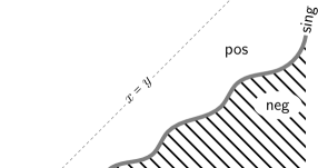
Figure 5. A $\mathsf{pos}$-labelled region delimiting (pseudo-)interval-points.

Lemma 6.

Given a formula $\varphi$ of Cone Logic, if $\mathcal{P}={\langle\mathbb{P},(R_{a})_{a\in\Sigma^{\prime}}\rangle}$ is a labelled rational plane that satisfies $\varphi\wedge\psi_{0}$, then there is a labelled rational plane $\mathcal{P}^{\prime}={\langle\mathbb{P},(R^{\prime}_{a})_{a\in\Sigma^{\prime}}\rangle}$ that still satisfies $\varphi\wedge\psi_{0}$ and such that $R^{\prime}_{\mathsf{sing}}={\{(x,x)\,:\,x\in\mathbb{Q}\}}$.

As a preliminary step, we prove that we can “stretch” the $y$-coordinates of a labelled plane $\mathcal{P}$ with respect to any strictly increasing function $f$, without affecting the satisfaction of any of the subformulas:

For every strictly increasing function $f:\mathbb{Q}\rightarrow\mathbb{Q}$, the labelled plane $\mathcal{P}={\langle\mathbb{P},(R_{a})_{a\in\Sigma^{\prime}}\rangle}$ has the same shading as the labelled rational plane $f(\mathcal{P})={\bigl{\langle}f(\mathbb{P}),\big{(}f(R_{a})\big{)}_{a\in\Sigma^{\prime}}\bigr{\rangle}}$, where $f(R)={\bigl{\{}(x,f(y))\,:\,(x,y)\in R\bigr{\}}}$ for all $R\subseteq\mathbb{P}$.

Proof 7.1 (Proof of the claim).

To start with, we observe that $f(\mathbb{Q})$, equipped with the natural ordering of the rational numbers, is a countable dense linear order with no minimum nor maximum elements. Hence $f(\mathcal{P})$ can be given the status of labelled rational plane.

To conclude the proof, it suffices to observe that for all points $(x,y),(x^{\prime},y^{\prime})\in\mathbb{P}$ and all spatial relations $\,\mathbin{\ooalign{\raisebox{-2.2pt}{\includegraphics{figures/symbols.49}}\crcr\scriptsize$\mspace{-3.0mu}d$}}\,$,

$$(x,y)~{}\,\mathbin{\ooalign{\raisebox{-2.2pt}{\includegraphics{figures/symbols.49}}\crcr\scriptsize$\mspace{-3.0mu}d$}}\,~{}(x^{\prime},y^{\prime})\qquad\text{iff}\qquad(x,f(y))~{}\,\mathbin{\ooalign{\raisebox{-2.2pt}{\includegraphics{figures/symbols.49}}\crcr\scriptsize$\mspace{-3.0mu}d$}}\,~{}(x^{\prime},f(y^{\prime})).$$

Using to the view-to-type dependency, we derive $\mathsf{type}_{\mathcal{P}}(x,y)=\mathsf{type}_{f(\mathcal{P})}(x,f(y))$ for all points $(x,y)\in\mathbb{P}$, which shows that $\mathsf{type}_{\mathcal{P}}(\mathbb{P})=\mathsf{type}_{f(\mathcal{P})}(f(\mathbb{P}))$.

Proof 7.2 (Proof of Lemma 6).

Let $\mathcal{P}={\langle\mathbb{P},(R_{a})_{a\in\Sigma^{\prime}}\rangle}$ be a model for the formula $\varphi\wedge\psi_{0}$. By the definition of $\psi_{0}$, there is a function $f:\mathbb{Q}\rightarrow\mathbb{Q}$ such that for all $x\in\mathbb{Q}$, $(x,y)\in R_{\mathsf{sing}}$ if and only if $y=f(x)$ (this is enforced by the third line of the definition of $\psi_{0}$). By the definition of $\psi_{0}$, it holds that $f$ is strictly increasing: if $x<x^{\prime}$, then $(x,f(x))$ and $(x^{\prime},f(x^{\prime}))$ are two points in $R_{\mathsf{sing}}$ such that $(x,f(x))~{}\,\raisebox{-2.2pt}{\includegraphics{figures/symbols.36}}\,~{}(x^{\prime},f(x^{\prime}))$, and thus $f(x)<f(x^{\prime})$.

Now, let us denote by $f^{-1}$ the inverse of the function $f$, which is also strictly increasing. By the previous claim, we know that the “stretched” labelled plane $\mathcal{P}^{\prime}=f^{-1}(\mathcal{P})$, which is obtained by mapping each point $(x,y)$ of $\mathcal{P}$ to the point $(x,f^{-1}(y))$, has the same shading as $\mathcal{P}$, and hence it also satisfies the formula $\varphi\wedge\psi_{0}$. Moreover, by construction, the region of all $\mathsf{sing}$-labelled points in $\mathcal{P}^{\prime}$ coincides with the diagonal of $\mathcal{P}^{\prime}$:

$$f^{-1}(R_{\mathsf{sing}})~{}=~{}{\bigl{\{}(x,f^{-1}(y))\,:\,(x,y)\in R_{\mathsf{sing}}\bigr{\}}}~{}=~{}{\bigl{\{}(x,f^{-1}(f(x))\,:\,x\in\mathbb{Q}\bigr{\}}}.$$

This shows that the $\mathsf{pos}$-labelled points of $\mathcal{P}^{\prime}$ are exactly the interval-points.

Making use of Lemma 6, we can translate any formula $\varphi$ of the logic $B\bar{B}D\bar{D}L\bar{L}$ into an equi-satisfiable formula $\tilde{\varphi}$ of Cone Logic, which is obtained by first replacing each occurrence of a subformula ${\langle D\rangle}\alpha$ (resp., ${\langle\bar{D}\rangle}\alpha$, ${\langle B\rangle}\alpha$, ${\langle\bar{B}\rangle}\alpha$, ${\langle L\rangle}\alpha$, ${\langle\bar{L}\rangle}\alpha$) in $\varphi$ by the formula $\,\raisebox{-2.7pt}{\includegraphics{figures/symbols.20}}(\mathsf{pos}\wedge\alpha)$ (resp., $\,\raisebox{-2.7pt}{\includegraphics{figures/symbols.19}}(\mathsf{pos}\wedge\alpha)$, $\,\raisebox{-2.7pt}{\includegraphics{figures/symbols.33}}(\mathsf{pos}\wedge\alpha)$, $\,\raisebox{-2.7pt}{\includegraphics{figures/symbols.32}}(\mathsf{pos}\wedge\alpha)$, $\,\mspace{1.7mu}\raisebox{-1.6pt}{\includegraphics{figures/symbols.6}}\mspace{1.7mu}(\mathsf{pos}\rightarrow\,\raisebox{-2.7pt}{\includegraphics{figures/symbols.18}}(\mathsf{pos}\wedge\alpha))$, $\,\mspace{1.7mu}\raisebox{-1.6pt}{\includegraphics{figures/symbols.6}}\mspace{1.7mu}(\mathsf{pos}\rightarrow\,\raisebox{-2.7pt}{\includegraphics{figures/symbols.21}}(\mathsf{pos}\wedge\alpha))$) and then adding the conjunct $\psi_{0}$.

We can easily check the correctness of the translation for modalities ${\langle D\rangle}$, ${\langle\bar{D}\rangle}$, ${\langle B\rangle}$, and ${\langle\bar{B}\rangle}$. Proving that the translation of modalities ${\langle L\rangle}$ and ${\langle\bar{L}\rangle}$ is correct as well is less straightforward. Let us consider an interval $I=[x,y]$ and a later interval $I^{\prime}=[x^{\prime},y^{\prime}]$ of $I$, with $x^{\prime}>y$. Figure 6 depicts the spatial relationships between the corresponding interval-points $p=(x,y)$ and $p^{\prime}=(x^{\prime},y^{\prime})$ and the intermediate point $q=(y,y)$. Clearly, for every interval-point $q^{\prime}$ such that $p\,\,\raisebox{-2.2pt}{\includegraphics{figures/symbols.42}}\,\,q^{\prime}$, we have $q^{\prime}\,\,\raisebox{-2.2pt}{\includegraphics{figures/symbols.40}}\,\,q$ and $q\,\,\raisebox{-2.2pt}{\includegraphics{figures/symbols.36}}\,\,p^{\prime}$, and hence $q^{\prime}\,\,\raisebox{-2.2pt}{\includegraphics{figures/symbols.36}}\,\,p^{\prime}$. Conversely, if $p=(x,y)$ and $p^{\prime}=(x^{\prime},y^{\prime})$ are two interval-points such that $p\,\,\raisebox{-2.2pt}{\includegraphics{figures/symbols.42}}\,\,q^{\prime}$ implies $q^{\prime}\,\,\raisebox{-2.2pt}{\includegraphics{figures/symbols.36}}\,\,p^{\prime}$ for all interval-points $q^{\prime}$, then we necessarily have $x^{\prime}>y$ and hence $I^{\prime}=[x^{\prime},y^{\prime}]$ is a later interval of $I=[x,y]$. This shows that the translation that replaces each occurrence of a subformula ${\langle L\rangle}\alpha$ by the formula $\,\mspace{1.7mu}\raisebox{-1.6pt}{\includegraphics{figures/symbols.6}}\mspace{1.7mu}(\mathsf{pos}\rightarrow\,\raisebox{-2.7pt}{\includegraphics{figures/symbols.18}}(\mathsf{pos}\wedge\alpha))$ is correct. Similar arguments can be used to prove the correctness of the translation for ${\langle\bar{L}\rangle}$.

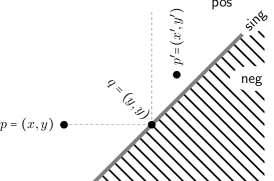
Figure 6. Spatial relationship between an interval-point and its future.

Now, the translation of $B\bar{B}D\bar{D}L\bar{L}$ formulas into equi-satisfiable Cone Logic formulas, together with the decidability result given in Section 6, yields a PSpace procedure to decide the satisfiability problem for the logic $B\bar{B}D\bar{D}L\bar{L}$ when the underlying domain is assumed to be dense. This subsumes previous results from [6]. Moreover, we know from [26] that the satisfiability problem for the interval logic that only uses the subinterval operator ${\langle D\rangle}$ is already PSpace-hard over dense domains. We can thus sum up with the following theorem.

Theorem 7.

The satisfiability problem of Cone Logic over the rational plane and that of the interval temporal logic $B\bar{B}D\bar{D}L\bar{L}$ over $\mathbb{Q}$ are PSpace-complete.

Thanks to the above theorem and Remark 1, we know that the satisfiability problem for Cone Logic interpreted over the class of all labelled planes (including the rational and the real labelled planes) and that of the interval temporal logic $B\bar{B}D\bar{D}L\bar{L}$ interpreted over the class of all dense temporal domains are PSpace-complete. Finally, we point out that similar decidability results hold for the logic $E\bar{E}D\bar{D}L\bar{L}$, by simply changing the orientation of the $x$- and $y$-axes.

8. Conclusions

In this paper, we investigated the satisfiability problem for a suitable weakening of Venema’s Compass Logic, called Cone Logic, and we proved that, unlike the cases of Compass Logic and other projection-based spatial logics, it is decidable (PSpace-complete) over the rational plane $\mathbb{Q}\times\mathbb{Q}$. Moreover, we showed that such a decidability result can be exploited to prove the decidability of the interval temporal logic $B\bar{B}D\bar{D}L\bar{L}$ of Allen’s relations ‘Begins’, ‘During’, and ‘Later’, and their transposes, over the class of dense linear orders (equivalently, the rational numbers), thus disproving a conjecture by Lodaya [12].

One may consider possible extensions of Cone Logic in various directions. For instance, one may consider multi-dimensional spaces and introduce a corresponding logic to describe spatial relationships over points in these spaces (in general, $2^{n}$ distinct cone-shaped directions exist in a space with $n$ dimensions). Alternatively, one may partition the two-dimensional space into more than four cone-shaped directions. In all such cases, we believe it possible to generalize the achieved results, e.g., the tree pseudo-model property, in a rather natural way (the complexity of the satisfiability problem, however, may increase significantly). Other generalizations of Cone Logic envisage the use of region-based relationships. As an example, the correspondence between intervals over the rational line and points over the rational plane can be lifted to higher-dimensional objects, proving, for instance, that a suitable spatial logic based on rectangular regions, that is, two-dimensional intervals, is subsumed by a four-dimensional point-based modal logic very similar to Cone Logic. This would establish a first interesting bridge between Cone Logic and relativistic temporal logics based on Minkowski’s space-time structure [26].

The most interesting open problem is that of determining whether or not Cone Logic remains decidable when interpreted over the real plane $\mathbb{R}\times\mathbb{R}$. In Remark 1, we have seen that, if a Cone Logic formula holds over $\mathbb{R}\times\mathbb{R}$, then it also holds over $\mathbb{Q}\times\mathbb{Q}$. The converse does not hold in general, as there exist formulas of Cone Logic, e.g., that of Example 2, that hold over $\mathbb{Q}\times\mathbb{Q}$, but not over $\mathbb{R}\times\mathbb{R}$. The satisfiability problem for Cone Logic over $\mathbb{R}\times\mathbb{R}$ is not known to be decidable, and the same applies to the interval temporal logic $B\bar{B}D\bar{D}L\bar{L}$ interpreted over $\mathbb{R}$. We plan to study these decidability problems in the future.

Acknowledgments. The authors would like to thank the anonymous reviewers and Dario Della Monica for their valuable comments on a preliminary draft of this paper.

References

- [1] M. Aiello, I. Pratt-Hartmann, and J. van Benthem. Handbook of Spatial Logics. Springer, 2007.
- [2] J.F. Allen. Maintaining knowledge about temporal intervals. Communications of the Association for Computing Machinery, 26(11):832–843, 1983.
- [3] B. Bennett. Modal logics for qualitative spatial reasoning. Bulletin of the Interest Group in Pure and Applied Logic, 4(1):23–45, 1996.
- [4] B. Bennett, A.G. Cohn, F. Wolter, and M. Zakharyaschev. Multi-dimensional modal logic as a framework for spatio-temporal reasoning. Applied Intelligence, 17(3):239–251, 2002.
- [5] D. Bresolin, D. Della Monica, V. Goranko, A. Montanari, and G. Sciavicco. The dark side of interval temporal logic: Sharpening the undecidability border. Annals of Mathematics and Artificial Intelligence, 71(1-3):41–83, 2014.
- [6] D. Bresolin, V. Goranko, A. Montanari, and P. Sala. Tableaux for logics of subinterval structures over dense orderings. Journal of Logic and Computation, 20(1):133–166, 2010.
- [7] E.M. Clarke and E.A. Emerson. Design and synthesis of synchronization skeletons using branching-time temporal logic. In Workshop on Logics of Programs, volume 131 of Lecture Notes in Computer Science, pages 52–71. Springer, 1982.
- [8] M.J. Egenhofer and R. Franzosa. Point-set topological spatial relations. International Journal of Geographic Information Systems, 5(2):161–174, 1991.
- [9] A.U. Frank. Qualitative spatial reasoning about distances and directions in geographic space. Journal of Visual Languages and Computing, 3:343–371, 1992.
- [10] D.M. Gabbay, A. Kurucz, F. Wolter, and M. Zakharyaschev. Many-Dimensional Modal Logics: theory and applications, volume 148 of Studies in Logic and the Foundations of Mathematics. Elsevier Science Publishers, 2003.
- [11] J.Y. Halpern and Y. Shoham. A propositional modal logic of time intervals. Journal of the Association for Computing Machinery, 38:279–292, 1991.
- [12] K. Lodaya. Sharpening the undecidability of interval temporal logic. In Proceedings of the 6th Asian Computing Science Conference on Advances in Computing Science, volume 1961 of Lecture Notes in Computer Science, pages 290–298. Springer, 2000.
- [13] C. Löding and W. Thomas. Alternating automata and logics over infinite words. In Proceedings of the International Conference IFIP on Theoretical Computer Science, Exploring New Frontiers of Theoretical Informatics, volume 1872 of LNCS, pages 521–535. Springer, 2000.
- [14] C. Lutz and F. Wolter. Modal logics of topological relations. Logical Methods in Computer Science, 2(2):1–41, 2006.
- [15] J. Marcinkowski and J. Michaliszyn. The ultimate undecidability result for the Halpern-Shoham logic. In Proc. of the 26th Annual IEEE Symposium on Logic in Computer Science, pages 377–386. IEEE Computer Society, 2011.
- [16] J. Marcinkowski and J. Michaliszyn. The undecidability of the logic of subintervals. Fundamenta Informaticae, 131(2):217–240, 2014.
- [17] M. Marx and M. Reynolds. Undecidability of compass logic. Journal of Logic and Computation, 9(6):897–914, 1999.
- [18] A. Meier, M. Mundhenk, M. Thomas, and H. Vollmer. The complexity of satisfiability for fragments of CTL and CTL*. Electronic Notes in Theoretical Computer Science, 223:201–213, 2008.
- [19] A. Montanari, G. Puppis, and P. Sala. A decidable spatial logic with cone-shaped cardinal directions. In Proceedings of the 18th EACSL Annual Conference on Computer Science Logic, volume 5771 of Lecture Notes in Computer Science, pages 394–408. Springer, 2009.
- [20] A. Morales, I. Navarrete, and G. Sciavicco. A new modal logic for reasoning about space: spatial propositional neighborhood logic. Annals of Mathematics and Artificial Intelligence, 51(1):1–25, 2007.
- [21] A. Morgenstern and K. Schneider. From LTL to symbolically represented deterministic automata. In Proceedings of the 9th International Conference on Verification, Model Checking, and Abstract Interpretation, volume 4905 of LNCS, pages 279–293. Springer, 2008.
- [22] C.M. Papadimitriou. Computational Complexity. Addison-Wesley Longman Publishing Co., Inc., 1994.
- [23] D. Randell, Z. Cui, and A. Cohn. A spatial logic based on regions and connection. In Proceedings of the 3rd International Conference on Principles of Knowledge Representation and Reasoning (KR), pages 165–176, 1992.
- [24] M. Reynolds and M. Zakharyaschev. On the products of linear modal logics. Journal of Logic and Computation, 11(6):909–931, 2001.
- [25] K. Segerberg. Two-dimensional modal logic. Journal of Philosophical Logic, 2(1):77–96, 1973.
- [26] I. Shapirovsky and V.B. Shehtman. Chronological future modality in Minkowski spacetime. In Proceedings of the 4th Conference on Advances in Modal Logic, pages 437–460. King’s College Publications, 2003.
- [27] O. Stock. Spatial and Temporal Reasoning. Kluwer Academic, 1997.
- [28] Y. Venema. Expressiveness and completeness of an interval tense logic. Notre Dame Journal of Formal Logic, 31(4):529–547, 1990.