Penalized estimation in large-scale generalized linear array models

Abstract

Large-scale generalized linear array models (GLAMs) can be challenging to fit. Computation and storage of its tensor product design matrix can be impossible due to time and memory constraints, and previously considered design matrix free algorithms do not scale well with the dimension of the parameter vector. A new design matrix free algorithm is proposed for computing the penalized maximum likelihood estimate for GLAMs, which, in particular, handles nondifferentiable penalty functions. The proposed algorithm is implemented and available via the R package glamlasso. It combines several ideas – previously considered separately – to obtain sparse estimates while at the same time efficiently exploiting the GLAM structure. In this paper the convergence of the algorithm is treated and the performance of its implementation is investigated and compared to that of glmnet on simulated as well as real data. It is shown that the computation time for glamlasso scales favorably with the size of the problem when compared to glmnet. Supplemental materials are available online.

Keywords: penalized estimation, generalized linear array models, proximal gradient algorithm, multidimensional smoothing

1 Introduction

The generalized linear array models (GLAMs) were introduced in Currie et al. (2006) as generalized linear models (GLMs) where the observations can be organized in an array and the design matrix has a tensor product structure. One main application treated in Currie et al. (2006) – that will also be central to this paper – is multivariate smoothing where data is observed on a multidimensional grid.

In this paper we present results on 3-dimensional smoothing for two quite different real data sets where the aim was to extract a smooth mean signal. The first data set contains voltage sensitive dye recordings of spiking neurons in a live ferret brain and was modeled in a Gaussian GLAM framework. The second data set contains all registered Medallion taxi pick ups in New York City during 2013 and was modeled in a Poisson GLAM framework. In both examples we fitted an $\ell_{1}$-penalized B-spline basis expansion to obtain a clear signal. For the taxi data we also demonstrate how the $\ell_{1}$-penalized fit lead to a lower error, compared to the non-penalized fit, when trying to predict missing observations. Other potential applications include factorial designs and contingency tables.

Currie et al. (2006) showed how the structure of GLAMs can be exploited for computing the maximum likelihood estimate and other quantities of importance for statistical inference. The penalized maximum likelihood estimate for a quadratic penalty function can also be computed easily by similar methods. The computations are simple to implement efficiently in any high level language like R or MATLAB that supports fast numerical linear algebra routines. They exploit the GLAM structure to carry out linear algebra operations involving only the tensor factors – called array arithmetic, see also De Boor (1979) and Buis and Dyksen (1996) – and they avoid forming the design matrix. This design matrix free approach offers benefits in terms of memory as well as time usage compared to standard GLM computations.

The approach in Currie et al. (2006) has some limitations when the dimension $p$ of the parameter vector becomes large. The $p\times p$ weighted cross-product of the design matrix has to be computed, and though this computation can benefit from the GLAM structure, a linear equation in the parameter vector remains to be solved. The computations can become prohibitive for large $p$. Moreover, the approach does not readily generalize to non-quadratic penalty functions like the $\ell_{1}$-penalty or for that matter non-convex penalty functions like the smoothly clipped absolute deviation (SCAD) penalty.

In this paper we investigate the computation of the penalized maximum likelihood estimate in GLAMs for a general convex penalty function. However, we note that by employing the multi-step adaptive lasso (MSA-lasso) algorithm from Sections 2.8.5 and 2.8.6 in Bühlmann and van de Geer (2011) our algorithm can easily be extended to handle non-convex penalty functions. This modification is already implemented in the R-package glamlasso for the SCAD-penalty, see Lund (2016). The convergence results presented in this paper are, however, only valid for a convex penalty.

Algorithms considered in the literature hitherto for $\ell_{1}$-penalized estimation in GLMs, see e.g. Friedman et al. (2010), cannot easily benefit from the GLAM structure, and typically they need the design matrix explicitly or at least direct access to its columns. Our proposed algorithm based on proximal operators is design matrix free – in the sense that the tensor product design matrix need not be computed – and can exploit the GLAM structure, which results in an algorithm that is both memory and time efficient.

The paper is organized as follows. In Section 2 GLAMs are introduced. In Section 3 our proposed GD-PG algorithm for computing the penalized maximum likelihood estimate is described. Section 4 presents two multivariate smoothing examples where the algorithm is used to fit GLAMs. This section includes a benchmark comparison between our implementation of the GD-PG algorithm in the R package glamlasso and the algorithm implemented in glmnet. Section 5 presents a convergence analysis of the proposed algorithm. In Section 6 a number of details on how the algorithm is implemented in glamlasso are collected. This includes details on how the GLAM structure is exploited, and the section also presents further benchmark results. Section 7 concludes the paper with a discussion. Some technical and auxiliary definitions and results are presented in two appendices.

2 Generalized linear array models

A generalized linear model (GLM) is a regression model of $n$ independent real valued random variables $\mathcal{Y}_{1},\ldots,\mathcal{Y}_{n}$, see Nelder and Wedderburn (1972). A generalized linear array model (GLAM) is a GLM with some additional structure of the data. We first introduce GLMs and then the special data structure for GLAMs.

With $X$ an $n\times p$ design matrix, the linear predictor $\eta:\mathbb{R}^{p}\to\mathbb{R}^{n}$ is defined as

$$\eta(\theta)\coloneqq X\theta$$ (1)

for $\theta\in\mathbb{R}^{p}$. With $g:\mathbb{R}\to\mathbb{R}$ denoting the link function, the mean value of $\mathcal{Y}_{i}$ is given in terms of $\eta_{i}(\theta)$ via the equation

$$g(\operatorname{E}(\mathcal{Y}_{i}))=\eta_{i}(\theta).$$ (2)

The link function $g$ is throughout assumed invertible with a continuously differentiable inverse.

The distribution of $\mathcal{Y}_{i}$ is, furthermore, assumed to belong to an exponential family, see Appendix B, which implies that the log-likelihood, $\theta\mapsto l(\eta(\theta))$, is given in terms of the linear predictor. With $y=(y_{1},\ldots,y_{n})^{\top}\in\mathbb{R}^{n}$ denoting a vector of realized observations of the variables $\mathcal{Y}_{i}$, the log-likelihood (with weights $a_{i}\geq 0$ for $i=1,\ldots,n$) and its gradient are given as

$$l(\eta(\theta)) =\sum_{i=1}^{n}a_{i}(y_{i}\vartheta(\eta_{i}(\theta))-b(\vartheta(\eta_{i}(\theta))))\quad\textnormal{and}$$ (3)

$$\nabla_{\theta}l(\eta(\theta)) =X^{\top}u(\eta(\theta)),$$ (4)

respectively, where $\vartheta:\mathbb{R}\to\mathbb{R}$ denotes the canonical parameter function, and $u(\eta)\coloneqq\nabla_{\eta}l(\eta)$ is the score statistic, see Appendix B.

The main problem considered in this paper is the computation of the penalized maximum likelihood estimate (PMLE),

$$\theta^{\ast}\coloneqq\operatorname*{arg\,min}_{\theta\in\mathbb{R}^{p}}-l(\eta(\theta))+\lambda J(\theta),$$ (5)

where $J:\mathbb{R}^{p}\to(-\infty,\infty]$ is a proper, convex and closed penalty function, and $\lambda\geq 0$ is a regularization parameter controlling the amount of penalization. Note that $J$ is allowed to take the value $\infty$, which can be used to enforce convex parameter constraints. The objective function of this minimization problem is thus the penalized negative log-likelihood, denoted

$$F\coloneqq-l+\lambda J,$$ (6)

where $-l$ is continuously differentiable.

For a GLAM the vector $y$ is assumed given as $y=\operatorname{vec}(Y)$ (the $\operatorname{vec}$ operator is discussed in Appendix A), where $Y$ is an $n_{1}\times\cdots\times n_{d}$ $d$-dimensional array. The design matrix $X$ is assumed to be a concatenation of $c$ matrices

$$X=[X_{1}|X_{2}|\ldots|X_{c}],$$

where the $r$th component is a tensor product,

$$X_{r}=X_{r,d}\otimes X_{r,d-1}\otimes\cdots\otimes X_{r,1},$$ (7)

of $d$ matrices. The matrix $X_{r,j}$ is an $n_{j}\times p_{r,j}$ matrix, such that

$$n=\prod_{j=1}^{d}n_{j},\quad p_{r}\coloneqq\prod_{j=1}^{d}p_{r,j},\quad p=\sum_{r=1}^{c}p_{r}.$$

We let $\langle X_{r,j}\rangle\coloneqq\langle X_{1,1},\ldots,X_{c,d}\rangle$ denote the tuple of marginal design matrices.

The assumed data structure induces a corresponding structure on the parameter vector, $\theta$, as a concatenation of $c$ vectors,

$$\theta^{\top}=(\operatorname{vec}(\Theta_{1})^{\top},\ldots,\operatorname{vec}(\Theta_{c})^{\top}),$$

with $\Theta_{r}$ a $p_{r,1}\times\cdots\times p_{r,d}$ $d$-dimensional array. We let $\langle\Theta_{r}\rangle\coloneqq\langle\Theta_{1},\ldots,\Theta_{c}\rangle$ denote the tuple of parameter arrays.

Given this structure it is possible to define a map, $\rho$, such that with $\theta_{r}=\operatorname{vec}(\Theta_{r})$,

$$X_{r}\theta_{r}=\operatorname{vec}\big{(}\rho(X_{r,d},\ldots,\rho(X_{r,2},(\rho(X_{r,1},\Theta_{r})))\ldots)\big{)}$$ (8)

for $r=1,\ldots,c$. The algebraic details of $\rho$ are spelled out in Appendix A.

As a consequence of the array structure, the linear predictor can be computed using $\rho$ without explicitly constructing $X$. The most obvious benefit is that no large tensor product matrix needs to be computed and stored. In addition, the array structure can be beneficial in terms of time complexity. As noted in Buis and Dyksen (1996), with $X_{r,j}$ being a square $n_{r}\times n_{r}$ matrix, say, the computation of the direct matrix-vector product in (8) has $O(n_{r}^{2d})$ time complexity, while the corresponding array computation has $O(dn_{r}^{d+1})$ time complexity. This reduced time complexity for $d\geq 2$ translates, as mentioned in the introduction, directly into a computational advantage for computing the PMLE with a quadratic penalty function, see Currie et al. (2006). For non-quadratic penalty functions the translation is less obvious, but we present one algorithm that is capable of benefitting from the array structure.

3 Penalized estimation in a GLAM

In most situations the PMLE must be computed by an iterative algorithm. We present an algorithm that solves the optimization problem (5) by iteratively optimizing a partial quadratic approximation to the objective function while exploiting the array structure. The proposed algorithm is a combination of a gradient based descent (GD) algorithm with a proximal gradient (PG) algorithm. The resulting algorithm, which we call GD-PG, thus consists of the following two parts:

• an outer GLAM enhanced GD loop

• an inner GLAM enhanced PG loop.

We present these two loops in the sections below postponing the details on how the array structure can be exploited to Section 6, where it is explained in detail how the two loops can be enhanced for GLAMs.

3.1 The outer GD loop

The outer loop consists of a sequence of descent steps based on a partial quadratic approximation of the objective function. This results in a sequence of estimates, each of which is defined in terms of a penalized weighted least squares estimate and whose computation involves an iterative choice of weights. The weights can be chosen so that the inner loop can better exploit the array structure.

For $k\in\mathbb{N}$ and $\theta^{(k)}\in\mathbb{R}^{p}$ let $\eta^{(k)}=\eta(\theta^{(k)})$ and $u^{(k)}=\nabla_{\eta}l(\eta^{(k)})$, let $W^{(k)}$ denote a positive definite diagonal $n\times n$ weight matrix and let $z^{(k)}$ denote the $n$-dimensional vector (the working response) given by

$$z^{(k)}\coloneqq(W^{(k)})^{-1}u^{(k)}+\eta^{(k)}.$$ (9)

The sequence $(\theta^{(k)})$ is defined recursively from an initial $\theta^{(0)}$ as follows. Given $\theta^{(k)}$ let

$$\tilde{\theta}^{(k+1)}\coloneqq\operatorname*{arg\,min}_{\theta\in\mathbb{R}^{p}}\frac{1}{2n}\|\sqrt{W^{(k)}}(X\theta-z^{(k)})\|^{2}_{2}+\lambda J(\theta)$$ (10)

denote the penalized weighted least squares estimate and define

$$\theta^{(k+1)}\coloneqq\theta^{(k)}+\alpha_{k}(\tilde{\theta}^{(k+1)}-\theta^{(k)}),$$ (11)

where the stepsize $\alpha_{k}>0$ is determined to ensure sufficient descent of the objective function, e.g. by using the Armijo rule. A detailed convergence analysis is given in Section 5, where the relation to the class of gradient based descent algorithms in Tseng and Yun (2009) is established.

3.2 The inner PG loop

The inner loop solves (10) by a proximal gradient algorithm. To formulate the algorithm consider a generic version of (10) given by

$$x^{\ast}\coloneqq\operatorname*{arg\,min}_{x\in\mathbb{R}^{p}}h(x)+\lambda J(x),$$ (12)

where $h:\mathbb{R}^{p}\to\mathbb{R}$ is convex and continuously differentiable. It is assumed that there exists a minimizer $x^{\ast}$. Define for $\gamma>0$ the proximal operator, $\mathrm{prox}_{\gamma}:\mathbb{R}^{p}\to\mathbb{R}^{p}$, by

$$\mathrm{prox}_{\gamma}(z)=\operatorname*{arg\,min}_{x\in\mathbb{R}^{p}}\Big{\{}\frac{1}{2}\|x-z\|_{2}^{2}+\gamma J(x)\Big{\}}.$$

The proximal operator is particularly easy to compute for a separable penalty function like the 1-norm or the squared 2-norm. Given a stepsize $\delta_{k}>0$, initial values $x^{(0)}=x^{(1)}\in\mathbb{R}^{p}$ and an extrapolation sequence $(\omega_{l})$ with $\omega_{l}\in[0,1)$ define the sequence $(x^{(l)})$ recursively by

$$y \coloneqq x^{(l)}+\omega_{l}\Big{(}x^{(l)}-x^{(l-1)}\Big{)}\quad\textrm{and}$$ (13)

$$x^{(l+1)} \coloneqq\mathrm{prox}_{\delta_{k}\lambda}(y-\delta_{k}\nabla h(y)).$$ (14)

The choice of $\omega_{l}=0$ for all $l\in\mathbb{N}$ gives the classical proximal gradient algorithm, see Parikh and Boyd (2014). Other choices of the extrapolation sequence, e.g. $\omega_{l}=(l-1)/(l+2)$, can accelerate the convergence. Convergence results can be established if $\nabla h$ is Lipschitz continuous and $\delta_{k}$ is chosen sufficiently small – see Section 5 for further details.

For the convex function

$$h(\theta) \coloneqq\frac{1}{2n}\|\sqrt{W^{(k)}}(X\theta-z^{(k)})\|^{2}_{2}$$ (15)

we have that

$$\nabla h(\theta)=\frac{1}{n}X^{\top}W^{(k)}(X\theta-z^{(k)}).$$ (16)

This shows that $\nabla h(\theta)$ is Lipschitz continuous, and its explicit form in (16) indicates how the array structure can be exploited – see also Section 6.

3.3 The GD-PG algorithm

The combined GD-PG algorithm is outlined as Algorithm 1 below. It is formulated using array versions of the model components. Especially, $U^{(k)}$ and $Z^{(k)}$ denote $n_{1}\times\cdots\times n_{d}$ array versions of the score statistic, $u^{(k)}$, and the working response, $z^{(k)}$, respectively. Also $V^{(k)}$ is an $n_{1}\times\cdots\times n_{d}$ array containing the diagonal of the $n\times n$ weight matrix $W^{(k)}$. The details on how the steps in the algorithm can exploit the array structure are given in Section 6.

Algorithm 1 GD-PG

0:  $\langle\Theta_{r}^{(0)}\rangle$, $\langle X_{r,j}\rangle$

1:  for $k=0$ to $K\in\mathbb{N}$ do

2:     given $\langle\Theta_{r}^{(k)}\rangle$: compute $U^{(k)}$, specify $V^{(k)}$ and compute $Z^{(k)}$

3:     specify the proximal stepsize $\delta_{k}$

4:     given $\langle\Theta_{r}^{(k)}\rangle,V^{(k)},Z^{(k)},\delta_{k}$: compute $\langle\tilde{\Theta}_{r}^{(k+1)}\rangle$ by the inner PG loop

5:     given $\langle\Theta_{r}^{(k)}\rangle,\langle\tilde{\Theta}_{r}^{(k+1)}\rangle$: use a line search to compute $\langle\Theta_{r}^{(k+1)}\rangle$

6:     if convergence criterion is satisfied then

7:        break

8:     end if

9:  end for

The outline of Algorithm 1 leaves out some details that are required for an implementation. In step 2 the weights must be specified. In Section 5 we present results on convergence of the outer loop, which put some restrictions on the choice of weights. In step 3 the proximal gradient stepsize must be specified. In Section 5 we give a computable upper bound on the stepsize that ensures convergence of the inner PG loop. Convergence with the same convergence rate can also be ensured for larger stepsizes if a backtracking step is added to the inner PG loop. In step 4, $\langle\Theta_{r}^{(k)}\rangle$ is a natural choice of initial value in the inner PG loop, but this choice is not necessary to ensure convergence. In step 4 it is, in addition, necessary to specify the extrapolation sequence. Finally, in step 5 a line search is required. In Section 5 convergence of the outer loop is treated when the Armijo rule is used.

4 Applications to multidimensional smoothing

As a main application of the GD-PG algorithm we consider multidimensional smoothing, which can be formulated in the framework of GLAMs by using a basis expansion with tensor product basis functions. We present the framework below and report the results obtained for two real data sets.

4.1 A generalized linear array model for smoothing

Letting ${\mathcal{X}}_{1},\ldots,{\mathcal{X}}_{d}\subseteq\mathbb{R}$ denote $d$ finite sets define the $d$-dimensional grid

$$\mathcal{G}_{d}\coloneqq{\mathcal{X}}_{1}\times\cdots\times{\mathcal{X}}_{d}.$$

The set ${\mathcal{X}}_{j}$ is the set of (marginal) grid points in the $j$th dimension and $n_{j}\coloneqq|{\mathcal{X}}_{j}|$ denotes the number of such marginal points in the $j$th dimension. We have a total of $n\coloneqq\prod_{j=1}^{d}n_{j}$ $d$-dimensional joint grid points, or $d$-tuples,

$$(x_{1},\ldots,x_{d})\in\mathcal{G}_{d}.$$

For each of the $n$ grid points we observe a corresponding grid value $y_{x_{1},\ldots,x_{d}}\in\mathbb{R}$ assumed to be a realization of a real valued random variable $\mathcal{Y}_{x_{1},\ldots,x_{d}}$ with finite mean. That is, the observations can be regarded as a $d$-dimensional array $Y$. With $g:\mathbb{R}\to\mathbb{R}$ a link function let

$$f(x_{1},\ldots,x_{d})\coloneqq g(\operatorname{E}(\mathcal{Y}_{x_{1},\ldots,x_{d}})),\quad(x_{1},\ldots,x_{d})\in{\mathcal{G}}_{d}.$$ (17)

The objective is to estimate $f$, which is assumed to possess some form of regularity as a function of $(x_{1},\ldots,x_{d})$. Assuming that $f$ belongs to the span of $p$ basis functions, $\phi_{1},\ldots,\phi_{p}$, it holds that

$$f(x_{1},\ldots,x_{d})=\sum_{m=1}^{p}\beta_{m}\phi_{m}(x_{1},\ldots,x_{d}),\quad(x_{1},\ldots,x_{d})\in{\mathcal{G}}_{d},$$

for $\beta\in\mathbb{R}^{p}$. If the basis function evaluations are collected into an $n\times p$ matrix $\Phi\coloneqq(\phi_{m}((x_{1},\ldots,x_{d})_{i}))_{i,m}$, and if the entries in the array $Y$ are realizations of independent random variables from an exponential family as described in Appendix B, the resulting model is a GLM with design matrix $\Phi$ and regression coefficients $\beta$.

For $d\geq 2$ the $d$-variate basis functions can be specified via a tensor product construction in terms of $d$ (marginal) sets of univariate functions by

$$\phi_{m_{1},\ldots,m_{d}}\coloneqq\phi_{1,m_{1}}\otimes\phi_{2,m_{2}}\otimes\cdots\otimes\phi_{d,m_{d}},$$ (18)

where $\phi_{j,m}:\mathbb{R}\to\mathbb{R}$ for $j=1,\ldots,d$ and $m=1,\ldots,p_{j}$. The evaluation of each of the $p_{j}$ univariate functions in the $n_{j}$ points in ${\mathcal{X}}_{j}$ results in an $n_{j}\times p_{j}$ matrix $\Phi_{j}=(\phi_{j,m}(x_{k}))_{k,m}$. It then follows that the $n\times p$ ($p\coloneqq\prod_{j=1}^{d}p_{j}$) tensor product matrix

$$\Phi=\Phi_{d}\otimes\cdots\otimes\Phi_{1}$$ (19)

is identical to the design matrix for the basis evaluation in the tensor product basis, and the GLM has the structure required of a GLAM.

4.2 Benchmarking on real data

The multidimensional smoothing model described in the previous section was fitted using an $\ell_{1}$-penalized B-spline basis expansion to two real data sets using the GD-PG algorithm as implemented in the R package glamlasso. See Section 6.4 for details about the R package. In this section we report benchmark results for glamlasso and the coordinate descent based implementation in the R package glmnet, see Friedman et al. (2010).

For both data sets we fitted a sequence of models to data from an increasing subset of grid points, which correspond to a sequence of design matrices of increasing size. For each design matrix we fitted 100 models for a decreasing sequence of values of the penalty parameter $\lambda$. We report the run time for fitting the sequence of 100 models using glamlasso and glmnet. We also report the run time for the combined computation of the tensor product design matrix and the fit using glmnet. The latter is more relevant for a direct comparison with glamlasso, since glamlasso requires only the marginal design matrices while glmnet requires the full tensor product design matrix.

To justify the comparison we report the relative deviation of the objective function values attained by glamlasso from the objective function values attained by glmnet, that is,

$$\frac{F(\hat{\theta}^{\texttt{glamlasso}})-F(\hat{\theta}^{\texttt{glmnet}})}{|F(\hat{\theta}^{\texttt{glmnet}})|}$$ (20)

with $\hat{\theta}^{\texttt{x}}$ denoting the estimate computed by method x. This ratio is computed for each fitted model. We note that (20) has a tendency to blow up in absolute value when $F$ becomes small, which happens for small values of $\lambda$.

The benchmark computations were carried out on a Macbook Pro with a 2.8 GHz Intel core i7 processor and 16 GB of 1600 MHz DDR3 memory. Scripts and data are included as supplemental materials online.

4.2.1 Gaussian neuron data

The first data set considered consists of spatio-temporal voltage sensitive dye recordings of a ferret brain provided by Professor Per Ebbe Roland, see Roland et al. (2006). The data set consists of images of size $25\times 25$ pixels recorded with a time resolution of 0.6136 ms per image. The images were recorded over 600 ms, hence the total size of this 3-dimensional array data set is $25\times 25\times 977$ corresponding to $n=610,625$ data points.

As basis functions we used cubic B-splines with $p_{j}\coloneqq\max\{[n_{j}/5],5\}$ basis functions in each dimension (see Currie et al. (2006) or Wood (2006)). This corresponds to a parameter array of size $5\times 5\times 196$ ($p=4,900$) and a design matrix of size $610,625\times 4,900$ for the entire data set. The byte size for representing this design matrix as a dense matrix was approximately 22 GB. For the benchmark we fitted Gaussian models with the identity link function to the full data set as well as to subsets of the data set that correspond to smaller design matrices.

Figure 1 shows an example of the raw data and the smoothed fit for a particular time point. Movies of the raw data and the smoothed fit can be found as supplementary material.

Run times and relative deviations are shown in Figure 2. The model could not be fitted using glmnet to the full data set due to the large size of the design matrix, and results for glmnet are thus only reported for models that could be fitted. The run times for glamlasso were generally smaller than for glmnet, and were, in particular, relatively insensitive to the size of the design matrix. When a sparse matrix representation of the design matrix was used, glmnet was able to scale to larger design matrices, but it was still clearly outperformed by glamlasso in terms of run time. The relative deviations in the attained objective function values were quite small.

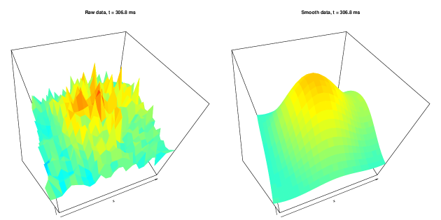
Figure 1: The raw neuron data (left) and the smoothed fit (right) after 306.8 ms. The supplementary material contains movies of the complete raw data and smoothed fit.

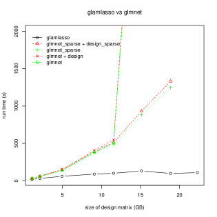
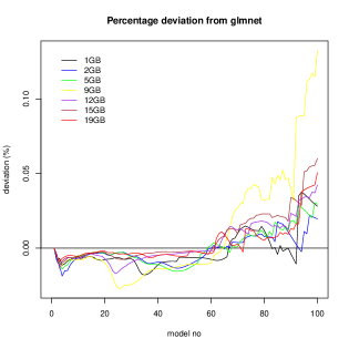
Figure 2: Benchmark results for the neuron data. Run time in seconds is shown as a function of the size of the design matrix, when not stored in sparse format, in GB (left). Relative deviation in the attained objective function values as given by (20) is shown as a function of model number (right), where a larger model number corresponds to less penalization (smaller $\lambda$).

Figure 3: Binned counts of registered NYC taxi pickups for January 2013 using $500\times 500$ spatial bins (left) and the same data rotated, binned to $100\times 100$ spatial bins and cropped to cover Manhattan only (right).

4.2.2 Poisson taxi data

The second data set considered consists of spatio-temporal information on registered taxi pickups in New York City during January 2013. The data can be download from the webpage www.andresmh.com/nyctaxitrips/. We used a subset of this data set consisting of triples containing longitude, latitude and date-time of the pickup. First we cropped the data to pickups with longitude in $[-74.05^{\circ},-73.93^{\circ}]$ and latitude in $[40.7^{\circ},40.82^{\circ}]$. Figure 3 shows the binned counts of all pickups during January 2013 with 500 bins in each spatial dimension. Pickups registered in Hudson or East River were ascribed to noise in the GPS recordings.

For this example attention was restricted to Manhattan pickups during the first week of January 2013. To this end the data was rotated and summarized as binned counts in $100\times 100\times 168$ spatial-temporal bins. Each temporal bin represents one hour. The data was then further cropped to cover Manhattan only, which removed the large black parts – as seen on Figure 3 – where pickups were rare. The total size of the data set was $33\times 81\times 168$ corresponding to $n=449,064$ data points. The observation in each bin consisted of the integer number of pickups registered in that bin.

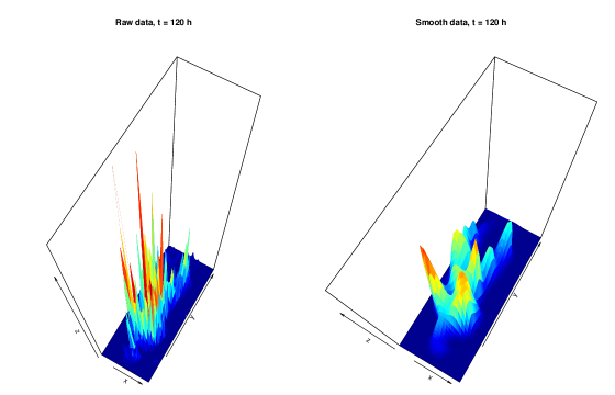
Figure 4: The raw NYC taxi data (left) and the smoothed fit (right) around midnight on Saturday, January 5, 2013. The supplementary material contains movies of the complete raw data and smoothed fit.

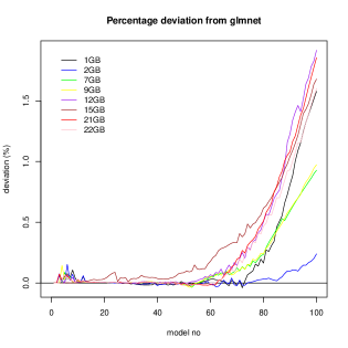
Figure 5: Benchmark results for the taxi data. Run time in seconds is shown as a function of the size of the design matrix, when not stored in sparse format, in GB (left). Relative deviations in the attained objective function values as given by (20) is shown as a function of model number (right), where a larger model number corresponds to less penalization (smaller $\lambda$).

We used $p_{j}\coloneqq\max\{[n_{j}/4],5\}$ cubic B-spline basis functions in each dimension. The resulting parameter array was $9\times 21\times 42$ corresponding to $p=7,938$ and a design matrix of size $449,064\times 7,938$ for the entire data set. The byte size for representing this design matrix as a dense matrix was approximately 27 GB. For the benchmark we fitted Poisson models with the log link function to the full data set as well as to subsets of the data set that correspond to smaller design matrices.

Figure 4 shows an example of the raw data and the smoothed fit for around midnight on Saturday, January 5, 2013. Movies of the raw data and the smoothed fit can be found as supplementary material.

Run times and relative deviations are shown in Figure 5. As for the neuron data, the model could not be fitted to the full data set using glmnet, and results for glmnet are only reported for models that could be fitted. Except for the smallest design matrix the run times for glamlasso were smaller than for glmnet, and they appear to scale better with the size of the design matrix. This was particularly so when the dense matrix representation was used with glmnet. The design matrix was very sparse in this example, and glmnet benefitted considerable in terms of run time from using a sparse storage format. The relative deviations in the attained objective function values were still acceptably small though the values attained by glamlasso were up to 1.5% larger than those attained by glmnet for the least penalized models (models fitted with small values of $\lambda$).

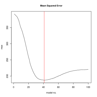
Figure 6: The mean squared error for prediction on grid points left out of the model fitting as a function of model number. The vertical red line indicates the model with minimal MSE (model 41).

4.3 Using incomplete array data

The implementation in glamlasso allows for incompletely observed arrays. This can, of course, be used for prediction of the unobserved entries by computing the smoothed fit to the incompletely observed array. In this section we show how it can also be used for selection of the tuning parameter $\lambda$. We also refer to the supplemental materials online for scripts and data.

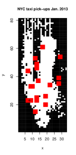
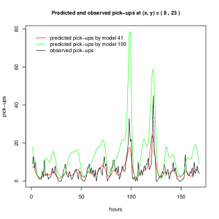
Figure 7: Binned number of NYC taxi pickups as in Figure 3 (left) with red $3\times 3$ squares indicating bins that were removed from the data before model fitting. Predicted and observed number of pickups at spatial bin $(8,23)$ (indicated with a “+” on the left figure) are shown as a function of time in hours (right). Model 100 predictions (green) were from the least penalized model while Model 41 predictions (red) were from the model with an overall minimal MSE.

We used the NYC taxi data and removed the observations for 19 randomly chosen $3\times 3$ blocks of spatial bins (due to overlap of some of the blocks this corresponded to 159 spatial bins). When fitting the model using glamlasso the incompleteness is incorporated by setting the weights corresponding to the missing values equal to zero for all time points. We denote by $D$ the set of grid points that correspond to the removed bins as illustrated by the red blocks in Figure 7.

From glamlasso we computed a sequence of model fits corresponding to 100 values of $\lambda$, and for each value of $\lambda$ we computed the fitted complete array $\hat{Y}^{(\lambda)}$ and then the mean squared error (MSE),

$$\text{MSE}(\lambda)=\sum_{x\in D}(\hat{Y}^{(\lambda)}_{x}-Y_{x})^{2},$$

as a function of $\lambda$, see Figure 6. Model 41 attained the overall minimal MSE.

Figure 7 shows predictions for one spatial bin. The under-smoothed Model 100 gives a poor prediction while the overall optimal Model 41 gives a much better prediction.

5 Convergence analysis

Our proposed GD-PG algorithm is composed of well known components, whose convergence properties have been extensively studied. We do, however, want to clarify under which conditions the algorithm can be shown to converge and in what sense it converges. The main result in this section is a computable upper bound of the step-size, $\delta_{k}$, in the inner PG loop that ensures convergence in this loop. This result hinges on the tensor product structure of the design matrix.

We first state a theorem, which follows directly from Beck and Teboulle (2010), and which for a specific choice of extrapolation sequence gives the convergence rate for the inner PG loop for minimizing the objective function

$$G\coloneqq h+\lambda J,$$ (21)

where $h$ is given by (15). In the following, $\|A\|_{2}$ denotes the spectral norm of $A$, which is the largest singular value of $A$.

Theorem 1.

Let $x^{\ast}=\tilde{\theta}^{(k+1)}$ denote the minimizer defined by (10) and let the extrapolation sequence for the inner PG loop be given by $\omega_{l}=(l-1)/(l+2)$. Let $(x^{(l)})$ denote the sequence obtained from the inner PG loop. If $\delta^{(k)}\in(0,1/L^{(k)}]$ where

$$L^{(k)}:=\|X^{\top}W^{(k)}X\|_{2}/n$$ (22)

then

$$G(x^{(l)})-G(x^{\ast})\leq\frac{2L_{h}^{(k)}\|x^{(0)}-x^{*}\|_{2}^{2}}{(l+1)^{2}}.$$ (23)

Proof.

The theorem is a consequence of Theorem 1.4 in Beck and Teboulle (2010) once we establish that $L^{(k)}$ is a Lipschitz constant for $\nabla h$. To this end note that the spectral norm $\|\cdot\|_{2}$ is the operator norm induced by the 2-norm on $\mathbb{R}^{p}$, which implies that

$$\|\nabla h(\theta)-\nabla h(\theta^{\prime})\|_{2} \leq\frac{1}{n}\|X^{\top}W^{(k)}X\|_{2}\|\theta-\theta^{\prime}\|_{2},$$ (24)

and $L^{(k)}$ is indeed the minimal Lipschitz constant. It should be noted that Theorem 1.4 in Beck and Teboulle (2010) is phrased in terms of an acceleration sequence of the form $\omega_{l}=(t_{l}-1)/t_{l+1}$ where $(t_{l})$ is a specific sequence that fulfills $t_{l}\geq(l+1)/2$. The acceleration sequence considered here corresponds to $t_{l}=(l+1)/2$, and their proof carries over to this case without changes. ∎

From (23) we see that the objective function values converge at rate $O(l^{-2})$ for the given choice of extrapolation sequence. Without extrapolation, that is, with $\omega_{l}=0$ for all $l\in\mathbb{N}$, the convergence rate is $O(l^{-1})$, see e.g. Theorem 1.1 in Beck and Teboulle (2010). In this case $(x^{(l)})$ always converges towards a minimizer, see Theorem 1.2 in Beck and Teboulle (2010). We are not aware of results that establish convergence of $(x^{(l)})$ for general $h$ when extrapolation is used. However, if $X$ has rank $p$ and the weights are all strictly positive, the quadratic $h$ given by (15) results in a strictly convex and level bounded objective function $G$, in which case (23) forces $(x^{(l)})$ to converge towards the unique minimizer.

The following result shows how the tensor product structure can be exploited to give a computable upper bound on the Lipschitz constant (22).

Proposition 1.

Let $W^{(k)}$ denote the diagonal weight matrix with diagonal elements $w_{i}^{(k)}$, $i=1,\ldots,n$, then

$$L^{(k)}\leq\hat{L}^{(k)}\coloneqq\frac{\max(w_{i}^{(k)})}{n}\sum_{r=1}^{c}\prod_{j=1}^{d}\varrho(X_{r,j}^{\top}X_{r,j})$$ (25)

where $\varrho$ denotes the spectral radius.

Proof.

Since the spectral norm is an operator norm it is submultiplicative, which gives that

$$L^{(k)} \leq\frac{1}{n}\|X^{\top}\|_{2}\|X\|_{2}\|W^{(k)}\|_{2}=\frac{1}{n}\|X\|_{2}^{2}\|W^{(k)}\|_{2}.$$ (26)

Now $W^{(k)}$ is diagonal with nonnegative entries, so $\|W^{(k)}\|_{2}=\max(w_{i}^{(k)})$, and $\|X\|_{2}^{2}$ is the largest eigenvalue of the symmetric matrix $X^{\top}X$ (the spectral radius), hence

$$L^{(k)}\leq\frac{\max(w_{i}^{(k)})}{n}\varrho(X^{\top}X).$$ (27)

Furthermore, as $X^{\top}X$ is a positive semidefinite matrix with diagonal blocks given by $X_{r}^{\top}X_{r}$ we get (see e.g. Lemma 3.20 in Bapat (2010)) that

$$\varrho(X^{\top}X)\leq\sum_{r=1}^{c}\varrho(X_{r}^{\top}X_{r}).$$ (28)

By the properties of the tensor product we find that

$$X_{r}^{\top}X_{r}=X_{r,1}^{\top}X_{r,1}\otimes\ldots\otimes X_{r,d}^{\top}X_{r,d},$$ (29)

whose eigenvalues are of the form $\alpha_{1,k_{1}}\alpha_{2,k_{2}}\cdots\alpha_{d,k_{d}}$, with $\alpha_{j,k_{j}}$ being the $k_{j}$th eigenvalue of $X_{r,j}^{\top}X_{r,j}$, see e.g. Theorem 4.2.12 in Horn and Johnson (1991). In particular,

$$\varrho(X_{r}^{\top}X_{r})=\prod_{j=1}^{d}\varrho(X_{r,j}^{\top}X_{r,j}),$$

and this completes the proof. ∎

Note that for $c=1$ the upper bound is $\hat{L}^{(k)}=\max(w_{i}^{(k)})\prod_{j=1}^{d}\varrho(X_{1,j}^{\top}X_{1,j})/n$, which is valid for any weight matrix. If the weight matrix is itself a tensor product it is possible to compute the Lipschitz constant exactly. Indeed, if $W^{(k)}=W^{(k)}_{d}\otimes\ldots\otimes W^{(k)}_{1}$ then

$$X^{\top}W^{(k)}X=X_{1,d}^{\top}W^{(k)}_{d}X_{1,d}\otimes\ldots\otimes X_{1,1}^{\top}W^{(k)}_{1}X_{1,1},$$

and by similar arguments as in the proof above,

$$L^{(k)}=\frac{1}{n}\prod_{j=1}^{d}\varrho(X_{1,j}^{\top}W^{(k)}_{j}X_{1,j}).$$ (30)

The outer loop is similar to the outer loop used in e.g. the R packages glmnet, Friedman et al. (2010), and sglOptim, Vincent et al. (2014). For completeness we demonstrate that the outer loop with the stepsize determined by the Armijo rule is a special case of the algorithm treated in Tseng and Yun (2009), which implies a global convergence result of the outer loop.

Following Tseng and Yun (2009) the Armijo rule gives the stepsize $\alpha_{k}\coloneqq b^{j}\alpha_{0}$, where $\alpha_{0}>0$ and $b\in(0,1)$ are given constants and $j$ is determined as follows: With $d^{(k)}=\tilde{\theta}^{(k+1)}-\theta^{(k)}$ and

$$\Delta_{k}\coloneqq-(u^{(k)})^{\top}Xd^{(k)}+\lambda(J(\tilde{\theta}^{(k+1)})-J(\theta^{(k)})),$$

then $j\in\mathbb{N}_{0}$ is the smallest nonnegative integer for which

$$F(\theta^{(k)}+b^{j}\alpha_{0}d^{(k)})\leq F(\theta^{(k)})+b^{j}\alpha_{0}v\Delta_{k},$$ (31)

where $v\in(0,1)$ is a fixed constant.

Theorem 2.

Let the stepsize, $\alpha_{k}$, be given by the Armijo rule above. If the design matrix $X$ has rank $p$ and if there exist constants $\bar{c}\geq\underline{c}>0$ such that for all $k\in\mathbb{N}$ the diagonal weights in $W^{(k)}$, denoted $w_{i}^{(k)}$, satisfy

$$\underline{c}\leq w_{i}^{(k)}\leq\bar{c}$$ (32)

for $i=1,\ldots,n$, then $(F(\theta^{(k)}))$ is nonincreasing and any cluster point of $(\theta^{(k)})$ is a stationary point of the objective function $F$.

Proof.

The theorem is a consequence of Theorem 1 (a) and (e) in Tseng and Yun (2009) once we have established that the search direction, $d^{(k)}=\tilde{\theta}^{(k+1)}-\theta^{(k)}$, coincides with the search direction defined by (6) in Tseng and Yun (2009). Letting $d\coloneqq\theta-\theta^{(k)}$ denote a (potential) search direction we see that

$$\frac{1}{2n}\| \sqrt{W^{(k)}}(X\theta-z^{(k)})\|^{2}_{2}$$

$$=\frac{1}{2n}(-(W^{(k)})^{-1}u^{(k)}+X(\theta-\theta^{(k)}))^{\top}W^{(k)}(-(W^{(k)})^{-1}u^{(k)}+X(\theta-\theta^{(k)}))$$

$$=\frac{1}{2n}((u^{(k)})^{\top}(W^{(k)})^{-1}u^{(k)}-(u^{(k)})^{\top}Xd-d^{\top}X^{\top}u^{(k)}+d^{\top}X^{\top}W^{(k)}Xd)$$

$$\propto-\underbrace{(u^{(k)})^{\top}X}_{\nabla_{\theta}l(\eta^{(k)})^{\top}}d+\frac{1}{2}d^{\top}\underbrace{X^{\top}W^{(k)}X}_{H^{(k)}}d+C_{k},$$

where $C_{k}$ is a constant not depending upon $\theta$. This shows that

$$d^{(k)}=\operatorname*{arg\,min}_{d\in\mathbb{R}^{p}}-\nabla_{\theta}l(\eta^{(k)})^{\top}d+\frac{1}{2}d^{\top}H^{(k)}d+\lambda J(\theta^{(k)}+d),$$ (33)

and this is indeed the search direction defined by (6) in Tseng and Yun (2009) (with the coordinate block consisting of all coordinates). Observe that $H^{(k)}=X^{T}W^{(k)}X$ fulfills Assumption 1 in Tseng and Yun (2009) by the assumptions that $X$ has rank $p$ and that the weights are uniformly bounded away from 0 and $\infty$. Therefore, all conditions for Theorem 1 in Tseng and Yun (2009) are fulfilled, which completes the proof. ∎

The convergence conclusion can be sharpened by making further assumptions on the objective function and the weights.

Corollary 1.

Suppose that the weights are given by

$$w_{i}^{(k)}=\vartheta^{\prime}(\eta_{i}^{(k)})(g^{-1})^{\prime}(\eta_{i}^{(k)}),\quad i=1,\ldots,n.$$ (34)

If $X$ has rank $p$, if $F$ is level bounded, if the PMLE, $\theta^{\ast}$, is unique and if $(g^{-1})^{\prime}$ is nonzero everywhere it holds that $\theta^{(k)}\to\theta^{\ast}$ for $k\to\infty$.

Proof.

The sublevel set $\Theta_{0}\coloneqq\{\theta\mid F(\theta)\leq F(\theta^{(0)})\}$ is bounded by assumption, and it is closed because $J$ is closed and $-l$ is continuous. Hence, $\Theta_{0}$ is compact. Since the weights as a function of $\theta$,

$$\theta\mapsto\vartheta^{\prime}(\eta_{i}(\theta))(g^{-1})^{\prime}(\eta_{i}(\theta))$$ (35)

for $i=1,\ldots,n$, are continuous and strictly positive functions – because $(g^{-1})^{\prime}$ is assumed nonzero everywhere, see Appendix B – they attain a strictly positive minimum and a finite maximum over the compact set $\Theta_{0}$. This implies that (32) holds. Since $\theta^{(k)}\in\Theta_{0}$ and $\theta^{\ast}$ is a unique stationary point in $\Theta_{0}$, it follows from Theorem 2, using again that $\Theta_{0}$ is compact, that $\theta^{(k)}\to\theta^{\ast}$ for $k\to\infty$. ∎

The weights given by (34) are the common weights used for GLMs, but exactly the same argument as above applies to other choices as long as they are strictly positive and continuous functions of the parameter $\theta$. A notable special case is $w_{i}^{(k)}=1$. Another possibility, which is useful in the framework of GLAMs, is discussed in Section 6.

Observe that if $-l$ is strongly convex then $F$ is level bounded, $X$ has rank $p$ and $\theta^{\ast}$ is unique. If $X$ does not have rank $p$, in particular, if $p>n$, we are not presenting any results on the global convergence of the outer loop. Clearly, additional assumptions on the penalty function $J$ must then be made to guarantee convergence.

6 Implementation

In this section we show how the computations required in the GD-PG algorithm can be implemented to exploit the array structure. The penalty function $J$ is not assumed to have any special structure in general, and its evaluation is not discussed, but we do briefly discuss the computation of the proximal operator for some special choices of $J$. We also describe the R package, glamlasso, which implements the algorithm for 2 and 3-dimensional array models with the $\ell_{1}$-penalty and the smoothly clipped absolute deviation (SCAD) penalty, and we present results of further benchmark studies using simulated data.

6.1 Array operations

The linear algebra operations needed in the GD-PG algorithm can all be expressed in terms of two maps, $\operatorname{H}$ and $\operatorname{G}$, which are defined below. The maps work directly on the tensor factors in terms of $\rho$ defined in Appendix A. Introduce

$$\operatorname{H}(\langle X_{r,j}\rangle,\langle\Theta_{r}\rangle)\coloneqq\sum_{r=1}^{c}\rho(X_{r,d},\ldots,\rho(X_{r,1},\Theta_{r})\ldots),$$ (36)

which gives an $n_{1}\times\cdots\times n_{d}$ array such that $\operatorname{vec}(\operatorname{H}(\langle X_{r,j}\rangle,\langle\Theta_{r}\rangle))$ is the linear predictor. Introduce also

$$\operatorname{G}(\langle X_{r,j}\rangle,U)\coloneqq\langle\rho(X_{1,d}^{\top},\ldots,\rho(X_{1,1}^{\top},U)\ldots),\ldots,\rho(X_{c,d}^{\top},\ldots,\rho(X_{c,1}^{\top},U)\ldots)\rangle$$ (37)

for $U$ an $n_{1}\times\cdots\times n_{d}$ array, which gives a tuple of $c$ arrays. The map $G$ is used to carry out the gradient computation in (4).

Below we describe how the linear algebra operations required in steps 2, 4 and 5 in Algorithm 1 can be carried out using the two maps above. In doing so we use “$\equiv$” to denote equality of vectors and arrays (or tuples of arrays) up to a rearrangement of the entries. In the implementation such a rearrangement is never required, but it gives a connection between the array and vector representations of the components in the algorithm.

Step 2:

The linear predictor is first computed,

$$X^{\top}\theta^{(k)}\equiv\operatorname{H}(\langle X_{r,j}\rangle,\langle\Theta_{r}^{(k)}\rangle).$$ (38)

The array $V^{(k)}$ is computed by an entrywise computation, e.g. by (34). The arrays $U^{(k)}$ and $Z^{(k)}$ are computed by entrywise computations using (52) and (9), respectively. If the weights given by (34) are used, $Z^{(k)}$ can be computed directly by (54) and $U^{(k)}$ does not need to be computed.

Step 4:

In the inner PG loop the gradient, $\nabla h$, must be recomputed in each iteration. To this end,

$$X^{\top}W^{(k)}z^{(k)} \equiv\operatorname{G}(\langle X_{r,j}\rangle,V^{(k)}\odot Z^{(k)})$$ (39)

is precomputed. Here $\odot$ denotes the entrywise (Hadamard) product. Then $\nabla h(\theta)$ is computed in terms of

$$X^{\top}W^{(k)}X\theta \equiv\operatorname{G}(\langle X_{r,j}\rangle,V^{(k)}\odot\operatorname{H}(\langle X_{r,j}\rangle,\langle\Theta_{r}\rangle)).$$ (40)

Step 5:

For the stepsize computation using the Armijo rule the linear predictor,

$$X^{\top}\tilde{\theta}^{(k+1)}\equiv\operatorname{H}(\langle X_{r,j}\rangle,\langle\tilde{\Theta}_{r}^{(k+1)}\rangle),$$ (41)

is first computed. The computation of $\Delta_{k}$ is achieved via computing inner products of $U^{(k)}$ and the linear predictors (38) and (41). The line search then involves iterative recomputations of the linear predictor via the map $\operatorname{H}$.

If $\delta_{k}$ is not chosen sufficiently small to guarantee convergence of the inner PG loop a line search must also be carried out in step 4. To this end, repeated evaluations of $h$ are needed, with $h(\theta)$ being computed as the weighted 2-norm of $\operatorname{H}(\langle X_{r,j}\rangle,\langle\Theta_{r}\rangle)-Z^{(k)}$ with weights $V^{(k)}$.

6.2 Tensor product weights

The bottleneck in the GD-PG algorithm is (40), which is an expensive operation that has to be carried out repeatedly. If the diagonal weight matrix is a tensor product, the computations can be organized differently. This can reduce the run time, especially when $p_{r,j}<n_{j}$.

Suppose that $W^{(k)}=W_{d}^{(k)}\otimes\cdots\otimes W_{1}^{(k)}$, then

$$X_{r}^{\top}W^{(k)}X_{m}=X_{r,d}^{\top}W_{d}^{(k)}X_{m,d}\otimes\cdots\otimes X_{r,1}^{\top}W_{1}^{(k)}X_{m,1},\quad r,m=1,\ldots,c.$$

Hence $X^{\top}W^{(k)}X$ has tensor product blocks and (40) can be replaced by

$$X^{\top}W^{(k)}X\theta\equiv\langle\operatorname{H}(\langle X_{1,j}^{\top}W_{j}^{(k)}X_{r,j}\rangle,\langle\Theta_{r}\rangle),\ldots,\operatorname{H}(\langle X_{c,j}^{\top}W_{j}^{(k)}X_{r,j}\rangle,\langle\Theta_{r}\rangle)\rangle.$$ (42)

The matrix products $X_{r,k}^{\top}W_{j}^{(k)}X_{m,j}$ for $r,m=1,\ldots,c$ and $j=1,\ldots,d$ can be precomputed in step 4.

If the weight matrix is not a tensor product it might be approximated by one so that (42) can be exploited. With $V^{(k)}$ denoting the weights in array form, then $V^{(k)}$ can be approximated by $\hat{V}^{(k)}$, where

$$\hat{V}^{(k)}_{i_{1},\ldots,i_{d}}=\hat{v}^{(k)}_{1,i_{1}}\cdots\hat{v}^{(k)}_{d,i_{d}},$$ (43)

with

$$\hat{v}^{(k)}_{j,i_{j}}=\Bigg{(}\prod_{i_{1},\ldots,i_{j-1},i_{j+1},\ldots,i_{d}}\frac{V^{(k)}_{i_{1},\ldots,i_{d}}}{\overline{V}^{(k)}}\Bigg{)}^{\frac{1}{m_{j}}}=\exp\bigg{(}\frac{1}{m_{j}}\sum_{i_{1},\ldots,i_{j-1},i_{j+1},\ldots,i_{d}}\log V^{(k)}_{i_{1},\ldots,i_{d}}-\log\overline{V}^{(k)}\bigg{)}.$$

Here $m_{j}=n/n_{j}=\prod_{j^{\prime}\neq j}n_{j^{\prime}}$ and

$$\overline{V}^{(k)}=\bigg{(}\prod_{i_{1},\ldots,i_{d}}V_{i_{1},\ldots,i_{d}}\bigg{)}^{\frac{1}{n}}.$$

The array $\hat{V}^{(k)}$ is equivalent to a diagonal weight matrix, which is a tensor product of diagonal matrices with diagonals $(\hat{v}^{(k)}_{j,i})$. Observe that if the weights in $V^{(k)}$ satisfy (32) then so do the approximating weights in $\hat{V}^{(k)}$.

6.3 Proximal operations

Efficient computation of the proximal operator is necessary for the inner PG loop to be fast. Ideally $\mathrm{prox}_{\gamma}(z)$ should be given in a closed form that is fast to evaluate. This is the case for several commonly used penalty functions such as the 1-norm, the squared 2-norm, their linear combination and several other separable penalty functions.

For the 1-norm, $\mathrm{prox}_{\gamma}(z)$ is given by soft thresholding, see Beck and Teboulle (2010) or Parikh and Boyd (2014), that is,

$$\mathrm{prox}_{\gamma}(z)_{i}=(|z_{i}|-\gamma)_{+}\mathrm{sign}(z_{i}).$$ (44)

For the squared 2-norm (ridge penalty) the proximal operator amounts to multiplicative shrinkage,

$$\mathrm{prox}_{\gamma}(z)=\frac{1}{1+2\gamma}z,$$ (45)

see e.g. Moreau (1962). For the elastic net penalty,

$$J(\theta)=||\theta||_{1}+\alpha||\theta||^{2}_{2},$$ (46)

the proximal operator amounts to a composition of the proximal operators for the 1-norm and the squared 2-norm, that is,

$$\mathrm{prox}_{\gamma}(z)_{i}=\frac{1}{1+2\alpha\gamma}(|z_{i}|-\gamma)_{+}\mathrm{sign}(z_{i}),$$ (47)

see Parikh and Boyd (2014). For more examples see Parikh and Boyd (2014) and see also Zhang et al. (2013) for the proximal group shrinkage operator.

6.4 The glamlasso R package

The glamlasso R package provides an implementation of the GD-PG algorithm for $\ell_{1}$-penalized as well as SCAD-penalized estimation in 2 and 3-dimensional GLAMs. We note that as the SCAD penalty is non-convex the resulting optimization problem becomes non-convex and hence falls outside the original scope of our proposed method. However, by a local linear approximation to the SCAD penalty one obtains a weighted $\ell_{1}$-penalized problem. This is a convex problem, which may be solved within the framework proposed above. Especially, by iteratively solving a sequence of appropriately weighted $\ell_{1}$-penalized problems it is, in fact, possible to solve non-convex problems, see Zou and Li (2008). In the glamlasso package this is implemented using the multistep adaptive lasso (MSA-lasso) algorithm from Bühlmann and van de Geer (2011).

The package is written in C++ and utilizes the Rcpp package for the interface to R, see Eddelbuettel and François (2011). At the time of writing this implementation supports the Gaussian model with identity link, the Binomial model with logit link, the Poisson model with log link and the Gamma model with log link, but see Lund (2016) for the current status.

The function glamlasso in the package solves the problem (5) with $J$ either given by the $\ell_{1}$-penalty or the SCAD penalty for a (user specified) number of penalty parameters $\lambda_{max}>\ldots>\lambda_{min}$. Here $\lambda_{max}$ is the infimum over the set of penalty parameters yielding a zero solution to (5) and $\lambda_{min}$ is a (user specified) fraction of $\lambda_{max}$. For each model ($\lambda$-value) the algorithm is warm-started by initiating the algorithm at the solution for the previous model.

The interface of the function glamlasso resembles that of the glmnet function with some GD-PG specific options.

The argument penalty controls the type of penalty to use. Currently the $\ell_{1}$-penalty ("lasso") and the SCAD penalty ("scad") are implemented.

The argument steps controls the number of steps to use in the MSA algorithm when the SCAD penalty is used.

The argument $\nu\in[0,1]$ (nu) controls the stepsize in the inner PG loop relative to the upper bound, $\hat{L}^{(k)}$, on the Lipschitz constant. Especially, for $\nu\in(0,1)$ the stepsize is initially $\delta^{(k)}\coloneqq 1/(\nu\hat{L}^{(k)})$ and the backtracking procedure from Beck and Teboulle (2009) is employed only if divergence is detected. For $\nu=1$ the stepsize is $\delta^{(k)}\coloneqq 1/\hat{L}_{h}$ and no backtracking is done. For $\nu=0$ the stepsize is initially $\delta^{(k)}\coloneqq 1$ and backtracking is done in each iteration.

The argument iwls = c("exact", "one", "kron1", "kron2" ) specifies whether a tensor product approximation to the weights or the exact weights are used. The exact weights are the weights given by (34). Note that while a tensor product approximation may reduce the run time for the individual steps in the inner PG loop, it may also affect the convergence of the entire loop negatively.

Finally, the argument Weights allows for a specification of observation weights. This can be used – as mentioned in Currie et al. (2006) – as a way to model scattered (non-grid) data using a GLAM by binning the data and then weighing each bin according to the number of observations in the bin. By setting some observation weights to 0 it is also possible to model incompletely observed arrays as illustrated in Section 4.3.

6.5 Benchmarking on simulated data

To further investigate the performance of the GD-PG algorithm and its implementation in glamlasso we carried out a benchmark study based on simulated data from a 3-dimensional GLAM. We report the setup and the results of the benchmark study in this section. See the supplemental materials online for scripts used in this section.

For each $j\in\{1,2,3\}$ we generated an $n_{j}\times p_{j}$ matrix $X_{j}$ by letting its rows be $n_{j}$ independent samples from a $\mathcal{N}_{p_{j}}(0,\Sigma)$ distribution. The diagonal entries of the covariance matrix $\Sigma$ were all equal to $\sigma>0$ and the off diagonal elements were all equal to $\kappa$ for different choices of $\kappa$. Since the design matrix $X=X_{3}\otimes X_{2}\otimes X_{1}$ is a tensor product there is a non-zero correlation between the columns of $X$ even when $\kappa=0$. Furthermore, each column of $X$ contains $n$ samples from a distribution with density given by a Meijer $G$-function, see Springer and Thompson (1970).

We considered designs with $n_{1}=60r$, $n_{2}=20r$, $n_{3}=10r$ and $p_{1}=\max\{3,n_{1}q\}$, $p_{2}=\max\{3,n_{2}q\}$, $p_{3}=\max\{3,n_{3}q\}$ for a sequence of $r$-values and $q\in\{0.5,3\}$. The number $q$ controls if $p<n$ or $p>n$ and the size of the design matrix increases with $r$.

The regression coefficients were generated as

$$\theta_{m}=(-1)^{m}\exp\Big{(}\frac{-(m-1)}{10}\Big{)}B_{m},\quad m=1,\ldots,p,$$

where $B_{1},\ldots,B_{p}$ are i.i.d. Bernoulli variables with $P(B_{m}=1)=s$ for $s\in[0,1]$. Note that $s$ controls the sparsity of the coefficient vector and $s=1$ results in a dense parameter vector.

We generated observations from two different models for different choices of parameters.

Gaussian models:

We generated Gaussian observations with unit variance and the identity link with a dense parameter vector ($s=1$). The design was generated with $\sigma=1$ and $\kappa\in\{0,0.25\}$ for $p<n$ and $\kappa=0$ for $p>n$.

Poisson models:

We generated Poisson observations with the log link function with a sparse parameter vector ($s=0.01$). The design was generated with $\sigma=0.71$ and $\kappa\in\{0,0.25\}$ for $p<n$ and $\kappa=0$ for $p>n$. It is worth noting that this quite artificial Poisson simulation setup easily generates extremely large observations, which in turn can cause convergence problems for the algorithms, or even NA values.

For each of the two models above and for the different combinations of design and simulation parameters we computed the PMLE using glamlasso as well as glmnet for the same sequence of $\lambda$-values. The default length of this sequence is 100, however, both glmnet and glamlasso will exit if convergence is not obtained for some $\lambda$ value and return only the PMLEs for the preceding models along with the corresponding $\lambda$ sequence.

This benchmark study on simulated data was carried out on the same computer as used for the benchmark study on real data as presented in Section 4.2. However, here we ran the simulation and optimization procedures five times for each size and parameter combination and report the run times along with their means as well as the mean relative deviations of the objective functions. See Section 4.2 for other details on how glamlasso and glmnet were compared and Figures 8, 9 and 10 below present the results.

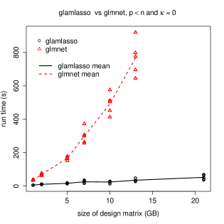
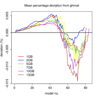
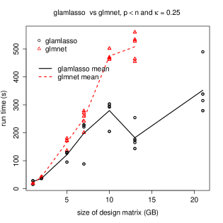
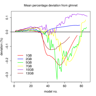
Figure 8: Benchmark results for the Gaussian models and $p<n$. Run time in seconds is shown as a function of the size of the design matrix in GB (left). Relative mean deviation in the attained objective function values as given by (20) is shown as a function of model number (right). The top row gives the results for $\kappa=0$ and the bottom for $\kappa=0.25$.

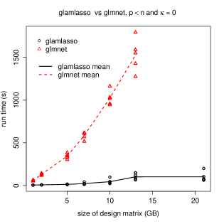
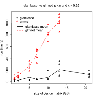
Figure 9: Benchmark results for the Poisson models and $p<n$. Run time in seconds is shown as a function of the size of the design matrix in GB (left). Relative mean deviation in the attained objective function values as given by (20) is shown as a function of model number (right). The top row gives the results for $\kappa=0$ and the bottom for $\kappa=0.25$.

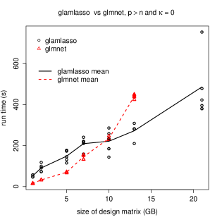
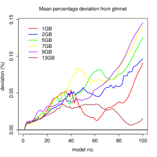
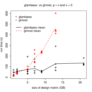
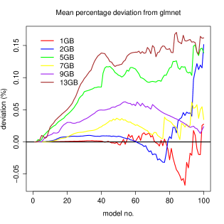
Figure 10: Benchmark results for $p>n$. Run time in seconds is shown as a function of the size of the design matrix in GB (left). Relative mean deviation in the attained objective function values as given by (20) is shown as a function of model number (right). The top row gives the results for the Gaussian model and the bottom for Poisson model.

Figure 8 shows the results for the Gaussian models for $p<n$. Here glamlasso generally outperformed glmnet in terms of run time – especially for $\kappa=0$. It scaled well with the size of the design matrix and it could fit the model for large design matrices that glmnet could not handle.

It should be noted that for the Gaussian models with the identity link there is no outer loop, hence the comparison is in this case effectively between the (GLAM enhanced) proximal gradient algorithm and the coordinate descent algorithm as implemented in glmnet.

Figure 9 shows the results for the Poisson models for $p<n$. As for the Guassian case, glamlasso was generally faster than glmnet. The run times for glamlasso also scaled very well with the size of the design matrix for both values of $\kappa$.

Figure 10 shows the results for both models for $p>n$ and $\kappa=0$. Here the run times were comparable for small design matrices, with glmnet being a little faster for the Gaussian model, but glamlasso stilled scaled better with the size of the design matrix. For $\kappa>0$ (results not shown) glamlasso retained its benefit in terms of memory usage, but glmnet became comparable or even faster for the Gaussian model than glamlasso.

In the comparisons above we have not included the time it took to construct the actual design matrix for the glmnet procedure. However, the construction and handling of matrices, whose size is a substantial fraction of the computers memory, was quite time consuming (between 15 minutes and up to one hour) underlining the advantage of our design matrix free method.

7 Discussion

The algorithm implemented in the R package glmnet and described in Friedman et al. (2010) computes the penalized and weighted least squares estimate given by (10) by a coordinate descent algorithm. For penalty functions like the 1-norm that induce sparsity of the minimizer, this is recognized as a very efficient algorithm. Our initial strategy was to adapt the coordinate descent algorithm to GLAMs so that it could take advantage of the tensor product structure of the design matrix. It turned out to be difficult to do that. It is straight forward to implement a memory efficient version of the coordinate descent algorithm that does not require the storage of the full tensor product design matrix, but it is not obvious how to exploit the array structure to reduce the computational complexity. Consequently, our implementation of such an algorithm was outperformed by glmnet in terms of run time, and for this reason alternatives to the coordinate descent algorithm were explored.

Proximal gradient algorithms for solving nonsmooth optimization problems have recently received renewed attention. One reason is that they have shown to be useful for large-scale data analysis problems, see e.g. Parikh and Boyd (2014). In the image analysis literature the proximal gradient algorithm for a squared error loss with an $\ell_{1}$-penalty is known as ISTA (iterative selection-thresholding algorithm), see Beck and Teboulle (2009) and Beck and Teboulle (2010). The accelerated version with a specific acceleration sequence was dubbed FISTA (fast ISTA) by Beck and Teboulle (2009). For small-scale problems and unstructured design matrices it is our experience that the coordinate descent algorithm outperforms accelerated proximal algorithms like FISTA. This observation is also in line with the more systematic comparisons presented in Section 5.5 in Hastie et al. (2015). For large-scale problems and/or structured design matrices – such as the tensor product design matrices considered in this paper – the proximal gradient algorithms may take advantage of the structure. The Gaussian smoothing example demonstrated that this is indeed the case.

When the squared error loss is replaced by the negative log-likelihood our proposal is similar to the approach taken in glmnet, where penalized weighted least squares problems are solved iteratively by an inner loop. The main difference is that we suggest using a proximal gradient algorithm instead of a coordinate descent algorithm for the inner loop. Including weights is only a trivial modification of FISTA from Beck and Teboulle (2009), but the weight matrix commonly used for fitting GLMs is not a tensor product. Despite of this it is still possible to exploit the tensor product structure to speed up the inner loop, but by making a tensor approximation to the weights we obtained in some cases further improvements. For this reason we developed the GD-PG algorithm with an arbitrary choice of weights. The Poisson smoothing example demonstrated that when compared to coordinate descent the inner PG loop was capable of taking advantage of the tensor product structure.

The convergence analysis combines general results from the optimization literature to obtain convergence results for the inner proximal algorithm and the outer gradient based descent algorithm. These results are strongest when the design matrix has rank $p$ (thus requiring $p\leq n$). Convergence for $p>n$ would require additional assumptions on $J$, which we have not explored in any detail. Our experience for $J=\|\cdot\|_{1}$ is that the algorithm converges in practice also when $p>n$. Our most important contribution to the convergence analysis is the computation of the upper bound $\hat{L}^{(k)}$ of the Lipschitz constant $L^{(k)}$. This upper bound relies on the tensor product structure. For large-scale problems the computation of $L^{(k)}$ will in general be infeasible due to the size of $X^{\top}W^{(k)}X$. However, for the tensor product design matrices considered, the upper bound is computable, and a permissible stepsize $\delta^{(k)}$ that ensures convergence of the inner PG loop can be chosen.

It should be noted that the GD-PG algorithm requires minimal assumptions on $J$, but that the proximal operator associated with $J$ should be fast to compute for the algorithm to be efficient. Though it has not been explored in this paper, the generality allows for the incorporation of convex parameter contraints. For box constraints $J$ will be separable and the proximal operator will be fast to compute.

The simulation study confirmed what the smoothing applications had showed, namely that the GD-PG algorithm with $J=\|\cdot\|_{1}$ and its implementation in the R package glamlasso scales well with the problem size. It can, in particular, efficiently handle problems where the design matrix becomes prohibitively large to be computed and stored explicitly. Moreover, in the simulation study the run times were in most cases smaller than or comparable to that of $\verb+glmnet+$ even for small problem sizes. However, the simulation study also revealed that when $p>n$ the run time benefits of $\verb+glamlasso+$ over $\verb+glmnet+$ were small or dimished completely – in particular for small problem sizes. One explanation could be that $\verb+glmnet+$ implements a screening rule, which is particularly beneficial when $p>n$. It appears to be difficult to combine such screening rules with the tensor product structure of the design matrix. When $p<n$, as in the smoothing applications, glamlasso was, however, faster than glmnet and scaled much better with the size of the problem. This was true even when a sparse representation of the design matrix was used, though glmnet was faster and scaled better with the size of the design matrix in this case for both examples. It should be noted that glamlasso achieves its performance without relying on sparsity of the design matrix, and it thus works equally well for smoothing with non-local as well as local basis functions.

In conclusion, we have developed and implemented an algorithm for computing the penalized maximum likelihood estimate for a GLAM. When compared to Currie et al. (2006) our focus has been on nonsmooth penalty functions that yield sparse estimates. It was shown how the proposed GD-PG algorithm can take advantage of the GLAM data structure, and it was demonstrated that our implementation is both time and memory efficient. The smoothing examples illustrated how GLAMs can easily be fitted to 3D data on a standard laptop computer using the R package glamlasso.

8 Supplementary Materials

SuppMatJCGS

SuppMatJCGS is a folder containing scripts and datasets used in the examples in sections 4.2.1, 4.2.2, 4.3 and 6.5 along with a ReadMe file. (SuppMatJCGS.zip, zipped file).

Appendix A The maps $\operatorname{vec}$ and $\rho$

The map $\operatorname{vec}$ maps an $n_{1}\times\ldots\times n_{d}$ array to a $\prod_{i=1}^{d}n_{d}$-dimensional vector. This is sometimes known as “flattening” the array. For $j=1,\ldots,d$ and $i_{j}=1,\ldots,n_{j}$ introduce the integer

$$[i_{1},\ldots,i_{d}]\coloneqq i_{1}+n_{1}((i_{2}-1)+n_{2}((i_{3}-1)+\ldots n_{d-1}(i_{d}-1)\ldots)).$$ (48)

Then $\operatorname{vec}$ is defined as

$$\operatorname{vec}(A)_{[i_{1},\ldots,i_{d}]}\coloneqq A_{i_{1},\ldots,i_{d}}$$ (49)

for an array $A$. This definition of $\operatorname{vec}$ corresponds to flattening a matrix in column-major order.

Following the definitions in Currie et al. (2006) (see also De Boor (1979) and Buis and Dyksen (1996)), $\rho$ maps an $r\times n_{1}$ matrix and an $n_{1}\times\ldots\times n_{d}$ array to an $n_{2}\times\ldots\times n_{d}\times r$ array. With $X$ the matrix and $A$ the array then

$$\rho(X,A)_{i_{1},\ldots,i_{d}}\coloneqq\sum_{j}X_{i_{d},j}A_{j,i_{1},\ldots,i_{d-1}}.$$ (50)

From this definition it follows directly that

$$(X_{d}\otimes\ldots\otimes X_{1})\operatorname{vec}(A)_{[i_{1},\ldots,i_{d}]} =\sum_{j_{1},\ldots,j_{d}}X_{d,i_{d},j_{d}}\cdots X_{1,i_{1},j_{1}}A_{j_{1},\ldots,j_{d}}$$

$$=\sum_{j_{d}}X_{d,i_{d},j_{d}}\cdots\sum_{j_{2}}X_{2,i_{2},j_{2}}\sum_{j_{1}}X_{1,i_{1},j_{1}}A_{j_{1},\ldots,j_{d}}$$

$$=\rho(X_{d},\ldots,\rho(X_{2},\rho(X_{1},A))\ldots)_{i_{1},\ldots,i_{d}}$$

where $[i_{1},\ldots,i_{d}]$ denotes the index defined by (48).

Appendix B Exponential families

The exponential families considered are distributions on $\mathbb{R}$ whose density is

$$f_{\vartheta,\psi}(y)=\exp\Big{(}\frac{a(\vartheta y-b(\vartheta))}{\psi}\Big{)}$$

w.r.t. some reference measure. Here $\vartheta$ is the canonical (real valued) parameter, $\psi>0$ is the dispersion parameter, $a>0$ is a known and fixed weight and $b$ is the log-normalization constant as a function of $\vartheta$ that ensures that the density integrates to 1. In general, $\vartheta$ may have to be restricted to an interval depending on the reference measure used. Note that the reference measure will depend upon $\psi$ but not on $\vartheta$.

With $\eta$ denoting the linear predictor in a generalized linear model we regard $\vartheta(\eta)$ as a parameter function that maps the linear predictor to the canonical parameter, such that the mean equals $g^{-1}(\eta)$ when $g$ is the link function. From this it can easily be derived that $b^{\prime}(\vartheta(\eta))=g^{-1}(\eta)$. For a canonical link function, $\vartheta(\eta)=\eta$ and $b^{\prime}=g^{-1}$. In terms of $\eta$ the log-density can be written as

$$\log f_{\vartheta(\eta),\psi}(y)\propto a(\vartheta(\eta)y-b(\vartheta(\eta))).$$

From this it follows that

$$\partial_{\eta}\log f_{\vartheta(\eta),\psi}(y)=a\vartheta^{\prime}(\eta)(y-g^{-1}(\eta)),$$ (51)

and the score statistic, $u=\nabla_{\eta}l(\eta)$, entering in (4) is thus given by

$$u_{i}=a_{i}\vartheta^{\prime}(\eta_{i})(y_{i}-g^{-1}(\eta_{i})),\quad i=1,\ldots n.$$ (52)

The weights commonly used when fitting a GLM are

$$w_{i}=\vartheta^{\prime}(\eta_{i})(g^{-1})^{\prime}(\eta_{i}),$$ (53)

which are known to be strictly positive provided that $(g^{-1})^{\prime}$ is nonzero everywhere (thus $g^{-1}$ is strictly monotone). This is not entirely obvious, but $w_{i}$ is the variance of $u_{i}$ (with $a_{i}=1$ and $\psi=1$), which is nonzero whenever $(g^{-1})^{\prime}$ is nonzero everywhere.

We may note that when the weights are given by (53), the working response $z$, see (9), given the linear predictor $\eta$ can be computed as

$$z_{i}=a_{i}(y_{i}-g^{-1}(\eta_{i}))g^{\prime}(g^{-1}(\eta_{i}))+\eta_{i},$$ (54)

which renders it unnecessary to compute the intermediate score statistic.

References

- Bapat (2010) Bapat, R. (2010). Graphs and Matrices. Universitext. Springer.
- Beck and Teboulle (2009) Beck, A. and M. Teboulle (2009). A fast iterative shrinkage-thresholding algorithm for linear inverse problems. SIAM Journal on Imaging Sciences 2(1), 183–202.
- Beck and Teboulle (2010) Beck, A. and M. Teboulle (2010). Gradient-based algorithms with applications to signal recovery problems. In D. P. Palomar and Y. C. Eldar (Eds.), Convex Optimization in Signal Processing and Communications, pp. 3–51. Cambridge University Press.
- Bühlmann and van de Geer (2011) Bühlmann, P. and S. van de Geer (2011). Statistics for High-Dimensional Data: Methods, Theory and Applications. Springer Series in Statistics. Springer Berlin Heidelberg.
- Buis and Dyksen (1996) Buis, P. E. and W. R. Dyksen (1996). Efficient vector and parallel manipulation of tensor products. ACM Transactions on Mathematical Software (TOMS) 22(1), 18–23.
- Currie et al. (2006) Currie, I. D., M. Durban, and P. H. Eilers (2006). Generalized linear array models with applications to multidimensional smoothing. Journal of the Royal Statistical Society: Series B (Statistical Methodology) 68(2), 259–280.
- De Boor (1979) De Boor, C. (1979). Efficient computer manipulation of tensor products. ACM Transactions on Mathematical Software (TOMS) 5(2), 173–182.
- Eddelbuettel and François (2011) Eddelbuettel, D. and R. François (2011). Rcpp: Seamless R and C++ integration. Journal of Statistical Software 40(8), 1–18.
- Friedman et al. (2010) Friedman, J., T. Hastie, and R. Tibshirani (2010). Regularization paths for generalized linear models via coordinate descent. Journal of statistical software 33(1), 1.
- Hastie et al. (2015) Hastie, T., R. Tibshirani, and M. Wainwright (2015). Statistical Learning with Sparsity: The Lasso and Generalizations. Chapman & Hall/CRC Monographs on Statistics & Applied Probability. CRC Press.
- Horn and Johnson (1991) Horn, R. A. and C. R. Johnson (1991). Topics in Matrix Analysis. Cambridge University Press.
- Lund (2016) Lund, A. (2016). glamlasso: Penalization in large scale generalized linear array models.
- Moreau (1962) Moreau, J.-J. (1962). Fonctions convexes duales et points proximaux dans un espace hilbertian. C. R. Acad. Sci., Paris 255, 2897–2899.
- Nelder and Wedderburn (1972) Nelder, J. A. and R. W. M. Wedderburn (1972). Generalized linear models. Journal of the Royal Statistical Society: Series A (General) 135(3), 370–384.
- Parikh and Boyd (2014) Parikh, N. and S. Boyd (2014). Proximal algorithms. Foundations and Trends® in Optimization 1(3), 127–239.
- Roland et al. (2006) Roland, P. E., A. Hanazawa, C. Undeman, D. Eriksson, T. Tompa, H. Nakamura, S. Valentiniene, and B. Ahmed (2006). Cortical feedback depolarization waves: A mechanism of top-down influence on early visual areas. Proceedings of the National Academy of Sciences 103(33), 12586–12591.
- Springer and Thompson (1970) Springer, M. D. and W. E. Thompson (1970). The distribution of products of beta, gamma and gaussian random variables. SIAM Journal on Applied Mathematics 18(4), pp. 721–737.
- Tseng and Yun (2009) Tseng, P. and S. Yun (2009). A coordinate gradient descent method for nonsmooth separable minimization. Mathematical Programming 117(1-2), 387–423.
- Vincent et al. (2014) Vincent, M., Hansen, and N. R. (2014). Sparse group lasso and high dimensional multinomial classification. Computational Statistics & Data Analysis 71, 771–786.
- Wood (2006) Wood, S. (2006). Generalized Additive Models: An Introduction with R. Chapman & Hall/CRC Texts in Statistical Science. Taylor & Francis.
- Zhang et al. (2013) Zhang, H., J. Jiang, and Z.-Q. Luo (2013). On the linear convergence of a proximal gradient method for a class of nonsmooth convex minimization problems. Journal of the Operations Research Society of China 1(2), 163–186.
- Zou and Li (2008) Zou, H. and R. Li (2008). One-step sparse estimates in nonconcave penalized likelihood models. Annals of statistics 36(4), 1509.