Resonance-inclined optical nuclear spin polarization of liquids in diamond structures

Abstract

Dynamic nuclear polarization (DNP) of molecules in a solution at room temperature has potential to revolutionize nuclear magnetic resonance spectroscopy and imaging. The prevalent methods for achieving DNP in solutions are typically most effective in the regime of small interaction correlation times between the electron and nuclear spins, limiting the size of accessible molecules. To solve this limitation, we design a mechanism for DNP in the liquid phase that is applicable for large interaction correlation times. Importantly, while this mechanism makes use of a resonance condition similar to solid-state DNP, the polarization transfer is robust to a relatively large detuning from the resonance due to molecular motion. We combine this scheme with optically polarized nitrogen vacancy (NV) center spins in nanodiamonds to design a setup that employs optical pumping and is therefore not limited by room temperature electron thermal polarisation. We illustrate numerically the effectiveness of the model in a flow cell containing nanodiamonds immobilized in a hydrogel, polarising flowing water molecules 4700-fold above thermal polarisation in a magnetic field of 0.35 T, in volumes detectable by current NMR scanners.

Introduction: Nuclear spin hyperpolarization, i.e. a population difference between the nuclear spin states that exceeds significantly the thermal equilibrium value, is a key emerging method for increasing the sensitivity of nuclear magnetic resonance (NMR) Bloch ; Bloch2 which is proportional to the sample polarisation. By enhancing the magnetic resonance signals by several orders of magnitude, a wide range of novel applications in biomedical sciences are made possible, such as metabolic MR imaging law2002high or characterization of molecular chemical composition luchinat2008nuclear ; bertini2005nmr . Dynamic nuclear polarization (DNP), by which electron spin polarization is transferred to nuclear spins, is one of the promising methods to reach such a large enhancement of the signal. Nuclear spin hyperpolarization, i.e. a population difference between the nuclear spin states that exceeds significantly the thermal equilibrium value, is a key emerging method for increasing the sensitivity of nuclear magnetic resonance (NMR) Bloch ; Bloch2 which is proportional to the sample polarisation. By enhancing the magnetic resonance signals by several orders of magnitude, a wide range of novel applications in biomedical sciences are made possible, such as metabolic MR imaging law2002high or characterization of molecular chemical composition luchinat2008nuclear ; bertini2005nmr . Dynamic nuclear polarization (DNP), by which strong electron spin polarization is transferred to nuclear spins, is one of the promising methods to reach such a large enhancement of the signal. Over the past decades, one of the outstanding challenges is the hyperpolarization of molecules in a solution nesmelov2004aqueous ; abragam ; mccarney2008spin1 ; mccarney2008spin2 ; ebert2012mobile ; anderson1962influence ; Gabl . In typical solutions, resonance-based polarization mechanisms commonly used in solid-state systems abragam1978 ; wenckebach2008solid are not effective due to the averaging of the electron-nuclear anisotropic interaction of the molecules by their rapid motion. Thus, cross-relaxation mechanisms such as the Overhauser effect abragam ; anderson1962influence ; Gabl are typically applied to realise polarization of fluids under ambient conditions. So far, the largest hyperpolarization is achieved for fast diffusing small molecules and is severely limited by the low thermal electron polarization in moderate magnetic fields. For example, for TEMPO, trityl or biradical systems, the electron spin polarisation amounts to only 0.08% percent for a magnetic field of $B=0.36$ T mccarney2008spin1 ; mccarney2008spin2 .

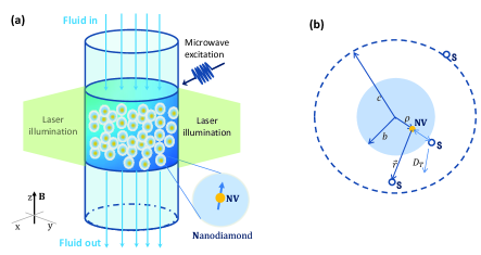
Figure 1: (a) Schematics of the setup for polarisation of nuclear spin in solution via NV centers in nanodiamonds. Water is pumped into a channel containing a hydrogel cell with the immobilized nanodiamonds for continuous DNP polarisation. Laser illumination is used for polarising the NV spins and WM irradiation facilitates the transfer to nuclear spins in surrounding molecules. The hyperpolarized water then flows downstream for NMR detection. A permanent magnetic field $B$ is applied along the $z$-axis, which defines the coordinate system. (b) Illustration of the model parameters.

In this work, we demonstrate that the use of optically hyperpolarized electron spins offers an exciting possibility for overcoming the limitation on the degree and rate of electron polarization. Specifically, nitrogen vacancy (NV) centers in nanodiamonds make an excellent candidate as optically pumped hyperpolarisation agents. The unique optical properties of the negatively charged nitrogen-vacancy center in nanodiamonds allow for over 90% electron spin polarization to be achieved in less than a microsecond by optical pumping Manson2006 while exhibiting a relaxation time in the millisecond range even at room temperature jelezko . Methods for the creation of high polarization in ${}^{13}C$ nuclear spins inside of bulk diamond have already been developed theoretically and demonstrated experimentally chen ; Cai ; Cai2 ; CaiRJP13 ; London ; King ; Bretschneider .

However, for NV centers the interaction correlation time $\tau_{c}$ with nuclear spins in surrounding molecules is atypically large, as $\tau_{c}$ scales with the square of the minimum distance with the nuclear spins, which is very large (a few nanometers) for NV centers in nanodiamonds. Thus, NV centers cannot typically be used with standard Overhauser cross-relaxation protocols. Here, we present a new theoretical framework for polarizing molecules for systems with a large correlation time. Specifically, we apply resonance-based schemes, such as the solid effect, where under continuous microwave (MW) radiation the electron spin is driven to approach resonance with the nuclear spin of choice. Importantly, we will proceed to demonstrate that this scheme remains robust even in the presence of molecular motion and, unlike solid-state polarization methods, is tolerant to a relative large detuning from the resonance frequency.

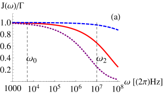
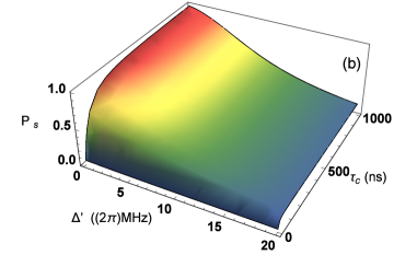
Figure 2: (a) Spectra density function $J(\omega)$ as a function of frequency $\omega$ and interaction correlation time $\tau_{c}$ . The blue dashed, red solid, and purple dotted lines correspond to $\tau_{c}=0.1$ ns, 10 ns and 100 ns respectively. (b) The steady-state polarization of the nuclear spins. $\omega_{S}=(2\pi)16$ MHz, $\epsilon_{0}=\Omega=(2\pi)8\sqrt{2}$ MHz, and $\Delta^{\prime}=\epsilon(\theta)-\epsilon_{0}$ is the detuning from the resonance point.

We then proceed to consider a specific setup that allows to realise this protocol, where the nanodiamonds are immobilized in a hydrogel inside a flow channel, increasing $\tau_{c}$, as well as limiting the nuclear spin relaxation due to electron spins to the polarization region. Due to the optical NV polarization, and the efficiency of our scheme in the large $\tau_{c}$ regime, a very high nuclear spin polarization is achieved for volumes that are detectable in current NMR scanners.

Spin polarisation via resonance-inclined transfer (SPRINT) – We consider the polarization transfer induced by magnetic dipole-dipole coupling between an electron spin and all the surrounding solvent spins. Suppose as shown in Fig. 1(a) that the electron spin is located in the center of a nanoparticle, assuming the radius of the small solvent molecule to be negligible, the distance of closest approach of the electron and nuclear spins, $b$, coincides with the radius of the nanoparticle. All the solvent molecules are diffusing in a solution with the translational diffusion coefficient $D_{T}$. The interaction between electron and solvent spins evolves in time with a characteristic correlation time $\tau_{c}=b^{2}/D_{T}$. $c$ and $\rho$ in Fig. 1(b) are related to absorbing boundary and off-center effect, respectively, which are negligible in our case, see supplementary information (SI) SI .

In resonance-based DNP schemes, continuous MW radiation is applied to the electron spin abragam1978 ; wenckebach2008solid , thus creating an “effective frequency” of the electron spin $\omega_{E}$ in the rotating frame. When the energy difference between the effective frequency and the Larmor frequency $\omega_{S}$ of a specific nuclear spin species vanishes ($\omega_{0}=\omega_{E}-\omega_{S}\rightarrow 0$) a Hartmann-Hahn (H-H) resonance is achieved Hartman ) and energy-conserving flip-flop transitions can occur between the electron and nuclear spins. Energy non-conserving flip-flip transitions are suppressed due to large energy mismatch compared with the effective coupling between the electron and nuclear spin ($\omega_{2}=\omega_{E}+\omega_{S}\gg g$). This difference between the flip-flop and flip-flip transitions leads to a net polarization transfer from electron spins to nuclear spins SI ; Solomon .

However, in the liquid phase, due to fast molecular diffusion, the nuclear spins interact with the electron spin within a finite correlation time $\tau_{c}$. Perturbatively, we calculate the transition probabilities $W_{i}$ ($i=0,2$) of the flip-flop transition rate $W_{0}=\alpha_{0}J(\omega_{0})$ and flip-flip transition rate $W_{2}=\alpha_{0}J(\omega_{2})$, in which the spectral density function is given by hwang ; Halle ; SI ,

$$J(\omega) = \Gamma Re\Big{[}\frac{1+\frac{\sqrt{i\xi}}{4}}{1+\sqrt{i\xi}+\frac{4(\sqrt{i\xi})^{2}}{9}+\frac{(\sqrt{i\xi})^{3}}{9}}\Big{]}$$ (1)

where $\xi=\omega\tau_{c}$ with $\omega$ the relevant energy frequency (e.g. $\omega_{0}$ or $\omega_{2}$). $\alpha_{0}$ is a constant involving the nuclear properties of the interacting system. $\Gamma$ is the coefficient determined by system parameters, such as minimum distance between the electron and solvent spins, dipole-dipole coupling strength and translational diffusion coefficient etc (see the SI SI for details). In simple solvents of low viscosity such as protons in free water molecules $D_{T}=D_{w}=2\times 10^{-9}$ $m^{2}/s$ Krynicki and for a minimal distance of the electron and solvent spins of $b=0.5$ nm we find $\tau_{c}=b^{2}/D_{T}\sim 0.1$ ns. Then $\xi\ll 1$ is always satisfied for weak and moderate magnetic fields (i.e. $B<1$ T) resulting in $\omega_{S}=(2\pi)16$ MHz for $B=0.36$ T as shown by the blue dashed line in Fig. 2(a). Applying a MW driving fulfilling $\omega_{E}=\omega_{S}$ will lead to no appreciable difference between flip-flip and flip-flop effects, as $J\left(\omega_{2}\right)\cong J\left(\omega_{0}\right)\cong J(0)$ in general. This indifference of the transition rates to the energy mismatch is the main reason why resonance-based polarization schemes are not applicable to solutions with small $\tau_{c}$. However, larger interaction correlation times achieved by increasing the distance $b=5$ nm and decreasing the diffusion coefficient $D_{T}=10D_{w}$ to induce $\tau_{c}=100$ ns, as shown in the purple dotted line in Fig. 2(a)), demonstrate a clear incline of net polariation towards resonance condition. Using the same parameters discussed above, we now obtain $J(\omega_{0})=J(0)\sim 1$ and $J(\omega_{2})\sim 0$. Therefore, it is possible to achieve a polarization transfer in solution with large $\tau_{c}$ by matching a H-H resonant condition. It is interesting to note that the relationship between our scheme and standard Overhauser cross-polarisation is similar to the sideband resolved regime and the Doppler (unresolved) regime in laser cooling of cold trapped ions (see SI SI ). This results in a more efficient polarisation transfer, which enables DNP via more distant electron spins, and with a weaker dipolar coupling to the nuclear spins.

The steady state populations in the different nuclear spin states and the resulting polarization can then be determined from a detailed balance analysis. We find (we ignore here relaxation times, see SI SI for a more detailed treatment)

$$P_{s} = -\frac{J(\omega_{0})-J(\omega_{2})}{J(\omega_{0})+C_{0}J(\omega_{S})+J(\omega_{2})},$$ (2)

in which $C_{0}=2\cot\varphi$ with $\cot\varphi=\epsilon/\Omega$ depending on the Rabi frequency of the MW radiation $\Omega$ and detuning of the MW field from the electron energy scale $\epsilon$. Here we assume that the electron spin is continuously pumped into a polarized state. Fig. 2(b) shows the dependence of the achieved steady-state polarization on the detuning from the resonance condition and correlation time. As we are using the solid effect, we tune the MW field to achieve resonant interaction as $\omega_{S}=\sqrt{\epsilon^{2}+\Omega^{2}}=\omega_{E}=(2\pi)16$ MHz (see SI SI ), where we have chosen $\epsilon=\Omega=(2\pi)8\sqrt{2}$ MHz. As shown in Fig. 2 (a), for a large correlation time satisfying $\tau_{c}>10$ ns, different rates between the flip-flop and flip-flip transitions induce a high steady-state polarization, quite similar to solid-state mechanisms. However, contrary to the solid-state phase, we can see that high steady-state polarization is achieved for a wide range of detuning from the resonance, as shown in Fig. 2(b). For example, for $\tau_{c}=100$ ns, we observe a high steady-state polarization for a detuning as large as $\Delta^{\prime}\sim(2\pi)10$ MHz. This is a unique characteristic of our theory in the liquid phase and different from the solid-phase in which polarization transfer only occurs when the detuning is comparable or smaller than the effective collective flip-flop coupling between the electron spin and nuclear spins chen ; London . Thus, this polarization by cross-relaxation requires an inclination towards resonance, but the resonance condition does not have to be matched exactly.

Optical SPRINT with nanodiamonds– To model the dynamics of nuclear spin polarization transfer from NV centers in nanodiamonds to the protons in water, we consider a setup of Fig. 1(a). The solvent spins of the target molecules are pumped through a flow cell containing a hyperpolarization region in which nanodiamonds are immobilized in a hydrogel layer (see Fig. 1), causing a dipolar magnetic interaction between the NV spins and their surrounding solvent spins with a characteristic correlation time $\tau_{c}$. Here the electron spins of the NV centers will be strongly polarized by optical pumping and the hydrogel provides a method for increasing the correlation time by reducing the diffusion rate of water molecules by a factor of $10^{2}-10^{3}$ via controlling the mesh sizes and types of hydrogels Shapiro .

A DC magnetic field $B\cong 0.36$ T whose direction defines the z-axis of the laboratory frame is applied to the system. We assume $\gamma_{e}B\gg D$ where $\gamma_{e}B$ denotes the NV centre Larmor frequency and $D$ its zero-field splitting. As discussed in Ref. chen , in this regime the quantisation axis of all NV centres is along the magnetic field direction, and the orientation of the symmetry axis of the NV center relative to the external magnetic field is uniformly distributed over the unit sphere. Here $\theta$ denotes the angle between the NV center symmetry axis and the magnetic field axis. The random orientations of the NV centers causes two difficulties for the polarization transfer from the NV spin to the nuclear spins. First, high optical polarization of the NV center spins is only achieved for the NV orientation near $\theta=0^{\circ}$ and $\theta=90^{\circ}$ by using 532 nm green laser illumination and, secondly, there’s a variation of the energy splitting with $\theta$ (see SI SI ).

The rate of the polarization transfer is given by $W=W_{0}-W_{2}=\alpha_{0}(J(\omega_{0})-J(\omega_{2}))$ SI . Assuming the magnetic field is given by $B=0.36$ T, $\omega_{S}=(2\pi)16$ MHz, for utilizing the effect of resonance in the current setup, we tune the MW frequency to achieve resonant interaction for $\theta=90^{\circ}$, and $\varepsilon_{0}=\varepsilon(90^{\circ})=\Omega=(2\pi)8\sqrt{2}$ MHz for matching a H-H resonance. Due to the strong dependence of the energy splitting between the spin levels on $\theta$, for each NV spin with a specific $\epsilon(\theta)$, there is a detuning from resonance which leads to $\Delta^{\prime}$ in Fig. 2(b). The reason that we focus here on the near resonant case around $\theta=90^{\circ}$ can be found in the observation that the same detuning leads to more NV spins to be involved in the $\theta=90^{\circ}$ case as compared to the $\theta=0^{\circ}$ case (e.g. $\Delta^{\prime}<(2\pi)10$ MHz involves 5% NV spins in nanodiamonds in the former as compared to just 0.1% NV spins for the latter chen . We estimate the efficiency of our scheme by calculating the average polarization rate of the solvent spins $\overline{W}_{eff}=S^{-1}\int_{S}WP_{C}\cos\varphi dS$, in which $P_{C}\cos\varphi$ is the initial polarization of the corresponding NV spin according to the solid effect polarization mechanism wenckebach2008solid and $S$ is the solid angle covered.

Consider continuous optical pumping as well as optical initialization of the NV spins for $\theta=90^{\circ}$, where $P_{C}\simeq 0.5^{2}=0.25$. The dependence of the average polarization rate of the solvent spins for nanodiamonds of $b=5$nm radius on the ratio of the decreased translational diffusion $k$ is shown in Fig. 3. Slow translational diffusion of the solvent molecules affects the polarization transfer in two competing ways: (i) increasing the correlation time to enhance the polarization transfer and (ii) decreasing the number of the involved NV spins contributing to the polarization transfer (as slower diffusion leads to smaller accessible detuning from resonance for our scheme). Fig. 3 predicts that the former will dominate (as expected, since the first effect is linear and the second sub-linear). Thus, a fast polarization transfer can be achieved via a decrease of the diffusion rate. For example, when the size of the nanodiamond is $b=5$ nm, $\overline{W}_{eff}\approx 0.04$ ms^-1 for $k=1$ and $\overline{W}_{eff}\approx 1.4$ ms^-1 for $k=100$.

The proposed setup is feasible with current experimental technology. Over the past decade, several experiments have realised polarization of flowing solvents by immobilized electron spins such as TEMPO and radicals in hydrogel layers mccarney2008spin1 ; mccarney2008spin2 ; ebert2012mobile for $B\simeq 0.35$ T. Furthermore, it has been demonstrated that one can use functional groups on the diamond surface to replace these radicals with nanodiamonds in the hydrogel HuangH ; Haartman . The nanodiamonds are immobilized in the hydrogel and it is not necessary to consider rotational diffusion. While the implementations employing either radicals or nanodiamonds are similar in spirit, it is crucial that the transparency of the hydrogel allows for the optical polarization of nanodiamonds which has the potential to lead to a 300-fold increase of the achievable nuclear polarisation over the implementations using radicals.

To estimate the total polarization of the solvent spins, we use an approximate formula for the steady state bulk nuclear spin polarization of the solvent neglecting polarization diffusion,

$$P_{lim} \approx \frac{N_{e}}{N_{p}}\overline{W}_{eff}T_{p}.$$ (3)

Here $\frac{N_{e}}{N_{p}}$ is the ratio of the number of the NV spins to proton spins in the polarization region (see SI SI ), and $T_{p}$ is the smaller one of the times that the solvent contacting time with the hydrogel matrix or the solvent relaxation time. Suppose the flow channel is composed of a tube of a diameter of 1 mm, the size of the hydrogel layer is 1 mm and the resulting volume is filled with nanodiamonds of 10nm diameter such that they account for 12% of the total volume. Assuming $k=100$, we choose the flow rate such that a molecule of water passes through the hydrogel layer in 1 second, so that $T_{p}\sim T_{1}\sim 1s$, namely $v=10^{-3}$ m/s (this low flow rate is easily produced via commercial pumps, and negligibly affects the molecular dynamics within $\tau_{c}$). Given the density of protons in free water $\frac{200}{3}$ nm^-3, we obtain $N_{e}/N_{p}\sim 4\times 10^{-6}$, $\overline{W}_{eff}\approx 1.4$ ms^-1, $T_{p}\approx 1$ s to arrive at a polarisation of $P_{lim}\approx 0.6\%$ for the solution. This polarization, achieved for a volume of $1\mu l$ in 1s is roughly $4700$ times the thermal polarization and would already suffice for detection in a commercial NMR scanner. It is interesting to note that a recently proposed setup for polarization of fluids in a microfluidic diamond channel achieves similar degree of polarization, but due to the limitations on the microfluidic channel size in the proposed protocol, it requires over $1000$ parallel channels for polarizing 1$\mu$l of solvent within 1 second Abrams .

The volume of optimally polarized fluid that can be generated per unit time in a flow channel largely depends on the thickness of the hydrogel layer, as faster flow velocities for thicker layers are easily accessible (to maintain $T_{p}\sim T_{1}$). One of the limitation in our setup is the laser intensity required to optically polarize the NV centre spins within 10-100 $\mu$s. Experiments performed in bulk diamond have shown that typically available lasers are sufficient for efficiently polarizing NV centers in 1 mm³ volume, though optical absorption by the NV centers would limit the efficient optical polarization for $>1$ mm thickness. Furthermore, due to the small nanodiamond radius, Mie scattering does not limit the optical penetration depth in the 1 mm volume for the nanodiamond concentration in the proposed setup SI , and consider a flow rate of 1mm/s, the temperature increases due to heating is expected to be limited to only a few degrees. A more stringent limitation on the channel diameter comes from the microwave attenuation. 1 mm diameter capillaries are typically used for solutions due to the microwave absorption by water, which limits the microwave power for larger channels nesmelov2004aqueous . Another important factor for the polarization transfer is the relaxation time $T_{1}$ of the protons in the hydrogel layer, as discussed in Ref. Shapiro , this would depend on the material and mesh size of the gel, but can be assumed to be 0.3-2s.

Figure 3: The averaged polarization rate of the solvent spins $\overline{W}_{eff}$. $b=5$ nm ND radius was assumed. $k=D_{w}/D_{T}$ with $D_{w}=2\times 10^{-9}$ $m^{2}/s$ the diffusion coefficient in free water at room temperature and $D_{T}$ is the decreased translational diffusion coefficient. The percent of involved NV spins accounting for 90% of the polarization transfer is given for three different points.

While we have demonstrated theoretically that our setup in combination with SPRINT can achieve significant hyperpolarization of water, we would like to stress that a wide variety of molecules can be polarized with the same methodology, including those with nuclear spin species different from hydrogen. Of particular interest here are ${}^{13}C$ nuclear spins for example in ${}^{13}C$ pyruvic acid or ${}^{13}C$ glucose which have applications in biomedical imaging and can be polarized via the same setup. The decrease in polarization rate due to the fact that the gyromagnetic ratio of carbon is four times smaller than that of protons is typically offset by the longer nuclear spin relaxation time. Larger molecules could also potentially be polarized in our setup, especially as the interaction correlation time with these molecules is naturally longer. In this scenario the properties of the hydrogel would have to be tuned to avoid a dramatic reduction of the molecules’ diffusion coefficient.

SPRINT can potentially be very effective for non-optical DNP systems, not involving nanodiamonds, for example for DNP in high magnetic fields and/or with biomacromolecules (e.g. proteins). In these systems, if the interaction correlation time between the polarizing electron (e.g. in a radical) and the molecule can be increased, it would be relatively straightforward to apply our scheme. We anticipate that with minor modifications, resonance-inclined transfer could be applied in combination with other solid-phase schemes such as the cross effect.

Conclusion – We developed SPRINT, a resonance-inclined mechanism for the polarization of nuclear spins for large interaction correlation times in a solution. Importantly, this is a complementary method to the Overhauser effect which is most efficient in the extreme narrowing regime. Due to molecular motion, our scheme is tolerant to a relatively large deviation from the resonant frequency. Furthermore, we propose a polarization setup using NV centres in nanodiamonds held in a hydrogel inside a flow cell which combines the advantages of this scheme with optical electron polarization. Under realistic experimental conditions, a polarization enhancment of 4700 times is observed. Finally, we predict that our resonance-inclined scheme could be used in a wide variety of DNP realizations, especially with biomacromolecules or in large magnetic fields.

Acknowledgements – We thank Yuzhou Wu, Pelayo Fernandez Acebal, Oded Rosolio and Martin Bruderer for the insightful discussions. This work was supported by an Alexander von Humboldt professorship, the ERC Synergy Grant BioQ, the ERC POC grant NDI, an IQST PhD Fellowship, the EU projects SIQS, DIADEMS and HYPERDIAMOND as well as the DFG CRC TR 21.

Supplementary Information to the manuscript
“Resonance-inclined optical nuclear spin polarization of liquids in diamond structures”

.1 Mechanism

.1.1 Basic Hamiltonian

For illustration of the basic idea, let us first consider a general system that is composed of an immobilized electron spin $1/2$ (notice that the NV spin $S=1$ could be simplified to be a two-level system which we will discuss later) and all its nearby diffusing solvent spins $I=1/2$. The Hamiltonian for such a system is then

$$H = \omega_{0s}\sigma_{z}+2\Omega(\cos\omega_{dr}t)\sigma_{x}+\sum_{n=0}^{N_{p}}\gamma_{n}BI^{n}_{z}+\sum_{n=0}^{N_{p}}g_{n}\Big{[}\vec{\sigma}\vec{I^{n}}-3(\vec{\sigma}\cdot\vec{e}_{nr})(\vec{I^{n}}\cdot\vec{e}_{nr})\Big{]},$$ (S1)

in which $\omega_{0s}$ represents the Zeeman splitting of the electron spin and the last term is the magnetic dipole-dipole interaction between the electron and nuclear spin. The length dependant factor $g_{n}$ and orientation of the inter-spin vector $\vec{e}_{nr}$ is modulated by the translational diffusion coefficient $D_{T}$, the rotational diffusion coefficient of the electron spin is not considered due to its immobilization in our setup. $\omega_{dr}$ is the driving microwave field of frequency, $\Omega$ is the Rabi frequency and $\gamma_{n}$ are the nuclear gyromagnetic ratio. Assuming a point-dipole interaction, neglecting the contact term and moving to a frame rotating with the drive frequency, we obtain

$$H^{\prime} = \epsilon\sigma_{z}+\Omega\sigma_{x}+\sum_{n=0}^{N_{p}}(\sigma_{z}\cdot\mathbf{A_{n}}\cdot\vec{I}^{n}+\gamma_{n}BI^{n}_{z}),$$ (S2)

where $\epsilon=\omega_{0s}-\omega_{dr}$, $\mathbf{A_{n}}=g_{n}\sqrt{1+3(e^{z}_{nr})^{2}}\vec{h}_{n}=A_{n}\vec{h}_{n}$ is the hyperfine interaction tensor for the nuclear spin, with $g_{n}=\frac{\mu_{0}}{4\pi}\frac{\gamma_{e}\gamma_{n}}{r_{n}^{3}}$ with $r_{n}=|\vec{r_{n}}|$ denoting the distance from electron spin to a nuclear spin. $\vec{h}_{n}$ determined by $\vec{e}_{nr}$: $h^{x}_{n}=3e^{x}_{nr}e^{z}_{nr}/\sqrt{1+3(e^{z}_{nr})^{2}}$, $h^{y}_{n}=3e^{y}_{nr}e^{z}_{nr}/\sqrt{1+3(e^{z}_{nr})^{2}}$, and $h^{z}_{n}=(3(e^{z}_{nr})^{2}-1)/\sqrt{1+3(e^{z}_{nr})^{2}}$. We also define $e^{z}_{nr}=\cos\theta^{\prime}_{n}$, $e^{x}_{r}=\sin\theta^{\prime}_{n}\cos\varphi^{\prime}_{n}$ and $e^{z}_{nr}=\sin\theta^{\prime}_{n}\sin\varphi^{\prime}_{n}$. By redefining the parameters we get:

$$H_{B}=\omega_{E}\sigma_{\tilde{z}}+\sum_{n=0}^{N_{p}}[\omega_{S}I^{n}_{z^{\prime}}+(\sigma_{\tilde{x}}\sin\varphi+\sigma_{\tilde{z}}\cos\varphi)\cdot(a_{x^{\prime}_{n}}I^{n}_{x^{\prime}}+a_{z^{\prime}_{n}}I^{n}_{z^{\prime}})],$$ (S3)

in which $\omega_{S}=\gamma_{n}B$, the angle $\varphi$ and $\omega_{E}$ are determined by

$$\sin\varphi=\frac{\Omega}{\sqrt{\epsilon^{2}+\Omega^{2}}},\ \ \ \omega_{E}=\sqrt{\epsilon^{2}+\Omega^{2}},\ \ \ \omega_{E}\sigma_{\tilde{z}}=\Omega\sigma_{z}+\epsilon\sigma_{x}$$

with $a_{x^{\prime}_{n}}=3g\cos\theta^{\prime}_{n}\sin\theta^{\prime}_{n}e^{i\phi^{\prime}_{n}}$ and $a_{z^{\prime}}=g(3\cos^{2}\theta^{\prime}_{n}-1)/r_{n}^{3}$ in which $g=\frac{\mu_{0}\hbar\gamma_{e}\gamma_{n}}{4\pi}$. Note that we consider the regime where the electron frequency $\omega_{0s}$ is large enough to fulfill $\omega_{0s}\tau_{c}>1$, i.e. outside the so-called “extreme-narrowing” limit. This condition allows us to disregard fast-oscillating terms when applying the MW driving.

We can rewrite the Hamiltonian as

$$H^{\prime}_{B} = \omega_{E}\sigma_{\tilde{z}}+\sum_{n=0}^{N_{p}}\omega_{S}I^{n}_{z^{\prime}}+(\sigma_{\tilde{x}}\sin\varphi+\sigma_{\tilde{z}}\cos\varphi)\cdot[3g\sqrt{\frac{8\pi}{15}}Y^{1}_{2}(\theta^{\prime}_{n},\phi^{\prime}_{n})I^{n}_{x^{\prime}}+g\sqrt{\frac{16\pi}{5}}Y^{0}_{2}(\theta^{\prime}_{n},\phi^{\prime}_{n})I^{n}_{z^{\prime}}],$$ (S4)

with the spherical harmonics $Y^{1}_{2}(\theta^{\prime}_{n},\phi^{\prime}_{n})=-\frac{1}{2}\sqrt{\frac{15}{2\pi}}\cos\theta^{\prime}_{n}\sin\theta^{\prime}_{n}e^{i\phi^{\prime}_{n}}$ and $Y^{0}_{2}(\theta^{\prime}_{n},\phi^{\prime}_{n})=\frac{1}{4}\sqrt{\frac{5}{\pi}}(3\cos^{2}\theta^{\prime}_{n}-1)$. The Hartmann-Hann resonant condition is given by $\omega_{E}=\omega_{S}$.

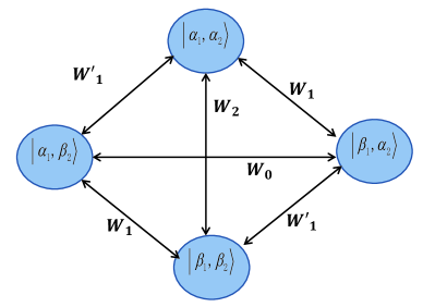
Figure S1: Transition probabilities between the eigenstates of the spin operators.

.1.2 Transition probability

In first order in perturbation theory the transition probability is given by $W_{ij}=\frac{1}{t}\bigg{\langle}|\int_{0}^{t}\langle i|H^{\prime}_{B}(t^{\prime})|j\rangle e^{i\omega_{ij}t^{\prime}}dt^{\prime}|^{2}\bigg{\rangle}_{noise}$ we readily arrive SolomonS

$$W_{ij} = \frac{1}{t}\bigg{\langle}\int_{0}^{t}\int_{0}^{t}\langle i|H^{\prime}_{B}(t^{\prime})|j\rangle\langle j|H^{\prime}_{B}(t^{\prime})|i\rangle e^{i\omega_{ij}(t^{\prime}-t^{\prime\prime})}dt^{\prime}dt^{\prime\prime}\bigg{\rangle}_{noise}$$

$$= \frac{1}{t}\int_{0}^{t}\int_{0}^{t}\bigg{\langle}\langle i|H^{\prime}_{B}(t^{\prime})|j\rangle\langle j|H^{\prime}_{B}(t^{\prime})|i\rangle\bigg{\rangle}_{noise}e^{i\omega_{ij}(t^{\prime}-t^{\prime\prime})}dt^{\prime}dt^{\prime\prime},$$

In principle this result is valid for short times as long as $e^{-W_{i}t}\ll 1,$ for longer times perturbation theory is invalid. However, this result is still valid for longer times in the limit $g\tau_{c}/r^{3}\ll 1$ and $t\gg\tau_{c}$, which is correct in the regime of this work. In this regime and in the assumption of Gaussian noise we get two integrals which are connected by the fluctuation dissipation theorem for which the imaginary part is just the power spectrum of the noise, or alternatively,

$$W_{i}(\omega_{i})=\alpha_{i}Re[\int_{-\infty}^{+\infty}G_{i}(t^{\prime})e^{i\omega_{i}t^{\prime}}dt^{\prime}]=\alpha_{i}J(\omega_{i}),$$ (S6)

in which $\alpha_{0}=\alpha_{2}=\frac{3\pi g^{2}\sin^{2}\varphi}{10}$, $\alpha_{1}=\frac{3\pi g^{2}\cos^{2}\varphi}{5}$, $\omega_{0}=\omega_{E}-\omega_{S}$, $\omega_{2}=\omega_{E}+\omega_{S}$ and $\omega_{1}=\omega_{S}$. All the related transitions are presented in Fig. S1, in which $|\alpha_{1}\rangle$, $|\beta_{1}\rangle$, $|\alpha_{2}\rangle$ and $|\beta_{2}\rangle$ are the eigenstates of electron and nuclear spins. $G_{i}(t^{\prime})$ is the space-dependent time-correlation function for dipolar interaction between spins NV and proton, which is expressed by

$$G_{i}(t^{\prime}) = \int\int N_{p}P(\vec{r_{0}})P(\vec{r_{0}}|\vec{r_{1}},t^{\prime})\frac{Y^{i}_{2}(\theta^{0},\phi^{0})Y^{i}_{2}(\theta^{1},\phi^{1})}{r_{0}^{3}r_{1}^{3}}d\vec{r_{0}}d\vec{r_{1}},$$

in which $i=0,1$ and $G_{2}(t^{\prime})=G_{0}(t^{\prime})$. Here $P(\vec{r_{0}})=1/V$ with the volume $V$. $P(\vec{r_{0}}|\vec{r_{1}},t^{\prime})$ is the well-known solution of the diffusion equation. As shown in Eq. (S6), the spectral density function is the real part of the Fourier-Laplace transform of the corresponding time autocorrelation function. Consider the diffusion coefficient $D_{T}$ in the whole space, one has Freed ; HalleS

$$J(\omega) = \Gamma Re\Bigg{[}\frac{1+\frac{\sqrt{i\xi}}{4}}{1+\sqrt{i\xi}+\frac{4(\sqrt{i\xi})^{2}}{9}+\frac{(\sqrt{i\xi})^{3}}{9}}\Bigg{]},$$ (S7)

in which the coefficient $\Gamma=\frac{8n_{p}}{27D_{T}b}$. Here $n_{p}$ is the proton number density, $D_{T}$ is the translational diffusion coefficient in hydrogel, $b$ is the closest distance between NV center and protons, and

$$\xi=\frac{\omega b^{2}}{D_{T}}=\omega\tau_{c}.$$

It is interesting to know, the principle part of this integral will induce a two body shift: $(\sigma_{z}+1)(\sigma_{z}-1)+(\sigma_{z}-1)(\sigma_{z}+1),$ which is proportional to the power spectrum of $\omega_{diff}$ and $(\sigma_{z}+1)(\sigma_{z}+1)+(\sigma_{z}-1)(\sigma_{z}-1),$ which is proportional to the power spectrum of $\omega_{sum}.$ This term will create an energy shift if the NV which depends on the polarisation which for high polarizations should be compensated by changing the drive.

A detailed balance between the populations in the different energy levels yields the steady-state polarization of solvent nuclear spins as  SolomonS

$$P_{s} = -\frac{W_{0}-W_{2}}{W_{0}+2W_{1}+W_{2}+\frac{1}{T_{1}}}=-\frac{\alpha_{0}J(\omega_{0})-\alpha_{2}J(\omega_{2})}{\alpha_{0}J(\omega_{0})+2\alpha_{1}J(\omega_{1})+\alpha_{2}J(\omega_{2})+\frac{1}{T_{1}}},$$ (S8)

in which $T_{1}$ is relaxation time of the NV spins. By ignoring $T_{1}$, we can achieve Equation (2) in the main text and $C_{0}=2\alpha_{1}/\alpha_{0}$. The rate of the polarization transfer is found to be given by

$$W = W_{0}-W_{2}=\alpha_{0}J(\omega_{0})-\alpha_{2}J(\omega_{2}).$$ (S9)

Notice that $W_{0}$ and $W_{2}$ are the transition rates of the flip-flop and flip-flip transitions, which are defined in the main text, respectively. The polarization built up depends on the imbalance between spectra density functions $J(\omega_{0})$ and $J(\omega_{2})$.

The rate equation for the polarization transfer is in the form AbramsS

$$\frac{d\langle I\rangle}{dt}=-\frac{\langle I\rangle}{T_{1}}-\frac{N_{e}}{N_{p}}W\langle\sigma\rangle,$$ (S10)

in which $\langle\sigma\rangle$ corresponding to the effective initial polarization of the electron spins. Therefore, when $\frac{d\langle I\rangle}{dt}=0$, in the stationary state, the formula for bulk nuclear spin polarization takes the approximate form,

$$P_{lim} = \frac{N_{e}}{N_{p}}WT_{p}\langle\sigma\rangle,$$ (S11)

in which $\frac{N_{e}}{N_{p}}$ is the ratio of the number of the NV spin and protons, and for solid effect the effective polarization which could be transferred to the nuclear spins is $P_{C}\cos\varphi$ with $P_{C}$ the optical polarization of the electron spin wenckebach2008solidS by continual optical pumping.

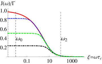
Figure S2: Normalized spectra density function $J(\omega)/\Gamma$ with $\tau_{c}=10$ ns as a function of $\xi$ for selected absorbing boundary, from top to bottom referring to $b=5$ nm, $c=\infty$ (red solid), 50 (blue dotted), 17 (green dashed) and 10 (black dot-dashed) nm. Here we define $\omega_{E}-\omega_{S}=\omega_{0}$ and $\omega_{E}+\omega_{S}=\omega_{2}$.

.1.3 Connection to cooling

Polarization is strongly connected to cooling as in both cases the aim is to prepare the system in a defined state. Thus, as the field of laser cooling is very advanced it is interesting to compare the presented theory with the theory of laser cooling. Cooling is of atoms, ions Chu ; Cohen ; Phillips and mechanical oscillators Igancio ; Florian is divided into two main regimes. The unresolved limit, or Doppler cooling Hansch and the resolved regime or sideband cooling Wineland1 ; Wineland2 ; Stenholm and more advanced methods as dark state cooling Aspect ; Dum ; Giovanna ; Us . In this work we point out for the first time the availability of the regime in which the sideband are resolved for dynamical nuclear polarization.

In both cases the final temperature and the rate are derived from the power spectrum of the noise Cirac_Cooling . For laser cooling the noise originates from the interaction of the atoms with the vacuum while in our case there are two sources of noise. The first one is the noise due to the random feature of the interaction between the NV and the nuclear spins. The second one is the vacuum which induces polarization via the lasers exactly as in the atomic version. In this work we assume that the second one is less significant which means that NV decay time ($T_{1}$) is longer than the decay time induced by the interaction noise.

In our case we have derived directly the rates from the first order term in perturbation theory while for laser cooling the noise and the auxiliary system are being adiabatically eliminated in order to derive a new Master equation for the system alone. The same could be done here. The adiabatic elimination could be done in two stages. In the first stage the noise should be eliminated to derive a Master equation of the nuclear spins and the NV. The adiabatic elimination could be done in the weak coupling limit and assuming Gaussian noise avron ; Spohn ; alicki . At the second stage the NV should be eliminated. In case of no nuclear driving only the the Lindbladian terms and an energy shift survive.

Thus, the final results are readily derived from the power spectrum of the noise (Eq. (S7)), which could also be written as:

$$J(\xi)=\Gamma\frac{81\left(2\xi+5\sqrt{2}\sqrt{\xi}+8\right)}{8\left(4\sqrt{2}\xi^{5/2}+27\sqrt{2}\xi^{3/2}+\xi^{3}+16\xi^{2}+81\xi+81\sqrt{2}\sqrt{\xi}+81\right)}.$$ (S12)

The two interesting limits are derived in $\xi\rightarrow 0,$ which corresponds to the Doppler limit and the limit $\xi\gg 1$ which corresponds to the resolved sideband limit. In the resolved regime, the power spectrum is $\frac{J(\xi)}{\Gamma}=\frac{81}{4\xi^{2}}+O\left(\left(\frac{1}{\xi}\right)^{5/2}\right)$ and thus the final occupation is $1-\frac{81}{2\xi^{2}}+O\left(\left(\frac{1}{\xi}\right)^{5/2}\right),$ which deviates from full polarization with the scaling of $\bigg{(}\frac{1}{\omega_{0}\tau_{c}}\bigg{)}^{2}.$ In comparison to atom or ion cooling in which the occupation behaves as $\bigg{(}\frac{\gamma}{\nu}\Bigg{)}^{2},$ where $\nu$ is the trap frequency which is analogous to $\omega_{0}$ and $\gamma$ is the decay rate which is analogous to the correlation time. The analogy between the correlation time and $\gamma$ is due to the fact that $\gamma$ sets the correlation time in the atomic case. It can be seen that the same scaling is achieved up to the proportionality coefficient.

In the unresolved limit, i.e., the Doppler limit, the power spectrum behaves as $1-\frac{3\sqrt{\xi}}{8\sqrt{2}}+O\left(\xi^{3/2}\right)$ and thus the final occupation is $\frac{3}{4\sqrt{2}}\sqrt{\omega\tau_{c}}.$ Due to the $\sqrt{\xi}$ scaling the effective temperature is not only a function of the decay rate as is in the laser cooling case, but a function of the energy gap as well, meaning, the final temperature is $\sqrt{\frac{\omega}{\tau_{c}}}.$

.1.4 Restricted uniform diffusion with absorbing boundary

Here we isolate the contribution of the polarization transfer from the solvent spins located in the shell $b<R<c$, in which $c$ is the variable radial distance from the center of the nanodiamond. Therefore, assuming absorption boundary condition at the radial distance $c$ from the center of the nanodiamond, we can have

$$J_{l}(\xi)=Re\Big{\{}\frac{2n_{s}}{\xi^{2}D_{T}b}\Big{[}\frac{1-l^{3}}{3}-\frac{3(1+l^{5})}{\xi^{2}}+\frac{1}{C_{2}}(\frac{6l^{3}}{\xi^{4}}-\frac{9C_{1}}{\xi^{3}}-\frac{l^{4}C_{3}}{\xi})\Big{]}\Big{\}},$$ (S13)

in which

$$C_{1} = i_{2}(\xi)k_{2}(\xi/l)-k_{2}(\xi)i_{2}(\xi/l),$$ (S14)

$$C_{2} = i^{\prime}_{2}(\xi)k_{2}(\xi/l)-k^{\prime}_{2}(\xi)i_{2}(\xi/l),$$

$$C_{3} = i^{\prime}_{2}(\xi)k^{\prime}_{2}(\xi/l)-k^{\prime}_{2}(\xi)i^{\prime}_{2}(\xi/l),$$

with $l=b/c$. Here $i_{2}(\xi)$ and $k_{2}(\xi)$ are the related modified spherical Bessel functions HalleS . To elucidate the resulting interplay of the molecular frequency and the spectrometer frequency, suppose $b=5$ nm, we also show the complete normalized frequency spectrum for selected absorbing boundary $c=\infty$, 50, 17 and 10 nm, see Fig. S2. It’s also very important to notice that, in the low frequency limit, the normalized spectra density has substantial contribution from solvent spins far beyond the first hydration layer, which enhances the polarization transfer rate.

.2 Optical nuclear spin polarization with nanodiamonds

.2.1 Random orientations of the NV spins in nanodiamonds

Zero-field and external magnetic field distribution: In the laboratory frame the applied magnetic field defines the z-axis, the NV is placed at the origin of the coordinate system. The Hamiltonian of the electron spin is then Chen2

$$H_{NV} = (\gamma_{e}B+\delta(\theta))S_{z}+D(\theta)S_{z}^{2}$$ (S15)

in which

$$D(\theta)=\frac{D(1+3\cos(2\theta))+3E(1-\cos(2\theta))}{4},\ \ \ \ \delta(\theta)=\frac{\gamma_{e}B|G_{1}|^{2}}{(\gamma_{e}B)^{2}-[D(\theta)]^{2}}+\frac{|G_{2}|^{2}}{2\gamma_{e}B},$$ (S16)

with $G_{1}=\frac{(D-E)\sin\theta\cos\theta}{\sqrt{2}}$, $G_{2}=\frac{D+3E+(E-D)\cos 2\theta}{4}$, zero-field splitting $D=(2\pi)2.87$ GHz and the local strain $E=(2\pi)20$ MHz. Clearly, the random orientations of the NV centers cause a variation of the zero-field splitting $D(\theta)$ across the entire interval $[-(2\pi)1.43\mbox{GHz},(2\pi)2.87\mbox{GHz}]$ and $\delta(\theta)$ across the interval $[0\mbox{MHz},(2\pi)140\mbox{MHz}]$ as shown in Fig. S3a and b, respectively.

Considering the ground state, the states $m_{s}=0$ and $m_{s}=-1$ manifold form a two-level system, a microwave (MW) field of frequency $\omega_{M}$ is applied as a drive of the spin transitions $|-1\rangle\leftrightarrow|0\rangle$, $H_{dri}=\Omega_{M}S_{x}\cos\omega_{M}t$ ($\Omega_{M}$ is the Rabi frequency of the driving field and $\omega_{M}$ is its frequency). Working in a frame that rotates with the microwave frequency $\omega_{M}$, we find

$$H = \frac{\Omega}{2}(|0\rangle\langle-1|+|-1\rangle\langle 0|)+\epsilon(\theta)|-1\rangle\langle-1|+(|-1\rangle\langle-1|)\cdot\mathbf{A}\cdot\vec{I}+\gamma_{n}BI_{z},$$ (S17)

The detuning is given by $\epsilon(\theta)=D(\theta)-\gamma_{e}B-\delta(\theta)+\omega_{M}$, and $\Omega=\Omega_{M}/\sqrt{2}$. Representing the system with the electronic dressed states $|\pm\rangle=\frac{1}{\sqrt{2}}(|-1\rangle\pm|0\rangle)$ and defining the Pauli operator as $\sigma_{z}=\frac{1}{2}(|+\rangle\langle+|-|-\rangle\langle-|)$, $\sigma_{x}=\frac{1}{2}(|+\rangle\langle-|+|-\rangle\langle+|)$, then the polarisation transfer dynamics is described by

$$H_{trans} = \Omega\sigma_{z}+\epsilon\sigma_{x}+\omega_{S}I_{z^{\prime}}+a_{z^{\prime}}\sigma_{z}I_{z^{\prime}}+a_{x^{\prime}}\sigma_{x}I_{x^{\prime}}.$$ (S18)

Here $\omega_{S}=\gamma_{n}\vec{B}-\vec{A}$, And we can rewrite this Hamiltonian as Equation (S4).

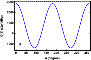
Figure S3: a, Zero-field distribution $D(\theta)$ of the NV spins in nanodiamonds with $D=(2\pi)2.87$ GHz and $E=(2\pi)20$ MHz. b, The second order corrections which induce a energy distribution $\delta(\theta)$. c, The detuning distributions $\Delta^{\prime}=\epsilon-\epsilon_{0}$ vs the angle deviations for $\varepsilon_{0}=\epsilon(90^{\circ})$ presented by the red dashed line and $\epsilon_{0}=\epsilon(0^{\circ})$ by the blue solid line, respectively.

Optical initialization: A randomly oriented nanodiamond ensemble concerns the optical polarisation of electron spins of the NV center. For bulk diamonds, the magnetic field can be aligned with the principal axis of the NV center and the electronic spin of the NV center can be optically polarised to the state $|m_{s}=0\rangle$ by illumination with a $532$ nm green laser. However, although in the laboratory frame of reference a strong magnetic field is applied along the $z$-direction, $\gamma_{e}B_{z}\gg D$, for an ensemble of randomly oriented nanodiamonds, the NV centers will be optically pumped to the state $|m_{s}=0\rangle_{\theta}$ that is defined by the relative orientation of the NV center with respect to the externally applied magnetic field which defines the laboratory frame Chen2 . Here the misalignment angle between the NV-axis and the magnetic field is $\theta$.

As discussed in Ref. Chen2 , we have two coordinate systems which can be transformed into each other and, employing of $S_{z_{\theta}}=\cos\theta S_{z}-\sin\theta(\cos\phi S_{x}-\sin\phi S_{y})$, we can express the eigenstate $|m_{s}=0\rangle_{\theta}$, i.e. in the lab frame,

$$|m_{s}=0\rangle_{\theta}=\cos\theta|0\rangle+\frac{\sin\theta}{\sqrt{2}}(e^{i\phi}|+1\rangle-e^{-i\phi}|-1\rangle).$$ (S19)

If $\theta$ is large, the eigenstate $|0\rangle$ of the NV center in the laboratory frame differs significantly from the zero-field eigenstate $|0\rangle_{\theta}$ of the NV center. Hence optical initialisation of randomly oriented NV centers lead to very different states depending on the orientation of the NV center.

Notice that for small misalignment between the NV center and external magnetic field, the initialisation of the NV center is well approximated to $|0\rangle$. Indeed, for $\theta<10^{\circ}$, we can arrive significant polarisation of the electron spins along the quantisation axis defined by the external magnetic field $P_{NV}\simeq 1$. For $\theta\in[80^{\circ},100^{\circ}]$, the population in state $|0\rangle$ is very small and the initial state is well approximated by $\frac{1}{\sqrt{2}}(e^{i\phi}|+1\rangle-e^{-i\phi}|-1\rangle)$. In the subspace spanned by the states $\{|0\rangle,|-1\rangle\}$, the NV spin is well-polarized in state $|-1\rangle$ with polarization $P_{NV}\simeq 0.5$. So consider a continual optical pumping, it’s reasonable to have the initial polarization of the NV spin $P_{C}\simeq 0.25$.

Detuning from the resonance: MW field is applied to have $\epsilon_{0}=\Omega=(2\pi)8\sqrt{2}$ MHz which matches the resonant condition $\omega_{S}=\omega_{E}=(2\pi)16$ MHz. Since high polarization is achieved for $\theta<10^{\circ}$ and $\theta\in[80^{\circ},100^{\circ}]$, assume two resonant points with $\epsilon_{0}=\epsilon(0^{\circ})$ or $\epsilon_{0}=\epsilon(90^{\circ})$, we calculate the detuning from the resonance which is defined as $\Delta^{\prime}=\epsilon(\theta)-\epsilon_{0}$ and varies with the angle deviation from $0^{\circ}$ and $90^{\circ}$, respectively. As shown in Fig. S3c, if the angle deviation $\Delta\theta\sim 4^{\circ}$, this detuning reaches $(2\pi)20$ MHz both for $\theta<10^{\circ}$ and $\theta\in[80^{\circ},100^{\circ}]$.

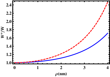
Figure S4: The ratio of polarization transfer with and without eccentricity vs the distance from the center of the nanodiamond. The red dashed and blue solid line show the dependence of comparison of the polarization built up for $\omega_{S}=(2\pi)16$ MHz, $\Delta_{0}=\Omega=(2\pi)8\sqrt{2}$ MHz, and $\Delta^{\prime}=0$ and $\Delta^{\prime}=(2\pi)10$ MHz, respectively.

.2.2 Off-center effect

It’s quite normal when the NV spin is not located in the center of the nanodiamond, so we intend to discuss the polarization transfer under the off-center effect. Suppose a NV center is located off-center and its distance from the center of the nanodiamond is $\rho$. Consider a series expansion in terms of the eccentricity parameters, we can include the off-center effect in the spectra density function which is given by Albrand

$$J^{O}(\xi)=[J(\xi)]\times[(1+\frac{1}{6}\sum_{L=1}^{\infty}(L+1)(L+2)(2L+3)\rho^{2L}\frac{Re[J^{L+2}(\xi)]}{J(\xi)}],$$ (S20)

where

$$J^{L+2}(\xi)=Re[\frac{2n_{s}}{i\xi D_{T}b}\{\frac{1}{2L-1}-\frac{L+1}{i\xi}[1+\frac{(L+1)K_{L+1/2}(\sqrt{i\xi})}{\sqrt{i\xi}K_{L-1/2}(\sqrt{i\xi})}]^{-1}\}],$$ (S21)

with a modified Bessel function $K_{\mu}(\sqrt{i\xi})$. Thus the rate of polarization transfer including off-center effect is given by $W^{O}=W^{O}_{0}-W^{O}_{2}=\alpha_{0}(J^{O}(\omega_{0})-J^{O}(\omega_{2}))$. Fig. S4 illustrates the dependence of the polarization built-up on the eccentricity of the NV center. One can find that polarization built up only is enhanced by factor 1.7 ($\Delta^{\prime}=0$ MHz) or 2.4 ($\Delta^{\prime}=(2\pi)10$ MHz). It is manifested that the polarization transfer is benefited by the eccentricity due to the reduced distance between the NV and the neighboring nuclear spins, but this enhancement is not significant. The possible main reason is the long range nature of the spectral density function, which includes contributions from a large amount of the distant solvent spins.

.2.3 Optical penetration depth

There are two main limitations on the penetration depth when applying optical irradiation to the polarisation structure of the hydrogel containing imobilized diamond: scattering due to nanodiamonds and optical absorption (mainly by NV centre spins). Taking into account the optical cross section of the NV centres and the relatively low NV concentration in this setup we expect the optical penetration depth by the NVs to be a little larger than 1 mm. The optical scattering due to nanodiamonds could become an issue which limits the total penetration depth. As the nanodiamond size is small compared to the optical wavelength, but not negligibly so, we use Mie scattering to calculate the optical transmission through our setup (taking into account only the scattering from the nanodiamonds). It can be seen that the optical penetration decreases sharply with the nanodiamond radius, see Fig. S5. However, for the ND size of interest $b=5$ nm, the scattering from NDs in 1 mm is almost negligible.

Figure S5: The optical transmission through our setup dependence on the nanodiamond radius, taking into account Mie scattering from the nanodiamonds. We assume 1 mm thickness and 12% ND concentration. The black solid and green dashed lines correspond to a refractive index of the medium in between the nanodiamonds of water and air respectively.

References

- (1) F. Bloch, W. W. Hansen, and M. Packard, Phys. Rev. 70, 474 (1946).
- (2) E. M. Purcell, H. C. Torrey, and R. V. Pound, Phys. Rev. 69, 37–38 (1946).
- (3) M. Law et al, Radiology 222, 715 (2002).
- (4) C. Luchinat and G. Parigi, Appl. Magn. Reson. 34, 379 (2008).
- (5) I. Bertini et al Angew. 117, 2263 (2005).
- (6) Y.E. Nesmelov, A. Gopinath, and D.D. Thomas J. Magn. Reson. 167, 138–146 (2004).
- (7) A. Abragam, The principles of nuclear magnetism. Oxford university press, 1961, no. 32.
- (8) E. R. McCarney et al, Proc. Natl. Acad. Sci. 104, 1754 (2007).
- (9) E. R. McCarney and S. Han, J. Magn. Reson. 190, 307 (2008).
- (10) S. Ebert et al, Appl. Magn. Reson. 43, 195 (2012).
- (11) W. Anderson and R. Freeman, J. Chem. Phys. 37, 85 (1962).
- (12) S. Gabl, O. Steinhauser, and H. Weingärtner, Angew. 125, 9412 (2013).
- (13) A. Abragam and M. Goldman, Rep. Prog. Phys. 41, 395 (1978).
- (14) W. T. Wenckebach, Appl. Magn. Reson. 34, 227–235 (2008).
- (15) N. B. Manson, J. P. Harrison, and M. J. Sellars, Phys. Rev. B 74, 104303 (2006).
- (16) F. Jelezko et al, Phys. Rev. Lett. 93, 130501 (2004).
- (17) Q. Chen et al, arXiv preprint arXiv:1504.02368, 2015.
- (18) J.M. Cai, F. Jelezko, M. B. Plenio, and A. Retzker, New J. Phys. 15, 013020 (2013).
- (19) J.-P. King, et al., E-print arXiv:1501.02897., 2015.
- (20) G. A. Álvarez, C. O. Bretschneider, R. Fischer, et al.,E-print arXiv:1412.8635, 2014.
- (21) J.M. Cai et al, New J. Phys. 14, 113023 (2012).
- (22) J.M. Cai, A. Retzker, F. Jelezko, and M. B. Plenio, Nat. Phys. 9, 168 (2013).
- (23) P. London et al, Phys. Rev. Lett. 111, 067601 (2013).
- (24) Supplementary information.
- (25) S. Hartmann and E. Hahn, Phys. Rev. 128, p. 2042 (1962).
- (26) I. Solomon, Phys. Rev. 99, 559 (1955).
- (27) L. P. Hwang and J. H. Freed, J. Chem. Phys. 63, 4017–4025 (1975).
- (28) B. Halle, J. Chem. Phys. 119, 372(2003).
- (29) K. Krynicki, C. D. Green, and D. W. Sawyer, Faraday Discuss. Chem. Soc. 66, 199 (1978).
- (30) Y. E. Shapiro, Prog. Polym. Sci. 36, 1184 (2011).
- (31) H. Huang et al, Nano Lett. 7, 3305 (2007).
- (32) E. von Haartman et al, J. Mat. Chem. B 1, 2358-2366 (2013).
- (33) D. Abrams et al, Nano Lett. 14, 2471 (2014).

References

- (1) I. Solomon, Phys. Rev., 99(2): 559, 1955.
- (2) L. P. Hwang, J H. Freed J. Chem. phys. 1975, 63(9): 4017-4025.
- (3) B. Halle J. Chem. phys. 2003, 119(23): 12372-12385.
- (4) D. Abrams, M. E. Trusheim, D. R. Englund, et al. Nano Lett. vol. 14(5): p. 2471, 2014.
- (5) W. T. Wenckebach, Applied Magnetic Resonance, vol. 34, no. 3-4, pp. 227–235, 2008.
- (6) S. Chu, Rev. Mod. Phys. 70, 685 (1998).
- (7) C. N. Cohen-Tannoudji, Rev. Mod. Phys. 70, 707 (1998).
- (8) W. D. Phillips, Rev. Mod. Phys. 70, 721 (1998).
- (9) I. Wilson-Rae, N. Nooshi, W. Zwerger, and T. J. Kippenberg Phys. Rev. Lett. 99, 093901 (2007).
- (10) F. Marquardt, Joe P. Chen, A. A. Clerk, and S. M. Girvin Phys. Rev. Lett. 99, 093902 (2007).
- (11) T. Hansch and A. Schawlow, Opt. Commun 13, 68 (1975).
- (12) D. Wineland and H. Dehmelt, Bull. Am. Phys. Soc 20, 637 (1975).
- (13) D. J. Wineland, R. E. Drullinger, and F. L. Walls, Phys. Rev. Lett. 40, 1639 (1978).
- (14) S. Stenholm, Rev. Mod. Phys. 58, 699 (1986).
- (15) A. Aspect, E. Arimondo, R. Kaiser, N. Vansteenkiste, and C. Cohen-Tannoudji, Phys. Rev. Lett. 61, 826 (1988).
- (16) R. Dum, P. Marte, T. Pellizzari, and P. Zoller, Phys. Rev. Lett. 73, 2829 (1994).
- (17) G. Morigi, J. Eschner, and C. H. Keitel Phys. Rev. Lett. 85, 4458 (2000).
- (18) J. Cerrillo, A. Retzker, M. B. Plenio, Phys. Rev. Lett. 104, 043003 (2010).
- (19) J. I. Cirac, R. Blatt, P. Zoller and W. D. Phillips, Phys. Rev. A. 46, 2668 (1992).
- (20) J. E. Avron, O. Kenneth, A. Retzker and M. Shalyt, New Journal of Physics 17, 1367 (2015).
- (21) H. Spohn, J.L. Lebowitz. ,in: S.A. Rice (Ed.), Advances in Chemical Physics, Wiley, New York (1978).
- (22) R. Alicki and M. Fannes, 2001 Quantum Dynamical Systems (Oxford: Oxford University Press)
- (23) Q. Chen, I. Schwarz, F. Jelezko, A. Retzker, and M. B. Plenio,(2015) arxiv.org/1504.02368.
- (24) J. P. Albrand, M. C. Taieb, P. Fries, and E. Belorizky, (1981). The Journal of Chemical Physics, 75(5), 2141-2146.