Prey cannibalism alters the dynamics of Holling-Tanner type predator-prey models

Abstract.

Cannibalism, which is the act of killing and at least partial consumption of conspecifics, is ubiquitous in nature. Mathematical models have considered cannibalism in the predator primarily, and show that predator cannibalism in two species ODE models provides a strong stabilizing effect. There is strong ecological evidence that cannibalism exists among prey as well, yet this phenomenon has been much less investigated. In the current manuscript, we investigate both the ODE and spatially explicit forms of a Holling-Tanner model, with ratio dependent functional response. We show that cannibalism in the predator provides a stabilizing influence as expected. However, when cannibalism in the prey is considered, we show that it cannot stabilise the unstable interior equilibrium in the ODE case, but can destabilise the stable interior equilibrium. In the spatially explicit case, we show that in certain parameter regime, prey cannibalism can lead to pattern forming Turing dynamics, which is an impossibility without it. Lastly we consider a stochastic prey cannibalism rate, and find that it can alter both spatial patterns, as well as limit cycle dynamics.

Aladeen Basheer, Emmanuel Quansah, Schuman Bhowmick and Rana D. Parshad

Department of Mathematics,

Clarkson University,

Potsdam, New York 13699, USA.

1. Introduction

Cannibalism is the act of killing and at least partial consumption of conspecifics. This has been documented in human populations all around the world. It is/has been practiced in various indigenous South American and New Guinean tribes as a social norm [16], and also reported in Africa [23]. It is also practiced among “Aghoris” or witch doctors in Northern India, in the hope of gaining immortality [25]. However, if one steps away from these seemingly macabre and ghoulish human practices, and observes real predator-prey systems, then cannibalism is actually commonplace [8]. It is seen to actively occur in more than 1300 species in nature [24]. Apart from being a fascinating socio-anthropological/ecological subject in its own right, cannibalism can lead to various “counter intuitive” effects as concerns population dynamics. These include the life boat mechanism, where the act of cannibalism causes persistence, in a population doomed to go extinct [12]. It can also induces stability, in an otherwise cycling population [17].

A detailed survey of the current and past mathematical literature on cannibalism, shows that various types of predator-prey models, with the inclusion of cannibalism, have been investigated. These include two species ODE models, three species ODE models incorporating stage structure, two species PDE models, discrete models and integro-differential equation models, as well as recent models of cannibalism that include diseased predators [17, 4, 3, 5, 12].

The two species unstructured ODE models that have been investigated, are of the general type

(1) $$\frac{du}{dt}=u\left(1-\frac{u}{K}\right)-f(u)v,$$

(2) $$\frac{dv}{dt}=-dv+\epsilon f(u)v-cC(u,v),$$

where $u$ is the prey, and $v$ the predator. Here $cC(u,v)$ models cannibalism in the predator, with $c$ being the rate of cannibalism. In such models, cannibalism is seen to have a strong stabilising influence. Kohlmeir [17] was the first to show this, by considering cannibalism in the predator, in the classic Rosenzweig-McArthur model. That is when $f(u)$ is of Holling type II. They showed that predator cannibalism can surprisingly stabilise the unstable interior equilibrium of the model.

We note that cannibalism, has been primarily modeled as an act in the predator species only [10, 34, 17]. Note, there is strong evidence in ecology that cannibalism often occurs in the prey species [27, 26]. Recent experiments with prey cannibalism, show that they can have a significant impact on the population dynamics of predator-prey systems [28]. However, there is not a single model in the mathematical literature, that considers the effect of prey cannibalism in two species unstructured ODE or unstructured PDE models. To the best of our knowledge there are very few works overall, that have considered prey canibalism, in some form or the other. Solis et al. considered the effect of prey cannibalism in a multi component structured model, via integer differential equations [31]. Chow and Jang investigated a structured discrete model with prey cannibalism finding that it may either stabilize or destabilize, depending on cannibalism rates and various other parameters [7]. Also, Zhang et al. considered a three species structured ODE model, with structure and cannibalism in the prey. They showed that cannibalism strengthens the conditions of both global asymptotical stability, and persistence of the interior equilibrium point [37].

Many models of cannibalism with size and stage structure effects have been investigated. The approach in the literature has been to structure the predator class into adults and juveniles and allow predation of the juvenile predator by the adult predator. This essentially yields a three species ODE model. The reader is referred to [5, 4, 37], and again therein cannibalism is seen to provide a stabilising influence, depending on parameter regime. However, depending on model structure and parameter regimes, cannibalism is also seen to destabilize [8] in some cases. Various other classes of models such as integro-differential equation models, as well as discrete models have also been investigated [7, 31, 12].

Since species disperse in space in search of food, shelter, mates and to avoid predators, spatially dispersing populations are often modeled via partial differential equations (PDE)/spatially explicit models of interacting species [36, 21, 22, 29]. Of particular interest to many is the phenomenon of Turing instability, first introduced by Alan Turing [35], which shows that diffusion in a system can lead to pattern forming instabilities. In the context of cannibalism, there are very few works in the literature that deal with spatially explicit models and/or Turing instability. Sun [34] was the first to show that cannibalism in the classical diffusive Rosenzweig-McArthur model, can bring about Turing patterns. This is an impossibility in the system without cannibalism. Fasani et al. [10] considered the same model, but with a general form for the cannibalism term (of which the model of Sun et al. is a special case), and also found that cannibalism can bring about Turing patterns. The other direction does not seemed to have been studied. That is when and under what conditions, can cannibalism remove Turing instability? In the current manuscript we argue that these above approaches, do not capture the full breadth of cannibalism as it exists in nature. We cite the following reasons:

Many mathematical models of predator-prey systems, do not have a symmetric functional responses between predator and prey. For example, the models of Leslie-Gower type [18], and Holling-Tanner type [14]. These models are ubiquitous in the mathematical literature (see [2, 14] and the references therein), however, the effect of cannibalism, in particular the effect of prey cannibalism in such models, has not been considered.

Also, In all of the investigations in the literature, only a deterministic rate of cannibalism, $c$, has been considered. However, predator and prey species are often subject to uncertainties in the environment, modeled best via environmental noise. For these reasons it is possible that the various rates, (birth rate, death rate, predation rate etc.), one considers for modeling purposes, may not be known precisely, and may always involve uncertainty. Yet there are no studies where a model with a “noisy” cannibalism rate has been considered, that is when $c\approx c+``noise"$.

In the current manuscript we consider a Holling-Tanner predator-prey model, with a ratio dependent functional response [1], that has been well studied in the literature [2]. Next we introduce into this model
(a) cannibalism occurring only in the predator species,
(b) cannibalism occuring only in the prey species.
We investigate in detail:
(1) ODE versions modeling (a) and (b).
(2) The PDE, stochastic ODE and stochastic PDE versions modeling (b).


Our contributions therein are the following:
1) We show that predator cannibalism, in certain parameter regime, can indeed stabilize the unstable interior equilibrium, in the ODE case, as expected from the known results on other models, with cannibalism in the predator.
2) We show that prey cannibalism cannot stabilize the unstable interior equilibrium, in the ODE case. This is contrary to what is known about models with cannibalism in the predator.
3) We show that prey cannibalism can destabilize the spatially homogenous equilibrium in the PDE case. In particular, we show that in certain parameter regime such that there is no Turing instability in the Holling-Tanner model, introducing prey cannibalism can actually bring about Turing instability. Alternatively, we show that in certain parameter regime, introducing predator cannibalism cannot bring about Turing instability.
4) We show that in certain parameter regime, if Turing instability does not exist in the model with prey cannibalism, then removing prey cannibalism cannot induce Turing instability.
5) The ODE version of the Holling-Tanner model we consider is known to possess a unique limit cycle. We investigate the effects of a stochastic prey cannibalism rate $c$, on the limit cycle dynamics, finding that classical white noise cannot induce stability.
6) We also consider the effects of a stochastic prey cannibalism rate $c$, on the spatial dynamics, finding that space-time white noise, can significantly alter the spatial dynamics of the model.

2. The model formulation

2.1. The Holling-Tanner model

We first present the following Holling-Tanner model, with ratio dependent functional response in prey, [2].

(3) $$\left.\begin{array}[]{c}\frac{du}{dt}=u\left(1-u\right)-\dfrac{uv}{u+\alpha v}\\ \frac{dv}{dt}=\delta v\left(\beta-\dfrac{v}{u}\right)\end{array}\right\}nc-model$$

We will refer to the above model as the nc-model (no cannibalism) henceforth, and recap certain dynamical aspects of the model. Note, (3) is a nondimensionalised version of the model presented in [2]. The reader is referred to [2], for a complete derivation on the parameters, their biological significance and the non-dimensionalization process. Here $u$ and $v$ are the populations of the prey and predator species respectively. The dynamics of the prey species follows a ratio dependent functional response [1]. The predator is modeled according to the Leslie-Gower scheme [18]. This assumes that the carrying capacity of the predator, is not constant but rather proportional to its food, the prey $u$. Hence a reasonable choice for the carrying capacity $K=K(u)$ is $K(u)=u+d_{3}$. If $d_{3}>0$, the predator is thought of as a generalist, that is it can change its food source in the absence of its favorite prey. If $d_{3}=0$, the predator is thought of as a specialist. In this case the resulting model is of Holling-Tanner type [14]. Here $\beta$ is the intrinsic growth rate of the predator $v$, and $\alpha$ is essentially given by $\alpha=\frac{\mbox{prey \ handling \ time}}{\mbox{ prey \ capture \ rate }}$.

The non-trivial steady state $\left(u_{nc},v_{nc}\right)$ is given by:

$$u_{nc}=1-\dfrac{\beta}{1+\alpha\beta},\text{ \ \ }v_{nc}=\beta\left(1-\dfrac{\beta}{1+\alpha\beta}\right)$$

since we require

$$u_{nc}>0,\ \Longrightarrow\ 1>\dfrac{\beta}{1+\alpha\beta}\$$

Thus we obtain the following restriction on $\beta$ due to a feasibility requirement,

$$\beta<\dfrac{1}{1-\alpha}$$

For stability we require that the $Trace$ $J^{nc}<0$ which implies

$$\dfrac{\beta}{\alpha\beta+1}+\dfrac{\beta}{\left(\alpha\beta+1\right)^{2}}-1<\beta\delta$$

As the determinant $Det$ $J^{nc}>0$, is always positive, as we have $\Rightarrow\beta<\dfrac{1}{1-\alpha}$, which is always true as this is a feasibility condition.

2.2. The Holling-Tanner model with predator cannibalism

We now consider the inclusion of predator cannibalism in (3). This yields the following model

(4) $$\left.\begin{array}[]{c}\dfrac{du}{dt}=u\left(1-u\right)-\dfrac{uv}{u+\alpha v}\\ \dfrac{dv}{dt}=\delta v\left(\beta_{1}-\dfrac{v}{\gamma u+cv}\right)\end{array}\right\}predator\ cannibalism\ model$$

In deriving the above model we make the following assumptions

• The predator $v$ is depredating on the prey species $u$, as well as on its own species $v$.

• Hence the food source of $v$ is $\gamma u+cv$, where $cv$ is the cannibalism term, with cannibalism rate $c$. Here we assume $c+\gamma\approx 1$, with $\gamma<1,c<1$. Thus the food intake of the predator stays roughly the same, even if it turns into a cannibal. It starts eating less prey $u$, so $\gamma<1$, and now also eats some conspecifics, so $0<c<1$.

• There is a clear gain of energy to the cannibalistic predator, from the act of cannibalism. This gain results in an increase in reproduction in the predator. This in turn leads to a gain in predator population, modeled via adding a $\beta_{1}v$ term to the predator equation. We therefore assume $\beta_{1}>\beta$.

The non-trivial steady state $\left(u_{c},v_{c}\right)$ is given by

(5) $$u_{c}=\left(1-\dfrac{\beta_{1}\gamma}{\alpha\beta_{1}\gamma-c\beta_{1}+1}\right),\\ v_{c}=\left(\dfrac{\gamma\beta_{1}}{1-\beta_{1}c}\right)u_{c}$$

since $u_{c}>0$ we obtain

$\left(1-\dfrac{\beta_{1}\gamma}{\alpha\beta_{1}\gamma-c\beta_{1}+1}\right)>0$ and due to the assumptions and feasibility conditions, $\gamma<1,\\ 1-\beta_{1}c>0$ we have

$\alpha\gamma-\gamma+\dfrac{1}{\beta_{1}}\ >c$

The Jacobian Matrix at $(u_{c},v_{c})$:

$J^{c}=\left(\begin{array}[]{ccc}\allowbreak-u_{c}+\dfrac{\left(1-\beta_{1}c+\alpha\gamma\beta_{1}\right)^{2}}{\gamma\beta_{1}\left(1-\beta_{1}c\right)}&&\allowbreak-\dfrac{\left(c\beta_{1}-1\right)^{2}}{\left(\alpha\beta_{1}\gamma-c\beta_{1}+1\right)^{2}}\\ &&\\ \allowbreak\beta_{1}^{2}\gamma\delta&&\allowbreak\beta_{1}\delta\left(c\beta_{1}-1\right)\end{array}\right)$

Notice that $J_{12}$ and $J_{22}$ are negative since $\gamma<1$ and $1-\beta_{1}c>0$.

Det $J^{c}$=$\left(-u_{c}+\dfrac{\left(1-\beta_{1}c+\alpha\gamma\beta_{1}\right)^{2}}{\gamma\beta_{1}\left(1-\beta_{1}c\right)}\right)\allowbreak\left(\beta_{1}\delta\left(c\beta_{1}-1\right)\right)+\left(\dfrac{\allowbreak\beta_{1}^{2}\gamma\delta\left(c\beta_{1}-1\right)^{2}}{\left(\alpha\beta_{1}\gamma-c\beta_{1}+1\right)^{2}}\right)>0$

$T_{c}=-u_{c}+\dfrac{\left(1-\beta_{1}c+\alpha\gamma\beta_{1}\right)^{2}}{\gamma\beta_{1}\left(1-\beta_{1}c\right)}+\allowbreak\beta_{1}\delta\left(c\beta-1\right)$

We can thus state the following lemma

Lemma 2.1.

Consider a parameter set s.t. $T_{nc}>0$, that is the interior equilibrium point $\left(u_{nc},v_{nc}\right)$ of the no cannibalism model (3) is unstable. If $\gamma<\dfrac{\beta}{\beta_{1}}$ then there exists a cannibalism rate $c$ s.t $T_{c}<0$. This implies that the unstable interior equilibrium point $\left(u_{nc},v_{nc}\right)$ of the no cannibalism model (3) can be stabilised via predator cannibalism. However If $\gamma>\dfrac{\beta}{\beta_{1}}$ then the unstable interior equilibrium point $\left(u_{nc},v_{nc}\right)$ of the no cannibalism model (3) cannot be stabilised via predator cannibalism.

Proof.

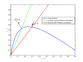
We take a simple geometric approach and visualise the nullclines below in fig. 1. In order to shift the nullcline to the right due to predator cannibalism, we will require that the slope of the predator nullcline is less than $\beta$. That is $\dfrac{\gamma\beta_{1}}{1-\beta_{1}c}<\beta$. If $\dfrac{\gamma\beta_{1}}{\beta}=1-\epsilon<1$, we can always choose $c$ small enough s.t $1-\epsilon<1-\beta_{1}c$. In this case the slope of the predator nullcline with predator cannibalism will be less than $\beta$. If on the other hand $\dfrac{\gamma\beta_{1}}{\beta}<1$, this is clearly an impossibility as $\dfrac{\gamma\beta_{1}}{\beta}>1>1-\beta_{1}c$.

Figure 1. Here we see the nullclines of the model (3) vs the nullclines of model (4). We see that if $\gamma<\dfrac{\beta}{\beta_{1}}$ predator cannibalism, decreases the slope of the predator nullcline, shifting it to the right, and making it possible for $J^{c}_{11}<0$ and hence for $T_{c}<0$, while $T_{nc}>0$. In this figure the parameters chosen are $\alpha=0.89,\beta=3.5,c=0.18,\delta=0.01,\gamma=0.2$.

∎

Remark 1.

The cannibals feeding rate of prey $\gamma$ and the ratio $\dfrac{\beta}{\beta_{1}}$, are critical in terms of stability. The stability condition tells us that if the cannibal eats less prey so $\gamma$ is small in comparison to $\dfrac{\beta}{\beta_{1}}$, then only a little bit of feeding of conspecifics is enough to stabilize the dynamics.

2.3. The Holling-Tanner model with prey cannibalism

We now consider the inclusion of prey cannibalism in (3). This yields the following model

(6) $$\left.\begin{array}[]{c}\dfrac{du}{dt}=u\left(1+c_{1}-u\right)-\dfrac{uv}{u+\alpha v}-c\dfrac{u^{2}}{u+d}\\ \dfrac{dv}{dt}=\delta v\left(\beta-\dfrac{v}{u}\right)\end{array}\right\}prey\ cannibalism\ model$$

In deriving the above model we make the following assumptions

• The prey $u$ is depredating on its own species $u$.

• Here the generic cannibalism term $C(u)$, is added in the prey equation, and is given by

  $$C(u)=c\times u\times\dfrac{u}{u+d}.$$

  That is the functional response of the cannibalistic prey is of Holling type II, with cannibalism rate $c$.

• There is a clear gain of energy to the cannibalistic prey, from the act of cannibalism. This gain results in an increase in reproduction in the prey. This in turn leads to a gain in prey population, modeled via adding a $c_{1}u$ term to the prey equation.

• We restrict $c_{1}<c$, as it takes depredation of a number of prey by the cannibal to produce one new offspring.

The non-trivial steady state $\left(u_{c},v_{c}\right)$ is given by

$$u_{c}=\dfrac{-\left(m+d+c-c_{1}-1\right)+\sqrt{\left(m+d+c-c_{1}-1\right)^{2}+4d(1-m)+4dc_{1}}}{2}$$

where $m=\dfrac{\beta}{\alpha\beta+1}<1$.

The feasibility conditions are divided into the following cases,

1. if $m<1+c_{1}$ and $m+d+c\geq 1+c_{1}$

2. if $m<1+c_{1}$ and $m+d+c<1+c_{1}$

The Jacobian matrix of system (6) at the point $\left(u_{c},v_{c}\right)$ given by:

$J^{c}=\allowbreak\left(\begin{array}[]{ccc}\left(\dfrac{\beta}{\left(1+\alpha\beta\right)^{2}}-u_{c}-\dfrac{cdu_{c}}{\left(u_{c}+d\right)^{2}}\right)&&-\dfrac{1}{\left(1+\alpha\beta\right)^{2}}\\ &&\\ \beta^{2}\delta&&-\beta\delta\end{array}\right)$

The conditions for stability are:

$$\mbox{Trace}\ J^{c}<0,\mbox{det}\ J^{c}>0\$$

The Trace $J^{c}<0$ if

$$\left(\dfrac{\beta}{\left(1+\alpha\beta\right)^{2}}-u_{c}-\dfrac{cdu_{c}}{\left(u_{c}+d\right)^{2}}\right)<\beta\delta$$

The above implies

$$\left(\dfrac{\beta}{\left(1+\alpha\beta\right)^{2}}-u_{c}-\beta\delta\right)\dfrac{\left(u_{c}+d\right)^{2}}{du_{c}}<c$$

Note

$$\mbox{Det}\ J^{c}=\dfrac{\beta\delta u_{c}[d^{2}+2du_{c}+cd+(u_{c})^{2}]}{d^{2}+2du_{c}+(u_{c})^{2}}>0$$

This is always true.

2.4. Effect of prey cannibalism on stability

We now ask the following question. Consider the nc-model in a parameter regime, such that the interior equilibrium $(u_{nc},v_{nc})$ is stable. Can prey cannibalism destabilize this equilibrium? If so, under what conditions? This is settled via the following lemma,

Lemma 2.2.

For any selection of parameters, there always exists a cannibalism rate $c$  s.t the interior equilibrium point $\left(u_{nc},v_{nc}\right)$ of the $nc$-model is stable, while the interior equilibrium point $\left(u_{c},v_{c}\right)$ of the prey cannibalism model is unstable.

Proof.

Note that the condition under which the interior equilibrium point $\left(u_{nc},v_{nc}\right)$ of the $nc$-model is stable, while the interior equilibrium point $\left(u_{c},v_{c}\right)$ of the prey cannibalism model is unstable, is

$$\left(T_{nc}<0<T_{c}\right)$$

The above is equivalent to showing that $\exists c$  s.t

$$u_{c}+\dfrac{cdu_{c}}{\left(u_{c}+d\right)^{2}}<u_{nc}.$$

Note

$$u_{c}+\dfrac{cdu_{c}}{\left(u_{c}+d\right)^{2}}<u_{c}+\dfrac{c\frac{\left(u_{c}+d\right)^{2}}{2}}{\left(u_{c}+d\right)^{2}}=u_{c}+\dfrac{c}{2}<u_{nc}.$$

Thus we want to show

$$u_{c}+\dfrac{c}{2}<u_{nc}.$$

Now $u_{c}=\dfrac{-\left(m+d+c-c_{1}-1\right)+\sqrt{\left(m+d+c-c_{1}-1\right)^{2}+4d(1-m)+4dc_{1}}}{2}$

It is easily computable that

$$\dfrac{d\left(u_{c}\right)}{dc}=-\dfrac{1}{2}+\dfrac{\left(m+d+c-1-c_{1}\right)}{2\sqrt{\left(m+d+c-1-c_{1}\right)^{2}+4d(1-m)+4dc_{1}}}<0,$$

that is $u_{c}$ is monotonically decreasing in $c$, and so decreasing $c$ to a small enough level, will eventually cause $u_{c}+\dfrac{c}{2}<u_{nc}$. This proves the lemma. ∎

We next ask the following question. Consider the nc-model in a parameter regime, such that the interior equilibrium $(u_{nc},v_{nc})$ is unstable. Can prey cannibalism stabilize this equilibrium? If so, under what conditions? In order to answer this question, we must further analyse the dynamical behavior of the prey cannibalism model. We state our result via the following lemma:

Lemma 2.3.

If  $\left(m+d+c\right)<1+c_{1}$ then then there does not exist a cannibalism rate $c$  s.t $u_{c}+\dfrac{cdu_{c}}{\left(u_{c}+d\right)^{2}}>u_{nc}$. This implies that no amount of prey cannibalism can stabilize the unstable interior equilibrium point $\left(u_{nc},v_{nc}\right)$ of the prey cannibalism model.

Proof.

The explicit condition under which the equilibrium point $\left(u_{nc},v_{nc}\right)$ of the nc-model is unstable and the equilibrium point $\left(u_{c},v_{c}\right)$ of the prey cannibalism model is stable is given by

$$\left(T_{c}<0<T_{nc}\right)$$

This is equivalent to $u_{c}+\dfrac{cdu_{c}}{\left(u_{c}+d\right)^{2}}<u_{nc}$. Now,

$$u_{c}+\dfrac{cdu_{c}}{\left(u_{c}+d\right)^{2}}=u_{c}+\dfrac{c}{2}\dfrac{2du_{c}}{\left(u_{c}+d\right)^{2}}<u_{c}+\dfrac{c}{2}\dfrac{\left(u_{c}+d\right)^{2}}{\left(u_{c}+d\right)^{2}}=u_{c}+\dfrac{c}{2}.$$

Thus if we can show

$u_{c}+\dfrac{c}{2}<u_{nc}$

then this will imply that $u_{c}+\dfrac{cdu_{c}}{\left(u_{c}+d\right)^{2}}<u_{c}+\dfrac{c}{2}<u_{nc}$.

We let $f(c)=u_{c}+\dfrac{c}{2}-u_{nc}$, note $f(0)=0$.

We next compute the derivative of $f$ w.r.t. $c$.

$$f(c)$$

$$=\dfrac{-\left(m+d+c-1-c_{1}\right)+\sqrt{\left(m+d+c-1-c_{1}\right)^{2}+4d(1-m)+4dc_{1}}}{2}+\dfrac{c}{2}-u_{nc}$$

$$\Rightarrow f^{{}^{\prime}}(c)=-\dfrac{1}{2}+\dfrac{\left(m+d+c-1-c_{1}\right)}{2\sqrt{\left(m+d+c-1-c_{1}\right)^{2}+4d(1-m)+4dc_{1}}}+\dfrac{1}{2}$$

$$=\dfrac{\left(m+d+c-1-c_{1}\right)}{2\sqrt{\left(m+d+c-1-c_{1}\right)^{2}+4d(1-m)+4dc_{1}}}$$

$$<0$$

since $\left(m+d+c\right)<1+c_{1}$. This implies that $f^{{}^{\prime}}(c)<0$. Thus $f(c)$ is decreasing, and since $f(0)=0$, it must be that $f(c)=u_{c}+\dfrac{c}{2}-u_{nc}<0$, for all $c$. Thus $u_{c}+\dfrac{cdu_{c}}{\left(u_{c}+d\right)^{2}}<u_{c}+\dfrac{c}{2}<u_{nc}$. This proves the lemma. ∎

Remark 2.

The above proof is under the first feasibility condition $\left(m+d+c\right)<1+c_{1}$, that is small cannibalism parameter $c$. Numerically, we could not find a cannibalism rate $c$ such that the equilibrium point $\left(u_{nc},v_{nc}\right)$ of the nc-model is unstable while the equilibrium point $\left(u_{c},v_{c}\right)$ of the prey cannibalism model is stable, under the second feasibility condition $\left(m+d+c\right)>1+c_{1}$, that is when the cannibalism parameter $c$ can be very large. We tried a parameter sweep of all parameters in the interval $[0,10]$. We thus beleive that prey cannibalism cannot stabilise, whatever the range of the cannibalism parameter $c$ be, large or small. However, the large $c$ case is unproven at this point.

Nonetheless, we make the following conjecture

Conjecture 1.

There does not exist a cannibalism rate $c$, such that the equilibrium point $\left(u_{nc},v_{nc}\right)$ of the nc-model is unstable while the equilibrium point $\left(u_{c},v_{c}\right)$ of the prey cannibalism model is stable.

3. The effect of Noisy cannibalism rate on limit cycle dynamics

In this section we aim to investigate the effect of a noisy cannibalistic parameter on the limit cycle dynamics in the prey cannibalism model. We proceed by stating the following lemma,

Lemma 3.1.

The solutions of system (6) are always positive and bounded, furthermore there exists $T\geq 0$ such that $0<u(t)<1+c_{1},$ $0<v(t)<\beta(1+c_{1}),$ for all $t>T$.

Proof.

The positivity easily follows by the quasi monotonicity of the reaction terms. For boundedness note that for system (6), we have

$\frac{du}{dt}\leq u(1+c_{1}-u)$

A standard comparison argument shows that $\lim_{t\rightarrow\infty}u(t)\leq 1+c_{1}.$It follows that there exists $T>0$ such that $u(t)<1+c_{1},$ for $t>T$.

From the second equation of system (6), we see that, for $t>T$,

A standard comparison argument shows that $\lim_{t\rightarrow\infty}v(t)\leq(1+c_{1})\beta$. ∎

Now, it can be shown that under certain parametric restrictions, there exists a limit cycle in the prey cannibalism model (6). We state this via the following lemma,

Lemma 3.2.

Consider the prey cannibalism model (6). Assume that the following conditions hold

(8) $$\alpha\beta+1>\beta,\ \left(\dfrac{\beta}{\left(1+\alpha\beta\right)^{2}}-u_{c}-\beta\delta\right)\dfrac{\left(u_{c}+d\right)^{2}}{du_{c}}>c,$$

then the system possesses at least one limit cycle.

Here $u_{c}$ is the prey equilibrium in model (6).

Proof.

From the local stability analysis, we have that if the above conditions hold, then the positive equilibrium $E_{c}=\left(u_{c},v_{c}\right)$ of system (6) is an unstable node or focus. The existence of a limit cycle now follows from lemma 3.1 and Poincairé-Bendixson theorem [32]. ∎

Remark 3.

Although the existence of a unique limit cycle for the nc-model is well known, and the existence of a limit cycle with the addition of prey cannibalism is seen via lemma 3.2, we are unable to prove uniqueness, in this case. We turn our attention to investigating the effect that a stochastic cannibalism rate has on the limit cycle dynamics.

Biological species are always subject to random environmental fluctuations, be it via climatic factors, or ecological. Also, many times the parameters we use for modeling such processes many not be known with certainty. In this present paper, we only assume that the cannibalism rate $c$ is affected by environmental fluctuations, which is define as mortality rate due to cannibalism. We introduce a stochastic factor in time ${\mathrm{\eta}(t)}$, into the cannibalism rate $(c)$, and so the parameter $c$ is treated as a Gaussian random variable with mean $\hat{c}$ and intensity $\alpha_{1}$. Here ${\mathrm{\eta}(t)}=``\frac{d}{dt}W_{t}"$ is a classical white noise.

(9) $$c\approx\hat{c}+\alpha_{1}{\mathrm{\eta}(t)}.$$

Under these assumptions we consider the following SDE model, where for1simplicity, we redefine mean $\hat{c}$ to be the parameter $c$.

$$du=\left(u\left(1+c_{1}-u\right)-\dfrac{uv}{u+\alpha v}-c\dfrac{u^{2}}{u+d}\right)dt+\alpha_{1}\dfrac{u^{2}}{u+d}dW_{t}$$

$$dv=\delta v\left(\beta-\dfrac{v}{u}\right)dt$$

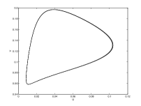
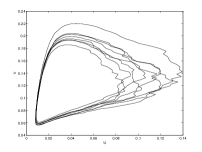
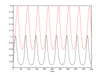
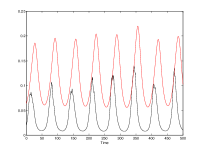
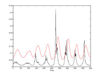
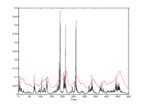
We observe that as $\alpha_{1}$ is increased, the limit cycle dynamics becomes aperiodic, but some cyclicity remains. The noise is unable to stabilise, that is drive the population cycle to a steady state. This is shown via the following plots,

Figure 2. Here we see a limit cycle in nc-model in the left panel (with $\alpha_{1}=0.0$). We observe that the effect of a noisy prey cannibalism rate is to distort the limit cycle, but some cyclicity remains (with $\alpha_{1}=0.1$). For the list of parameters chosen please refer to Table 1.

Figure 3. The left panel in the above is the time series corresponding to the phase plot in the left panel in fig. 2 (with $\alpha_{1}=0.0$). The right panel corresponds to a slightly greater noise intensity (with $\alpha_{1}=0.1$). For the list of parameters chosen please refer to Table 1.

Figure 4. These figures show the effect of further increasing the noise intensity, on the limit cycle dynamics (where the left panel shows $\alpha_{1}=0.5$ and right panel shows $\alpha_{1}=2.0$). For the list of parameters chosen please refer to Table 1.

Remark 4.

Thus it seems that even with some stochasticity in the cannibalism parameter, prey cannibalism is unable to stabilise dynamics. It is well known that large enough noise intensity will drive everything to extinction, but this is an uninteresting case.

This leads us to make the following conjecture

Conjecture 2.

There does not exist a stochastic cannibalism rate $c$, such that the non trivial equilibrium point $\left(u_{nc},v_{nc}\right)$ of the nc-model is unstable, while the nontrivial equilibrium point $\left(u_{c},v_{c}\right)$ of the stochastic prey cannibalism model is stable.

4. The effect of prey cannibalism on Turing instability

Turing instability occurs when the positive interior equilibrium point for an ODE system is stable in the absence of diffusion, but becomes unstable due to the addition of diffusion, that is in the PDE model. This phenomena is also referred to as diffusion driven instability, [35]. To formulate the spatially explicit form of the earlier described ODE models, we assume that the predator and prey populations move actively in space. Random movement of animals occurs because of various requirements and necessities like, search for better food, better opportunity for social interactions such as finding mates [22]. Food availability and living conditions demand that these animals migrate to other spatial locations. In the proposed model, we have included diffusion assuming that the animal movements are uniformly distributed in all directions. The models with diffusion are described as follows

(11) $$\left.\begin{array}[]{c}u_{t}=D_{u}u_{xx}+u(1-u)-{\frac{uv}{u+\alpha v}},\\ v_{t}=D_{v}v_{xx}+\delta v\left(\beta-\frac{v}{u}\right)\end{array}\right\}\ no\ cannibalism\ model$$

and the diffusive model with prey cannibalism

(12) $$\left.\begin{array}[]{c}u_{t}=D_{u}u_{xx}+(1+c_{1})u(1-u)-{\frac{uv}{u+\alpha v}}-\frac{cu^{2}}{u+d},\\ v_{t}=D_{v}v_{xx}+\delta v\left(\beta-\frac{v}{u}\right)\end{array}\right\}\ prey\ cannibalism\ model$$

The spatial domain for the above is $\Omega\subset\mathbb{R}^{1}$. $\Omega$ is assumed bounded, and we prescribe Neumann boundary conditions $u_{x}=v_{x}=0$, for $x\in\partial\Omega$, and suitable initial conditions. The main reason for choosing such boundary conditions is that we are interested in the self-organization of patterns, and zero-flux boundary conditions imply that no external input is imposed [22, 21]. In the numerical simulations we take $\Omega=[0,\pi]$. Here $u(x,t)$ is the density of the prey species at any given time $t$, that is logistically controlled, and predated on by a predator species with density $v(x,t)$.

Remark 5.

For various models, that fall into the above general category, it has been shown that Turing instability exists. However, this is only for certain parameters that lie in the so called Turing space. For parameters outside of that space Turing patterns are an impossibility.

4.1. General criterion for no Turing instability in nc-model

Our goal in the current section is to investigate the conditions under which there is no Turing instability in (11), but there are Turing patterns in (12). Thus we aim to quantify the conditions under which cannibalism in the prey species, can induce Turing patterns.

We begin by linearizing model system (11) about its homogenous steady state $(u_{nc},v_{nc})$, by introducing both space and time-dependent fluctuations. In order to derive the precise conditions for Turing instability there is a well known procedure. We refer the reader to [36]. The calculations therein can be stated via the following theorem,

Theorem 4.1 (Turing Instability Condition).

Consider $(u_{nc},v_{nc})$ which is a spatially homogenous equilibrium point of the model system (11). For a given set of parameters, if at $(u_{nc},v_{nc})$ , the Jacobian $\mathbf{J}=\begin{bmatrix}J_{11}&J_{12}\\ J_{21}&J_{22}\end{bmatrix}$, of the reaction terms, and the diffusion coefficients $D_{u},D_{v}$ satisfy

$$J_{11}+J_{22}<0$$

$$J_{11}J_{22}-J_{21}J_{12}>0,$$

$$D_{v}J_{11}+D_{u}J_{22}>0.$$

$${(D_{v}J_{11}+D_{u}J_{22})^{2}}-4D_{u}D_{v}(J_{11}J_{22}-J_{21}J_{12})>0,$$

then $(u_{nc},v_{nc})$ is said to be linearly stable in the absence of diffusion and linearly unstable in the presence of diffusion.

And easy corollary derived from the above imposes an additional necessary condition for Turing instability

Corollary 1 (Necessary condition for Turing Instability).

If $(u_{nc},v_{nc})$ is a spatially homogenous equilibrium point of the model system (11) which is linearly stable in the absence of diffusion, and linearly unstable in the presence of diffusion, then either $J_{11}<0,J_{22}>0$ or $J_{11}>0,J_{22}<0$, where $\mathbf{J}=\begin{bmatrix}J_{11}&J_{12}\\ J_{21}&J_{22}\end{bmatrix}$, is the Jacobian matrix of the reaction terms.

We begin by focusing on (11), investigated in detail by Banerjee [2]. The results therein reveal that turing instability in model (11) occurs, if $\alpha<1$, for a range of parameters in the so called Turing space.

Note that the jacobin matrix of the reaction terms of (11) at the point $\left(u_{nc},v_{nc}\right)$ is given by

$J=$ $\allowbreak\allowbreak\left(\begin{array}[]{ccc}\dfrac{\beta}{\alpha\beta+1}+\dfrac{\beta}{\left(\alpha\beta+1\right)^{2}}-1&&-\dfrac{1}{\left(\alpha\beta+1\right)^{2}}\\ &&\\ \beta^{2}\delta&&-\beta\delta\end{array}\right)$

Since the parameters $\beta>0,\delta>0$, we always have that $J_{22}<0$. Thus an application of corollary 1 yields the following lemma:

Lemma 4.2.

The equilibrium point $\left(u_{nc},v_{nc}\right)$ cannot be driven unstable via diffusion if $J_{11}<0$, or equivalently if $\beta\left(\alpha\beta+2\right)<\left(\alpha\beta+1\right)^{2}$.

It is a matter of simple algebra to convert the above. That is:

(13) $$\beta\left(\alpha\beta+2\right)<\left(\alpha\beta+1\right)^{2}\iff\beta\leq\frac{1}{(\sqrt{1-\alpha})(1+\sqrt{1-\alpha})}$$

Remark 6.

Let us investigate this ratio further. Note, $\beta$ is the intrinsic growth rate of the predator, and $\alpha=\frac{\mbox{prey \ handling \ time}}{\mbox{ prey \ capture \ rate }}$. (These are nondimensionalised parameters, and due to feasibility constraints $\alpha<1$). Roughly speaking, (13) is saying that if

$${\mbox{predator \ growth \ rate}\leq\frac{1}{\sqrt{1-\left(\frac{\mbox{prey \ handling \ time}}{\mbox{ prey \ capture \ rate\ }}\right)}}}$$

then Turing instability is an impossibility in the nc model (11). Now, given a predator growth rate $\beta$, If “prey handling time” is close enough to the “prey capture rate”, then (13) will hold, and Turing instability cannot occur in (11).

We now pause and ask the following question: Can cannibalism in the prey species alter this scenario? Specifically, can prey cannibalism, bring about Turing instability in (12), even if (13) holds? To answer this question, we investigate the Turing instability conditions for (12). The calculations therein yield that for the spatially homogenous equilibrium solution $\left(u_{c},v_{c}\right)$ to (12) the Jacobian matrix at $\left(u_{c},v_{c}\right)$ is given by:

$J=\allowbreak\left(\begin{array}[]{ccc}\left(\dfrac{\beta}{\left(1+\alpha\beta\right)^{2}}-u_{c}-\dfrac{cdu_{c}}{\left(u_{c}+d\right)^{2}}\right)&&-\dfrac{1}{\left(1+\alpha\beta\right)^{2}}\\ &&\\ \beta^{2}\delta&&-\beta\delta\end{array}\right)$

For cannibalism in the prey to alter Turing dynamics via lemma 4.2, at the very least we require that $J_{11}>0$. Clearly there is no Turing, if $J_{11}<0$. Now, if $J_{11}>0$ it does not guarantee there is Turing, as this condition is only necessary, but there is a chance for Turing instability to occur. Thus In order for there to be a possibility of Turing instability in (11), while there is no Turing instability in (12), we would require $J^{c}_{11}>0$, that is

(14) $$\left(\dfrac{\beta}{\left(1+\alpha\beta\right)^{2}}-u_{c}\right)\dfrac{\left(u_{c}+d\right)^{2}}{u_{c}}>cd,\ \mbox{whilst}\ \beta<\frac{1}{(\sqrt{1-\alpha})(1+\sqrt{1-\alpha})}.$$

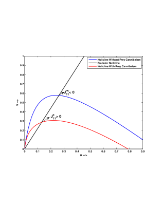
We can also take a geometric approach similar to Fasani [10] to proceed. We investigate the nullclines of (11), shown in fig. 5.

Figure 5. Here we see the nullclines of the model (11) vs the nullclines of model (12). We see prey cannibalism drives down the prey nullcline.

Remark 7.

Since the situation in fig. 5 is clearly achievable geometrically, there is a chance that prey cannibalism could bring about Turing instability, even if $\beta<\frac{1}{(\sqrt{1-\alpha})(1+\sqrt{1-\alpha})}$. We then perform a parameter sweep based on the Turing conditions that we derive, in order to see if the appropriate parameters can be found.

4.2. Turing instability due to prey cannibalism

For details on the Turing calculations we refer the reader to [36]. The calculations therein yield various necessary and sufficient conditions for Turing instability to occur, if prey cannibalism is present. We state our result via the following theorem.

Theorem 4.3 ( Prey cannibalism induced Turing Instability).

Consider $(u_{c},v_{c})$ which is a spatially homogenous equilibrium point of the model system (12). If there exist parameters $(\alpha,\beta,c,d,c_{1})$ all strictly positive, s.t at $(u_{c},v_{c})$, the Jacobian $\mathbf{J}=\begin{bmatrix}J_{11}&J_{12}\\ J_{21}&J_{22}\end{bmatrix}$, and the diffusion coefficients $D_{u},D_{v}$ satisfy

$$\left(\dfrac{\beta}{\left(1+\alpha\beta\right)^{2}}-u_{c}\right)\dfrac{\left(u_{c}+d\right)^{2}}{du_{c}}>{c}>\left(\dfrac{\beta}{\left(1+\alpha\beta\right)^{2}}-u_{c}-\delta\beta\right)\dfrac{\left(u_{c}+d\right)^{2}}{du_{c}}$$

$$\left(D_{v}\left(\frac{\beta}{\left(1+\alpha\beta\right)^{2}}-u_{c}-\frac{cdu_{c}}{\left(u_{c}+d\right)^{2}}\right)-D_{u}\beta\delta\right)>0$$

$$\left(D_{v}\left(\frac{\beta}{\left(1+\alpha\beta\right)^{2}}-u_{c}-\frac{cdu_{c}}{\left(u_{c}+d\right)^{2}}\right)-D_{u}\beta\delta\right)>2\sqrt{D_{u}D_{v}\left(\tfrac{\left(\beta\delta d^{2}u_{c}+2\beta\delta d(u_{c})^{2}+c\beta\delta du_{c}+\beta\delta(u_{c})^{3}\right)\allowbreak}{d^{2}+2du_{c}+(u_{c})^{2}}\right)},$$

$$\beta\leq\frac{1}{(\sqrt{1-\alpha})(1+\sqrt{1-\alpha})},$$

then $(u_{c},v_{c})$ is linearly stable in the absence of diffusion and linearly unstable in the presence of diffusion, whilst $(u_{nc},v_{nc})$ which is a spatially homogenous equilibrium point of the model system (11) is linearly stable in the presence of diffusion, for the same parameters $(\alpha,\beta,d)$, and $c=c_{1}=0$. That is, in the absence of prey cannibalism.

Remark 8.

Note for system (12) and for (11) we have that $J_{11}J_{22}-J_{21}J_{12}>0$.

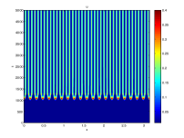
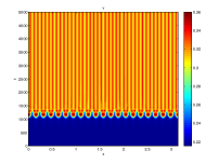
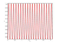
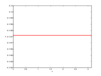
A parameter sweep using the above conditions yields that such a parametric space is definitely possible. For chosen parameters in this space, we see Turing patterns as in fig. 6.

Figure 6. Here the Turing patterns in predator and prey, are shown for model (12), that is when there is prey cannibalism. Spatial patterns are formed. In these simulations $\Omega=[0,\pi]$, and the spatially homogenous steady state is given a small perturbation by a function of the form $\epsilon_{1}cos^{2}(10x)$, $\epsilon_{1}<<1$. For the parameters used please see Table 1.

Figure 7. Here the model (12) (that is when there is prey cannibalism), is contrasted with model (11). We see in Fig (a) (model (12)) the density of the prey at time t=5000. There is a spatial pattern. In Fig (b) (model (11)) there is no pattern. For the parameters used please see Table 1.

Now we move in the opposite direction. Supposing that the conditions of theorem 4.3 do not hold, and we do not have Turing instability in the nc model (12). Can removing the prey cannibalism bring about Turing instability? We next provide a sufficient condition under which this is not possible. This is done via the following lemma

Lemma 4.4.

Consider $(u^{c},v^{c})$ which is a spatially homogenous equilibrium point of the model system (12) which is linearly stable both in the absence of diffusion and in the presence of diffusion. If $J^{c}_{11}<0$ or $\left(\left(\dfrac{\beta}{\left(1+\alpha\beta\right)^{2}}-u^{c}\right)\left(u^{c}+d\right)^{2}\right)\dfrac{1}{u^{c}}<cd$, and if $m+d+c\leq 1+c_{1}$, and $1-\frac{\beta}{1+\alpha\beta}<\frac{1}{2+\alpha\beta}$. Then $(u^{nc},v^{nc})$ which is a spatially homogenous equilibrium point of the model system (11), for the same parameter set, but when $c=c_{1}=0$, is also linearly stable in the presence of diffusion

Proof.

The proof follows via observing that if

$$\left(\left(\dfrac{\beta}{\left(1+\alpha\beta\right)^{2}}-u^{c}\right)\left(u^{c}+d\right)^{2}\right)\dfrac{1}{u^{c}}>cd$$

$$=>\dfrac{\beta}{\left(1+\alpha\beta\right)^{2}}<u^{c}+\frac{cdu^{c}}{\left(u^{c}+d\right)^{2}}<u_{nc}$$

$$=1-\frac{\beta}{1+\alpha\beta}<\frac{1}{2+\alpha\beta}$$

This implies that $\beta(\alpha\beta+2)<(1+\alpha\beta)^{2}$, which in turn implies that $\beta<\frac{1}{(\sqrt{1-\alpha})(1+\sqrt{1-\alpha})}$, and so Turing instability is an impossibility in (11), from lemma 4.2. Note $u^{c}+\frac{cdu^{c}}{\left(u^{c}+d\right)^{2}}<u_{nc}$ follows from the assumption $m+d+c\leq 1+c_{1}$, and lemma 2.3. ∎

Remark 9.

Essentially removing prey cannibalism, shifts the prey null cline up, still leaving $J^{nc}_{11}<0$, at the new equilibrium $(u^{nc},v^{nc})$. This is easily seen in fig. 5.

We lastly state a result concerning Turing pattern formation and predator cannibalism

Lemma 4.5.

The equilibrium point $\left(u_{nc},v_{nc}\right)$ cannot be driven unstable via diffusion, in the presence of predator cannibalism, if and $\gamma<\frac{\beta}{\beta_{1}}$. However, if $\gamma>\frac{\beta}{\beta_{1}}$, then $\left(u_{nc},v_{nc}\right)$ can be driven unstable via diffusion, in the presence of predator cannibalism.

Proof.

The proof is an immediate consequence of the null cline analysis. If $J^{nc}_{11}=\beta\leq\frac{1}{(\sqrt{1-\alpha})(1+\sqrt{1-\alpha})}<0$, Turing instability is an impossibility. However, predator cannibalism will only push the null cline further to the right if $\gamma<\frac{\beta}{\beta_{1}}$, and so $J^{c}_{11}<0$, thus Turing patterns are an impossibility, in this case. However, if $\gamma>\frac{\beta}{\beta_{1}}$, then predator cannibalism will push the predator null cline to the left, and it is possible that $J^{c}_{11}>0$, so that Turing patterns could occur. ∎

5. Dynamics of the PDE model with noise

In mathematical modeling, deterministic systems of PDEs have been relied upon to capture the relevant dynamics of some biological systems. However, these systems are frequently subject to noisy environments, inputs and signalling. It was reported that songbirds experience decreased predation rate in the environments with noise [11], and hermit crabs were distracted by boat motor noise and hence less vigilant against approaching predators [6, 30]. Thus stochastic perturbations are important when considering the ability of such models to reproduce results consistently. In particular, owing to the Turing mechanism being very sensitive to perturbations, stochasticity is able to affect evolving patterns in ways not seen in deterministic simulations [20].

Previous result in stochastic predator-prey models focused on internal noise[19, 15, 33], where it is assumed that noise affect the model system itself. This allows to account for such fluctuations even in the framework of a continuum model [15]. However, predator-prey models with Holling type II external noise had been generally overlooked despite its potential ecological reality and theoretical interest. Recent theoretical work indicates that cannibalism can strongly promote coexistence between a prey and a predator, especially if the mortality rate due to cannibalism is sufficiently larger than the heterospecific predation rate [27], as a result, we investigate the effect of external spatial temporal noise on Turing patterns in a predator-prey model with diffusion and Holling type II functional response, with prey cannibalism. We model these perturbations as said, by means of independent Gaussian white noises.

In this present paper, we only assume some control parameter of the system is affected by environmental fluctuations such as epidemics, weather and nature disasters. We consider fluctuations presented in by the coefficient of the cannibalistic term of the prey, which is define as mortality rate due to cannibalism. Hence by introducing a stochastic factor both in space and time ${\mathrm{\eta}(x,t)}$ into the coefficient of the cannibalistic term $(c)$, the parameter $c$ is treated as a Guassian random variable with mean $\hat{c}$ and intensity $\epsilon$.

(16) $$c\rightarrow{\hat{c}}+\epsilon{\mathrm{\eta}(x,t)},$$

We therefore introduce equation (16) in order to extend model system (12) such that we obtain a system of It$\hat{o}^{\prime}s$ stochastic differential equations in the form, where for simplicity, we redefine mean $\hat{c}$ to be the parameter $c$. :

(17a) $${\frac{\partial u}{\partial t}}=D_{u}\Delta u+u(1+c_{1}-u)-{\frac{uv}{u+\alpha v}}-{\frac{cu^{2}}{u+d}}-{\frac{\epsilon u^{2}}{u+d}}{\mathrm{\eta}(x,t)},$$

(17b) $${\frac{\partial v}{\partial t}}=D_{v}\Delta v+\delta v\left(\beta-\frac{v}{u}\right).$$

5.1. Numerical Experiment

In this section, we discretize numerically the stochastic predator-prey model (17) with white noise. We redefine the noise term ${\mathrm{\eta}(x,t)}$ as ${\mathrm{\partial}^{2}W(x,t)/\partial x\partial t}$, where $W(x,t)$ is a one-dimensional Brownian motion. The spatial approximation is constructed from a Chebychev collocation scheme[13, 9]. Thus the spatial approximation is constructed as a linear combination of the interpolating splines on the Gauss-Lobatto quadrature ${x_{j}}$, with a spatial domain size of N=256. This reduces model system (12) to a system of It$\hat{o}^{\prime}s$ stochastic ordinary differential equation. The resulting system is then integrated in time using an implicit Milsten scheme for approximating It$\hat{o}^{\prime}s$ stochastic ordinary differential equation, with a time stepsize of $\Delta t=0.1$. This therefore reduce the It$\hat{o}^{\prime}s$ stochastic ordinary differential equation to the form

(18) $$\begin{split}{\bf{u}}^{n+1}_{j}-{\bf{u}}^{n}_{j}&=\bigg{(}D_{u}\sum_{i=1}^{N-1}{\bf{D^{2}}}_{ji}{\bf{u}}^{n+1}_{i}+{\bf{u}}^{n+1}_{j}(1+c_{1}-{\bf{u}}^{n+1}_{j})-{{\bf{u}}^{n+1}_{j}{\bf{v}}^{n+1}_{j}\over{\bf{u}}^{n+1}_{j}+\alpha{\bf{v}}^{n+1}_{j}}-{c({\bf{u}}^{n+1}_{j})^{2}\over{\bf{u}}^{n+1}_{j}+d}\bigg{)}\Delta t\\ &\quad\quad\quad\quad\quad\quad\quad\quad\quad\quad-{\epsilon({{\bf{u}}^{n}_{j}})^{2}\over{\bf{u}}^{n}_{j}+d}{\mathrm{\Delta}W_{j}}-{\epsilon^{2}\over 2}{({{\bf{u}}^{n}_{j}})^{3}({\bf{u}}^{n}_{j}+2d)\over({\bf{u}}^{n}_{j}+d)^{3}}\bigg{(}(\Delta W_{j})^{2}-\Delta t\bigg{)},\end{split}$$

(19) $${\bf{v}}^{n+1}_{j}-{\bf{v}}^{n}_{j} =\left(D_{v}\sum_{i=1}^{N-1}{\bf{D^{2}}}_{ji}{\bf{v}}^{n+1}_{i}+\delta{\bf{v}}^{n+1}_{j}\left(\beta-\frac{{\bf{v}}^{n+1}_{j}}{{\bf{u}}^{n+1}_{j}}\right)\right)\Delta t,$$

where $\mathbf{D^{2}}_{ji}$ is known as the 2nd order spectral differentiation matrix and $\mathbf{u}^{n}_{j}=u(x_{j},t_{n})$, whereas $\mathbf{v}^{n}_{j}=v(x_{j},t_{n})$, for $j=1,\ldots,N-1$. Also $\Delta W_{j}=z_{j}\sqrt{\Delta t}$, where $z_{j}\sim\mathcal{N}(0,1)$ is normally distributed random numbers with mean 0 and standard deviation 1.
The implicit Milsten scheme used to advance the initial value problem in time necessitates solving a nonlinear system of equations at each time step. This is achieved through a Newton-Raphson method.

5.2. The effect of Noisy cannibalism rate on Turing Instability

In this section we investigate numerically by simulation the effects of noise on Turing patterns at time $t=5000$. Extensive testing was performed through numerical integration to describe model (17), and the results are shown in this section. This is done by using an initial condition defined in a small perturbation around the positive homogenous steady state given, which is as

$$u=u^{*}+\alpha_{1}cos^{2}(nx)(x>0)(x<\pi),$$

$$v=v^{*}+\alpha_{2}cos^{2}(nx)(x>0)(x<\pi),$$

where $\alpha_{1}=0.0002$ and $\alpha_{2}=0.02.$ During the simulations, different types of dynamics are obtained for both the prey and predator. Consequently in this section, we can restrict our analysis of pattern formation to prey population $u$ since much of the noise in model system (17) affect the prey population.
In our numerical simulation with a specific parameter set in the Turing domain as show in Fig.(8), we show the evolution of fixed spatial pattern of prey population from deterministic model (model system (12)) to stochastic model (model system (17)) where with noise we consider $\epsilon=0.1$ and $0.4$ with small random perturbation of the stationary solution $(u^{*},v^{*})$ as given above. It is numerically evidenced from Fig.(8) (first plot $\epsilon=0$, middle plot $\epsilon=0.1$ and last plot $\epsilon=0.4$) that large variety of distinct patterns can be obtained by making small changes to the level of intensity $\epsilon$ in the stochastic model, which can also cause the disappears of Turing patterns as well as the pattern formed can be enhance by small intensity levels. Therefore in our experiments it was realized that for a given parameter set in the Turing domain, there exist a specific intensity $\epsilon$ level of the noise that can cause the average prey population species to decrease significantly as well as the disappearance of pattern formation.

Figure 8.

We next investigate whether noise can induce pattern formation. This achieved by using a non-Turing parameter set. Fig.(9) shows the dynamic behavior of model (17) with non-Turing parameter set. The first plot of Fig.(9) shows the plot of the deterministic model where with diffusion the prey population still goes into a steady state(hence no Turing Patterns formed), the proceeding plot of Fig.(9) shows the evolution from non-Turing patterns to some form of weak patterns as $\epsilon$ changes from $\epsilon=0.1$ to $\epsilon=0.4$.

Figure 9.

Clearly from above, it is comprehensible that noise can induce instability, and the effect of noise on model system (17) is drastic. Thus noise can enhance, as well as cause the disappearance of patterns formed in the deterministic model. These behaviors confirm how sensitive model system (17) is to different noise intensities.

Table 1. Parameters used in the simulations. In all figures.

Fig.	$\alpha$	$\beta$	$c_{1}$	$c$	$d$	$\delta$	$D_{u}$	$D_{v}$
2,3,4	0.73	5.21	0.25	1.0	0.11	0.013	0.0	0.0
5	0.9	2.2	0.01	0.25	0.1	0.1	0.0	0.0
6,7a	1.0	7.35	0.01	0.17	0.01	0.32	$10^{-5}$	$10^{-2}$
7b	1.0	7.35	0.0	0.0	0.00	0.32	$10^{-5}$	$10^{-2}$
8	1.0	2.72	0.01	0.17	0.01	0.32	$10^{-5}$	$10^{-2}$
9	1.05	7.34	0.01	0.2	0.1	0.32	$10^{-5}$	$10^{-2}$

6. Discussion and Conclusion

Cannibalism, although ubiquitous in both predator and prey communities, has primarily been studied as a phenomenon in the predator species. In the current manuscript we have considered the effect of both predator and prey cannibalism on a Holling Tanner model, with ratio dependent functional response. Our results show that in the ODE version of the model, in certain parameter regime, predator cannibalism is able to stabilize the unstable interior equilibrium, (that is the equilibrium is unstable if there is no cannibalism). This stability result depends critically on the cannibals feeding rate of prey $\gamma$, and the ratio $\dfrac{\beta}{\beta_{1}}$. That is if the cannibalistic predator eats less prey so $\gamma$ is small in comparison to $\dfrac{\beta}{\beta_{1}}$, then only a little bit of feeding of conspecifics is enough to stabilize the dynamics. This is seen via lemma 2.1, and is in accordance with known facts about predator cannibalism in other models. However, when we consider prey cannibalism, we see that it is not able to stabilize the unstable interior equilibrium. This is rigorously proven for small prey cannibalism rate $c$, via lemma 2.3. We conjecture this is true even for large cannibalism rate.

This result tells us that for parameters such that the no cannibalism model (11) has an unstable equilibrium, or essentially cyclical dynamics, no amount of prey cannibalism can stabilize this. From an ecological perspective, this tells us that in a predator-prey community with cyclical fluctuation in the predator and prey populations (so essentially limit cycle dynamics), cannibalism in the prey would just maintain the cyclically, and the oscillations in population cannot be driven to a stable steady state. Interestingly, this is seen to hold even if we assume some stochasticity in the prey cannibalism rate, see figs. 2-4.

We also see that prey cannibalism can lead to limit cycle dynamics, but the uniqueness or non uniqueness of limit cycles is an open question. It would be extremely interesting to investigate this further. In particular one may ask, if changing the form of the prey cannibalism term $C(u)$ may lead to multiple limit cycles, or render the limit cycle unique. Another interesting open problem, would be to consider the effect of both predator and prey cannibalism together, on models of Holling Tanner type. In particular, one might try to classify regions, where they have conflicting effects, that is say predator cannibalism stabilises while prey cannibalism destabilises, and to then consider the net effect, in terms of the parameters concerned. To the best of our knowledge, this has not been considered in any work in the literature. Also, of much interest lately is the problem of a diseased predator in predator-prey models with cannibalistic predators. It is seen that cannibalism in the predator, can prevent disease in predator from spreading, as the cannibal could wipe out the diseased predator [3]. It would be interesting to consider such a system, with cannibalism now in the prey, and also a diseased prey. Here one can ask if prey cannibalism could stop disease in the prey species, as is known from similar models in predator cannibalism.

In case of the spatially explicit model, we uncover certain interesting results as well. What we observe is that for small predator growth rate, or if prey handling time and prey capture rate are close, Turing patterns are an impossibility in the no cannibalism model. That is spatial segregation cannot occur in (11). However, even if one maintains this small predator growth rate, or if prey handling time and prey capture rate are close, if the prey cannibalism rate is chosen in the right regime, see theorem 4.3, then one can still have spatial patterns in the prey cannibalism model (12). From a spatial ecology perspective this is quite interesting, as this is telling us that if the predator growth rate is curtailed for some reason, in the Holling Tanner model, spatial segregation cannot occur, unless prey cannibalism takes place, in which case spatial segregation can occur. Interestingly, if one compares the destabilizing influence of prey cannibalism in the ODE and PDE models, we find that if the cannibalism rate $c<2(u_{nc}-u_{c})$, then it will destabilize in the ODE case. However, to destabilize in the PDE case, it cannot be “to small”, and must be such that

$$\left(\dfrac{\beta}{\left(1+\alpha\beta\right)^{2}}-u_{c}\right)\dfrac{\left(u_{c}+d\right)^{2}}{du_{c}}>{c}>\left(\dfrac{\beta}{\left(1+\alpha\beta\right)^{2}}-u_{c}-\delta\beta\right)\dfrac{\left(u_{c}+d\right)^{2}}{du_{c}}$$

as seen in theorem 4.3. Alternatively, we show that predator cannibalism cannot cause Turing patterns if the predator feeding rate is curtailed, according to the parametric restriction $\gamma<\frac{\beta}{\beta_{1}}$, as seen in lemma 4.5.

Lastly, ecosystems are always subject to random forcing. However there have been no studies with a random cannibalism rate, even as far as predator cannibalism goes, let alone prey cannibalsim. Our results with a random cannibalism rate show that it can affect both limit cycle dynamics, as well as completely alter the spatial Turing patterns, that form in the deterministic case, see figs. 8-9. In case of limit cycle dynamics, noisy cannibalism makes things aperiodic, but cannot remove the population cycles completely. In the case of the spatially explicit model, the noise is seen to both be able to create patterns, as well as to destroy them.

All in all, we hope that the current work leads to many further investigations, into the fascinating effects of prey cannibalism on predator prey dynamics. Such endeavours will bring us closer to understanding the full extent of cannibalism as it occurs in nature, and the role it plays in shaping predator-prey communities.

7. Acknowledgements

We would like to acknowledge very helpful conversations with Professor Volker Rudolf, in the department of Biosciences at Rice University, on various ecological concepts of prey cannibalism, and its mathematical modeling.

References

- [1] Peter A Abrams and Lev R Ginzburg. The nature of predation: prey dependent, ratio dependent or neither? Trends in Ecology & Evolution, 15(8):337–341, 2000.
- [2] Malay Banerjee and Santo Banerjee. Turing instabilities and spatio-temporal chaos in ratio-dependent holling–tanner model. Mathematical biosciences, 236(1):64–76, 2012.
- [3] Santosh Biswas, Samrat Chatterjee, and Joydev Chattopadhyay. Cannibalism may control disease in predator population: result drawn from a model based study. Mathematical Methods in the Applied Sciences, 2014.
- [4] B Buonomo, D Lacitignola, and S Rionero. Effect of prey growth and predator cannibalism rate on the stability of a structured population model. Nonlinear Analysis: Real World Applications, 11(2):1170–1181, 2010.
- [5] Bruno Buonomo and Deborah Lacitignola. On the stabilizing effect of cannibalism in stage-structured population models. Mathematical biosciences and engineering: MBE, 3(4):717–731, 2006.
- [6] Alvin Aaden Yim-Hol Chan, Paulina Giraldo-Perez, Sonja Smith, and Daniel T Blumstein. Anthropogenic noise affects risk assessment and attention: the distracted prey hypothesis. Biology Letters, 6(4):458–461, 2010.
- [7] Yunshyong Chow and Sophia R-J Jang. Cannibalism in discrete-time predator–prey systems. Journal of biological dynamics, 6(1):38–62, 2012.
- [8] David Claessen, Andre M De Roos, and Lennart Persson. Population dynamic theory of size–dependent cannibalism. Proceedings of the Royal Society of London B: Biological Sciences, 271(1537):333–340, 2004.
- [9] Wai Sun Don and Alex Solomonoff. Accuracy and speed in computing the chebyshev collocation derivative. SIAM Journal on Scientific Computing, 16(6):1253–1268, 1995.
- [10] Stefano Fasani and Sergio Rinaldi. Remarks on cannibalism and pattern formation in spatially extended prey–predator systems. Nonlinear Dynamics, 67(4):2543–2548, 2012.
- [11] Clinton D Francis, Catherine P Ortega, and Alexander Cruz. Noise pollution changes avian communities and species interactions. Current biology, 19(16):1415–1419, 2009.
- [12] Ph Getto, O Diekmann, and AM De Roos. On the (dis) advantages of cannibalism. Journal of mathematical biology, 51(6):695–712, 2005.
- [13] David Gottlieb and Liviu Lustman. The spectrum of the chebyshev collocation operator for the heat equation. SIAM journal on numerical analysis, 20(5):909–921, 1983.
- [14] Sze-Bi Hsu and Tzy-Wei Huang. Global stability for a class of predator-prey systems. SIAM Journal on Applied Mathematics, 55(3):763–783, 1995.
- [15] Jan Kelkel and Christina Surulescu. On a stochastic reaction–diffusion system modeling pattern formation on seashells. Journal of mathematical biology, 60(6):765–796, 2010.
- [16] Debra Kelly. The culture that still practices cannibalism, October 2013.
- [17] C Kohlmeier and W Ebenhöh. The stabilizing role of cannibalism in a predator-prey system. Bulletin of Mathematical Biology, 57(3):401–411, 1995.
- [18] PH Leslie and JC Gower. The properties of a stochastic model for the predator-prey type of interaction between two species. Biometrika, pages 219–234, 1960.
- [19] Li Li and Zhi-Jun Wang. Dynamics in a predator–prey model with space and noise. Applied Mathematics and Computation, 219(12):6542–6547, 2013.
- [20] Philip K Maini, Thomas E Woolley, Ruth E Baker, Eamonn A Gaffney, and S Seirin Lee. Turing’s model for biological pattern formation and the robustness problem. Interface focus, page rsfs20110113, 2012.
- [21] James D Murray. Mathematical biology i: An introduction, vol. 17 of interdisciplinary applied mathematics, 2002.
- [22] Akira Okubo and Smon A Levin. Diffusion and ecological problems: modern perspectives, volume 14. Springer Science & Business Media, 2013.
- [23] CR Pennell. Cannibalism in early modern north africa. British Journal of Middle Eastern Studies, 18(2):169–185, 1991.
- [24] Gary A Polis. The evolution and dynamics of intraspecific predation. Annual Review of Ecology and Systematics, pages 225–251, 1981.
- [25] Associated Press. Indian doc focuses on hindu cannibal sect, October 2005.
- [26] Volker HW Rudolf. Consequences of stage-structured predators: cannibalism, behavioral effects, and trophic cascades. Ecology, 88(12):2991–3003, 2007.
- [27] Volker HW Rudolf. The interaction of cannibalism and omnivory: consequences for community dynamics. Ecology, 88(11):2697–2705, 2007.
- [28] Volker HW Rudolf. The impact of cannibalism in the prey on predator-prey systems. Ecology, 89(11):3116–3127, 2008.
- [29] Moitri Sen, Malay Banerjee, and Andrew Morozov. Bifurcation analysis of a ratio-dependent prey–predator model with the allee effect. Ecological Complexity, 11:12–27, 2012.
- [30] Björn M Siemers and Andrea Schaub. Hunting at the highway: traffic noise reduces foraging efficiency in acoustic predators. Proceedings of the Royal Society of London B: Biological Sciences, 278(1712):1646–1652, 2011.
- [31] Francisco J Solis and Roberto A Ku-Carrillo. Birth rate effects on an age-structured predator-prey model with cannibalism in the prey. In Abstract and Applied Analysis, volume 501, page 241312. Hindawi Publishing Corporation, 2014.
- [32] Steven H Strogatz. Nonlinear dynamics and chaos: with applications to physics, biology, chemistry, and engineering. Westview press, 2014.
- [33] Gui-Quan Sun, Zhen Jin, Quan-Xing Liu, and Bai-Lian Li. Rich dynamics in a predator–prey model with both noise and periodic force. BioSystems, 100(1):14–22, 2010.
- [34] Gui-Quan Sun, Guang Zhang, Zhen Jin, and Li Li. Predator cannibalism can give rise to regular spatial pattern in a predator–prey system. Nonlinear Dynamics, 58(1-2):75–84, 2009.
- [35] Alan Mathison Turing. The chemical basis of morphogenesis. Philosophical Transactions of the Royal Society of London B: Biological Sciences, 237(641):37–72, 1952.
- [36] KAJ White and CA Gilligan. Spatial heterogeneity in three species, plant–parasite–hyperparasite, systems. Philosophical Transactions of the Royal Society B: Biological Sciences, 353(1368):543–557, 1998.
- [37] Limin Zhang and Chaofeng Zhang. Rich dynamic of a stage-structured prey–predator model with cannibalism and periodic attacking rate. Communications in Nonlinear Science and Numerical Simulation, 15(12):4029–4040, 2010.