Optimal Piecewise Linear Function Approximation for GPU-based Applications

Abstract

Many computer vision and human-computer interaction applications developed in recent years need evaluating complex and continuous mathematical functions as an essential step toward proper operation. However, rigorous evaluation of this kind of functions often implies a very high computational cost, unacceptable in real-time applications. To alleviate this problem, functions are commonly approximated by simpler piecewise-polynomial representations. Following this idea, we propose a novel, efficient, and practical technique to evaluate complex and continuous functions using a nearly optimal design of two types of piecewise linear approximations in the case of a large budget of evaluation subintervals. To this end, we develop a thorough error analysis that yields asymptotically tight bounds to accurately quantify the approximation performance of both representations. It provides an improvement upon previous error estimates and allows the user to control the trade-off between the approximation error and the number of evaluation subintervals. To guarantee real-time operation, the method is suitable for, but not limited to, an efficient implementation in modern Graphics Processing Units (GPUs), where it outperforms previous alternative approaches by exploiting the fixed-function interpolation routines present in their texture units. The proposed technique is a perfect match for any application requiring the evaluation of continuous functions; we have measured in detail its quality and efficiency on several functions, and, in particular, the Gaussian function because it is extensively used in many areas of computer vision and cybernetics, and it is expensive to evaluate.

I Introduction

The design of high-quality and real-time image processing algorithms is a key topic in today’s context, where humans demand more capabilities and control over their rapidly increasing number of advanced imaging devices such as cameras, smart phones, tablets, etc. [1]. Many efforts are being made toward satisfying those needs by exploiting dedicated hardware, such as Graphics Processing Units (GPUs) [2, 3, 4]. Some areas where GPUs are emerging to improve Human Computer Interaction (HCI) include cybernetics (for example, in facial [5] or object [6] recognition, classification using Support Vector Machines [7] and genetic algorithms for clustering [8]), and image processing (e.g., unsupervised image segmentation [3, 9], optical coherence tomography systems [4], efficient surface reconstruction from noisy data [10], remote sensing [11], real-time background subtraction [12], etc.). In such hardware-oriented designed algorithms, the computational efficiency of processing tasks is significantly improved by parallelizing the operations.

(a)

(b)

Figure 1: High level tasks such as (a) object/person-tracking or (b) video-based gestural interfaces often require a foreground segmentation method as a base building block.

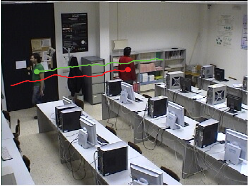
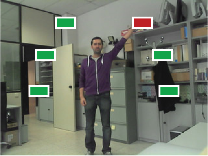
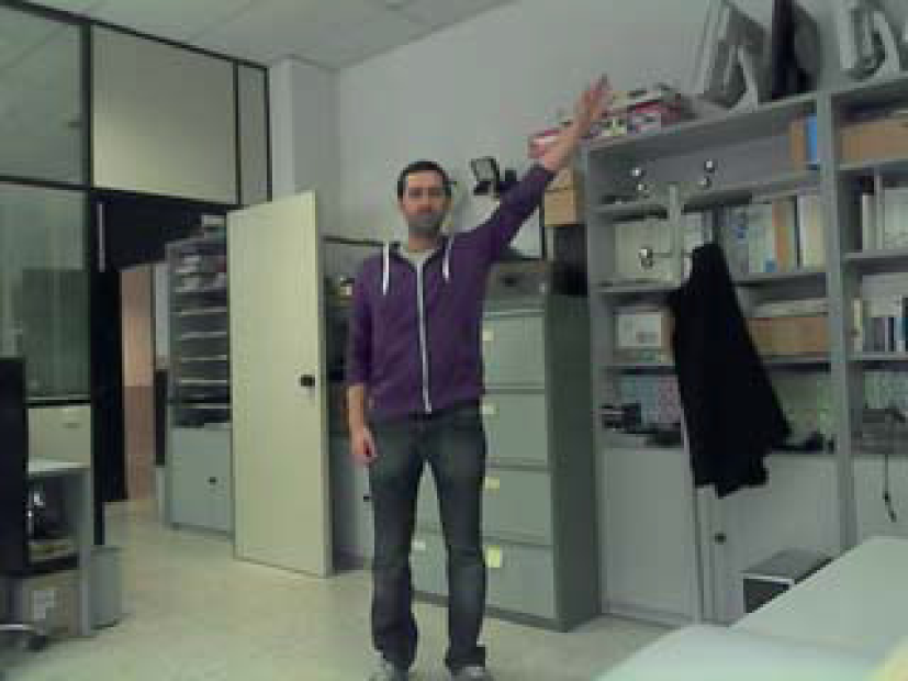
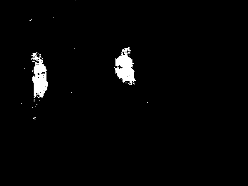
Automated video analysis applications such as person tracking or video-based gestural interfaces (see Figure 1) rely on lower-level building blocks like foreground segmentation [13, 14], where the design of efficient computational methods for dedicated hardware has a significant impact. Multimodal nonparametric segmentation strategies have drawn a lot of attention [15, 16] since they are able to provide high-quality results even in complex scenarios (dynamic background, illumination changes, etc.) [17]. However, their main drawback is their extremely high computational cost (requiring the evaluation of billions of multidimensional Gaussian kernels per second), which makes them difficult to integrate in the latest generation of image processing applications [18, 19]. To overcome this important drawback and achieve real-time performance [20], the use of parallel hardware such as GPUs helps but may not be enough by itself, depending on the required resolution, hence the need for algorithms capable of evaluating non-linear (e.g., Gaussian) functions at high speed within a required error tolerance. GPU vendors are aware of this recurrent computing problem and provide hardware implementations of common transcendental functions in Special Function Units (SFUs) [21]; indeed, we can find in the literature examples of successful use of these hardware facilities [22]. However, their ease of use comes at the price of non-customizable reduced numerical precision [23].

I-A Contribution

We propose a novel, fast, and practical method to evaluate any continuous mathematical function within a known interval. Our contributions include, based on error equalization, a nearly optimal design of two types of piecewise linear approximations (linear interpolant and orthogonal projection) in the $L_{2}$ norm under the constraint of a large budget of evaluation subintervals $N$. Moreover, we provide asymptotically tight bounds for the approximation errors of both piecewise linear representations, improving upon existing ones. Specifically, in addition to the $O(N^{-2})$ convergence rate typical of these approximations, we quantify their interpolation constants: $1/\sqrt{120}$ for the linear interpolant and a further $\sqrt{6}$ improvement factor in case of the orthogonal projection. The obtained error relations are parameterized by the number of segments used to represent the complex (nonlinear) function, hence our approach allows the user to estimate the errors given $N$ or, conversely, estimate the required $N$ to achieve a target approximation error.

We also propose an efficient implementation of the technique in a modern GPU by exploiting the fixed-function interpolation routines present in its texture units to accelerate the computation while leaving the rest of the GPU (and, of course, the CPU) free to perform other tasks; this technique is even faster than using SFUs [21].

Although the initial motivation of the developed method was to improve the efficiency of nonparametric foreground segmentation strategies, it must be noted that it can be also used in many other scientific fields such as computer vision [24, 25] or audio signal processing [26, 27], where the evaluation of continuous mathematical functions constitutes a significant computational burden.

I-B Organization

Section II summarizes the basic facts about piecewise linear approximation of real-valued univariate functions and reviews related work in this topic; Section III derives a suboptimal partition of the domain of the approximating function in order to minimize the distance to the original function (proofs of results are given in the Appendixes); Section IV analyzes the algorithmic complexity of the proposed approximation strategies and Section V gives details about their implementation on modern GPUs. Section VI presents the experimental results of the proposed approximation on several functions (Gaussian, Lorentzian and Bessel’s), both in terms of quality and computational times, and its use is demonstrated in an image processing application. Finally, Section VII concludes the paper.

II Piecewise Linear Modelization

II-A Related Work

In many applications, rigorous evaluation of complex mathematical functions is not practical because it takes too much computational power. Consequently, this evaluation is carried out approximating them by simpler functions such as (piecewise-)polynomial ones. Piecewise linearization has been used as an attractive simplified representation of various complex nonlinear systems [28]. The resulting models fit into well established tools for linear systems and reduce the complexity of finding the inverse of nonlinear functions [29, 30]. They can also be used to obtain approximate solutions in complex nonlinear systems, for example, in Mixed-Integer Linear Programming (MILP) models [31]. Some efforts have been devoted as well to the search for canonical representations in one and multiple dimensions [32, 33] with different goals such as black box system identification, approximation or model reduction.

Previous attempts to address the problem considered here (optimal function piecewise linearization) include [34, 35, 29, 36], the latter two in the context of nonlinear dynamical systems. In [34] an iterative multi-stage procedure based on dynamical programming is given to provide a solution to the problem on sequences of progressively finer 2-D grids. In [29] the piecewise linear approximation is obtained by using the evolutionary computation approach such as genetic algorithm and evolution strategies; the resulting model is obtained by minimization of a sampled version of the mean squared error and it may not be continuous. In [36] the problem is addressed using a hybrid approach based on curve fitting, clustering and genetic algorithms. Here we address the problem from a less heuristic point of view, using differential calculus to derive a more principled approach [37]. Our method solely relies on standard numerical integration techniques, which takes few seconds to compute, as opposed to recursive partitioning techniques such as [35], which take significantly longer.

II-B Basic Results in Piecewise-Linear Interpolation and Least-Squares Approximation

In this section we summarize the basic theory behind piecewise linear functions [38] and two such approximations to real-valued functions: interpolation and projection (Sections II-B1 and II-B2, respectively), pictured in Figure 2 along with their absolute approximation error with respect to $f$.

Figure 2: Top: fifth-degree polynomial $f(x)=(x+4)(x+2)(x+1)(x-1)(x-3)$ and two continuous piecewise linear (CPWL) approximations, the orthogonal projection $P_{T}f$ and the linear interpolant $\pi_{T}f$; bottom: corresponding absolute approximation errors (magnified by a $5\times$ factor).

Figure 3: Hat functions constitute a basis of $\mathrm{V}_{T}$. Since all the basis functions are zero outside $I=[a,b]$, the basis functions associated with boundary nodes are only half hats.

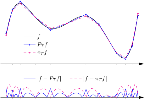
In essence, a piecewise function over an interval $I=\left[a,b\right]$ is a partition of $I$ into a set of $N$ subintervals $T=\{I_{i}\}_{i=1}^{N}$, where $I_{i}=\left(x_{i-1},x_{i}\right)\mid a=x_{0}<x_{1}<\ldots<x_{N}=b$, and a set of $N$ functions $f_{i}(x)$, one for each subinterval $I_{i}$. In particular we are interested in continuous piecewise linear (CPWL) functions, which means that all the $f_{i}(x)$ are linear and $f_{i}(x_{i})=f_{i+1}(x_{i})\;\forall i=\left\{1,\ldots,N-1\right\}$. CPWL functions of a given partition $T$ are elements of a vector space $\mathrm{V}_{T}$: the addition of such functions and/or multiplication by a scalar yields another CPWL function defined over the same subintervals. A useful basis for the vector space $\mathrm{V}_{T}$ is formed by the set of hat functions or nodal basis functions $\left\{\varphi_{i}\right\}_{i=0}^{N}$, pictured in Figure 3 and defined in general by the formula

$$\varphi_{i}(x)=\begin{cases}(x-x_{i-1})/(x_{i}-x_{i-1}),&x\in\left[x_{i-1},x_{i}\right]\\ (x-x_{i+1})/(x_{i}-x_{i+1}),&x\in\left[x_{i},x_{i+1}\right]\\ 0,&x\notin\left[x_{i-1},x_{i+1}\right].\end{cases}$$ (1)

The basis functions $\varphi_{0}$ and $\varphi_{N}$ associated to the boundary nodes $x_{0}$ and $x_{N}$ are only half hats.

These basis functions are convenient since they can represent any function $v$ in $\mathrm{V}_{T}$ by just requiring the values of $v$ at its nodal points, $v(x_{i})$, in the form

$$v(x)=\sum_{i=0}^{N}v(x_{i})\varphi_{i}(x).$$ (2)

II-B1 Linear Interpolation

The piecewise linear interpolant $\pi_{T}f\in\mathrm{V}_{T}$ of a continuous function $f$ over the interval $I$ can be defined in terms of the basis just introduced:

$$\pi_{T}f(x)=\sum_{i=0}^{N}f(x_{i})\varphi_{i}(x).$$ (3)

While this CPWL approximation is trivial to construct, and may be suitable for some uses, it is by no means the best possible one. Crucially, $\pi_{T}f(x)\geq f(x)\;\forall x\in I$ for any function $f$ that is convex in $I$. Depending on the application in which this approximation is used, this property could skew the results. However, as we will see in Section III, the linear interpolant is useful to analyze other possible approximations. It is also at the heart of the trapezoidal rule for numerical integration.

II-B2 Orthogonal Projection onto Vector Space $\mathrm{V}_{T}$

Let the usual inner product between two square-integrable ($L_{2}$) functions in the interval $I$ be given by

$$\left\langle u,v\right\rangle=\int_{I}u(x)\,v(x)\,\mathrm{d}x.$$ (4)

Then, the vector space $\mathrm{V}_{T}$ can be endowed with the above inner product, yielding an inner product space. As usual, let $\|u\|=\sqrt{\left\langle u,u\right\rangle}$ be the norm induced by the inner product, and let $d(u,v)=\|u-v\|$ be the distance between two functions $u,v$. The orthogonal projection of the function $f$ onto $\mathrm{V}_{T}$ is the function $P_{T}f\in\mathrm{V}_{T}$ such that

$$\left\langle f-P_{T}f,v\right\rangle=0\quad\forall v\in\mathrm{V}_{T}.$$ (5)

Since $P_{T}f\in\mathrm{V}_{T}$, it can be expressed in the nodal basis $\left\{\varphi_{i}\right\}_{i=0}^{N}$ by

$$P_{T}f(x)=\sum_{i=0}^{N}c_{i}\varphi_{i}(x),$$ (6)

where the coefficients $c_{i}$ solve the linear system of equations $Mc=b$. The $\left(N+1\right)\times(N+1)$ matrix $M=(m_{ij})$ has entries $m_{ij}=\left\langle\varphi_{i},\varphi_{j}\right\rangle$, and vector $b$ has entries given by $b_{i}=\left\langle f,\varphi_{i}\right\rangle$. The Gramian matrix $M$ is tridiagonal and strictly diagonally dominant. Therefore, the system has exactly one solution $c$, which can be obtained efficiently using the Thomas algorithm (a particular case of Gaussian elimination) [39].

$P_{T}f$ is the element in $\mathrm{V}_{T}$ that is closest to $f$ in the sense given by the aforementioned $L_{2}$ distance $d$, as we recall next. For any $w\in\mathrm{V}_{T}$,

$$\|f-P_{T}f\|^{2} =\left\langle f-P_{T}f,f-w+w-P_{T}f\right\rangle$$

$$=\left\langle f-P_{T}f,f-w\right\rangle+\left\langle f-P_{T}f,w-P_{T}f\right\rangle$$

$$\stackrel{{\scriptstyle\eqref{eq:phf}}}{{=}}\left\langle f-P_{T}f,f-w\right\rangle,$$

where we used property (5) that the vector $(w-P_{T}f)\in\mathrm{V}_{T}$. Next, applying the Cauchy-Schwarz inequality,

$$\|f-P_{T}f\|^{2}=\left\langle f-P_{T}f,f-w\right\rangle\leq\|f-P_{T}f\|\,\|f-w\|,$$

and so $\|f-P_{T}f\|\leq\|f-w\|$, i.e.,

$$d(f,P_{T}f)\leq d(f,w)\quad\forall w\in\mathrm{V}_{T},$$ (7)

with equality if $w=P_{T}f$. This makes $P_{T}f$ most suitable as an approximation of $f$ under the $L_{2}$ norm.

III Finding the Optimal Partition

As just established, for a given vector space of CPWL functions $\mathrm{V}_{T}$, $P_{T}f$ is the function in $\mathrm{V}_{T}$ whose $L_{2}$ distance to $f$ is minimal. However, the approximation error $\|f-P_{T}f\|$ does not take the same value for every possible $\mathrm{V}_{T}$; therefore, we would like to find the optimal partition $T^{\ast}$ (or a reasonable approximation thereof) corresponding to the space $\mathrm{V}_{T^{\ast}}$ in which the approximation error is minimum,

$$\|f-P_{T^{\ast}}f\|\leq\|f-P_{T}f\|.$$

This is a difficult optimization problem: in order to properly specify $P_{T}f$ in (6) and measure its distance to $f$, we need to solve the linear system of equations $Mc=b$, whose coefficients depend on the partition itself, which makes the problem symbolically intractable. Numerical algorithms could be used but it is still a challenging problem.

Let us examine the analogous problem for the interpolant function $\pi_{T}f(x)$ defined in Section II-B1. Again, we would like to find the optimal partition $T^{\ast}$ corresponding to the space $\mathrm{V}_{T^{\ast}}$ in which the approximation error is minimum,

$$\|f-\pi_{T^{\ast}}f\|\leq\|f-\pi_{T}f\|.$$

Albeit not as difficult as the previous problem, because $\pi_{T}f$ is more straightforward to define, this is still a challenging non-linear optimization problem. Fortunately, as it is shown next, a good approximation can be easily found under some asymptotic analysis.

In the rest of this section we investigate in detail the error incurred when approximating a function $f$ by the interpolant $\pi_{T}f$ and the orthogonal projection $P_{T}f$ defined in Section II (see Figure 2). Then we derive an approximation to the optimal partition (Section III-B) that serves equally well for $\pi_{T}f$ and $P_{T}f$ because, as we will show (Section III-A), their approximation errors are roughly proportional under the assumption of a sufficiently large number of intervals.

III-A Error in a Single Interval

III-A1 Linear Interpolant

First, let us consider the error incurred when approximating a function $f$, twice continuously differentiable, by its linear interpolant in an interval (Figure 4).

Result 1.

The $L_{2}$ error between a given function $f$ and its linear interpolant

$$\pi_{T}f(x)=f(x_{i-1})\bigl{(}1-\delta_{i}(x)\bigr{)}+f(x_{i})\delta_{i}(x),$$ (8)

with $\delta_{i}(x)=(x-x_{i-1})/h_{i}$, in the interval $I_{i}=[x_{i-1},x_{i}]$, of length $h_{i}=x_{i}-x_{i-1}$, is bounded:

$$\|f-\pi_{T}f\|_{L_{2}(I_{i})}\leq\frac{1}{\sqrt{120}}|f^{\prime\prime}_{i}|_{\max}h_{i}^{5/2},$$ (9)

where $|f^{\prime\prime}_{i}|_{\max}=\max_{\eta\in I_{i}}|f^{\prime\prime}(\eta)|$.

Proof:

See Appendix A.

Formula (9) has the following intuitive explanation: the error measures the deviation of $f$ from being straight (linear), and this is directly related to the convexity/concavity of the function, thus the presence of the term $|f^{\prime\prime}_{i}|_{\max}$ to bound the amount of bending.

The other interesting part of (9) is the $h_{i}^{5/2}$ dependence with respect to the interval size or the local density of knots. Other works in the literature use the weaker bound that does not require carrying out integration [39]: $\|f-\pi_{T}f\|_{L_{2}(I_{i})}\leq C\text{\,$|f^{\prime\prime}_{i}|_{\max}$}h_{i}^{2}$, for some constant $C>0$.

III-A2 Best Linear Approximation

Figure 4: Function $f$ in the subinterval $I_{i}=[x_{i-1},x_{i}]$ and two linear approximations. On the left, the linear interpolant $\pi_{T}f$ given by (8); on the right, a general linear segment $\mathrm{line}_{i}$ given by (10). $\Delta y_{j}$ is a signed distance with respect to $f(x_{j})$.

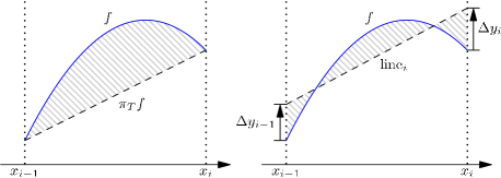
Let us now characterize the error of the orthogonal projection $P_{T}f$. We do so in two steps: first we compute the minimum error of a line segment in the interval $I_{i}$, and then we use an asymptotic analysis to approximate the error of the orthogonal projection.

Stemming from $\eqref{eq:LinearInterpolantInInterval}$, we can write any (linear) segment in $I_{i}$ as

$$\mathrm{line}_{i}(x)= \;\bigl{(}f(x_{i-1})+\Delta y_{i-1}\bigr{)}\bigl{(}1-\delta_{i}(x)\bigr{)}$$

$$+\bigl{(}f(x_{i})+\Delta y_{i}\bigr{)}\delta_{i}(x),$$ (10)

where $\Delta y_{i-1}$ and $\Delta y_{i}$ are extra degrees of freedom (pictured in Figure 4) with respect the interpolant $\pi_{T}f$ that allow the line segment to better approximate the function $f$ in $I_{i}$. By computing the optimal values of $\Delta y_{i-1}$ and $\Delta y_{i}$ we obtain the following result.

Result 2.

The minimum squared $L_{2}$ error between a given function $f$ and a line segment (10) in an interval $I_{i}=[x_{i-1},x_{i}]$, of length $h_{i}=x_{i}-x_{i-1}$, adopts the expression

$$\min\|f-\mathrm{line}_{i}\|_{L_{2}(I_{i})}^{2}=\frac{h_{i}^{5}}{120}(f^{\prime\prime}(\eta))^{2}$$

$$\quad-\frac{h_{i}^{5}}{144}\left(\bigl{(}f^{\prime\prime}(\eta_{0})\bigr{)}^{2}+\bigl{(}f^{\prime\prime}(\eta_{1})\bigr{)}^{2}-f^{\prime\prime}(\eta_{0})f^{\prime\prime}(\eta_{1})\right).$$ (11)

for some $\eta,\eta_{0},\eta_{1}$ in $(x_{i-1},x_{i})$.

Proof:

See Appendix B.

Corollary 2.1.

If $I_{i}$ is sufficiently small so that $f^{\prime\prime}$ is approximately constant within it, say $f^{\prime\prime}_{I_{i}}$, then

$$\min\|f-\mathrm{line}_{i}\|_{L_{2}(I_{i})}^{2}\approx\frac{h_{i}^{5}}{720}(f^{\prime\prime}_{I_{i}})^{2}.$$ (12)

Proof:

Substitute $f^{\prime\prime}(x)\approx f^{\prime\prime}_{I_{i}}$ for $x=\{\eta,\eta_{0},\eta_{1}\}$ in (11).

The segments in $P_{T}f$ may not strictly satisfy (11) because $P_{T}f$ must also be continuous across segments. However, as the size of the intervals $h_{i}$ become smaller (due to a finer partition $T$ of the interval $I$, i.e., the number of segments $N$ in $T$ increases) we may approximate $P_{T}f$ in $I_{i}$ by the best (independently-optimized) segment $\mathrm{line}_{i}$ and, consequently, use Corollary 2.1 to yield the following result.

Result 3.

The squared $L_{2}$ error between a given function $f$ and its orthogonal projection $P_{T}f$ in a small interval $I_{i}=[x_{i-1},x_{i}]$, of length $h_{i}=x_{i}-x_{i-1}$, is

$$\|f-P_{T}f\|_{L_{2}(I_{i})}^{2}\approx\frac{h_{i}^{5}}{720}(f^{\prime\prime}_{I_{i}})^{2}.$$ (13)

where $f^{\prime\prime}_{I_{i}}$ is the approximately constant value that $f^{\prime\prime}$ takes within the interval $I_{i}$.

Proof:

See Appendix C.

In the same asymptotic situation, the linear interpolant (9), (see (29)) gives a bigger squared error by a factor of six,

$$\|f-\pi_{T}f\|_{L_{2}(I_{i})}^{2}\approx\frac{h_{i}^{5}}{120}(f^{\prime\prime}_{I_{i}})^{2}.$$ (14)

III-B Approximation to the Optimal Partition

Now we give a procedure to compute a suboptimal partition of the target interval $I$ and then derive error estimates for both $\pi_{T}f$ and $P_{T}$ on such a partition and the uniform one.

III-B1 Procedure to Obtain a Suboptimal Partition

Let us consider a partition $T$ of $I=[a,b]$ with subintervals $I_{i}=[x_{i-1},x_{i}],\,i=1,\ldots,N$. A suboptimal partition for a given $N$ is one in which every subinterval has approximately equal contribution to the total approximation error [39, 40], which implies that regions of $f$ with higher convexity are approximated using more segments than regions with lower convexity. Let us assume $N$ is large enough so that $f^{\prime\prime}$ is approximately constant in each subinterval and therefore the bound (9) is tight. Consequently,

$$|f^{\prime\prime}_{i}|_{\max}h_{i}^{5/2}\approx C,$$ (15)

for some constant $C>0$, and the lengths of the subintervals (local knot spacing [40]) should be chosen $h_{i}\propto|f^{\prime\prime}_{i}|_{\max}^{-2/5}$, i.e., smaller intervals as $|f^{\prime\prime}_{i}|_{\max}$ increases. Hence, the local knot distribution or density is

$$lkd(x)\propto|f^{\prime\prime}(x)|^{2/5},$$ (16)

so that more knots of the partition are placed in the regions with larger magnitude of the second derivative.

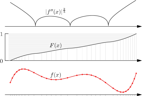
Then, the proposed approximation $T^{(\ast)}$ to the optimal partition is as follows: $x_{0}=a$, $x_{N}=b$, and take knots $\{x_{i}\}_{i=1}^{N-1}$ given by

$$F(x_{i})=i/N,$$ (17)

where the monotonically increasing function $F:[a,b]\to[0,1]$ is

$$F(x)=\int_{a}^{x}\bigl{(}f^{\prime\prime}(t)\bigr{)}^{2/5}\mathrm{d}t\Bigl{/}\int_{a}^{b}\bigl{(}f^{\prime\prime}(t)\bigr{)}^{2/5}\mathrm{d}t.$$ (18)

In this procedure, pictured in Figure 5, the range of $F(x)$ is divided into $N$ contiguous sub-ranges of equal length, and the values of $x_{i}$ are given by the abscissas corresponding to the endpoints of the sub-ranges.

III-B2 Error Estimates

With this partition, we can further estimate approximation error bounds in the entire interval based on those of the subintervals.

Result 4.

The approximation error of the linear interpolant $\pi_{T^{(\ast)}}f$ in the partition $T^{(\ast)}$ given by (17) in $I=[a,b]$ is

$$\|f-\pi_{T^{(\ast)}}f\|\lesssim\frac{1}{N^{2}\sqrt{120}}\left(\int_{a}^{b}\bigl{(}f^{\prime\prime}(t)\bigr{)}^{2/5}\mathrm{d}t\right)^{5/2}.$$ (19)

Proof:

The total squared error for any partition $T$ is the sum of squared errors over all subintervals $I_{i}$, and by (9),

$$\|f-\pi_{T}f\|^{2}\leq\sum_{i=1}^{N}\frac{1}{120}\left(|f^{\prime\prime}_{i}|_{\max}h_{i}^{5/2}\right)^{2},$$ (20)

which, under the condition of error equalization (15) for the proposed partition $T^{(\ast)}$, becomes

$$\|f-\pi_{T^{(\ast)}}f\|^{2}\leq\sum_{i=1}^{N}\frac{1}{120}C^{2}=\frac{1}{120}C^{2}N.$$ (21)

To compute $C$, let us sum $|f^{\prime\prime}_{i}|_{\max}^{2/5}h_{i}\approx C^{2/5}$ over all intervals $I_{i}$ and approximate the result using the Riemann integral:

$$C^{2/5}N\,\stackrel{{\scriptstyle\eqref{eq:ErrorEqualization}}}{{\approx}}\,\sum_{i=1}^{N}|f^{\prime\prime}_{i}|_{\max}^{2/5}h_{i}\approx\int_{a}^{b}\bigl{(}f^{\prime\prime}(t)\bigr{)}^{2/5}\mathrm{d}t,$$ (22)

whose right hand side is independent of $N$. Substituting (22) in (21) gives the desired approximate bound (19) for the error in the interval $I=[a,b]$.

Figure 5: Graphical summary of the proposed knot placement technique. Top: local knot density (16) obtained from input function $f$ (example in Figure 2); middle: cumulative knot distribution function $F$ given by (18) and knots given by the abscissas corresponding to a uniform partition of the range of $F$, as expressed by (17); bottom: approximation of $f$ by CPWL interpolant $\pi_{T^{\ast}}f$ with $N=31$ (32 knots). In this suboptimal partition, knots are distributed according to the amount of local convexity/concavity of $f$ given by the $lkd$ in the middle plot. Hence, fewer knots are placed around the zeros of the $lkd$, which correspond to the less steep regions of $F$.

Since the approximation error of $P_{T}f$ in each interval is roughly proportional to that of $\pi_{T}f$, as shown in (13) and (14), the partition (17) is also a very good approximation to the optimal partition for $P_{T}f$ as the number of subintervals $N$ increases. This is briefly stated next.

Result 5.

The approximation error of the orthogonal projection $P_{T^{(\ast)}}f$ in the partition $T^{(\ast)}$ given by (17) in $I=[a,b]$ is

$$\|f-P_{T^{(\ast)}}f\|\approx\frac{1}{\sqrt{6}}\|f-\pi_{T^{(\ast)}}f\|.$$ (23)

Both CPWL approximations ($\pi_{T}f$ and $P_{T}f$) converge to the true function $f$ at a rate of at least $O(N^{-2})$ ((19) and (23)).

We use a similar procedure to derive an estimate error bound for the uniform partition $T_{U}$ that can be compared to that of the optimized one.

Result 6.

The approximation error of the linear interpolant $\pi_{T_{U}}f$ in the uniform partition $T_{U}$ of the interval $I=[a,b]$ is

$$\|f-\pi_{T_{U}}f\|\approx\frac{\left(b-a\right)^{2}}{N^{2}\sqrt{120}}\|f^{\prime\prime}\|.$$ (24)

Proof:

For $T_{U}$, we may substitute $h_{i}=(b-a)/N$ in (20) and approximate the result using the Riemann integral,

$$\|f-\pi_{T_{U}}f\|\stackrel{{\scriptstyle\eqref{eq:SquaredBoundpipL2-prev}}}{{\leq}}\frac{h_{i}^{2}}{\sqrt{120}}\left(\sum_{i=1}^{N}|f^{\prime\prime}_{i}|_{\max}^{2}h_{i}\right)^{1/2}\approx\frac{\left(b-a\right)^{2}}{N^{2}\sqrt{120}}\|f^{\prime\prime}\|.$$

Thus, we can estimate how much we can expect to benefit from optimizing a partition by simply dividing (19) by (24). Since (24) also shows a $O(N^{-2})$ convergence, the profit will not depend on $N$ (assuming $N$ is large enough).

IV Computational Analysis

1     Determine the subinterval $I_{i}$ that contains $x^{\star}$: $i\mid x_{i-1}\leq x^{\star}<x_{i}$

2     Find the fractional distance $\delta_{i}$ to the left endpoint of $I_{i}$: $\delta_{i}\Leftarrow(x^{\star}-x_{i-1})/(x_{i}-x_{i-1})$

3     Return the interpolated value $\left(1-\delta_{i}\right)v(x_{i-1})+\delta_{i}\,v(x_{i})$

Algorithm 1 (CPWL function evaluation). Given as input the description of a continuous piecewise linear function (CPWL) $v\in\mathrm{V}_{T}$ by means of the the nodal values $\mathtt{v\_samples}=v(x_{0}),\ldots,v(x_{N})$ at the knots $\mathtt{x\_samples}=x_{0},\ldots,x_{N}$ of the partition $T$, and an abscissa $x^{\star}\in\left[x_{0},x_{N}\right)$, return $v(x^{\star})$.

The implementation of the approximations previously discussed is straightforward (Algorithm 1) and we only need to distinguish two different cases depending on whether the partition $T$ of $I$ has all subintervals of equal width or not. Although their values are different, $\pi_{T}f(x)$ and $P_{T}f(x)$ are qualitatively the same from the computational viewpoint.

Let us discuss the general case that $T$ is non-uniform. Line 1 in Algorithm 1 implies searching in the ordered array $\mathtt{x\_samples}$ for the right index $i$. Since the other steps in the algorithm do not depend on the size of the input vectors, Line 1 is the dominant step and makes its run-time complexity $O(\log N)$. In the particular case that $T$ is uniform, no search is needed to determine the index: $i\Leftarrow\bigl{\lfloor}\frac{x^{\star}-x_{0}}{x_{N}-x_{0}}N\bigr{\rfloor}+1$ and the fractional part $\delta_{i}\Leftarrow\frac{x^{\star}-x_{0}}{x_{N}-x_{0}}N+1-i$. Thus, the run-time complexity of the uniform case is $O(1)$. There is also no need to store the full array $\mathtt{x\_samples}$ but only its endpoints $x_{0}$ and $x_{N}$, roughly halving the memory needed for a non-uniform partition of the same number of intervals.

Consequently, approximations based on a uniform partition are expected to perform better in usual CPUs or GPUs, computationally-wise, than those based on non-uniform partitions. However, optimizing the partition might lead, depending on the specific objective function, to a reduction in the memory requirements for a desired approximation error. If memory constraints are relevant or hardware-aided search routines become available, optimized partitions could become practical.

V Implementation in a GPU

The proposed algorithm is simple to implement either in a CPU or in a GPU. However, there are some implementation details that help further optimize the performance in a GPU.

Modern GPUs implement a Single Instruction, Multiple Data (SIMD) execution model in which multiple threads execute exactly the same instructions (each) over different data. If two threads scheduled together in the same execution group or warp follow different branches in a conditional statement, both branches are not executed in parallel but sequentially, thereby halving throughput. In the case of $T$ being non-uniform, the (binary) search performed to find the index $i$ could lead to divergent paths for different threads evaluating $v(x)$ for different values of $x$, thus reducing throughput.

Since the purpose of the proposed algorithm is to save computation at run-time, it is reasonable to assume that at least $N$, and possibly $\mathtt{x\_samples}$ and $\mathtt{v\_samples}$ too, have been determined at compile time. Then, we can particularize the search code in compile time, unrolling the loop needed to implement the binary search and, most importantly, replacing conditional statements with a fixed number of invocations of the ternary operator, which is implemented in the GPU with a single instruction and no code divergence [41].

In general, accesses to memory in a GPU need to be arranged so that neighbouring threads access neighbouring addresses in memory. This allows the host interface of the GPU to coalesce operations from several threads into fewer transactions bigger in size. In the described algorithm, if each thread is evaluating $v(x)$ for different values of $x$, it is not guaranteed that the memory access pattern complies with this restriction. Although some devices provide caching and isolate the programmer from this issue, not all do.

However, there is a case in a regular computer graphics pipeline in which a similar problem arises. Texture data need to be accessed many times in a short period and it is generally impossible to ensure that neighbouring pixels in screen need to read neighbouring texels. Consequently, most GPUs do cache texture data and even have dedicated cache layers for it. We therefore store the arrays of samples in texture memory rather than in global memory to benefit from texture caches.

The use of the texture units to access our samples provides another important benefit. In the usual computer graphics pipeline, GPUs need to constantly filter texture data. In order to efficiently perform that task, texture units are equipped with hardware fixed-function interpolation routines that include linear interpolation [21]. Therefore, we can use them to speed up line 3 in Algorithm 1; results in the next section confirm that the texture filtering unit is indeed faster than performing interpolation “manually”.

VI Experimental Results

In this section we apply the proposed linearization algorithm to several functions of interest in cybernetics, computer vision and other scientific areas. The section starts with the analysis of the Gaussian function and demonstrates the proposed technique on an image processing application. The section then analyzes two other sample nonlinear functions of interest: the Lorentzian function and the Bessel function of the first kind.

VI-A Gaussian Function

The Gaussian function $f(x)=\exp(-x^{2}/2)/\sqrt{2\pi}$ is widely used in many applications in every field of science, but it is of particular interest to us in the context of foreground segmentation in video sequences using spatio-temporal nonparametric background models [20]. To estimate these models, the Gaussian function needs to be evaluated approximately 1300 times per pixel and input image, or around 2 billion times per second at modest video quality (CIF, $352\times 288$ pixels at 15 fps). Therefore it is crucial to lower the computing time of the Gaussian function. In the performed experiments it was enough to approximate the function in the interval $x\in\left[0,8\right]$ to achieve the required quality.

Figure 6: $L_{2}$ distance for different approximations to the Gaussian function $f(x)=\exp(-x^{2}/2)/\sqrt{2\pi}$ over the interval $x\in\left[0,8\right]$.

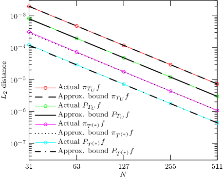
Figure 6 shows $L_{2}$ distances between the Gaussian function and the approximations described in previous sections. It reports actual distances as well as the approximate and tight upper bounds to the distances, i.e., Results 4 to 6. It can be observed that the $L_{2}$ distances between $\pi_{T}f$ and $f$ using the uniform and optimized partitions agree well with Results 4 to 6. All curves in Figure 6 have similar slope to that of (19), i.e., their convergence rate is $O(N^{-2})$, and the ratio between the distances corresponding to $P_{T}f$ and $\pi_{T}f$ is approximately the value $1/\sqrt{6}$ that stems from Result 3 and (14).

TABLE I: Mean per-evaluation execution times (in picoseconds) for the Gaussian function.

	Number of points ($N+1$)	32	64	128	256	512
CPU	exact function using expf from <cmath>	13710
	uniform partition	1750 - 1780
	optimized partition	8900	11230	13830	16910	20120
GPU	exact function using expf from <cmath>	33.3
	fast function using __expf from the SFU	14.2
	uniform partition, manual interpolation	19.7 - 19.8
	uniform partition, hardware interpolation	7.8 - 7.9
	optimized partition, manual interpolation	142.0	161.9	181.8	203.1	224.1
	optimized partition, hardware interpolation	122.7	142.9	163.2	188.3	211.1

Table I shows mean processing times per evaluation both in the CPU (sequentially, one core only) and in the GPU. All execution times have been measured in a computer equipped with an Intel Core i7-2600K processor, 16 GiB RAM and an NVIDIA GTX 580 GPU. We have exercised the utmost care to ensure that all different strategies achieve the same utilization of the GPU so that measurements are fair.

Figure 7: Mean per-evaluation execution times of all the proposed variants on a GPU (in picoseconds). The graph clearly shows the $O(1)$ and $O(\log N)$ dependencies on the number of intervals $N$ for uniform and non-uniform partitions, respectively.

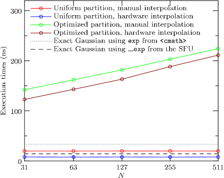
We compare the proposed algorithm against the exact Gaussian implemented using the exponential function of the C standard library (CPU or GPU) and against a fast Gaussian implemented using the hardware-accelerated low-precision exponential function from the SFU of the GPU [23]. In either hardware (CPU or GPU), there are no separate measurements for $\pi_{T}f(x)$ and $P_{T}f(x)$ because they only differ in value but not in their implementation. As was expected from the computational analysis, execution times for the uniform partition are constant, whereas they are heavily dependent on $N$ for the optimized partition (see Figure 7).

In the CPU case, the optimized partition approach is faster than the C standard library implementation if $N<128$, but the speed-up gain is smaller than that of the uniform partition approach, which is 8 times faster than the C standard library (regardless of $N$).

In the GPU case, we have also measured the proposed algorithm both with and without the texture filtering unit (last four rows of Table I) to prove that the former option is indeed faster than coding the interpolation explicitly, thanks to its dedicated circuitry. The proposed strategy, using a uniform partition (7.9 ps), solidly outperforms both the exact (33.3 ps) and fast SFU (14.2 ps) Gaussians, by approximate speed-up factors of $\times 4$ and $\times 2$, respectively, even though the latter is hardware-accelerated. However, we must stress that this is a synthetic benchmark; in a real application such as the one described in the next section, there may exist limitations in memory bandwidth to access operands. Moreover, many resources such as shared memory, cache and hardware registers are being used for other tasks too. This can (and does) affect the execution time of each of the different implementation strategies.

Foreground Segmentation (Sample Application)

(a)

(c)

(e)

(b)

(d)

(f)

Figure 8: Results from several different foreground segmentation methods for a complex dynamic scene. (a) Original scene; (b) Ground truth; (c) Temporal Median Filter; (d) Running Gaussian Average; (e) Mixture of Gaussians; (f) Nonparametric modeling.

To obtain high-quality detections in complex situations (e.g., dynamic background, illumination changes, etc.), multimodal moving object detection strategies are commonly used because they are able to model the multiple pixel states in such situations. Among multimodal strategies, nonparametric methods have shown to provide the best quality detections [42] because, in contrast to other algorithms, they do not assume that the pixel values conform to a particular distribution, but obtain instead probabilistic models from sets of recent samples.

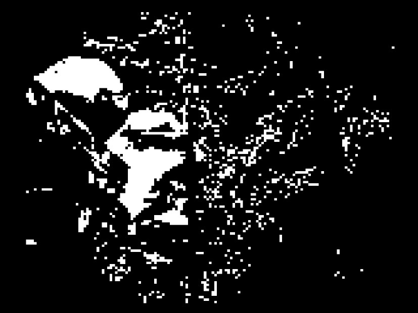
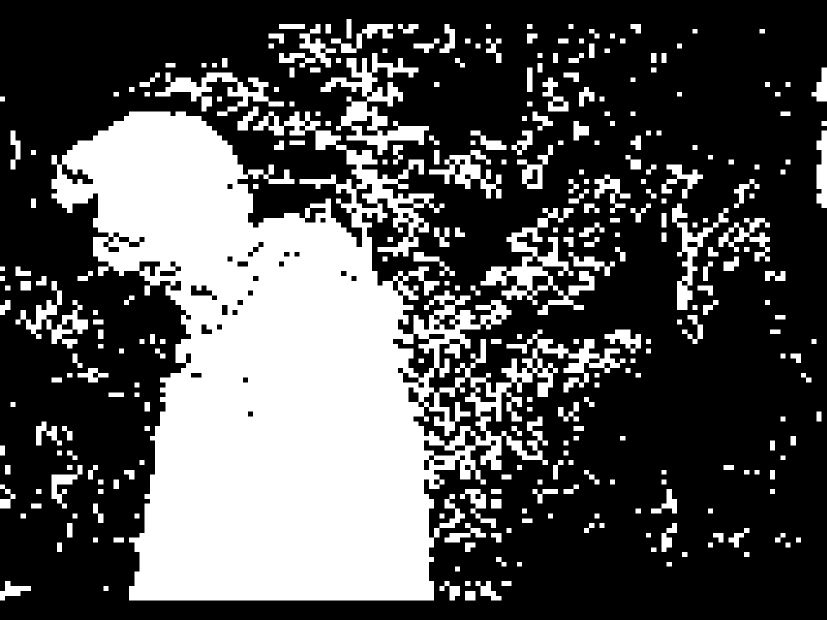
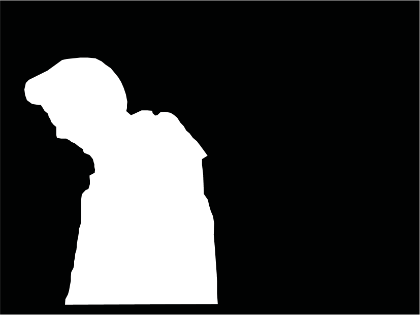
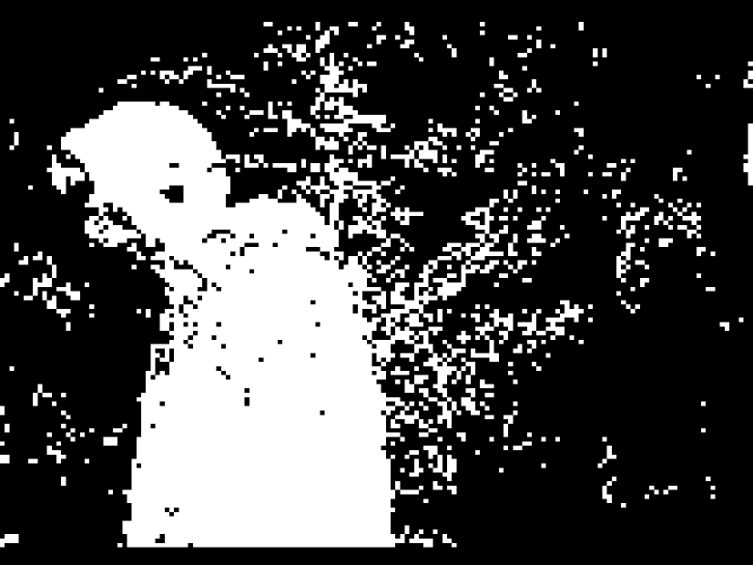
Figure 8 illustrates this by comparing the results from different strategies against a difficult scene featuring a dynamic background. The results of two unimodal background modeling methods are shown in the second row of this figure: the Temporal Median Filter (e.g., [43]) and the Running Gaussian Average (e.g., [44]); whereas the segmentations resulting from the application of two multimodal modeling approaches are depicted in the third row: an improved version of the Mixture of Gaussians method [45] and the spatio-temporal nonparametric-based background modeling in [20].

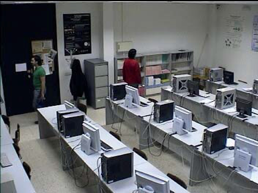
To improve the quality of the results in sequences containing non-static background regions, and/or captured with portable cameras, most recent nonparametric methods use spatio-temporal reference data [46]. However, these strategies involve huge memory and computational costs, since they need to evaluate millions of Gaussian kernels per image. Therefore, lowering the cost of evaluating the Gaussian function has a direct impact in the performance of the algorithm. To demonstrate this, we have implemented our proposed technique in a nonparametric background modeling method [20]. Table II shows mean per-pixel (in order to make measurements resolution-independent) processing times for the three best performing options in Section VI. Processing times are not proportional to those in Table I because the model needs to do many other things aside from evaluating Gaussians, and access to reference data is bandwidth-limited. However, our proposed technique still outperforms any of the alternatives: the exact Gaussian by 27% and the fast SFU Gaussian by 12%, while the final segmentation results of the method are the same in all three cases, as depicted in Figure 9.

TABLE II: Mean per-pixel processing times (in nanoseconds) for the nonparametric background modeling technique.

Uniform partition, hardware interpolation	286
Fast Gaussian using __expf from the SFU	324
Exact Gaussian using expf from <cmath>	391

(a)

(c)

(b)

(d)

Figure 9: Sample detections using nonparametric modeling with CPWL-approximated Gaussian kernels. Subfigures (a) and (b) show the original scene and results of the segmentation, respectively, for the tracking application; subfigures (c) and (d) show the original scene and results of the segmentation, respectively, for the video-based interface application.

VI-B Lorentzian Function

The performance of the approximation technique has also been tested on other functions. For example, the Lorentzian function with peak at $x_{0}$ and width $\gamma$ is

$$\mathcal{L}(x;x_{0},\gamma)=\frac{1}{\pi}\frac{\gamma}{(x-x_{0})^{2}+\gamma^{2}}$$ (25)

As a probability distribution, (25) is known as the Cauchy distribution. It is an important function in Physics since it solves the differential equation describing forced resonance. In such case, $x_{0}$ is the resonance frequency and $\gamma$ depends on the damping of the oscillator (and is inversely proportional to the $Q$ factor, a measure of the sharpness of the resonance).

Figure 10: $L_{2}$ distance for different CPWL approximations to the standard Cauchy distribution $f(x)=1/((1+x^{2})\pi)$ in the interval $x\in[0,6]$.

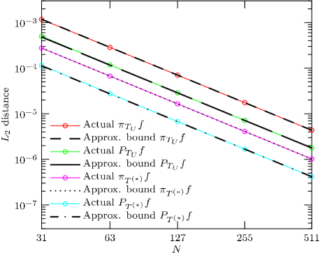
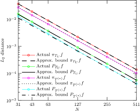
Figure 10 reports the $L_{2}$ distances between $\mathcal{L}(x;0,1)$ (25) and the CPWL approximations described in previous sections, in the interval $x\in[0,20]$. The measured errors agree well with the predicted approximate error bounds, showing the expected $O(N^{-2})$ trend.

We have measured the mean per-evaluation execution times of the exact function both in the CPU (576 ps) and in the GPU, both using regular and reduced-precision accelerated division (19.5 ps and 9.2 ps, respectively). The evaluation times of our proposed strategy coincide with those of the Gaussian function (Table I) because the processing time of the CPWL approximation does not depend on the function values.

As expected from the lower complexity of this function (compared to that of Sec. VI-A), which only involves elementary arithmetic operations, the advantage of our proposal vanishes in the CPU because the operations needed to manually perform interpolation, together with the two values that need to be fetched from memory, are actually more than what the direct evaluation requires. However, note that in the GPU our proposal still remains competitive due to these operations being carried out by the dedicated circuitry of the texture unit.

VI-C Bessel Function

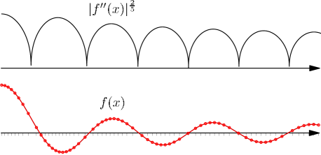
Approximating the Bessel function of the first kind $J_{0}(x)$ is more challenging than approximating the Gaussian or Lorentzian (bell-shaped) functions because it combines both nearly flat and oscillatory parts (see Figure 11). Figure 12 presents the $L_{2}$ approximation errors for $J_{0}(x)$ using CPWL functions in the interval $x\in[0,20]$. For $N\geq 63$ the measured errors agree well with the predicted approximate error bounds, whereas for $N<63$ the measured errors slightly differ from the predicted ones (specifically in the optimized partition) because in these cases the scarce number of linear segments does not properly represent the oscillations.

A sample optimized partition and the corresponding CPWL interpolant $\pi_{T^{\ast}}f$ is also represented in Figure 11. The knots of the partition are distributed according to the local knot density (see Figure 11, Top), accumulating in the regions of high oscillations (excluding the places around the zeros of the $lkd$).

This function is more complex to evaluate in general because it does not have a closed form. However, our approximation algorithm works equally well on it. We have measured the mean per-evaluation execution times in the CPU (39 ns using the POSIX extensions of the GNU C Library and 130 ns—only double-precision provided—using the GNU Scientific Library) and in the GPU (78 ps using the CUDA [23] standard library). We have also measured the execution time of the first term in the asymptotic expansion [47, Eq. 9.57a], valid for $x\gg 1/4$, $J_{0}(x)=\sqrt{\frac{2}{\pi x}}\left[\cos\left(x-\frac{\pi}{4}\right)+O\left(\frac{1}{x}\right)\right].$ In the GPU the evaluation takes 42 ps using reduced-precision accelerated functions from the SFU for the cosine and multiplicative inverse of the square root. Despite this approximation having a non-customizable error (decreasing as $x$ increases) and using the fastest available implementation (SFU) of the operations involved, our strategy still outperforms it by a sizable margin. This clearly illustrates that the more complex the function to be evaluated is, the greater the advantage of our proposal.

Figure 11: Suboptimal partition for the Bessel function $f(x)=J_{0}(x)$ in the interval $x\in[0,20]$. Top: local knot density ($lkd$) corresponding to $f$; bottom: CPWL interpolant $\pi_{T^{\ast}}f$ with $N=63$ ($64$ knots) overlaid on function $f$.

Figure 12: $L_{2}$ distance for different CPWL approximations to the Bessel function of the first kind $f(x)=J_{0}(x)$ in the interval $x\in[0,20]$.

VII Conclusions

We have developed a fast method to numerically evaluate any continuous mathematical function in a given interval using simpler continuous piecewise linear (CPWL) functions and the built-in routines present in the texture units of modern GPUs. Our technique allows real-time implementation of demanding computer vision and cybernetics applications that use such mathematical functions.

For this purpose, we analyzed the CPWL approximations given by the linear interpolant and the $L_{2}$ orthogonal projection of a function. We carried out a detailed error analysis in the $L_{2}$ distance to seek a nearly optimal design of both approximations. In the practical asymptotic case of a large number of subintervals $N$, we used error equalization to achieve a suboptimal design (partition $T^{\ast}$) and derived a tight bound on the approximation error for the linear interpolant, showing a $O(N^{-2})$ convergence rate that was confirmed by experimental results. The $L_{2}$ orthogonal projection can only but improve upon the results of the linear interpolant, resulting in a gain factor of $\sqrt{6}$.

We discussed the computational complexity and the implementation in a GPU of the numerical evaluation of both CPWL approximations. Our experimental results show that our technique can outperform both the quality and the computational cost of previous similar approaches. In particular, the fastest strategy consists of using the texture units in the GPU to evaluate either of the CPWL approximations defined over a uniform partition. This is normally faster than performing exact function evaluations, even when using the reduced-precision accelerated implementation of the SFUs in a GPU, or evaluating the proposed linear approximations without the assistance of the texture units. In practice, the number of subintervals $N$ to be considered for representing the nonlinear function can be decided on its own or based on other considerations such as a target approximation error, speed or memory constraints.

Although mathematically sound, the strategies based on a suboptimal (non-uniform) partition are not practical to implement in current CPU/GPU architectures due to the high cost incurred to find the subinterval that contains the given point of evaluation. Nevertheless, this opens future research paths to explore practical implementations of such approaches using specialized hardware.

Appendix A Proof of Result 1 (Linear Interpolant Error)

Recall one of the theorems on interpolation errors [48]. Let $f$ be a function in $C^{n+1}[a,b]$, and let $p$ be a polynomial of degree $n$ or less that interpolates the function $f$ at $n+1$ distinct points $x_{0},x_{1},\ldots,x_{n}\in[a,b]$. Then, for each $x\in[a,b]$ there exists a point $\xi_{x}\in[a,b]$ for which

$$f(x)-p(x)=\frac{1}{(n+1)!}f^{(n+1)}(\xi_{x})\prod_{k=0}^{n}(x-x_{k}).$$ (26)

In the interval $I_{i}$, the linear interpolant $\pi_{T}f$ is given by (8). Since $\pi_{T}f$ interpolates the function $f$ at the endpoints of $I_{i}$, we can apply theorem (26) (with $n=1$); hence, the approximation error solely depends on $f^{\prime\prime}$ and $x$, but not on $f$ or $f^{\prime}$:

$$f(x)-\pi_{T}f(x)=-\frac{1}{2}f^{\prime\prime}(\xi_{x})(x-x_{i-1})(x_{i}-x).$$ (27)

Let us integrate the square of (27) over the interval $I_{i}$,

$$\|f-\pi_{T}f\|_{L_{2}(I_{i})}^{2}=\int_{I_{i}}\frac{\bigl{(}f^{\prime\prime}(\xi_{x})\bigr{)}^{2}}{4}\bigl{(}(x-x_{i-1})(x_{i}-x)\bigr{)}^{2}\,\mathrm{d}x.$$

Next, to simplify the previous integral, let us use the first mean value theorem for integration, which states that if $u:[A,B]\rightarrow\mathbb{R}$ is a continuous function and $v$ is an integrable function that does not change sign on the interval $(A,B)$, then there exists a number $\eta\in(A,B)$ such that

$$\int_{A}^{B}u(x)v(x)\,\mathrm{d}x=u(\eta)\int_{A}^{B}v(x)\,\mathrm{d}x.$$ (28)

Since $(x-x_{i-1})\geq 0$ and $(x_{i}-x)\geq 0$ for all $x\in I_{i}$, let us apply (28) to compute

$$\|f-\pi_{T}f\|_{L_{2}(I_{i})}^{2} =\frac{1}{4}\bigl{(}f^{\prime\prime}(\eta)\bigr{)}^{2}\int_{I_{i}}\bigl{(}(x-x_{i-1})(x_{i}-x)\bigr{)}^{2}\,\mathrm{d}x$$

$$=\frac{h_{i}^{5}}{120}\bigl{(}f^{\prime\prime}(\eta)\bigr{)}^{2},$$ (29)

for some $\eta\in(x_{i-1},x_{i})$. Finally, if $|f^{\prime\prime}_{i}|_{\max}=\max_{\eta\in I_{i}}|f^{\prime\prime}(\eta)|$, it is straightforward to derive the $L_{2}$ error bound (9) from the square root of (29).

Appendix B Proof of Result 2 (Line Segment Minimum Error)

The approximation error corresponding to the line segment (10) is

$$f(x)-\mathrm{line}_{i}(x)=f(x)-\pi_{T}f(x)-(\pi_{T}\Delta y)(x)$$ (30)

where, by analogy with the form $\eqref{eq:LinearInterpolantInInterval}$ of $\pi_{T}f,$ we defined $(\pi_{T}\Delta y)(x)=\Delta y_{i-1}\bigl{(}1-\delta_{i}(x)\bigr{)}+\Delta y_{i}\delta_{i}(x)$.

The proof proceeds by computing the optimal values of $\Delta y_{i-1}$ and $\Delta y_{i}$ that minimize the squared $L_{2}$ error over the interval $I_{i}$:

$$\|f-\mathrm{line}_{i}\|_{L_{2}(I_{i})}^{2} \stackrel{{\scriptstyle\eqref{eq:f_minus_line}}}{{=}}\|f-\pi_{T}f\|_{L_{2}(I_{i})}^{2}+\|\pi_{T}\Delta y\|_{L_{2}(I_{i})}^{2}$$

$$\quad-2\left\langle f-\pi_{T}f,\pi_{T}\Delta y\right\rangle_{L_{2}(I_{i})}.$$ (31)

The first term is given in (29). The second term is

$$\|\pi_{T}\Delta y\|_{L_{2}(I_{i})}^{2}=\frac{h_{i}}{3}\left((\Delta y_{i-1})^{2}+(\Delta y_{i})^{2}+\Delta y_{i-1}\Delta y_{i}\right),$$

and the third term is, applying (28) and the change of variables $t=\delta_{i}(x)$ to evaluate the resulting integrals,

$$-2\left\langle f-\pi_{T}f,\pi_{T}\Delta y\right\rangle_{L_{2}(I_{i})}$$

$$=\Delta y_{i-1}\int_{I_{i}}f^{\prime\prime}(\xi_{x})(x-x_{i-1})(x_{i}-x)\bigl{(}1-\delta_{i}(x)\bigr{)}\,\mathrm{d}x$$

$$\quad+\Delta y_{i}\int_{I_{i}}f^{\prime\prime}(\xi_{x})(x-x_{i-1})(x_{i}-x)\delta_{i}(x)\,\mathrm{d}x$$

$$=\frac{h_{i}^{3}}{12}\bigl{(}\Delta y_{i-1}f^{\prime\prime}(\eta_{0})+\Delta y_{i}f^{\prime\prime}(\eta_{1})\bigr{)},$$

for some $\eta_{0}$ and $\eta_{1}$ in $(x_{i-1},x_{i})$.

Substituting previous results in (31),

$$\|f-\mathrm{line}_{i}\|_{L_{2}(I_{i})}^{2} =\frac{h_{i}}{3}\Bigl{(}(\Delta y_{i-1})^{2}+(\Delta y_{i})^{2}+\Delta y_{i-1}\Delta y_{i}\Bigr{)}$$

$$\quad+\frac{h_{i}^{3}}{12}\bigl{(}\Delta y_{i-1}f^{\prime\prime}(\eta_{0})+\Delta y_{i}f^{\prime\prime}(\eta_{1})\bigr{)}$$

$$\quad+\frac{h_{i}^{5}}{120}\bigl{(}f^{\prime\prime}(\eta)\bigr{)}^{2}.$$

We may now find the line segment that minimizes the distance to $f$ by taking partial derivatives with respect to $\Delta y_{i-1}$ and $\Delta y_{i}$, setting them to zero and solving the corresponding system of equations. Indeed, the previous error is quadratic in $\Delta y_{i-1}$ and $\Delta y_{i}$, and attains its minimum at

$$\begin{cases}\Delta y_{i-1}&=\bigl{(}f^{\prime\prime}(\eta_{1})-2f^{\prime\prime}(\eta_{0})\bigr{)}h_{i}^{2}/12,\\ \quad\Delta y_{i}&=\bigl{(}f^{\prime\prime}(\eta_{0})-2f^{\prime\prime}(\eta_{1})\bigr{)}h_{i}^{2}/12.\end{cases}$$ (32)

The resulting minimum squared distance is (11).

Appendix C Proof of Result 3 (Asymptotic Analysis)

By the triangle inequality, the jump discontinuity at $x=x_{i}$ between two adjacent independently-optimized segments is

$$\left|\Delta y_{i}^{-}-\Delta y_{i}^{+}\right| \leq\frac{h_{i}^{2}}{12}\,\bigl{|}f^{\prime\prime}(\eta_{0,i})-2f^{\prime\prime}(\eta_{1,i})\bigr{|}$$

$$\quad\;+\frac{h_{i+1}^{2}}{12}\,\bigl{|}f^{\prime\prime}(\eta_{1,i+1})-2f^{\prime\prime}(\eta_{0,i+1})\bigr{|},$$ (33)

where $\Delta y_{i}^{-}=\bigl{(}f^{\prime\prime}(\eta_{0,i})-2f^{\prime\prime}(\eta_{1,i})\bigr{)}h_{i}^{2}/12$ and $\Delta y_{i}^{+}=\bigl{(}f^{\prime\prime}(\eta_{1,i+1})-2f^{\prime\prime}(\eta_{0,i+1})\bigr{)}h_{i+1}^{2}/12$ are the offsets with respect to $f(x_{i})$ of the optimized segments (32) at the left and right of $x=x_{i}$, respectively; $\eta_{0,j}$ and $\eta_{1,j}$ lie in the interval $I_{j}$. Since we are dealing with functions twice continuously differentiable in a closed interval, the absolute value terms in (33) are bounded, according to the extreme value theorem; therefore, if $h_{i}$ and $h_{i+1}$ decrease (finer partition $T$), the discontinuity jumps at the knots of the partition also decrease. In the limit, as $\sup h_{i}\rightarrow 0$, $|\Delta y_{i}^{-}-\Delta y_{i}^{+}|\rightarrow 0$, i.e., continuity is satisfied. Therefore the union of the independently-optimized segments $\mathrm{line}_{i}\rightarrow P_{T}f$, which is the unique piecewise linear function satisfying both continuity ($\in\mathrm{V}_{T}$) and minimization of the $L_{2}$ error (7). Consequently, if $N$ is large we may approximate $\|f-P_{T}f\|_{L_{2}(I_{i})}^{2}\approx\min\|f-\mathrm{line}_{i}\|_{L_{2}(I_{i})}^{2}$; moreover, if $I_{i}$ is sufficiently small so that $f^{\prime\prime}$ is approximately constant within it, $f^{\prime\prime}_{I_{i}}$, then we use Corollary 2.1 to get (13).

References

- [1] G. Shapiro, “Consumer Electronics Association’s Five Technology Trends to Watch: Exploring New Tech That Will Impact Our Lives,” IEEE Consum. Electron. Mag., vol. 2, no. 1, pp. 32–35, 2013.
- [2] N. Singhal, I. K. Park, and S. Cho, “Implementation and optimization of image processing algorithms on handheld GPU,” in IEEE Int. Conf. Image Process. (ICIP), 2010, pp. 4481–4484.
- [3] V. Borges, M. Batista, and C. Barcelos, “A soft unsupervised two-phase image segmentation model based on global probability density functions,” in IEEE Int. Conf. Systems, Man and Cybernetics (SMC), Oct 2011, pp. 1687–1692.
- [4] K. Kapinchev, F. Barnes, A. Bradu, and A. Podoleanu, “Approaches to General Purpose GPU Acceleration of Digital Signal Processing in Optical Coherence Tomography Systems,” in IEEE Int. Conf. Systems, Man and Cybernetics (SMC), Oct 2013, pp. 2576–2580.
- [5] M. Song, D. Tao, Z. Liu, X. Li, and M. Zhou, “Image ratio features for facial expression recognition application,” IEEE Trans. Syst., Man, Cybern. B, vol. 40, no. 3, pp. 779–788, June 2010.
- [6] J. Kim, E. Park, X. Cui, H. Kim, and W. Gruver, “A fast feature extraction in object recognition using parallel processing on CPU and GPU,” in IEEE Int. Conf. Systems, Man and Cybernetics (SMC), Oct 2009, pp. 3842–3847.
- [7] S. Herrero-Lopez, “Accelerating SVMs by integrating GPUs into MapReduce clusters,” in IEEE Int. Conf. Systems, Man and Cybernetics (SMC), Oct 2011, pp. 1298–1305.
- [8] P. Kromer, J. Platos, and V. Snasel, “Genetic algorithm for clustering accelerated by the CUDA platform,” in IEEE Int. Conf. Systems, Man and Cybernetics (SMC), Oct 2012, pp. 1005–1010.
- [9] S. Balla-Arabe, X. Gao, and B. Wang, “GPU accelerated edge-region based level set evolution constrained by 2D gray-scale histogram,” IEEE Trans. Image Process., vol. 22, no. 7, pp. 2688–2698, 2013.
- [10] A. Jalba and J. B. T. M. Roerdink, “Efficient Surface Reconstruction From Noisy Data Using Regularized Membrane Potentials,” IEEE Trans. Image Process., vol. 18, no. 5, pp. 1119–1134, 2009.
- [11] S. Balla-Arabe, X. Gao, B. Wang, F. Yang, and V. Brost, “Multi-kernel implicit curve evolution for selected texture region segmentation in VHR satellite images,” IEEE Trans. Geosci. Remote Sens., vol. 52, no. 8, pp. 5183–5192, Aug 2014.
- [12] L. Cheng, M. Gong, D. Schuurmans, and T. Caelli, “Real-Time Discriminative Background Subtraction,” IEEE Trans. Image Process., vol. 20, no. 5, pp. 1401–1414, 2011.
- [13] P. Chiranjeevi and S. Sengupta, “Robust detection of moving objects in video sequences through rough set theory framework,” Image Vision Comput., vol. 30, no. 11, pp. 829 – 842, 2012.
- [14] N. Liu, H. Wu, and L. Lin, “Hierarchical ensemble of background models for PTZ-based video surveillance,” IEEE Trans. Cybern., vol. 45, no. 1, pp. 89–102, Jan 2015.
- [15] Y. Sheikh, O. Javed, and T. Kanade, “Background subtraction for freely moving cameras,” in IEEE Int. Conf. Computer Vision (ICCV). IEEE, 2009, pp. 1219–1225.
- [16] L. Sigal, M. Isard, H. Haussecker, and M. Black, “Loose-limbed people: Estimating 3D human pose and motion using non-parametric belief propagation,” Int. J. Comput. Vision, vol. 98, no. 1, pp. 15–48, 2012.
- [17] C. Cuevas, R. Mohedano, and N. García, “Adaptable Bayesian classifier for spatiotemporal nonparametric moving object detection strategies.” Optics letters, vol. 37, no. 15, pp. 3159–3161, Aug. 2012.
- [18] Y. Moshe, H. Hel-Or, and Y. Hel-Or, “Foreground detection using spatiotemporal projection kernels,” in IEEE Conf. Computer Vision and Pattern Recognition (CVPR), 2012, pp. 3210–3217.
- [19] C. Cuevas and N. García, “Efficient Moving Object Detection for Lightweight Applications on Smart Cameras,” IEEE Trans. Circuits Syst. Video Technol., vol. 23, no. 1, pp. 1–14, Jan. 2013.
- [20] D. Berjón, C. Cuevas, F. Morán, and N. García, “GPU-based implementation of an optimized nonparametric background modeling for real-time moving object detection,” IEEE Trans. Consum. Electron., vol. 59, no. 2, pp. 361–369, May 2013.
- [21] E. Lindholm, J. Nickolls, S. Oberman, and J. Montrym, “NVIDIA Tesla: A unified graphics and computing architecture,” IEEE Micro, vol. 28, no. 2, pp. 39–55, 2008.
- [22] M. Sylwestrzak, D. Szlag, M. Szkulmowski, I. Gorczyńska, D. Bukowska, M. Wojtkowski, and P. Targowski, “Real time 3D structural and Doppler OCT imaging on graphics processing units,” in Proc. SPIE, no. 85710Y. Int. Soc. Optics and Photonics, Mar. 2013.
- [23] NVIDIA Corp., “CUDA C Programming Guide,” Tech. Rep., 2012.
- [24] J. Gallego, M. Pardas, and J.-L. Landabaso, “Segmentation and tracking of static and moving objects in video surveillance scenarios,” in IEEE Int. Conf. Image Process. (ICIP), 2008, pp. 2716–2719.
- [25] M. Guillaumin, T. Mensink, J. Verbeek, and C. Schmid, “Face recognition from caption-based supervision,” Int. J. Comput. Vision, vol. 96, no. 1, pp. 64–82, 2012.
- [26] Z. Xie and L. Guan, “Multimodal Information Fusion of Audio Emotion Recognition Based on Kernel Entropy Component Analysis,” in IEEE Int. Symp. Multimedia, Dec. 2012, pp. 1–8.
- [27] M. Sehili, D. Istrate, B. Dorizzi, and J. Boudy, “Daily sound recognition using a combination of GMM and SVM for home automation,” in Proc. 20th European Signal Process. Conf., Bucharest, 2012, pp. 1673–1677.
- [28] M. Storace and O. De Feo, “Piecewise-linear approximation of nonlinear dynamical systems,” IEEE Trans. Circuits Syst. I, vol. 51, no. 4, pp. 830–842, 2004.
- [29] T. Hatanaka, K. Uosaki, and M. Koga, “Evolutionary computation approach to Wiener model identification,” in Congr. Evolutionary Computation (CEC ’02), vol. 1, 2002, pp. 914–919.
- [30] R. Tanjad and S. Wongsa, “Model structure selection strategy for Wiener model identification with piecewise linearisation,” in Int. Conf. Elect. Eng./Electron., Comput., Telecommun. and Inform. Technol. (ECTI-CON), 2011, pp. 553–556.
- [31] R. Rossi, S. A. Tarim, S. Prestwich, and B. Hnich, “Piecewise linear approximations of the standard normal first order loss function,” arXiv:1307.1708 [math.OC], 2013.
- [32] P. Julian, A. Desages, and O. Agamennoni, “High-level canonical piecewise linear representation using a simplicial partition,” IEEE Trans. Circuits Syst. I, vol. 46, no. 4, pp. 463–480, 1999.
- [33] P. Julian, A. Desages, and B. D’Amico, “Orthonormal high-level canonical PWL functions with applications to model reduction,” IEEE Trans. Circuits Syst. I, vol. 47, no. 5, pp. 702–712, 2000.
- [34] R. Bellman and R. Roth, “Curve fitting by segmented straight lines,” J. Amer. Statistical Assoc., vol. 64, no. 327, pp. 1079–1084, 1969.
- [35] C. Frenzen, T. Sasao, and J. Butler, “On the number of segments needed in a piecewise linear approximation,” J. Comput. and Appl. Math., vol. 234, no. 2, pp. 437–446, 2010.
- [36] S. Ghosh, A. Ray, D. Yadav, and B. M. Karan, “A Genetic Algorithm Based Clustering Approach for Piecewise Linearization of Nonlinear Functions,” in Int. Conf. Devices and Communications, 2011, pp. 1–4.
- [37] G. Gallego, D. Berjón, and N. García, “Optimal Polygonal Linearization and Fast Interpolation of Nonlinear Systems,” IEEE Trans. Circuits Syst. I, vol. 61, no. 11, pp. 3225–3234, Nov 2014.
- [38] K. Eriksson, D. Estep, and C. Johnson, “Piecewise linear approximation,” in Applied Mathematics: Body and Soul. Springer, 2004, vol. 2, ch. 52, pp. 743–754.
- [39] C. de Boor, “Piecewise linear approximation,” in A Practical Guide to Splines. Springer, 2001, ch. 3, pp. 31–37.
- [40] M. Cox, P. Harris, and P. Kenward, “Fixed- and free-knot univariate least-square data approximation by polynomial splines,” in 4th Int. Symp. Algorithms for Approximation, Jul. 2001, pp. 330–345.
- [41] V. K. Pallipuram, N. Raut, X. Ren, M. C. Smith, and S. Naik, “A Multi-Node GPGPU Implementation of Non-Linear Anisotropic Diffusion Filter,” in Symp. Application Accelerators in High Performance Computing, Jul. 2012, pp. 11–18.
- [42] C. Cuevas and N. García, “Improved background modeling for real-time spatio-temporal non-parametric moving object detection strategies,” Image Vision Comput., vol. 31, no. 9, pp. 616–630, 2013.
- [43] R. Cucchiara, C. Grana, M. Piccardi, and A. Prati, “Detecting moving objects, ghosts, and shadows in video streams,” IEEE Trans. Pattern Anal. Mach. Intell., vol. 25, no. 10, pp. 1337–1342, 2003.
- [44] Z. Tang, Z. Miao, and Y. Wan, “Background subtraction using running Gaussian average and frame difference,” in Int. Conf. Entertainment Computing (ICEC), 2007, pp. 411–414.
- [45] C. Cuevas, N. García, and L. Salgado, “A new strategy based on adaptive mixture of Gaussians for real-time moving objects segmentation,” in Proc. SPIE, no. 6811. Int. Soc. Optics and Photonics, 2008.
- [46] Y. Sheikh and M. Shah, “Bayesian modeling of dynamic scenes for object detection,” IEEE Trans. Pattern Anal. Mach. Intell., vol. 27, no. 11, pp. 1778–1792, 2005.
- [47] I. Bronshtein, K. Semendyayev, G. Musiol, and H. Mühlig, Handbook of Mathematics, 6th ed. Springer, 2015.
- [48] E. W. Cheney and D. R. Kincaid, “Errors in polynomial interpolation,” in Numerical Mathematics and Computing, 7th ed. Cengage Learning, 2012, ch. 4.2, p. 181.