Running head: Dissecting eQTL hotspots

Key words: eQTL, pleiotropy, multivariate analysis, data visualization, gene expression

¹Corresponding author:

Karl W Broman
Department of Biostatistics and Medical Informatics
University of Wisconsin–Madison
2126 Genetics-Biotechnology Center
425 Henry Mall
Madison, WI 53706
Phone:	608–262–4633
Email:	kbroman@biostat.wisc.edu

Abstract

Studies of the genetic loci that contribute to variation in gene expression frequently identify loci with broad effect on gene expression: expression quantitative trait locus (eQTL) hotspots. We describe a set of exploratory graphical methods as well as a formal likelihood-based test for assessing whether a given hotspot is due to one or multiple polymorphisms. We first look at the pattern of effects of the locus on the expression traits that map to the locus: the direction of the effects, as well as the degree of dominance. A second technique is to focus on the individuals that exhibit no recombination event in the region, apply dimensionality reduction (such as with linear discriminant analysis) and compare the phenotype distribution in the non-recombinants to that in the recombinant individuals: If the recombinant individuals display a different expression pattern than the non-recombinants, this indicates the presence of multiple causal polymorphisms. In the formal likelihood-based test, we compare a two-locus model, with each expression trait affected by one or the other locus, to a single-locus model. We apply our methods to a large mouse intercross with gene expression microarray data on six tissues.

Introduction

There is a long history of efforts to map the genetic loci (called quantitative trait loci, QTL) that contribute to variation in quantitative traits in experimental organisms, particularly to learn about the etiology of disease (Broman 2001; Jansen 2007). But it remains difficult to identify the genes underlying QTL (Nadeau and Frankel 2000). There has recently been much interest in measuring gene expression in disease-relevant tissues in QTL experiments, as a way to speed the process from QTL to gene (Jansen and Nap 2001; Albert and Kruglyak 2015). The genetic control of gene expression is itself of great interest.

Expression quantitative trait loci (eQTL) analysis tries to find the genomic locations that influence variation in gene expression levels (mRNA abundances). eQTL near the genomic location of the influenced gene are called local eQTL, and eQTL far away from the influenced gene are called trans-eQTL. When a genomic region influences the expression of many genes, the region is called a trans-eQTL hotspot.

eQTL hotspots have been observed in many genetic studies (e.g., Brem et al. 2002; Yvert et al. 2003; Schadt et al. 2003; Chesler et al. 2005), and they are of particular interest because gene expressions mapping to the same location may indicate the existence of a genetic regulator.

Batch effects (artifacts arising from technical or environmental factors) are common in microarray experiments. This has led to the development of a number of methods to control for underlying confounding factors (Leek and Storey 2007; Kang et al. 2008; Stegle et al. 2010; Listgarten et al. 2010; Gagnon-Bartsch and Speed 2012; Fusi et al. 2012). However, these methods generally cannot distinguish trans-eQTL hotspots from batch effects. There is some controversy about whether trans-eQTL hotspots are themselves artifacts and whether one should control for them, as one does for batch effects, in eQTL analysis (e.g., Breitling et al. 2008; Kang et al. 2008). But in many cases, the associations between genotype and expression phenotypes are extremely strong (with LOD $>$ 100), which largely precludes the possibility of a batch effect artifact, as the strength of association between batch and genotype in the region would have to be even stronger.

In Tian et al. (2015), we considered a large mouse intercross between the strains C57BL/6J (abbreviated B6) and BTBR $T^{+}$ tf/J (abbreviated BTBR), with gene expression microarray data on six tissues (adipose, gastrocnemius muscle, hypothalamus, pancreatic islets, kidney, and liver), and mapped a trans-eQTL hotspot to a 298 kb region containing just three genes. This sort of fine-mapping approach is meaningful only if the hotspot is due to polymorphisms in a single gene.

This raises an important question about trans-eQTL hotspots: are they the result of polymorphisms in a single gene, or are there multiple underlying genes? In other words, is there complete pleiotropy, or are there multiple linked eQTL? Methods for testing pleiotropy versus tight linkage of multiple QTL (Jiang and Zeng 1995; Knott and Haley 2000) do not scale well to the case of the very large number of expression traits that map to a trans-eQTL hotspot. We developed a likelihood-based test that is a variation on the method of Knott and Haley (2000), as well as a number of exploratory data visualizations, to test whether multiple eQTL underlie a hotspot. We apply our approaches to the data considered in Tian et al. (2015).

Methods

We focus on the case of an intercross between two inbred strains, B and R (these labels were chosen to match the strains used in the application, below). We assume dense marker genotype data and genome-wide gene expression phenotype data (such as from microarrays or RNA-sequencing). We first perform a genome scan to identify quantitative trait loci (QTL), considering each expression trait individually. We use Haley-Knott regression (Haley and Knott 1992) for this purpose, for the sake of speed. For each expression trait and each chromosome, we consider the location of the single-largest LOD score, provided that it exceeds a significance threshold that adjusts for the genome scan but not the search across expression traits.

We count the number of expression traits that show a trans-eQTL within a sliding window (e.g., of 10 cM) across the genome, and use peaks in these counts to define trans-eQTL hotspots. We then focus on one such hotspot, and on the set of expression traits that map to an interval centered at the peak count.

We then ask: Are the multiple expression traits that map to this trans-eQTL hotspot all affected by a common eQTL, or could there be multiple causal polymorphisms in the region? We have developed a set of exploratory data visualizations to address this question, as well as a formal likelihood-based test. We prefer to exclude expression traits whose genomic position is near (or even on the same chromosome as) the hotspot of interest, as these may be driven by separate, local-eQTL.

Exploratory data visualizations

We first consider the pattern of effects of the locus on the expression traits that map to the region: the direction of the effects, as well as the degree of dominance. We use a pair of data visualizations: first, a plot of the signed LOD score (with the sign taken from the estimated additive effect) versus the estimated eQTL location, for each expression trait analyzed separately. That is, for each expression trait, we find the largest LOD score on the chromosome, multiply it by $\pm$1, according to the sign of the estimated additive effect of the locus, and plot this signed LOD score versus the location at which that maximum LOD score was attained. If there are two nearby loci with effects in opposite directions, they may be revealed by this plot.

In addition, we plot the estimated dominance effect against the estimated additive effect, for each expression trait. Let B and R denote the two alleles in the cross, and let $\hat{\mu}_{\text{BB}}$, $\hat{\mu}_{\text{BR}}$ and $\hat{\mu}_{\text{RR}}$ denote the average expression levels for genotypes BB, BR, and RR, respectively. We estimate the additive effect as half the difference between the two homozygotes, $\hat{a}=(\hat{\mu}_{\text{RR}}-\hat{\mu}_{\text{BB}})/2$, and the dominance effect as the difference between the heterozygote and the midpoint between the two homozygotes, $\hat{d}=\hat{\mu}_{\text{BR}}-(\hat{\mu}_{\text{BB}}+\hat{\mu}_{\text{RR}})/2$. We then plot $\hat{d}$ vs $\hat{a}$ for all expression traits mapping to the hotspot. If there are two nearby loci with different inheritance patterns (e.g., one has additive allele effects and the other has an allele that is dominant), they may be revealed by this plot.

As a second technique, we consider the individuals that have no recombination event in the region. For these individuals, we know their eQTL genotype. We apply linear discriminant analysis (LDA, Hastie et al. 2009, Ch. 4) to the top 100 traits with the largest LOD scores and make a scatterplot of the first and second linear discriminants; this should show three distinct clusters (or, for a fully dominant locus, two clusters). We calculate the linear discriminants for individuals that show a recombination event in the region, and add them as points to the plot. If the recombinant individuals fall within the clusters defined by the non-recombinants, this is consistent with there being a single causal locus. If, on the other hand, the recombinants look distinctly different from the non-recombinants, then multiple polymorphisms are indicated.

The basic idea underlying this visualization is that the non-recombinants can be used to derive an estimate of the conditional distribution of the multivariate expression phenotype, given the eQTL genotype. We use LDA as a dimension-reduction technique. The goal of the visualization is to compare the expression pattern in the recombinants and non-recombinants. If there is a single eQTL, the recombinants should look no different from the non-recombinants; if there is a difference, we can conclude that there are multiple eQTL.

Formal statistical test

To formally assess evidence of multiple linked loci versus complete pleiotropy at a trans-eQTL hotspot, we developed a likelihood-based test to compare the null hypothesis of a single eQTL affecting all expression traits to the hypothesis of two eQTL, with each expression trait affected by one or the other eQTL (but not both). The approach can handle only a limited number of expression traits, and so we focus on the 50 traits with largest LOD scores (when considered individually) in the interval centered at the hotspot.

We assume that the traits follow a multivariate normal distribution, conditional on eQTL genotype, and apply the multivariate QTL analysis method of Knott and Haley (2000). For a given QTL model, we have $Y=X\beta+E$, where $Y$ is an $n\times p$ matrix of phenotypes, with $n$ as the number of F₂ individuals and $p$ as the number of traits, $X$ is an $n\times q$ matrix of covariates (including additive covariates, interactive covariates, genotype probabilities for the position under investigation, and the interactive covariates times the genotype probabilities), and $\beta$ is a $q\times p$ matrix of coefficients. We obtain $\hat{\beta}=(X^{\prime}X)^{-1}X^{\prime}Y$, calculate the matrix of estimated residuals $\hat{E}=Y-X\hat{\beta}$, and calculate the residual sum of squares matrix $\text{RSS}=\hat{E}^{\prime}\hat{E}$. The LOD score is $\frac{n}{2}\log_{10}\{|\text{RSS}_{0}|/|\text{RSS}|\}$, where $|\text{RSS}|$ denotes the determinant of the RSS matrix, and $\text{RSS}_{0}$ is the residual sum of squares matrix for the null model (with additive covariates, but no genotype probabilities or interactive covariates).

We perform a QTL scan over the interval; at each putative QTL location, denoted $\lambda$, we calculate the LOD score, $\text{LOD}_{1}(\lambda)$, comparing this single-QTL model to the null model of no QTL. Let $M_{1}=\max_{\lambda}\text{LOD}_{1}(\lambda)$.

We compare this to a two-QTL model, in which each expression trait is affected by one or the other QTL but not both. In principle, one would need to consider, with $p$ expression traits, $2^{p-1}$ possible assignments of the expression traits to the left and right QTL. This is a prohibitively large number, and so we make an approximation: we sort the expression traits according to their estimated QTL location, when considered individually, and we consider only the $p-1$ cut-points of this list. We randomly order any expression traits that map to the same position. For each cut-point, we perform a two-dimensional scan over possible two-QTL models, and calculate $\text{LOD}_{2}^{(c)}(\lambda_{1},\lambda_{2})$, comparing the two-QTL model, with QTL at positions $\lambda_{1}$ and $\lambda_{2}$ and with the first $c$ expression traits affected by the QTL at $\lambda_{1}$ and the last $p-c$ traits affected by the QTL at $\lambda_{2}$. Let $M_{2}^{(c)}=\max_{\lambda_{1},\lambda_{2}}\text{LOD}_{2}^{(c)}(\lambda_{1},\lambda_{2})$, and let $M_{2}=\max_{c}M_{2}^{(c)}$. The estimated cut-point is $\hat{c}=\arg\max_{c}M_{2}^{(c)}$, and the estimated QTL positions are $(\hat{\lambda}_{1},\hat{\lambda}_{2})=\arg\max_{\lambda_{1},\lambda_{2}}\text{LOD}_{2}^{(\hat{c})}(\lambda_{1},\lambda_{2})$.

As evidence for the presence of two QTL, we consider the log₁₀ likelihood ratio, $\text{LOD}_{2v1}=M_{2}-M_{1}$.

The exhaustive two-dimensional scan of $\text{LOD}_{2}^{(c)}(\lambda_{1},\lambda_{2})$ is computationally intensive. We can accelerate this calculation by iteratively searching for the maximum on each of the two dimensions. There is no guarantee that this will converge to the overall maximum, especially when there are multiple modes in the two-QTL likelihood surface, but in practice we’ve found this algorithm works well. As a starting point of this iterative search, we can use either the estimated QTL location under the single-QTL model, or a randomly selected position.

Statistical significance: To assess the statistical significance of the result, we need an approximation of the distribution of the test statistic under the null hypothesis of a single QTL. We consider two approaches: a parametric bootstrap, and a stratified permutation test.

In the parametric bootstrap, we simulate new phenotype data using the estimated single-QTL model. In the stratified permutation test, we randomly permute the rows in the phenotype data relative to the rows in the genotype data, within each QTL genotype group. When there are unmeasured genotypes at the inferred QTL, we infer the QTL genotype, for each individual, to be that with maximum probability, conditional on the observed marker data. These conditional QTL genotype probabilities are calculated by a hidden Markov model (Broman and Sen 2009, App. D).

For each procedure, we generate 1000 data sets, perform the full likelihood analysis (the scan for the single-QTL model, and the two-dimensional scan for the two-QTL model, for each possible partition of the traits) and calculate the test statistic. The P-value for the test is taken to be the proportion of simulated or permuted data sets with a test statistic that is greater or equal to the observed test statistic.

Visualizations: To visualize the results for the two-QTL model, we plot profile LOD curves for the left and right QTL, using the estimated cut-point, $\hat{c}$, for the expression traits into those mapping to the left QTL and those mapping to the right QTL. For the left QTL, we plot the slice $\text{LOD}_{2}^{(\hat{c})}(\lambda_{1},\hat{\lambda}_{2})$ against $\lambda_{1}$, for varying values of $\lambda_{1}$. Similarly, for the right QTL, we plot $\text{LOD}_{2}^{(\hat{c})}(\hat{\lambda}_{1},\lambda_{2})$ against $\lambda_{2}$, for varying values of $\lambda_{2}$. These sorts of profile LOD curves follow from an innovation of Zeng et al. (2000).

As a further diagnostic plot, we consider the statistic $\text{LOD}_{2v1}^{(c)}=M_{2}^{(c)}-M_{1}$, as a function of the cut-point, $c$. This is evidence for two vs one QTL, for a given cut-point, of the expression traits, into those that map to the left QTL and those that map to the right QTL. This displays the evidence for two vs one QTL as well as the evidence for a particular split of the expression traits.

Application

To illustrate our methods for the dissection of trans-eQTL hotspots, we consider a large mouse F₂ intercross (Tian et al. 2015) with gene expression microarray data on six tissues. The data are available at the QTL Archive, now part of the Mouse Phenome Database:
http://phenome.jax.org/db/q?rtn=projects/projdet&reqprojid=532

Materials

The experiment was carried out in order to identify genes and pathways that contribute to obesity-induced type II diabetes. Greater than 500 offspring were generated from an F₂ intercross between diabetes-resistant (C57BL/6J, abbreviated B6) and diabetes-susceptible (BTBR T⁺ tf/J, abbreviated BTBR) mouse strains. All mice were genetically obese through introgression of the leptin mutation (Lep^ob/ob) and were sacrificed at 10 weeks of age, the age when essentially all BTBR ob/ob mice are diabetic.

Mice were genotyped with the 5K GeneChip (Affymetrix). After data cleaning, there were 519 F₂ mice genotyped at 2,057 informative markers. Gene expression was assayed with custom two-color ink-jet microarrays manufactured by Agilent Technologies (Palo Alto, CA). Six tissues from each F₂ mouse were used for expression profiling: adipose, gastrocnemius muscle (abbreviated gastroc), hypothalamus (abbreviated hypo), pancreatic islets (abbreviated islet), kidney, and liver. Tissue-specific mRNA pools were used for the reference channel, and gene expression was quantified as the ratio of the mean log₁₀ intensity (mlratio). For further details, see Keller et al. (2008). In the final data set, there were 519 mice with gene expression data on at least one tissue (487 for adipose, 490 for gastroc, 369 for hypo, 491 for islet, 474 for kidney, and 483 for liver). The microarray included 40,572 total probes; we focused on the 37,797 probes with known location on one of the autosomes or the X chromosome.

QTL analysis

For QTL analysis, we first transformed the gene expression measures for each microarray probe in each of the six tissues to normal quantiles, taking $\Phi^{-1}[(R_{i}-0.5)/n]$, where $\Phi$ is the cumulative distribution function for the standard normal distribution and $R_{i}$ is the rank in $\{1,\dots,n\}$ for mouse $i$. We then performed single-QTL genome scans, separately for each probe in each tissue, by Haley-Knott regression (Haley and Knott 1992) with microarray batch as an additive covariate and with sex as an interactive covariate (i.e. allowing the effects of QTL to be different in the two sexes). Calculations were performed at the genetic markers and at a set of pseudomarkers inserted into marker intervals, selected so that adjacent positions were separated by $\leq$ 0.5 cM. We calculated conditional genotype probabilities, given observed multipoint marker genotype data, using a hidden Markov model assuming a genotyping error rate of 0.2%, and with genetic distances converted to recombination fractions with the Carter-Falconer map function (Carter and Falconer 1951). Calculations were performed with R/qtl (Broman et al. 2003), an add-on package to the general statistical software R (R Core Team 2015).

For each probe in each tissue, we focused on the single largest LOD score peak on each chromosome, and on LOD score peaks $\geq$ 5 (corresponding to genome-wide significance at the 5% level, for a single probe in a single tissue, determined by computer simulations under the null hypothesis of no QTL).

The inferred eQTL for all genes with LOD $\geq$ 5 are displayed in Figure 1, with the y-axis corresponding to the genomic position of the microarray probe and the x-axis corresponding to the estimated eQTL position. As expected, we see a large number of local-eQTL along the diagonal for each tissue-specific panel. These local-eQTL correspond to genes for which expression or mRNA abundance is strongly associated with genotype near their genomic position.

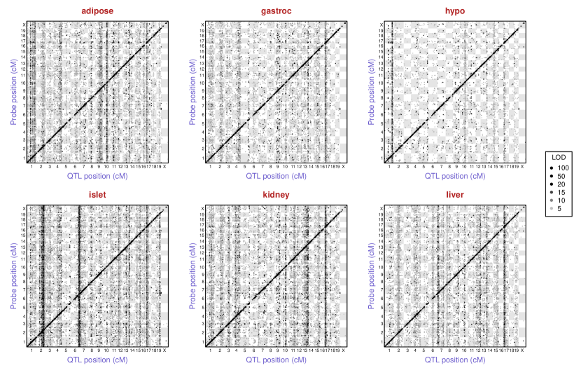
Figure 1: Inferred eQTL with LOD $\geq$ 5, by tissue. Points correspond to peak LOD scores from single-QTL genome scans with each microarray probe with known genomic position. The y-axis is the position of the probe and the x-axis is the inferred QTL position. Points are shaded according to the corresponding LOD score, though we threshold at 100: all points with LOD $\geq$ 100 are black. (A version of this figure appeared as Figure 1 in Tian et al. 2015)

In addition to the local-eQTL, there are a number of prominent vertical bands: genomic loci that influence the expression of genes located throughout the genome. These are the trans-eQTL hotspots. Overall, we detected many more trans-eQTL than local-eQTL. The trans-eQTL hotspots can show either remarkable tissue specificity or be observed in multiple tissues. For example, a locus near the centromere of chromosome 17, at 11.7 cM, shows effects in all tissues. In contrast, the trans-eQTL hotspot located at the distal end of chromosome 6 was only observed in pancreatic islets.

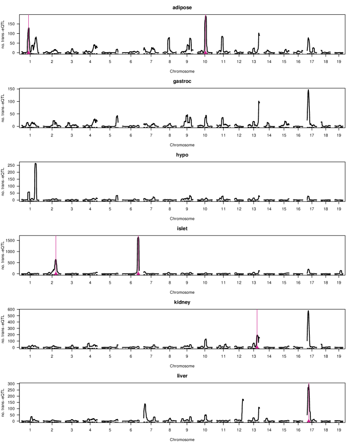
Figure S1: Number of expression traits with LOD $\geq$ 10 in a 10 cM sliding window across the genome. Red triangles indicate the six trans-eQTL hotspots used as examples in Figures 2, 3, and 5.

To define trans-eQTL hotspots of potential interest, we focused on a more conservative threshold for eQTL, of LOD $\geq$ 10. We further excluded local-eQTL, defined here to be those for which the distance between the gene’s genomic position and its inferred eQTL position was $<$ 10 cM. We then counted the number of expression traits with a trans-eQTL in a sliding interval of length 10 cM (Figure S1).

For each trans-eQTL of interest, we widened the interval to be considered beyond that initial 10 cM window, to consider the interval in which the count of expression traits with eQTL was $>$ 50, and then padded this further by adding 5 cM on either end.

We will focus on a set of six hotspots: adipose chromosome 1 at 39 cM, adipose chromosome 10 at 48 cM, islet chromosome 2 at 75 cM, islet chromosome 6 at 91 cM, kidney chromosome 13 at 68 cM, and liver chromosome 17 at 18 cM. Results for additional hotspots are displayed in File S1.

Visualization of QTL effects

We first consider the estimated effects of a locus on the expression traits that map to the region (Figure 2). In the left panels, we display the signed LOD score (with positive values indicating that the BTBR allele is associated with larger average expression and negative values indicating that the B6 allele is associated with larger average expression) versus the estimated eQTL location. In the right panels, we plot the estimated dominance effect versus the estimated additive effect for all transcripts mapping to the hotspot. The key value, in these visualizations, is for the case that two linked QTL show distinct inheritance patterns.

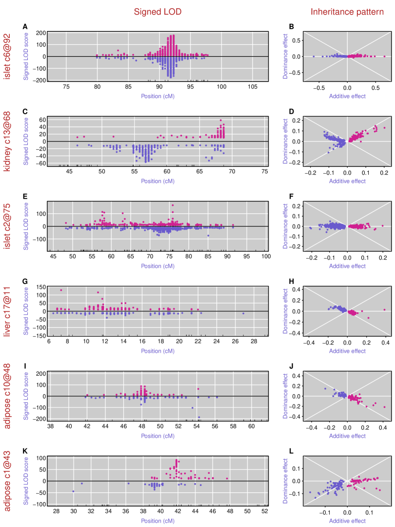
Figure 2: Visualizations of the QTL effects on the multiple expression traits that map with LOD $\geq$ 10 to a trans-eQTL hotspot. Each row is a hotspot. The left panels are scatterplots of signed LOD scores (with positive values indicating that the BTBR allele is associated with larger average gene expression and negative values indicating that the B6 allele is associated with larger average gene expression) versus the estimated QTL location. Each point is a single expression trait. Tick marks at the bottom indicate the locations of the genetic markers. The right panels are scatterplots of the estimated dominance effects versus the estimated additive effects.

The islet chromosome 6 hotspot, at 92 cM, shows approximately equal numbers of expression traits for which the BTBR allele causes an increase or decrease in gene expression (Figure 2A), and the allele effects are approximately additive (Figure 2B), with estimated dominance effect near 0. These results are consistent with there being a single QTL. In Tian et al. (2015), this locus was resolved to a 298 kb interval containing just three genes, with good evidence for Slco1a6 as the causal gene.

The kidney chromosome 13 hotspot, at 68 cM, shows clear evidence for two QTL. In Figure 2C, we see that for expression traits mapping to $\sim$57 cM, the BTBR allele is associated with a decrease in expression, while for traits mapping to $\sim$68 cM, the BTBR alleles is predominantly associated with an increase in expression, though with some traits having effects in the opposite direction. From Figure 2D, we can infer that, for the traits mapping to $\sim$57 cM, the B6 allele is nearly dominant ($d\approx-a$, along the line with slope --1), while for the traits mapping to $\sim$68 cM, the BTBR allele is dominant ($d\approx a$, along the line with slope +1).

The islet chromosome 2 hotspot, at 75 cM, shows expression traits with high LOD scores across a broad region (Figure 2E). For traits mapping to 70--75 cM, the B6 allele is associated with increased expression, while for traits mapping to 55--60 cM, the effect is in the opposite direction. The allele effects are nearly additive for all expression traits (Figure 2F).

The liver chromosome 17 hotspot, at 11 cM, has approximately equal numbers of traits with effects in each direction (Fig 2G), and the B6 alleles appears to be nearly dominant in most cases (Figure 2H). The adipose chromosome 10 hotspot, at 48 cM, is similar, with effects in both directions (Figure 2I) and with the B6 allele being nearly dominant (Figure 2J).

The adipose chromosome 1 hotspot, at 43 cM, again shows evidence for two QTL. For the expression traits mapping to 38--40 cM, the B6 allele is associated with increased expression (Figure 2K), but the BTBR allele appears dominant (Figure 2L). For traits mapping to 42-46 cM, however, the BTBR allele is associated with increased expression and the allele effects appear additive.

In summary, for two out of these six hotspots, these visualizations of the estimated QTL effects provide good evidence for two QTL. In one case (kidney chromosome 13), the two QTL are well-separated, but in the other case (adipose chromosome 1), the two loci are tightly linked.

Comparison of recombinants and non-recombinants

Our second graphical technique is to consider the individuals exhibiting no recombination event in the region of a trans-eQTL hotspot (for these individuals, we know their eQTL genotype), apply linear discriminant analysis (LDA) using the top 100 expression traits that map to the region, and make a scatterplot of the first two linear discriminants. Superposing points for the recombinant individuals, we can make a direct comparison of the recombinants and non-recombinants (Figure 3). If there is a single eQTL in the region, the recombinant individuals should reside within the clusters defined by the non-recombinant individuals. If the recombinant individuals appear different from the non-recombinants, this indicates the presence of a second QTL.

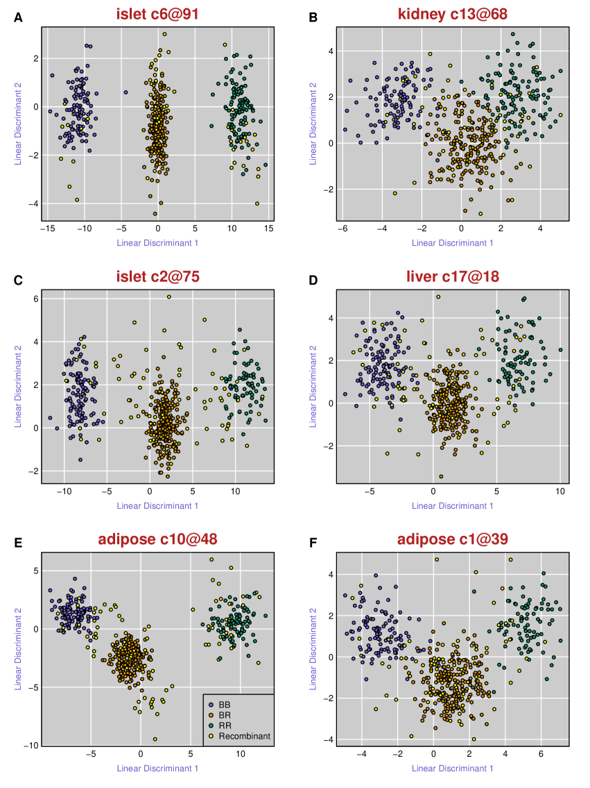
Figure 3: Scatterplots of the first two linear discriminants from application of linear discriminant analysis to the 100 expression traits that map to the region with the highest LOD score, with mice that show no recombination event in the region of a trans-eQTL hotspot. Blue, orange, and green points correspond to the non-recombinant mice with genotype BB, BR, and RR, respectively, at the eQTL. Yellow points correspond to recombinant mice.

For the islet chromosome 6 hotspot, the non-recombinant mice form three distinct clusters, and the recombinant mice (in yellow) fit reasonably well within those clusters (Figure 3A). This is consistent with there being a single eQTL.

For the islet chromosome 2 (Figure 3C) and adipose chromosome 10 (Figure 3E) hotspots, the non-recombinant mice again form tight clusters, but the recombinant mice fall clearly outside those clusters. This is evidence for the presence of more than one eQTL.

In the other three cases, kidney chromosome 13 (Figure 3B), liver chromosome 17 (Figure 3D), and adipose chromosome 1 (Figure 3F), the clusters of non-recombinants are not so tight, and the recombinants are not obviously different from the recombinants. However, for the liver chromosome 17 hotspot (Figure 3D), one might make the case that the majority of recombinants are at the boundaries between the clusters, and so multiple eQTL may be indicated.

Returning to the adipose chromosome 10 hotspot (Figure 3E), note how the recombinant mice form tight clusters that are distinct from the non-recombinants. If there are two eQTL in the region, perhaps these clusters correspond to different two-locus recombinant genotypes? Through the fit of a two-QTL model (in the next section), we estimate the two QTL to be at 48 and 54 cM. If we color the points by the two-locus genotypes for these two positions, we see that the clusters of non-recombinants do share a common two-locus genotype (Figure 4A).

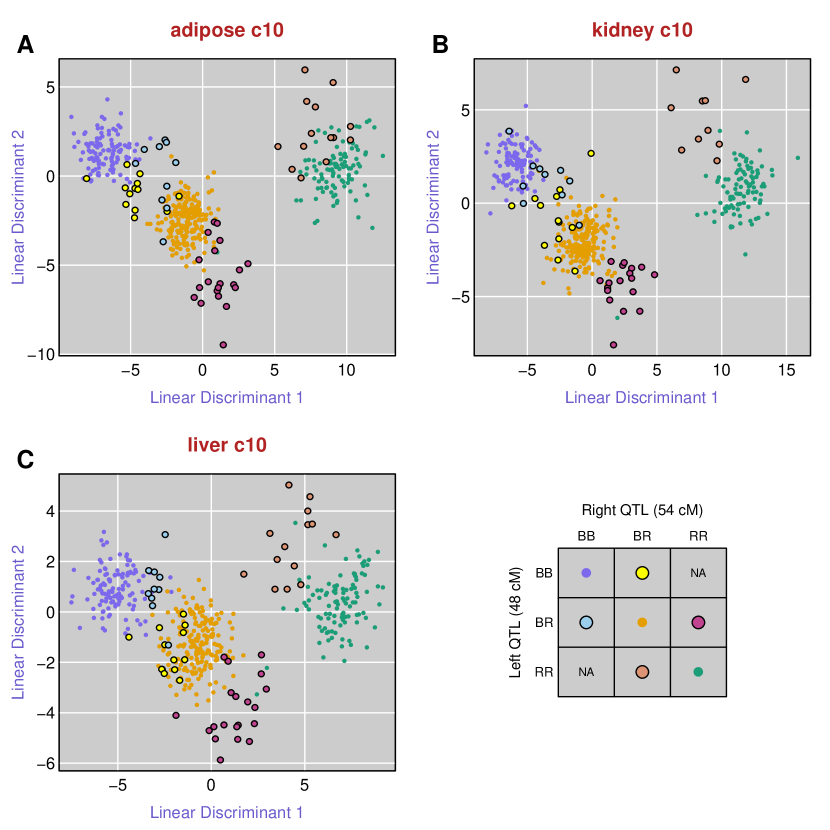
Figure 4: Scatterplots of the first two linear discriminants, as in Figure 3E, for the trans-eQTL hotspot on chromosome 10, here considering three tissues: adipose, kidney, and liver. Points correspond to mice, and they are colored according to their two-locus genotypes, for the inferred two QTL model, with one locus at $\sim$48 cM and the other at $\sim$54 cM.

This chromosome 10 hotspot also shows effect in kidney and liver, and so we applied this technique for this same region, with expression data for these tissues (Figures 4B and 4C). The three tissues give consistent results. Mice that are heterozygous at one QTL and homozygous BB at the other (yellow and light blue) sit between the non-recombinants that are homozygous BB (dark blue) and those that are heterozygous (orange). Mice that are homozygous RR at the left QTL and heterozygous at the right QTL (brown) sit above the non-recombinant RR mice (green), while mice that are heterozygous at the left QTL and homozygous RR at the right QTL (red) sit below the non-recombinant heterozygotes (orange).

There is one green point (non-recombinant RR) sitting among the red points (BR at the left QTL and RR at the right QTL). This mouse (with ID 3117) has a recombination event just to the left of the left QTL; if we moved that QTL slightly to the left, it would become a red point (BR at the left QTL and RR at the right QTL). In principle, a series of graphs of this form, with varying locations for the left and right QTL, could be used to define the QTL intervals in the context of this two-QTL model.

There is one additional green point among the red points in Figure 4C (liver). This mouse (with ID 3317) sits at the center of the cluster of green points in each of Figures 4A and 4B, and shows no recombination event in the region of these two QTL.

This example illustrates that consideration of the two-locus genotypes can help to strengthen evidence for two loci underlying a trans-eQTL hotspot. However, as we will describe below, in this particular case, the right eQTL appears to affect just three of the expression traits. Just one single trait, if affected by a separate locus, can have a great deal of leverage on these sorts of plots.

Formal tests for two QTL

To supplement these visualization techniques, we developed a formal statistical test for whether a trans-eQTL hotspot harbors one vs two eQTL. The results of this approach, for the six hotspots under consideration, are displayed in Figure 5.

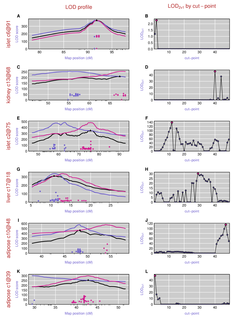
Figure 5: Results of a test of one versus two QTL at a trans-eQTL hotspot, considering the top 50 traits, in terms of LOD score, that map to the region. Each row is a hotspot. In the left panels, the black curve is the LOD curve for the single-QTL model, with estimated QTL location indicated by a black triangle. The blue and pink curves are profile LOD curves for the left and right QTL, respectively, for the estimated two-QTL model(with the estimated cut-point). Points indicate the LOD score and estimated QTL position for the 50 expression traits, analyzed separately. The points are colored according to whether they are estimated to be affected by the left QTL (blue) or right QTL (pink). The right panels show the $\text{LOD}_{2v1}^{(c)}$ score, indicating evidence for two versus one QTL, for each possible cut-point, $c$, of the list of expression traits into those that map to the left and those that map to the right QTL.

Let’s begin by considering the kidney chromosome 13 hotspot (Figures 5C and 5D). For these multivariate likelihood analyses, we focus on the top 50 expression traits mapping to the region, in terms of their LOD scores when considered individually. In the left panel (Figure 5C), the black curve is the LOD curve for the multivariate QTL analysis with a single-QTL model. The estimated QTL location is at 67.4 cM. The blue and pink curves are LOD profiles for the estimated two-QTL model, for which the estimated QTL locations are at 54.8 and 67.8 cM. The blue and pink points indicate the LOD scores and estimated QTL locations for the individual expression traits, with blue points affected by the left QTL and pink points affected by the right QTL. The right panel (Figure 5D) shows the evidence for two versus one QTL as a function of the choice of cut-point for the list of expression traits, into those affected by the left and right QTL. The inferred cut-point has 40 traits affected by the left QTL and 10 traits affected by the right QTL, and has a LOD_2v1 score of 45.8, indicating very strong evidence for two QTL, and for this particular cut-point.

The results for the islet chromosome 6 hotspot are displayed in Figures 5A and 5B. The inferred two-QTL model has QTL at 91.4 and 91.8 cM, with only the two expression traits affected by the left QTL. And LOD_2v1 = 2.3, indicating weak evidence for two QTL.

The results for the islet chromosome 2 hotspot (Figures 5E and 5F) indicate strong evidence for two QTL, with LOD_2v1 = 139. The estimated QTL are at 62.9 and 75.7 cM. The left QTL is inferred to affect 12 of the 50 expression traits.

The liver chromosome 17 hotspot (Figures 5G and 5H) has strong evidence for two QTL, with LOD_2v1 = 30, and the estimated QTL locations at 10.8 and 13.0 cM. The choice of cut-point of the expression traits is not so clear. We estimate 29 of the expression traits are affected by the left eQTL, but a model with 32 traits affected by the left eQTL gives a similar likelihood.

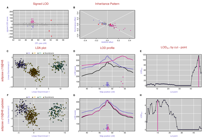
Figure S2: Effect of omitting three transcripts from the chromosome 10 trans-eQTL hotspot on the analysis results. A: Signed LOD scores, with transcripts having LOD $\geq$ 10 highlighted. The three transcripts to be omitted are indicated with X’s. B: Scatterplot of dominanance versus additive effects, with transcripts having LOD $\geq$ 10 highlighted. The three transcripts to be omitted are again indicated with X’s. C-E: LDA and likelihood results, as in Figures 3 and 5. F-H: LDA and likelihood results with the three transcripts omitted.

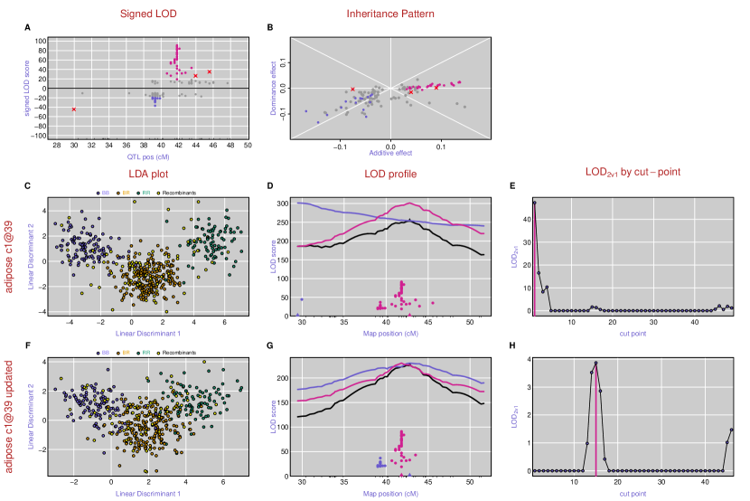
Figure S3: Effect of omitting one transcript from the chromosome 1 trans-eQTL hotspot on the analysis results. A: Signed LOD scores, with transcripts having LOD $\geq$ 10 highlighted. The transcript to be omitted is indicated with an X. B: Scatterplot of dominanance versus additive effects, with transcripts having LOD $\geq$ 10 highlighted. The transcript to be omitted is again indicated with an X. C-E: LDA and likelihood results, as in Figures 3 and 5. F-H: LDA and likelihood results with one transcript omitted.

For the adipose chromosome 10 (Figures 5I and 5J) and the adipose chromosome 1 (Figures 5K and 5L) hotspots, the evidence for two QTL is strong, but only three eQTL are inferred to be affected by the right eQTL at the chromosome 10 hotspot, and only 1 trait is inferred to be affected by the left eQTL at the chromosome 1 hotspot. If we trim off these expression traits and apply the procedure again, we find that, for the adipose chromosome 10 locus (see Figure S2), there is little evidence for more than one eQTL affecting the remaining traits. Further, the analysis of two-locus genotypes in the LDA plot in Figure 4 is largely driven by these three expression traits that map to 54 cM. Similarly, if we trim off the first expression trait for the adipose chromosome 1 hotspot (Figure S3), there is limited evidence for multiple QTL affecting the remaining traits.

In summary, the formal statistical test provides strong evidence for two eQTL in five of these six cases, but in two of the cases, the majority of the traits are affected by a single eQTL.

Simulations

To further assess the performance of the proposed likelihood-based test for whether a trans-eQTL hotspot harbors more than one eQTL, we performed a set of computer simulation studies.

We generated 500 intercross offspring with 100 markers on a 100 cM chromosome, and then simulated $p$ = 10 or 40 traits, with half of the traits affected by a QTL at 50 cM and the other traits affected by a QTL 0 -- 20 cM away (at 50 -- 70 cM). We also considered an unbalanced case with 5 traits affected by the left QTL and 35 traits affected by the right QTL. We assumed additive allele effects, with the additive effect of each QTL being $a$ = 0.1, 0.2, 0.3, 0.4, or 0.5. Residual variation followed a normal distribution with mean 0 and standard deviation 1, with traits conditionally independent given the QTL genotypes.

We used 100 simulation replicates for each situation and calculated P-values by a parametric bootstrap with 1000 simulation replicates.

The estimated power to detect two linked QTL, as a function of the distance between the QTL, is shown in Figure 6. When the QTL effect is smaller than 0.3, the power to distinguish two QTL within distance of 10 cM is low for $p=10$. For any fixed effect, the power to detect two QTL is higher for $p=40$ than for $p=10$. When the QTL effect is larger than 0.4, the power to distinguish two QTL separated by more than 5 cM is almost 100%.

The power to detect two QTL in the unbalanced case, with the left QTL affecting 5/40 traits, (Figure 6C) is considerably lower than for the balanced case (Figure 6B).

The case of distance = 0 corresponds to the null hypothesis of a single QTL affecting all traits. The power in this case is the type I error rate, and the parametric bootstrap method is seen to have somewhat inflated type 1 error rate, relative to the nominal 5%.

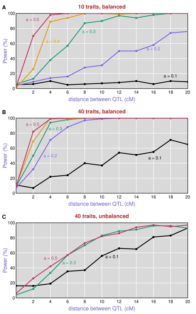
Figure 6: Power to detect two QTL as a function of the distance between the QTL, for varying QTL effects. (A) Ten traits, with each QTL affecting five traits. (B) 40 traits, with each QTL affecting 20, and (C) 40 traits, with the left QTL affecting five and the right QTL affecting 35.

Discussion

In this paper, we have proposed exploratory methods and a formal inference method for dissecting trans-eQTL hotspots. We applied these approaches to data on a large mouse intercross with gene expression microarray data on six tissues, and we performed a simulation study to investigate the performance of the formal inference method. Both the exploratory methods and the formal inference method are helpful in dissecting trans-eQTL hotspots, and can give improved estimates of the eQTL positions.

The exploratory methods have the advantage of providing insight into the underlying evidence for multiple eQTL: the multiple eQTL may show distinct inheritance patterns, or the recombinant and non-recombinant individuals may show differences in expression. However, while the visualization methods can be strongly informative, they will not necessarily reveal the presence of two eQTL, as the inheritance pattern of the two linked eQTL may be the same, or the first two linear discriminants may not be revealing of the difference between the recombinants and non-recombinants.

In forming a multivariate test statistic, we chose to follow the method of Knott and Haley (2000), but other multivariate analysis of variance (MANOVA) statistics could also be used, including Pillai’s trace, Lawley-Hotelling’s test, and Roy’s Lambda (Anderson 2003). Similarly, in the exploratory data visualization based on linear discriminant analysis, other dimension-reduction techniques could be used. A supervised (i.e., classification) method, which makes use of the known eQTL genotypes of the non-recombinant individuals, is preferred.

The main issue in the formal statistical test is the choice of expression traits, as we can’t handle a very large number of expression traits. Our choice to focus on the 50 traits with the highest LOD score was arbitrary, and deserves further investigation. Regularized methods (see Hastie et al. 2009, Sec 5.8), or a Bayesian approach, might have an advantage in this context. Such approaches could also be used to relax some of our modeling assumptions. For example, one might consider a model with two eQTL, where each expression trait can be affected by both.

We considered two methods to calculate p-values: a parametric bootstrap, and a stratified permutation test. The simulations to investigate power used the parametric bootstrap, and showed somewhat inflated type I error rate in the case. Moreover, neither approach takes account of the selection of hotspots, which may introduce further bias.

We considered a single tissue at a time. The joint consideration of multiple tissues could provide additional power to dissect trans-eQTL hotspots that are in common across tissues.

We ignored the effects of eQTL elsewhere in the genome and considered just one region in isolation. In doing so, the effects of any other eQTL become part of the residual variation. Local-eQTL are a particularly important case, as they are quite common and often have large effect. Controlling for the effect of local-eQTL could give better precision in the dissection of a trans-eQTL hotspot.

We have implemented our methods in an R package (R Core Team 2015), qtlpvl, available at https://github.com/jianan/qtlpvl.

FileS1.pdf  A 35-page PDF with the results as in Figures 2, 3, and 4, for all 35 trans-eQTL hotspots identified. (Available separately.)

Literature Cited

- Albert and Kruglyak (2015) Albert, F. W., and L. Kruglyak, 2015 The role of regulatory variation in complex traits and disease. Nat. Rev. Genet. 16: 197–212.
- Anderson (2003) Anderson, T. W., 2003 Testing the general linear hypothesis; multivariate analysis of variance. In An introduction to multivariate statistical analysis, chapter 8. Wiley, 3rd edition, 291–380.
- Breitling et al. (2008) Breitling, R., Y. Li, B. M. Tesson, J. Fu, C. Wu et al., 2008 Genetical genomics: spotlight on QTL hotspots. PLoS Genet. 4: e1000232.
- Brem et al. (2002) Brem, R. B., G. Yvert, R. Clinton, and L. Kruglyak, 2002 Genetic dissection of transcriptional regulation in budding yeast. Science 296: 752–755.
- Broman (2001) Broman, K. W., 2001 Review of statistical methods for QTL mapping in experimental crosses. Lab Animal 30: 44–52.
- Broman and Sen (2009) Broman, K. W., and S. Sen, 2009 A guide to QTL mapping with R/qtl. Springer, New York.
- Broman et al. (2003) Broman, K. W., H. Wu, S. Sen, and G. A. Churchill, 2003 R/qtl: QTL mapping in experimental crosses. Bioinformatics 19: 889–890.
- Carter and Falconer (1951) Carter, T. C., and D. S. Falconer, 1951 Stocks for detecting linkage in the mouse, and the theory of their design. J. Genet. 50: 307–323.
- Chesler et al. (2005) Chesler, E. J., L. Lu, S. Shou, Y. Qu, J. Gu et al., 2005 Complex trait analysis of gene expression uncovers polygenic and pleiotropic networks that modulate nervous system function. Nat. Genet. 37: 233–242.
- Fusi et al. (2012) Fusi, N., O. Stegle, and N. D. Lawrence, 2012 Joint modelling of confounding factors and prominent genetic regulators provides increased accuracy in genetical genomics studies. PLoS Comp. Biol. 8: e1002330.
- Gagnon-Bartsch and Speed (2012) Gagnon-Bartsch, J. A., and T. P. Speed, 2012 Using control genes to correct for unwanted variation in microarray data. Biostatistics 13: 539–552.
- Haley and Knott (1992) Haley, C. S., and S. A. Knott, 1992 A simple regression method for mapping quantitative trait loci in line crosses using flanking markers. Heredity 69: 315–324.
- Hastie et al. (2009) Hastie, T., R. Tibshirani, and J. Friedman, 2009 The elements of statistical learning: data mining, inference and prediction. Springer, New York, 2nd edition.
- Jansen (2007) Jansen, R. C., 2007 Quantitative trait loci in inbred lines. In D. Balding, M. Bishop and C. Cannings, editors, Handbook of Statistical Genetics, volume 1. Wiley, Chichester, 3rd edition, 589–622.
- Jansen and Nap (2001) Jansen, R. C., and J. P. Nap, 2001 Genetical genomics: the added value from segregation. Trends Genet. 17: 388–391.
- Jiang and Zeng (1995) Jiang, C., and Z. B. Zeng, 1995 Multiple trait analysis of genetic mapping for quantitative trait loci. Genetics 140: 1111–1127.
- Kang et al. (2008) Kang, H. M., C. Ye, and E. Eskin, 2008 Accurate discovery of expression quantitative trait loci under confounding from spurious and genuine regulatory hotspots. Genetics 180: 1909–1925.
- Keller et al. (2008) Keller, M. P., Y. Choi, P. Wang, D. B. Davis, M. E. Rabaglia et al., 2008 A gene expression network model of type 2 diabetes links cell cycle regulation in islets with diabetes susceptibility. Genome Res. 18: 706–716.
- Knott and Haley (2000) Knott, S. A., and C. S. Haley, 2000 Multitrait least squares for quantitative trait loci detection. Genetics 156: 899–911.
- Leek and Storey (2007) Leek, J. T., and J. D. Storey, 2007 Capturing heterogeneity in gene expression studies by surrogate variable analysis. PLoS Genet. 3: 1724–1735.
- Listgarten et al. (2010) Listgarten, J., C. Kadie, E. E. Schadt, and D. Heckerman, 2010 Correction for hidden confounders in the genetic analysis of gene expression. Proc. Natl. Acad. Sci. USA 107: 16465–16470.
- Nadeau and Frankel (2000) Nadeau, J. H., and W. N. Frankel, 2000 The roads from phenotypic variation to gene discovery: mutagenesis versus QTLs. Nat. Genet. 25: 381–384.
- R Core Team (2015) R Core Team, 2015 R: A Language and Environment for Statistical Computing. R Foundation for Statistical Computing, Vienna, Austria.
- Schadt et al. (2003) Schadt, E. E., S. A. Monks, T. A. Drake, A. J. Lusis, N. Che et al., 2003 Genetics of gene expression surveyed in maize, mouse and man. Nature 422: 297–302.
- Stegle et al. (2010) Stegle, O., L. Parts, R. Durbin, and J. Winn, 2010 A Bayesian framework to account for complex non-genetic factors in gene expression levels greatly increases power in eQTL studies. PLoS Comp. Biol. 6: e1000770.
- Tian et al. (2015) Tian, J., M. P. Keller, A. T. Oler, M. E. Rabaglia, K. L. Schueler et al., 2015 Identification of Slco1a6 as a candidate gene that broadly affects gene expression in mouse pancreatic islets. Genetics 201: 1253–1262.
- Yvert et al. (2003) Yvert, G., R. B. Brem, J. Whittle, J. M. Akey, E. Foss et al., 2003 Trans-acting regulatory variation in Saccharomyces cerevisiae and the role of transcription factors. Nat. Genet. 35: 57–64.
- Zeng et al. (2000) Zeng, Z.-B., J. Liu, L. F. Stam, C.-H. Kao, J. M. Mercer et al., 2000 Genetic architecture of a morphological shape difference between two Drosophila species. Genetics 154: 299–310.
The dissection of expression quantitative trait locus hotspots
SUPPLEMENT
Jianan Tian∗,
Mark P. Keller†,
Aimee Teo Broman‡,
Christina Kendziorski‡,
Brian S. Yandell∗,§,
Alan D. Attie†
Karl W. Broman‡,1
Departments of ∗Statistics, †Biochemistry, ‡Biostatistics and Medical Informatics, and §Horticulture,