Turbulent mixing: matching real flows to Kraichnan flows

Abstract

Majority of theoretical results regarding turbulent mixing are based on the model of ideal flows with zero correlation time. We discuss the reasons why such results may fail for real flows and develop a scheme which makes it possible to match real flows to ideal flows. In particular we introduce the concept of mixing dimension of flows which can take fractional values. For real incompressible flows, the mixing dimension exceeds the topological dimension; this leads to a local inhomogeneity of mixing — a phenomenon which is not observed for ideal flows and has profound implications, for instance impacting the rate of bimolecular reactions in turbulent flows. Finally, we build a model of compressible flows which reproduces the anomalous Lyapunov exponent values observed for time-correlated flows by Boffetta et al (2004), and provide a qualitative explanation of this phenomenon.

Turbulent mixing affects us in many ways, for instance via weather and Solar storms. Here we assume that the fields which are being mixed are passive, i.e. do not affect the statistical properties of the underlying velocity field. Examples of fairly passive fields include fluid temperature, concentration of pollutants, nutrients, etc., and weak magnetic fields at a linear stage of magnetic dynamos; more examples can be found in reviews Falkovich et al. (2001); Sreenivasan and Antonia (1997); Warhaft (2000); Dimotakis (2005); Shraiman and Siggia (2000); Toschi and Bodenschatz (2009); Grabowski and Wang (2013); Brandenburg and Subramanian (2005).

Analytical studies of turbulent mixing have been mostly based on the Kraichnan’s model Kraichnan (1994), which assumes the velocity field to be $\delta$-correlated in time (with vanishing correlation time). This approach has been successful because properties of turbulently mixed fields depend almost exclusively on the stretching statistics of the material elements (point pair separations, lines, surface areas, volumes) as a function of time; hence, as long as Kraichnan flows match the stretching statistics of real flows, the predictions based on them will be accurate. Therefore, the finding that for compressible flows, e.g. at the surface of turbulent fluids, Kraichnan’s model fails in basic qualitative predictions Boffetta et al. (2004); Larkin and Goldburg (2010) has raised a major theoretical challenge which remained open regardless of recent studies of the role of time correlations, cf. Gustavsson and Mehlig (2013); Dhanagare et al. (2014); Jurčišinová and Jurčišin (2013); Duplat and Villermaux (2000); Falkovich and Afonso (2007).

One can show (e.g. using the approaches of Balkovsky and Fouxon (1999); Boldyrev and Schekochihin (2000); Kalda (2000)) that asymptotically, when the observation time becomes much greater than the flow correlation time, the probability distributions of the logarithms of the dimensions of a material parallelepiped become Gaussian. Both the median and variance of such a Gaussian distribution grow linearly in time, the median’s speed is the Lyapunov exponent $\lambda_{i}$; half of the variance growth rate will be called as the Lyapunov exponent diffusivity and denoted by $\varkappa_{i}$. Here, $i=1$ refers to the length, $i=2$ — to the face height, and $i=3$ — to the height of a material parallelepiped. Thus, the stretching statistics is fully described by the set of exponents $\lambda_{i},\kappa_{i}$, $i=1\ldots d$ ($d$ denotes the flow dimensionality). Only “fat-tailed” time correlations (e.g. due to near-wall stagnant regions Gouillart et al. (2007)) can invalidate this scenario.

One of the listed exponents can be equated to unity with a proper choice of time unit. Thus, what defines the dynamics of passive fields are the ratios of the exponents. So, the efficiency of small-scale kinematic magnetic dynamos Gruzinov et al. (1996) and the exponent of the statistical conservation law for Lagrangian pair dispersion Falkovich and Frishman (2013); Frishman et al. (2015) depend on the ratio $\lambda_{1}/\varkappa_{1}$ ; multifractal spectra of scalar dissipation fields depend on $\lambda_{d}/\varkappa_{d}$ Kalda (2000), the same applies to the dynamics of monomolecular reactions in compressible flows Kalda (2011); the (multi)fractal properties of tracer fields in compressible 2-dimensional (2D) flows depend on $\lambda_{2}/\lambda_{1}$ Bec et al. (2004); Boffetta et al. (2004).

The structure of this Letter is as follows. For statistically isotropic homogeneous Kraichnan flows, the exponent ratios are expressed via the flow compressibility and dimensionality Falkovich et al. (2001); first we discuss different factors contributing to the failure of these expressions for real flows. Further, we introduce a class of model flows; based on this model in 2D geometry, we obtain expressions for $\lambda_{1}/\varkappa_{1}$ and $\lambda_{1}/\lambda_{2}$ which exhibit non-universality depending not only on the Kubo number $K$ (ratio of the correlation time and small-scale eddy turnover time), but also on the statistics of the determinant of the velocity gradient tensor. We use qualitative arguments to show that the results are robust and not limited to our model. Based on the fact that for incompressible Kraichnan flows, $\lambda_{1}/\varkappa_{1}=d$, the ratio $\lambda_{1}/\varkappa_{1}\equiv d_{m}$ will be called the mixing dimension of the flow; we argue that for time-correlated flows, $d_{m}>d$, and discuss implications of this inequality. Finally, we show that when exponents are averaged over a realistic ensemble of determinant values, the contradiction between the theory and experimental findings Boffetta et al. (2004); Larkin and Goldburg (2010) becomes resolved.

Factor A: different correlation times for potential and solenoidal components. The mismatch between real and Kraichnan flows can be caused by the solenoidal and potential components (denoted as $\boldsymbol{v}_{s}$ and $\boldsymbol{v}_{p}$) of the Helmholtz decomposition of the velocity field $\boldsymbol{v}\equiv\boldsymbol{v}(\boldsymbol{r},t)$ having different correlation times $\tau_{s}$ and $\tau_{p}$, respectively. For instance in marine environment, the potential component of surfaces flow is associated with up- and down-welling, and is often persistent due to being caused by bathygraphy Kalda et al. (2014). However, we can modify the Kraichnan model so as to cover the case $\tau_{s}\neq\tau_{p}$ if we introduce very small correlation times $\tau_{s},\tau_{p}$. Then, for statistically isotropic homogeneous case with $\tau_{s}=\tau_{p}\equiv\tau$,

$$\lambda_{i} =D_{1}\left\{d(d-2i+1)-2\wp[d+(d-2)i]\right\},$$

$$\varkappa_{i} =D_{1}(d-1)(1+2\wp),$$ (1)

where the compressibility $\wp\equiv{\cal F}_{p}/{\cal F}$ is defined via the mean squared Frobenius norms ${\cal F}_{p}\equiv\langle\|\boldsymbol{\nabla v}_{p}\|^{2}\rangle=\mbox{$\langle(\boldsymbol{\nabla}\cdot\boldsymbol{v})^{2}\rangle$}$, and ${\cal F}\equiv\langle\|\boldsymbol{\nabla v}\|^{2}\rangle$; the factor $D_{1}=\frac{{\cal F}\tau}{d(d-1)(d+2)}$, where $\tau=\frac{1}{\cal F}\int_{0}^{\infty}\langle\partial_{i}v_{j}(\boldsymbol{r},0)\partial_{i}v_{j}(\boldsymbol{r},t)\rangle\mathrm{d}t$, cf. Falkovich et al. (2001). If we substitute in this integral $\boldsymbol{v}=\boldsymbol{v}_{p}+\boldsymbol{v}_{s}$ and assume $\tau_{s}\neq\tau_{p}$, Eq. (1) is generalized to $\lambda_{i}={\cal F}_{s}\tau_{s}\frac{d-2i+1}{(d-1)(d+2)}+{\cal F}_{p}\tau_{p}\frac{d-4i}{d(d+2)}$, and $\varkappa_{i}={\cal F}_{s}\tau_{s}\frac{1}{d(d+2)}+{\cal F}_{p}\tau_{p}\frac{3}{d(d+2)}$, where ${\cal F}_{s}\equiv\langle\|\boldsymbol{\nabla v}_{s}\|^{2}\rangle$. Now it becomes clear that for the exponent ratios to depend only on $\wp$ and $d$, and for Eq. (1) to remain valid with $D_{1}=\frac{{\cal F}_{s}\tau_{s}+{\cal F}_{p}\tau_{p}}{d(d-1)(d+2)}$, the compressibility needs to be defined as

$$\wp=\tilde{\wp}\equiv{\cal F}_{p}\tau_{p}/({\cal F}_{s}\tau_{s}+{\cal F}_{p}\tau_{p}).$$ (2)

Our simulations with 2D sine flow (velocity field is sinusoidal in space and a discretely updated random function in time, cf. Supplementing Material Ain ) show that for Kubo number $K=\tau\sqrt{\cal F}\ll 1$, the generalized expression of compressibility $\tilde{\wp}$ describes adequately flows with $\tau_{p}\neq\tau_{s}$, see Fig. 1. However, for $K\sim 1$, a considerable mismatch is observed, confirming the findings of ref. Boffetta et al. (2004).

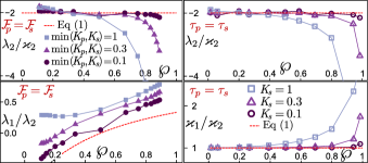
Figure 1: Lyapunov exponent ratios from simulations with sine flows are plotted versus the compressibility $\wp$ as defined by Eq. (2). Left column: solenoidal and potential velocity components obey equal norms but different correlation times; right column: while $\tau_{p}=\tau_{s}$, norms are different.

Factor B: correlations along Lagrangian trajectories due to particles embedded into material volumes. Hypersonic flows, if judged by velocity gradient, are characterized by a considerable compressibility; however, the sum of Lyapunov exponents is strictly zero (limitlessly contracting volumes would imply limitlessly growing pressure fluctuations). This violates Eq. (1) which predicts $\sum_{i}\lambda_{i}=-D_{1}d(d-1)(d+2)\wp$. The mismatch is explained by long-term correlations.

Factor C: genuine finite correlation time effects. Even if the factor A is accounted for by using generalized compressibility (2), and the factor B is negligible, time correlations can cause a considerable departure from Eq. (1). We follow the approach developed in Kalda (2000, 2007) and apply multiplicatively the deformations achieved during a correlation time $\tau$ assuming that beyond a correlation time, the correlations are negligible. Then, infinitesimal material vectors $\boldsymbol{\textrm{d}x}$ are transformed according to the tensor $\hat{\mathcal{D}}_{t}=\exp({\int_{t}^{t+\tau}\boldsymbol{\nabla}\boldsymbol{v}\textrm{d}t^{\prime}})$, $\boldsymbol{\textrm{d}x}_{n\tau}=\prod_{j=0}^{n-1}\hat{\mathcal{D}}_{j\tau}\cdot\boldsymbol{\textrm{d}x}_{0}$.

First, let us consider incompressible flows. In the case of 2D geometry, we need to study just the normalized length of the vector $\ell_{t}\equiv|\boldsymbol{\textrm{d}x}_{t}|/|\boldsymbol{\textrm{d}x}_{0}|$. Indeed, at the limit $t\to\infty$, $\lambda_{1}=\frac{1}{t}\langle\ln\ell_{t}\rangle$ and $\varkappa_{1}=\frac{1}{2t}\langle(\ln\ell_{t}-\lambda_{1}t)^{2}\rangle$. A square built on $\boldsymbol{\textrm{d}x}$ evolves into a parallelogram of normalized height $h_{t}$ and constant surface area, $\ell_{t}h_{t}=1$, therefore $\lambda_{2}=\frac{1}{t}\langle\ln h_{t}\rangle=-\lambda_{1}$ and $\varkappa_{2}=\varkappa_{1}$. Furthermore, the increments $\ln\ell_{t}-\ln\ell_{t-\tau}$ and $\ln\ell_{t+\tau}-\ln\ell_{t}$ are uncorrelated, hence $\lambda_{1}\equiv\lim_{t\to\infty}\frac{1}{t}\langle\ln\ell_{t}\rangle=\frac{1}{\tau}\langle\ln\ell_{\tau}\rangle$ and similarly, $\varkappa_{i}=\frac{1}{2\tau}\langle(\ln\ell_{\tau}-\lambda_{1}\tau)^{2}\rangle$. Averages $\langle\ln\ell_{\tau}\rangle$ and $\langle(\ln\ell_{\tau})^{2}\rangle$ will be calculated in two stages: averaging over rotations of a fixed tensor $\hat{\mathcal{D}}_{\tau}\equiv\hat{\mathcal{D}}$ (using statistical isotropy), and averaging over an ensemble of matrices $\hat{\mathcal{D}}$.

For a fixed transformation tensor $\hat{\mathcal{D}}$, $\ell_{\tau}^{2}=\boldsymbol{e}^{T}\hat{\mathcal{D}}^{T}\hat{\mathcal{D}}\boldsymbol{e}$, where $\boldsymbol{e}\equiv\textrm{d}\boldsymbol{x}/|\textrm{d}\boldsymbol{x}|$. The (Green’s) deformation tensor $\hat{\mathcal{D}}^{T}\hat{\mathcal{D}}$ is symmetric and positive semidefinite, hence, it has non-negative eigenvalues $p^{2}$ and $q^{2}$ ($q=1/p$ if $\wp=0$), and is diagonalizable via a rotation into $\operatorname{diag}(p^{2},q^{2})$. Thus, $\ell_{\tau}^{2}=p^{2}\cos^{2}\alpha+q^{2}\sin^{2}\alpha$, and

$$\lambda_{1}\tau=\int_{0}^{\frac{\pi}{2}}\ln\ell_{\tau}^{2}\,\frac{\textrm{d}\alpha}{\pi}=\ln\frac{p+q}{2}\text{,}$$ (3)

$$\varkappa_{1}\tau=\int_{0}^{\frac{\pi}{2}}\left(\ln\ell_{\tau}^{2}\right)^{2}\frac{\textrm{d}\alpha}{4\pi}-\frac{\lambda_{1}^{2}\tau^{2}}{2}=\frac{1}{4}\operatorname{Li}_{2}\!\frac{(p-q)^{2}}{(p+q)^{2}}\text{,}$$ (4)

where $\operatorname{Li}_{2}x=-\int_{0}^{x}\left[\ln(1-u)\right]\,\frac{\textrm{d}u}{u}$ is the dilogarithm, and $p\geq q>0$. The integral of Eq.(3) has been tabulated in (Prudnikov et al., 1981, Eq. 2.6.38.4), and derived in Ainsaar and Kalda (2015); the one of Eq. (4) is derived in the Supplementing Material Ain .

Using Eqns. (3,4), we have plotted the mixing dimension as a function of the parameter $p$ (Fig. 2, insert), which demonstrates non-universality. Indeed, we see that $d_{m}$ grows limitlessly with $p$, and $p$, in its term, can take arbitrarily large values if $K$ is large enough. In order to understand how $d_{m}$ depends on the velocity gradient statistics, we assume simplifyingly that $\boldsymbol{\nabla v}$ remains constant during one correlation time [$\boldsymbol{\nabla v}(t)\equiv\boldsymbol{\nabla v}_{1}$], upon which it obtains a new random value. Real flows, of course, depend smoothly on time, but $\boldsymbol{\nabla v}_{1}$ can be interpreted as such a time-averaged tensor $\boldsymbol{\nabla v}(t)$ that during one correlation time, it results in the same deformation tensor $\hat{\mathcal{D}}^{T}\hat{\mathcal{D}}$ as the real smooth-in-time flow. Statistically homogeneous flows include both saddles ($\det\boldsymbol{\nabla v}<0$) and extrema ($\det\boldsymbol{\nabla v}>0$) of the streamfunction and $\left<\det\boldsymbol{\nabla v}\right>=0$. The smallest possible ensemble of tensors $\boldsymbol{\nabla v}$ satisfying this constraint includes two fixed tensors $\boldsymbol{\nabla v}_{1}$ and $\boldsymbol{\nabla v}_{2}$ with $\det\boldsymbol{\nabla v}_{1}+\det\boldsymbol{\nabla v}_{2}=0$; the main graph of Fig. 2 shows the behavior of $d_{m}$ for such ensembles. For $K\ll 1$, the values of $d_{m}$ remain close to (and larger than) the Kraichnan limit value $d=2$. For $K\gtrsim 1$, much larger values can be reached.

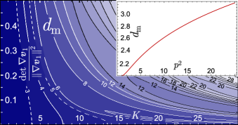
Figure 2: Mixing dimension $d_{m}\equiv\lambda_{1}/\varkappa_{1}$ of 2D incompressible model flows (with fixed values of $\frac{|\det\nabla\boldsymbol{v}_{1}|}{\|\nabla\boldsymbol{v}_{1}\|}$) as a function of the determinant of the velocity gradient and the Kubo number $K\equiv\tau\|\boldsymbol{\nabla v}_{1}\|$; curves denote isolines and are labeled with the values of $d_{m}$. Insert: $d_{m}$ versus the transformation tensor’s singular value $p$.

Let us discuss now the significance of the mixing dimension $d_{m}\equiv\lambda_{1}/\varkappa_{1}$. First we show that for incompressible Kraichnan flows we need to have $d_{m}=d$. Let $\mu\equiv\ln r/r_{0}$ denote the distance of tracer particles, initially seeded at a small distance $r_{0}$, using logarithmic scale. Then, $\mu$ performs a biased random walk with mean velocity $\lambda_{1}$ and diffusivity $\varkappa_{1}$; the step length is defined by the correlation time of the flow, cf. Kalda (2007). Thus, the asymptotic-in-time evolution equation for the distribution function $\sigma=\sigma(\mu,t)$ is written as $\partial_{t}\sigma+\lambda_{1}\partial_{\mu}\sigma=\varkappa_{1}\partial^{2}_{\mu}\sigma$. The distance $r$ is limited by inter-molecular distances $r_{\min}$, hence we need to apply a reflective boundary condition at $\mu_{\min}=\ln r_{\min}/r_{0}$; this leads to a quasi-stationary distribution $\sigma\propto\textrm{e}^{d_{m}\mu}$ at small values of $\mu$ if we wait long enough ($t\gtrsim|\mu_{\min}|/\lambda_{1}$). Therefore, the cumulative distribution function in $r$-space is proportional to $r^{d_{m}}$.

Now, consider the dye distribution around a material point $P$, with a spot of dye being seeded initially at a small distance $r_{0}$ from it. Equality $d=d_{m}$ implies a locally homogeneous mixing: the amount of dye inside a sphere around $P$ scales as the volume of the sphere. Inequality $d_{m}<d$ is clearly impossible for incompressible flows as it would mean local clustering of the material particles. Meanwhile, $d_{m}>d$ implies local inhomogeneity in mixing: with a high probability, a neighborhood of $P$ is left without dye. This scenario cannot be realized (hence, $d=d_{m}$) in the case of Kraichnan flows when the material deformations are diffusive in nature. Indeed, at small time-scales, diffusion dominates over the mean drift in the dynamics of $\mu\equiv\ln r/r_{0}$, and therefore, the distance $\Delta\mu=\ln r_{0}/r_{\min}$ to the reflection point of $\mu$ is traveled diffusively. This ensures that all those dye particles which start from the vicinity of $P$ will also visit the smallest neighborhood of $P$, i.e. there is a locally homogeneous mixing described by $\sigma\propto r^{d}$. Meanwhile, for real flows, diffusive behavior is reached only asymptotically, at time scales larger than $\tau$. So, there is a chance that with few initial steps, the dye particle “runs away” from the point $P$. At long time scales, drift dominates over diffusion; thus, if the dye particle managed to evade the point $P$ at the early stage, it will avoid it forever.

The case of compressible fields has been studied preliminarily in a technical report Ainsaar and Kalda (2015); here we use our model to explain the challenging findings of Ref. Boffetta et al. (2004) and provide a qualitative explanation of this phenomenon. To keep the overall area of the basin constant, both divergent and convergent regions need to be present simultaneously. We’ll use the same ensemble for $\boldsymbol{\nabla v}$ as before, with an additional requirement $\boldsymbol{\nabla}\cdot\boldsymbol{v}_{1}=-\boldsymbol{\nabla}\cdot\boldsymbol{v}_{2}\equiv\delta>0$. We assume simplifyingly that the convergent (‘C’) and divergent (‘D’) domains are separated with a sharp boundary which remains constant throughout the full correlation time $\tau$, upon which new random domain breakup and tensor rotation angles are coined. While this may seem to be an unrealistic simplification, we’ll argue later that our model captures essential features of realistic flows.

During one correlation time, some of the tracer particles are carried from domain ‘D’ to domain ‘C’, let us consider such particles which cross the domain boundary at the moment $t$ (measured from when the current domains were established), henceforth referred to as the $t$-particles. Eq. (3) allows us to average the Lyapunov exponent over $t$-particles, $\left<\lambda_{1}\right>_{t\textrm{-p}}\equiv\Lambda(t)=\frac{1}{\tau}\ln\left(\frac{p_{1}+q_{1}}{2}\frac{p_{2}+q_{2}}{2}\right)$; here $p_{1}$ and $q_{1}$ are the singular values of $\textrm{e}^{\boldsymbol{\nabla}\boldsymbol{v}_{1}(\tau-t)}$, and $p_{2}$ and $q_{2}$ are that of $\textrm{e}^{\boldsymbol{\nabla}\boldsymbol{v}_{2}t}$.

Within region ‘D’, surface areas grow exponentially $A\propto\textrm{e}^{\delta t}$, hence, the tracer density falls as $\textrm{e}^{-\delta t}$. Thus, the probability for a random particle to exit the region between $t$ and $t+\textrm{d}t$ is given by $\textrm{d}p=\textrm{e}^{-\delta t}\delta\textrm{d}t$. Now we can find the overall Lyapunov exponent by averaging $\Lambda(t)$ over all the tracer particles, $\lambda_{1}=\left<\Lambda(t)\right>=\frac{1}{2}\left[\int_{0}^{\tau}\Lambda(t)\delta\textrm{e}^{-\delta t}\textrm{d}t+\Lambda(\tau)\textrm{e}^{-\delta t}+\Lambda(0)\right]$. Here, the second and third terms correspond to those particles which remain for the whole period $\tau$ within ‘D’ and ‘C’, respectively. The area growth exponent $\lambda_{A}=\lambda_{1}+\lambda_{2}$ is calculated similarly: in region ‘D’, $\lambda_{A}=\delta$, and in region ‘C’, $\lambda_{A}=-\delta$. At the position of a $t$-particle, the area growth factor is $\textrm{e}^{\delta t-\delta(\tau-t)}$; once we average over all the values of $t\in\left[0,\tau\right]$, we end up with $\lambda_{A}=\frac{1}{\tau}\left(1-\delta\tau-e^{-\delta\tau}\right)$. Finally, we can express $\lambda_{2}=\lambda_{A}-\lambda_{1}$.

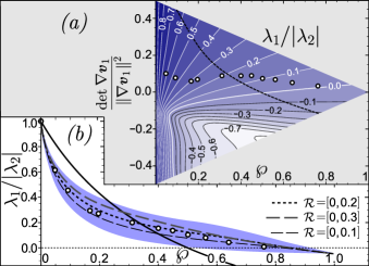
Figure 3: (a) $\lambda_{1}/|\lambda_{2}|$ as a function of $\wp$ and $\frac{\det\nabla\boldsymbol{v}_{1}}{\|\nabla\boldsymbol{v}_{1}\|^{2}}$ for $K=9$; numbers indicate the isoline values Graph area is triangular because for any $\nabla\boldsymbol{v}_{1}$, $\frac{2|\det\nabla\boldsymbol{v}_{1}|}{\|\nabla\boldsymbol{v}_{1}\|^{2}}\leq 1-\wp$. Dots show the intersection points of this graph with the data of Ref. Boffetta et al. (2004), and dashed curve — with the theoretical dependence for Kraichnan flows. (b) Shaded region shows the range of values of $\lambda_{1}/|\lambda_{2}|$ for $\frac{\det\nabla\boldsymbol{v}_{1}}{\|\nabla\boldsymbol{v}_{1}\|^{2}}\in[0,0.2]$; solid curve: theoretical dependence for Kraichnan flows; dots: data of Ref. Boffetta et al. (2004); dashed lines: the exponents are averaged over $\frac{\det\nabla\boldsymbol{v}_{1}}{\|\nabla\boldsymbol{v}_{1}\|^{2}}\in{\cal R}$, the ranges ${\cal R}$ being shown by the legend.

We used our expressions to compute $\frac{\lambda_{1}}{|\lambda_{2}|}$ as a function of the model parameters; in Fig. 3(a), the results are depicted for $K=9$. Dashed curve marks the intersection of this graph with the Kraichnan-limit-dependence $\frac{\lambda_{1}}{|\lambda_{2}|}=\frac{1-2\wp}{1+2\wp}$ and divides the plane into two regions: at the left-bottom part, $\frac{\lambda_{1}}{|\lambda_{2}|}$ is decreased due to time-correlations, and at the right-top part, the effect is opposite.

At small compressibilities [$\wp<0.1$ for Fig. 3(a)], $\frac{\lambda_{1}}{|\lambda_{2}|}$ is always reduced; we show that this is a robust feature, not bound to our model. Consider $\lambda_{1}$ as a function of $K$ for flows with a fixed probability distribution of $\boldsymbol{\nabla v}$: Eq. (1) holds while $K\ll 1$, and gives us estimate $\lambda_{1}\sim\tau{\cal F}=K\sqrt{\cal F}$. By $K\gg 1$, a saturation value is reached, which is estimated as the stretching rate near saddles, $\lambda_{1}\sim\sqrt{\cal F}$. Exponent $\lambda_{A}$ behaves similarly, but saturates later: for material areas, the Kraichan approximation holds as long as the area change during $\tau$ remains small, $\tau\boldsymbol{\nabla}\cdot\boldsymbol{v}=K\sqrt{\wp}\ll 1$, and yields $\lambda_{A}\sim-K\wp\sqrt{\cal F}$; for $K\sqrt{\wp}\gg 1$, saturation $\lambda_{A}\sim-|\boldsymbol{\nabla}\cdot\boldsymbol{v}|$ is reached. If $K\gtrsim 1$ and $\wp\lesssim K^{-2}$, saturation is reached for $\lambda_{1}$, but not for $\lambda_{A}$, i.e. $\frac{|\lambda_{2}|}{\lambda_{1}}=1-\frac{\lambda_{A}}{\lambda_{1}}\sim 1+K\wp$. This means that larger values of $K$ lead to faster growth of $\frac{|\lambda_{2}|}{\lambda_{1}}$ with $\wp$.

At larger compressibilities [$\wp\gtrsim 0.3$ for Fig. 3(a)], it can be approximately said that $\lambda_{1}>0$ for $\det\boldsymbol{\nabla}\boldsymbol{v}_{1}>0$ and $\lambda_{1}<0$ for $\det\nabla\boldsymbol{v}_{1}<0$. This is also a robust feature. Indeed, at the limit $K\gg 1$, the tracers stay mostly near the most convergent areas, hence $\lambda_{1}$ is dominated by the stretching statistics in the regions with smallest values of $\boldsymbol{\nabla}\cdot\boldsymbol{v}$. Therefore, we can assume that along Lagrangian trajectories, $\boldsymbol{\nabla}\boldsymbol{v}$ remains almost constant for a long period of time; under the assumption of constant $\boldsymbol{\nabla}\boldsymbol{v}$, one can show that $2\lambda_{1}=\boldsymbol{\nabla}\cdot\boldsymbol{v}+\operatorname{Re}\sqrt{(\boldsymbol{\nabla}\cdot\boldsymbol{v})^{2}-4\det\boldsymbol{\nabla}\boldsymbol{v}}$; hence, with $\boldsymbol{\nabla}\cdot\boldsymbol{v}<0$, the sign of $\lambda_{1}$ is opposite to that of $\det\boldsymbol{\nabla}\boldsymbol{v}$. In the case of our model flow, this corresponds to $\operatorname{sgn}\lambda_{1}=\operatorname{sgn}\det\boldsymbol{\nabla}\boldsymbol{v}_{1}$.

Boffetta et al.Boffetta et al. (2004) found the Lyapunov dimension $d_{L}=1+\lambda_{1}/|\lambda_{2}|$ as a function of $\wp$ for realistic compressible flows with numerically increased correlation time at $K\approx 9$. To compare our theory with Ref. Boffetta et al. (2004), Lyapunov exponents need to be averaged over a realistic ensemble of velocity gradients. We were unable to find data for free-slip liquid interfaces; thus, the analysis is based on the data for 2D slices of an incompressible 3D velocity field Cardesa et al. (2013); Rabey et al. (2015); these papers report the joint probability density of the trace (there called “$-p$”) and determinant (“$q$”) of the velocity gradient. There is a small difference in the normalization of $\det\nabla\boldsymbol{v}$: Refs. Cardesa et al. (2013); Rabey et al. (2015) normalize by $\langle(\nabla\times\boldsymbol{v})_{z}^{2}\rangle$. Based on the fact that before taking the slice their 3D velocity field $\boldsymbol{v}_{\mathrm{3D}}$ was incompressible, and assuming isotropy, it can be shown that our normalization factor is $\frac{4}{3}$ times larger. Keeping this in mind, Fig. 3 of Ref Cardesa et al. (2013) tells us that within regions ‘D’ with $p<0$, the values of $\frac{\det\nabla\boldsymbol{v}_{1}}{\|\nabla\boldsymbol{v}_{1}\|^{2}}$ remain mostly between 0 and 0.2. When we average the Lyapunov exponents over this range, our model provides a good match to the data of Ref. Boffetta et al. (2004), see Fig. 3 (bottom).

In conclusion, we have expressed the ratios of Lyapunov exponents and their diffusivities in terms of velocity gradient statistics, and introduced the mixing dimension $d_{m}$ as a characteristic of a flow. Those existing theories which are based on the values of these ratios (for instance Gruzinov et al. (1996); Bec et al. (2004)) become directly applicable to real time-correlated flows. We also pinpoint a major qualitative difference: while open Kraichnan flows are characterized by locally homogeneous mixing (once we wait long enough, dye density will be distributed evenly over a neighborhood of a fixed material point), in the case of time-correlated flows, the mixing is locally inhomogeneous. This difference stems from the fact that for Kraichnan flows, $d_{m}$ equals to the integer-valued topological dimension $d$, and cannot perfectly match real flows with fractional $d_{m}$. Such an inhomogeneity has major implications, in particular for the rate of bimolecular reactions with initially separated reagents (cf. Martinand and Vassilicos (2007); Ait-Chaalal et al. (2012)), for the mixing of different dyes (cf. recent experimental study Kree et al. (2013)), and for the efficiency of kinematic magnetic dynamos Gruzinov et al. (1996). The local inhomogeneity is also likely the reason behind non-universality of mixing with respect to the details of tracer injection Gotoh and Watanabe (2015).

The support of the EU Regional Development Fund Centre of Excellence TK124 (CENS) is acknowledged.

References

- Falkovich et al. (2001) G. Falkovich, K. Gawȩdzki, and M. Vergassola, Rev. Mod. Phys. 73, 913 (2001).
- Sreenivasan and Antonia (1997) K. R. Sreenivasan and R. A. Antonia, Annu. Rev. Fluid Mech. 29, 435 (1997).
- Warhaft (2000) Z. Warhaft, Annu. Rev. Fluid Mech. 32, 203 (2000).
- Dimotakis (2005) P. E. Dimotakis, Annu. Rev. Fluid Mech. 37, 329 (2005).
- Shraiman and Siggia (2000) B. I. Shraiman and E. D. Siggia, Nature 405, 639 (2000).
- Toschi and Bodenschatz (2009) F. Toschi and E. Bodenschatz, Annu. Rev. Fluid Mech. 41, 375 (2009).
- Grabowski and Wang (2013) W. W. Grabowski and L.-P. Wang, Annu. Rev. Fluid Mech. 45, 293 (2013).
- Brandenburg and Subramanian (2005) A. Brandenburg and K. Subramanian, Phys. Rep. 417, 1 (2005).
- Kraichnan (1994) R. H. Kraichnan, Phys. Rev. Lett. 72, 1016 (1994).
- Boffetta et al. (2004) G. Boffetta, J. Davoudi, B. Eckhardt, and J. Schumacher, Phys. Rev. Lett. 93, 134501 (2004).
- Larkin and Goldburg (2010) J. Larkin and W. I. Goldburg, Phys. Rev. E 82, 016301 (2010).
- Gustavsson and Mehlig (2013) K. Gustavsson and B. Mehlig, J. of Stat. Phys. 153, 813 (2013).
- Dhanagare et al. (2014) A. Dhanagare, S. Musacchio, and D. Vincenzi, J. Fluid Mech. 761, 431 (2014).
- Jurčišinová and Jurčišin (2013) E. Jurčišinová and M. Jurčišin, Phys. Part. Nucl. 44, 360 (2013).
- Duplat and Villermaux (2000) J. Duplat and E. Villermaux, Eur. Phys. J. B 18, 353 (2000).
- Falkovich and Afonso (2007) G. Falkovich and M. M. Afonso, Phys. Rev. E 76, 026312 (2007).
- Balkovsky and Fouxon (1999) E. Balkovsky and A. Fouxon, Phys. Rev. E 60, 4164 (1999).
- Boldyrev and Schekochihin (2000) S. A. Boldyrev and A. A. Schekochihin, Phys. Rev. E 62, 545 (2000).
- Kalda (2000) J. Kalda, Phys. Rev. Lett. 84, 471 (2000).
- Gouillart et al. (2007) E. Gouillart, N. Kuncio, O. Dauchot, B. Dubrulle, S. Roux, and J.-L. Thiffeault, Phys. Rev. Lett. 99, 114501 (2007).
- Gruzinov et al. (1996) A. Gruzinov, S. Cowley, and R. Sudan, Phys. Rev. Lett. 77, 4342 (1996).
- Falkovich and Frishman (2013) G. Falkovich and A. Frishman, Phys. Rev. Lett. 110, 214502 (2013).
- Frishman et al. (2015) A. Frishman, G. Boffetta, F. De Lillo, and A. Liberzon, Phys. Rev. E 91, 033018 (2015).
- Kalda (2011) J. Kalda, J. Phys.: Conference Series 318, 052045 (2011).
- Bec et al. (2004) J. Bec, K. Gawȩdzki, and P. Horvai, Phys. Rev. Lett. 92, 224501 (2004).
- Kalda et al. (2014) J. Kalda, T. Soomere, and A. Giudici, J. Mar. Syst. 129, 56 (2014).
- (27) See mathematical details at http://.
- Kalda (2007) J. Kalda, Phys. Rev. Lett. 98, 064501 (2007).
- Prudnikov et al. (1981) A. P. Prudnikov, Y. A. Brychkov, and O. I. Marichev, Integrals and Series: Elementary Functions (Nauka, Moscow, 1981) (in Russian).
- Ainsaar and Kalda (2015) S. Ainsaar and J. Kalda, Proc. Estonian Acad. Sci. 64, 1 (2015).
- Cardesa et al. (2013) J. I. Cardesa, D. Mistry, L. Gan, and J. R. Dawson, J. Fluid Mech. 716, 597 (2013).
- Rabey et al. (2015) P. K. Rabey, A. Wynn, and O. R. H. Buxton, J. Fluid Mech. 767, 627 (2015).
- Martinand and Vassilicos (2007) D. Martinand and J. C. Vassilicos, Phys. Rev. E 75, 036315 (2007).
- Ait-Chaalal et al. (2012) F. Ait-Chaalal, M. S. Bourqui, and P. Bartello, Phys. Rev. E 85, 046306 (2012).
- Kree et al. (2013) M. Kree, J. Duplat, and E. Villermaux, Phys. Fluids 25, 091103 (2013).
- Gotoh and Watanabe (2015) T. Gotoh and T. Watanabe, Phys. Rev. Lett. 115, 114502 (2015).