On the solvability of the discrete
conductivity and Schrödinger inverse problems

Abstract

We study the uniqueness question for two inverse problems on graphs. Both problems consist in finding (possibly complex) edge or nodal based quantities from boundary measurements of solutions to the Dirichlet problem associated with a weighted graph Laplacian plus a diagonal perturbation. The weights can be thought of as a discrete conductivity and the diagonal perturbation as a discrete Schrödinger potential. We use a discrete analogue to the complex geometric optics approach to show that if the linearized problem is solvable about some conductivity (or Schrödinger potential) then the linearized problem is solvable for almost all conductivities (or Schrödinger potentials) in a suitable set. We show that the conductivities (or Schrödinger potentials) in a certain set are determined uniquely by boundary data, except on a zero measure set. This criterion for solvability is used in a statistical study of graphs where the conductivity or Schrödinger inverse problem is solvable.

1 Introduction

We consider the problem of finding nodal and edge quantities in a graph from measurements made at a few nodes that are accessible. To give a concrete example consider the electrical circuit given in figure 1. The only nodes we have access to are in white and are called boundary nodes, while the nodes in black are inaccessible and are called interior nodes. Each edge $e$ between two interior nodes in the graph corresponds to an electrical component with complex conductivity or admittivity $\gamma(e)$ (the reciprocal of the impedivity). A complex valued voltage difference $V$ across such a component is related to the current $I$ traversing the component by Ohm’s law $I=\gamma(e)V$. Moreover each internal node $v$ is joined to the ground (a zero voltage internal node) by a complex conductivity $q(v)$ that we call Schrödinger potential or leak. We consider the solvability question for the following two discrete inverse problems, i.e. whether the data uniquely determines the unknown.

• Discrete inverse conductivity problem: Assuming $q=0$, find the admittances $\gamma$ from electrical measurements at the boundary nodes.

• Discrete inverse Schrödinger problem: Assuming $\gamma$ is known, find the leaks $q$ from electrical measurements at the boundary nodes.

For the conductivity inverse problem we show that when $\mbox{Re}\,\gamma>0$, the solvability question depends only on the topology of the underlying graph (i.e. the circuit layout). We give also an easy criterion to identify the graphs on which the conductivity can be recovered. To explain this criterion, consider the forward map $\mathcal{F}$ that to $\gamma$ associates the measurements at the boundary nodes (which are explained in detail in §4). We show that if for some conductivity $\rho$ with $\mbox{Re}\,\rho>0$ the Jacobian $D_{\gamma}\mathcal{F}[\rho]$ is injective then we have uniqueness for almost all other pairs of conductivities $\gamma_{1},\gamma_{2}$ with positive real part, i.e. $\mathcal{F}(\gamma_{1})=\mathcal{F}(\gamma_{2})$ implies $\gamma_{1}=\gamma_{2}$ except for a set of measure zero. Thus we can only guarantee that the equivalence classes for the equivalence relation $\mathcal{F}(\gamma_{1})=\mathcal{F}(\gamma_{2})$ are of measure zero. In particular this means that there may be lower dimensional manifolds (such as segments) of conductivities that share the same data $\mathcal{F}(\gamma)$, but these sets must have an empty interior.

We prove a similar result for the Schrödinger inverse problem when $\mbox{Re}\,\gamma>0$. Let $\mathcal{Q}$ be the forward map that to the Schrödinger potential $q$ associates the measurements at the boundary nodes. Then if for some leak $p$ with $\mbox{Re}\,p\geq 0$ the Jacobian $D_{q}\mathcal{Q}[p]$ is injective, then we have uniqueness for almost all other pairs of Schrödinger potentials with non-negative real part. ($\mbox{Re}\,q$ can be negative up to a certain extent dictated by $\gamma$).

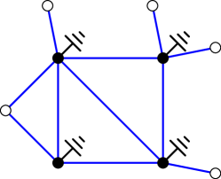
Fig. 1: A circuit with boundary nodes in white and interior nodes in black. Each interior node is connected to the ground, i.e. a single node with constant zero potential. The edges in blue correspond to a conductivity $\gamma$ and the edges in black to a Schrödinger potential $q$.

1.1 Applications

The problem of finding the conductivities in a graph arises in applications such as geophysical exploration [22] and medical imaging in a modality called electrical impedance tomography or EIT, for a review see [8]. The methods described in [8] are limited to 2D setups and real conductivities because they rely on results for the discrete inverse conductivity problem on graphs that were only known to hold for positive conductivities and for planar graphs. However, data from EIT is usually not static, and is usually taken for different frequencies because admittivity can help distinguish between different types of tissue (see e.g. the reviews [11, 7]). With the results presented here, we expect that the methods in [8] can be generalized to handling 3D setups, complex conductivities (admittivities) and the Schrödinger problem. As far as the continuum Schrödinger problem is concerned, some of the techniques in [8] are used in the forthcoming [9] to design a numerical method for solving the two-dimension Schrödinger problem in the (real) absorptive case which arises in e.g. diffuse optical tomography (see e.g. the review [6]).

1.2 Contents

We start in §2 by giving a review of available uniqueness results for inverse problems on graphs. Then in §3 we explain the parallels between our method and the complex geometric optics approach (in the continuum). This section is self-contained and its purpose is to motivate our approach. The forward and inverse discrete problems that we consider are defined in §4. The uniqueness result for the conductivity problem is in §5 and for the Schrödinger problem in §6. Numerical experiments, including a statistical study of graphs where either of these inverse problems can be solved are in §7. Interestingly, this study reveals that graphs on which the Schrödinger problem is solvable are much more common than graphs where the conductivity problem is solvable. We conclude with a discussion in §8. Because of their similarity to their conductivity problem analogues, we defer the proof of some results for the Schrödinger problem to Appendix A.

2 Related work

We review uniqueness results for the discrete inverse conductivity problem (§2.1), for the discrete inverse Schrödinger problem (§2.2) and finally some results on infinite lattices (§2.3).

2.1 Discrete inverse conductivity problem

The first uniqueness result for the discrete inverse conductivity problem that we are aware of is the constructive algorithm of Curtis and Morrow [20] to find a positive real conductivity in a rectangular graph. Then Curtis, Mooers and Morrow [18] gave a constructive algorithm to find the positive real conductivity in certain circular planar networks. This result was generalized independently by Colin de Verdière [15] and by Curtis, Ingerman and Morrow [19] to encompass positive real conductivities on circular planar graphs, i.e. all the graphs that can be embedded in a plane without edge crossings and for which the boundary (or accessible) nodes lie on a circle. The condition for recoverability is a condition on the connectedness of the graph and does not depend on the conductivity (see also [17, 16, 21]).

Other results by Chung and Berenstein [14] and Chung [13] are not limited to circular planar graphs, but assume monotonicity and positive real conductivities. These results are discrete analogous of the uniqueness result of Alessandrini [1] for the continuum conductivity problem (see also [30, §4.3]). In a nutshell, the result of Chung [14] guarantees that if two conductivities $\gamma_{1}\leq\gamma_{2}$ (the inequality being componentwise) agree in a neighborhood of the boundary nodes and one measurement of the potential and the corresponding current at the boundary is identical for both conductivities then $\gamma_{1}=\gamma_{2}$. The result [13] is an extension to other kinds of measurements.

We point also to the work by Lam and Pylyavskyy [32], which uses combinatorics to study networks that can be embedded in a cylinder (i.e. the nodes and edges lie on the cylinder’s surface with no edges crossing) and with boundary nodes at the two ends of the cylinder. They show that positive real conductivities cannot be uniquely determined from boundary data.

To our knowledge, our uniqueness result is the first that deals with complex conductivities and that is not limited to circular planar graphs. However our result is weaker than that in [15, 19] in the sense that we do not show uniqueness for all conductivities with positive real part, but we do show that the set of pairs of conductivities $\gamma_{1},\gamma_{2}$ that we cannot tell apart from boundary data is a set of measure zero.

2.2 Discrete inverse Schrödinger problem

The inverse Schrödinger problem on circular planar graphs has been studied by Araúz, Carmona and Encinas [3, 5, 4], and they also give conditions for which real Schrödinger potentials in a certain class (that makes them essentially equivalent to conductivities) can be determined from boundary data. Although our result is stronger in the sense that we allow for complex Schrödinger potentials and topologies that are not necessarily planar, our result is also weaker in the sense that we only have uniqueness up to a zero measure set of pairs of Schrödinger potentials $q_{1},q_{2}$ that are indistinguishable from boundary data.

2.3 Infinite lattices

We also note that there are related uniqueness results for infinite graphs (i.e. lattices) for both the inverse Schrödinger problem [33, 31, 2] and conductivity problem [24]. The latter being perhaps the closest to our results because it uses the complex geometric optics approach.

3 Relation with the complex geometric optics approach

We give here a brief summary of the uniqueness proof for the inverse Schrödinger problem by Sylvester and Uhlmann [36]. The intention of this summary is not to be complete or general, but to highlight the steps in the proof that have a discrete analogue in our argument. For reviews focussed on the complex geometric optics (CGO) approach for the inverse conductivity problem see e.g. [38, 35], for other inverse problems see e.g. [37]. Finally note that this is the only section where we use functions defined on a continuum, elsewhere functions are defined on a finite sets. Hence the notation is exclusive of this section.

3.1 The continuum inverse Schrödinger problem

Let $\Omega\subset\mathbb{R}^{d}$ be a domain with smooth boundary $\partial\Omega$ in dimension $d\geq 3$ and let $q\in L^{2}(\Omega)$ be a, possibly complex valued, function that we shall call Schrödinger potential. The Dirichlet problem for the Schrödinger equation is given the Dirichlet data $f\in H^{1/2}(\partial\Omega)$, find $u\in H^{1}(\Omega)$ such that

$$-\Delta u+qu=0~{}\text{in $\Omega$},~{}\text{and}~{}u=f~{}\text{on $\partial\Omega$}.$$ (1)

The Dirichlet to Neumann map is the linear mapping $\Lambda_{q}:H^{1/2}(\partial\Omega)\to H^{-1/2}(\partial\Omega)$ defined for $f\in H^{1/2}(\partial\Omega)$ by

$$\Lambda_{q}f=n\cdot\nabla u,$$ (2)

where $u$ solves (1) with Dirichlet boundary condition $f$ and $n$ is the unit normal to $\partial\Omega$ pointing outwards. We assume here that the Schrödinger potential $q$ is such that the Dirichlet problem (1) admits a unique solution for all boundary excitations $f\in H^{1/2}(\partial\Omega)$. The inverse Schrödinger problem is to find $q$ from the Dirichlet to Neumann map $\Lambda_{q}$.

3.2 An interior identity

The first step in the uniqueness proof of Sylvester and Uhlmann [36] for the Schrödinger inverse problem is to show an identity that relates a difference in boundary data to a difference in Schrödinger potentials times products of solutions to the Dirichlet problem:

$$\int_{\partial\Omega}(\Lambda_{q_{1}}-\Lambda_{q_{2}})(f_{1})f_{2}dS=\int_{\Omega}(q_{1}-q_{2})u_{1}u_{2}dx,$$ (3)

where $u_{j}$ solves the Dirichlet problem (1) with boundary data $f_{j}\in H^{1/2}(\partial\Omega)$, for $j=1,2$.

3.3 Density of products of solutions

The second step is to prove that products of solutions to the Dirichlet problem (1) are dense in some appropriate space, say $L^{2}(\Omega)$. If this were true and we had two Schrödinger potentials $q_{1}$ and $q_{2}$ for which $\Lambda_{q_{1}}=\Lambda_{q_{2}}$ we could use (3) to conclude that $\overline{q}_{1}-\overline{q}_{2}$ is in the orthogonal of a set that is dense in $L^{2}(\Omega)$. Therefore we get $q_{1}=q_{2}$ and uniqueness.

Calderón [10] proved that for the harmonic case ($q=0$) there is a family of complex exponential harmonic functions (hence the CGO name) such that for any $\xi\in\mathbb{R}^{d}$, one can pick two members $v_{1}$, $v_{2}$ in the family so that $v_{1}v_{2}=e^{ix\cdot\xi}$. Since $\xi$ is arbitrary, this is of course dense in $L^{2}(\Omega)$ by the Fourier transform. Crucially these members can be chosen with arbitrarily high frequencies. Since (1) is the Laplacian plus a lower order term, $v_{1}$ and $v_{2}$ plus appropriate corrections solve (1), and these corrections vanish in the high frequency limit. Hence high frequency asymptotic estimates show that if products of solutions to the Dirichlet problem with $q=0$ are dense in $L^{2}(\Omega)$, then products of solutions for any other $q$ are dense in $L^{2}(\Omega)$.

3.4 Parallels with the discrete setting

In a finite graph we work with functions defined on finite sets, so we do not have such high frequency asymptotics. The concept that replaces this is that of analytic continuation for functions of several complex variables (see e.g. [28]). Also in finite dimensions, saying that a family of vectors is dense in a space, simply means that the family spans the space.

4 The discrete Schrödinger and conductivity problems

We start in §4.1 with some preliminaries, then in §4.2 we define the weighted graph Laplacian. In §4.3 we give sufficient conditions on the conductivity and the Schrödinger potential for the Dirichlet problem to have a unique solution no matter what the prescribed value at the boundary nodes is. In §4.4 we formulate the inverse Schrödinger and conductivity problems. Then in §4.5 we give a discrete analogue to the Green identities.

4.1 Preliminaries

We consider graphs $\mathcal{G}=(V,E)$, where $V$ is a finite vertex set and $E\subset\{\{i,j\}~{}|~{}i,j\in V,~{}i\neq j\}$ is the edge set. The vertex set $V$ is partitioned into boundary nodes $B$ and interior nodes $I$. We use the set theory notation for functions, e.g. $f\in\mathbb{C}^{V}$ is a function $f:V\to\mathbb{C}$. Upon fixing an ordering of the vertices, $f$ can be identified to a vector in $\mathbb{C}^{|V|}$, that in a slight abuse of notation is also denoted by $f$. In the same way, we identify a linear operator $A:\mathbb{C}^{X}\to\mathbb{C}^{Y}$, where $X$ and $Y$ are finite sets (e.g. $X=E$ and $Y=V$), to a $|X|\times|Y|$ complex matrix which is also denoted by $A$.

4.2 The weighted graph Laplacian

The discrete gradient is the linear map $\nabla:\mathbb{C}^{V}\to\mathbb{C}^{E}$ such that

$$(\nabla u)(\{i,j\})=u(i)-u(j),~{}\mbox{for $u\in\mathbb{C}^{V}$ and $\{i,j\}\in E$.}$$ (4)

This definition depends on the ordering of vertices for an edge, but as long as it is fixed once and for all it is inessential to the following discussion.

Given a discrete conductivity $\gamma\in\mathbb{C}^{E}$, the weighted graph Laplacian $L_{\gamma}:\mathbb{C}^{V}\to\mathbb{C}^{V}$ by (see e.g. [12])

$$L_{\gamma}u=\nabla^{*}[\gamma\odot(\nabla u)]=\sum_{\{i,j\}\in E}\gamma(\{i,j\})(u(i)-u(j)),~{}\mbox{for $u\in\mathbb{C}^{V}$.}$$ (5)

Here $\nabla^{*}:\mathbb{C}^{E}\to\mathbb{C}^{V}$ is the adjoint of $\nabla$. Since the entries of $\nabla$ are real, we have $\nabla^{*}=\nabla^{T}$. By $u\odot v$ we mean the Hadamard product of two vectors, e.g. if $u,v\in\mathbb{C}^{E}$, $(u\odot v)(e)=u(e)v(e)$ for all $e\in E$. In matrix notation we have $L_{\gamma}=\nabla^{*}\mathop{\operator@font diag}\nolimits(\gamma)\nabla$.

4.3 The Dirichlet problem

For given $\gamma\in\mathbb{C}^{E}$ and $q\in\mathbb{C}^{I}$, the Dirichlet problem for $\gamma,q$ consists of finding the interior values $u_{I}\in\mathbb{C}^{I}$ from the boundary values $u_{B}\in\mathbb{C}^{B}$ such that

$$(L_{\gamma})_{IB}u_{B}+(L_{\gamma})_{II}u_{I}+q\odot u_{I}=0.$$ (6)

Here $(L_{\gamma})_{IB}$ means we restrict the rows of the Laplacian $L_{\gamma}$ to the index set $I$ and the columns to the index set $B$. A solution $u\in\mathbb{C}^{V}$ to the Dirichlet problem for $\gamma,q$ is said to be $\gamma,q$ harmonic. We say the Dirichlet problem for $\gamma,q$ is well-posed when the matrix $(L_{\gamma})_{II}+\mathop{\operator@font diag}\nolimits(q)$ is invertible. This means that the interior values $u_{I}\in\mathbb{C}^{I}$ are uniquely determined by the boundary values $u_{B}\in\mathbb{C}^{B}$. The following theorem gives conditions guaranteeing the $\gamma,q$ Dirichlet problem is well-posed. To write these conditions concisely, we denote by $\mathbb{C}_{\zeta}\equiv\{z\in\mathbb{C}~{}|~{}\mbox{Re}\,z>\zeta\}$ the open region to the right of the line $\mbox{Re}\,z=\zeta$ in the complex plane, where $\zeta\in\mathbb{R}$. In what follows it is convenient to consider the subgraph $\mathcal{G}_{I}=(I,E_{I})$ of $\mathcal{G}$ restricted to the interior nodes and with edge set

$$E_{I}\equiv\{\{i,j\}\in E~{}|~{}i,j\in I\}.$$ (7)

Theorem 1.

Assuming $\mathcal{G}$ and $\mathcal{G}_{I}$ are connected graphs, for all $\gamma\in\mathbb{C}_{0}^{E}$ there is a real number $\zeta<0$ such that the Dirichlet problem for $\gamma,q$ is well-posed for $q\in\mathbb{C}_{\zeta}^{I}$.

We call restricted Laplacian, the Laplacian $L_{\gamma_{I}}$ on $\mathcal{G}_{I}$ with weights $\gamma_{I}\equiv\gamma_{E_{I}}$. The restricted Laplacian and the $II$ block of the full Laplacian differ only by a diagonal term $\mu\in\mathbb{C}^{I}$, i.e.

$$(L_{\gamma})_{II}=L_{\gamma_{I}}+\mathop{\operator@font diag}\nolimits(\mu),$$ (8)

where the entries of $\mu$ are

$$\mu(j)=\sum_{i\in B,~{}\{i,j\}\in E}\gamma(\{i,j\}),~{}\text{for $j\in I$}.$$ (9)

If no entry of $\gamma$ is zero, the support of $\mu$ (i.e. the nodes $i$ for which $\mu(i)$ is non-zero) consists of the interior nodes that are connected by an edge to the boundary nodes, i.e. the nodes in the set

$$J=\{i\in I~{}|~{}\{i,j\}\in E~{}\text{for some $j\in B$}\}.$$ (10)

Proof of theorem 1.

Since $\gamma$ and $q$ are complex it is convenient to introduce the notation $\gamma=\gamma^{\prime}+i\gamma^{\prime\prime}$, where $\gamma^{\prime}\equiv\mbox{Re}\,\gamma$ and $\gamma^{\prime\prime}\equiv\mbox{Im}\,\gamma$ and similarly for $q$ and $\mu$ (as defined in (9)). We show that under the hypothesis of the theorem, the matrix $(L_{\gamma})_{II}+\mathop{\operator@font diag}\nolimits(q)$ is invertible. We do this by showing that the field of values (see e.g. [29]) of $(L_{\gamma})_{II}+\mathop{\operator@font diag}\nolimits(q)$, i.e. the region $W$ of the complex plane defined by

$$W\equiv\left\{{u^{*}[(L_{\gamma})_{II}+\mathop{\operator@font diag}\nolimits(q)]u~{}|~{}u\in\mathbb{C}^{I}~{}\text{with}~{}\|u\|^{2}=1}\right\},$$ (11)

is contained in $\mathbb{C}_{0}$. Since the spectrum is contained in the field of values of a matrix, this would mean that $0$ cannot be an eigenvalue of $(L_{\gamma})_{II}+\mathop{\operator@font diag}\nolimits(q)$, which is then invertible. The proof is divided in three steps.

Step 1. $\mbox{Re}\,(L_{\gamma})_{II}$ is Hermitian positive definite. Indeed we have

$$\mbox{Re}\,(L_{\gamma})_{II}=L_{\gamma^{\prime}_{I}}+\mathop{\operator@font diag}\nolimits(\mu^{\prime}).$$

Since $\gamma\in\mathbb{C}_{0}^{E}$, we clearly have $\gamma^{\prime}_{I}>0$, $\mu^{\prime}_{J}>0$ and $\mu^{\prime}_{I-J}=0$. Since the graph $\mathcal{G}_{I}$ is connected, the restricted Laplacian $L_{\gamma^{\prime}_{I}}$ must be Hermitian positive semidefinite with a one-dimensional nullspace spanned by the constant vector $[1,\ldots,1]^{T}\in\mathbb{C}^{I}$ (see e.g. [12] or [16]). Hence we have $u^{*}[L_{\gamma^{\prime}_{I}}+\mathop{\operator@font diag}\nolimits(\mu^{\prime})]u\geq 0$ for all $u\in\mathbb{C}^{I}$. Moreover if $u^{*}[L_{\gamma^{\prime}_{I}}+\mathop{\operator@font diag}\nolimits(\mu^{\prime})]u=0$, then $u=[a,\ldots,a]^{T}\in\mathbb{C}^{I}$ for some $a\in\mathbb{C}$. But then we must also have

$$0=|a|^{2}[1,\ldots,1]\mathop{\operator@font diag}\nolimits(\mu^{\prime})[1,\ldots,1]^{T}=|a|^{2}\sum_{j\in J}\mu^{\prime}(j).$$

Since $\mu^{\prime}_{J}>0$, the sum above is positive. Thus $|a|^{2}=0$ and $u=0$, which proves the desired result.

Step 2. $\mbox{Re}\,[(L_{\gamma})_{II}+\mathop{\operator@font diag}\nolimits(q)]$ is positive definite, for all $q\in\mathbb{C}^{I}$ with $q^{\prime}>\zeta_{\gamma}$, where

$$\zeta_{\gamma}\equiv-\lambda_{\min}((L_{\gamma^{\prime}})_{II}),$$ (12)

and $\lambda_{\min}(A)$ denotes the smallest eigenvalue (in magnitude) of a matrix $A$. By Step 1, $(L_{\gamma^{\prime}})_{II}$ is Hermitian positive definite so $\zeta_{\gamma}<0$. To show the desired result, notice that

$$\mbox{Re}\,[(L_{\gamma})_{II}+\mathop{\operator@font diag}\nolimits(q)]=(L_{\gamma^{\prime}})_{II}+\mathop{\operator@font diag}\nolimits(q^{\prime}),$$

is a Hermitian matrix, and for $u\in\mathbb{C}^{I}$ with $\|u\|^{2}=1$ its (real) Rayleigh quotient satisfies

$$u^{*}[(L_{\gamma^{\prime}})_{II}+\mathop{\operator@font diag}\nolimits(q^{\prime})]u \geq\lambda_{\min}((L_{\gamma^{\prime}})_{II})\|u\|^{2}+\sum_{i\in I}q^{\prime}(i)|u(i)|^{2}$$

$$>\lambda_{\min}((L_{\gamma^{\prime}})_{II})\|u\|^{2}+\zeta_{\gamma}\|u\|^{2}=0.$$

Step 3. The field of values $W$ is contained in $\mathbb{C}_{0}$. Let $u\in\mathbb{C}^{I}$ with $\|u\|^{2}=1$. Then we can write

$$u^{*}[(L_{\gamma})_{II}+\mathop{\operator@font diag}\nolimits(q)]u=u^{*}\mbox{Re}\,[(L_{\gamma})_{II}+\mathop{\operator@font diag}\nolimits(q)]u+iu^{*}\mbox{Im}\,[(L_{\gamma})_{II}+\mathop{\operator@font diag}\nolimits(q)]u.$$

Since $\mbox{Im}\,[(L_{\gamma})_{II}+\mathop{\operator@font diag}\nolimits(q)]=(L_{\gamma^{\prime\prime}})_{II}+\mathop{\operator@font diag}\nolimits(q^{\prime\prime})$ is Hermitian, we clearly have that $u^{*}\mbox{Im}\,[(L_{\gamma})_{II}+\mathop{\operator@font diag}\nolimits(q)]u\in\mathbb{R}$ and

$$\mbox{Re}\,(u^{*}[(L_{\gamma})_{II}+\mathop{\operator@font diag}\nolimits(q)]u)=u^{*}\mbox{Re}\,[(L_{\gamma})_{II}+\mathop{\operator@font diag}\nolimits(q)]u>0,$$

by the result of Step 2. Thus any point in $W$ must have positive real part. ∎

4.4 The inverse Schrödinger and conductivity problems

Provided the Dirichlet problem for $\gamma,q$ is well-posed, we can define the Dirichlet to Neumann map $\Lambda_{\gamma,q}:\mathbb{C}^{B}\to\mathbb{C}^{B}$ by the linear operator

$$\Lambda_{\gamma,q}u_{B}=(L_{\gamma})_{BB}u_{B}+(L_{\gamma})_{BI}u_{I},$$ (13)

where $u_{B}\in\mathbb{C}^{B}$ and $u_{I}\in\mathbb{C}^{I}$ is obtained from $u_{B}$ by solving (6). The Dirichlet to Neumann map can be written as the Schur complement of the block $(L_{\gamma})_{II}+\mathop{\operator@font diag}\nolimits(q)$ in the matrix

$$\begin{bmatrix}(L_{\gamma})_{BB}&(L_{\gamma})_{BI}\\ (L_{\gamma})_{IB}&(L_{\gamma})_{II}+\mathop{\operator@font diag}\nolimits(q)\end{bmatrix},$$ (14)

in other words:

$$\Lambda_{\gamma,q}=(L_{\gamma})_{BB}-(L_{\gamma})_{BI}[(L_{\gamma})_{II}+\mathop{\operator@font diag}\nolimits(q)]^{-1}(L_{\gamma})_{IB}.$$ (15)

The inverse conductivity problem is to find $\gamma\in\mathbb{C}^{E}$ from the Dirichlet to Neumann map $\Lambda_{\gamma,0}$, assuming the graph $\mathcal{G}=(V,E)$ and the boundary nodes $B$ are known.

The inverse Schrödinger problem is to find $q\in\mathbb{C}^{I}$ from the Dirichlet to Neumann map $\Lambda_{\gamma,q}$, assuming the graph $\mathcal{G}=(V,E)$, the boundary nodes $B$, and the conductivity $\gamma$ are known.

4.5 A discrete Green identity

Here is a discrete analogue of one of the Green identities that relates a sum over boundary nodes to a sum over all the nodes.

Lemma 2 (Green identity).

Let $\gamma$ and $q$ be such that the $\gamma,q$ Dirichlet problem is well-posed. Let $u,v\in\mathbb{C}^{V}$, with $v$ being $\gamma,q$ harmonic. Then we have the following:

$$u_{B}^{T}\Lambda_{\gamma,q}v_{B}=u^{T}L_{\gamma}v+u_{I}^{T}\mathop{\operator@font diag}\nolimits(q)v_{I}.$$ (16)

Proof.

The right hand side can be written as

$$u^{T}L_{\gamma}v+u_{I}^{T}\mathop{\operator@font diag}\nolimits(q)v_{I}=u_{B}^{T}(L_{\gamma}v)_{B}+u_{I}^{T}(L_{\gamma}v+\widetilde{q}\odot v)_{I}=u_{B}^{T}(L_{\gamma}v)_{B},$$ (17)

where $\widetilde{q}_{B}\equiv 0$ and $\widetilde{q}_{I}\equiv q$. The last equality comes from $v$ being a solution to the Dirichlet problem (6) for $\gamma,q$. The desired result follows from the definition of the Dirichlet to Neumann map (13) by noticing that

$$(L_{\gamma}v)_{B}=(L_{\gamma})_{BB}v_{B}+(L_{\gamma})_{BI}v_{I}=\Lambda_{\gamma,q}v_{B},$$

when $v$ is $\gamma,q$ harmonic. ∎

5 Solvability for the inverse conductivity problem

We now show a uniqueness result for the inverse conductivity problem. We start by showing an identity similar to the one used in [10, 36] that relates a difference in boundary data to a difference in conductivities (§5.1). This identity relates the uniqueness question to studying the space spanned by products of (discrete) gradients of solutions (§5.2). The result has applications to Newton’s method (§5.3) and can be interpreted probabilistically (§5.4). The main uniqueness result is proved in §5.5.

5.1 An interior identity

The following lemma relates the difference in the boundary data for two conductivities to the conductivity difference. This identity is a discrete analogue to the one appearing in [36].

Lemma 3 (Interior identity for conductivities).

Let $\gamma_{1},\gamma_{2}\in\mathbb{C}_{0}^{E}$, $u$ be $\gamma_{1},0$ harmonic and $v$ be $\gamma_{2},0$ harmonic. Then the following identity holds

$$u_{B}^{T}(\Lambda_{\gamma_{1},0}-\Lambda_{\gamma_{2},0})v_{B}=(\gamma_{1}-\gamma_{2})^{T}\left[{(\nabla u)\odot(\nabla v)}\right].$$ (18)

Proof.

By using lemma 2 twice we get:

$$u_{B}^{T}\Lambda_{\gamma_{1},0}v_{B}=u^{T}L_{\gamma_{1},0}v,~{}\text{and}~{}u_{B}^{T}\Lambda_{\gamma_{2},0}v_{B}=u^{T}L_{\gamma_{2},0}v.$$

Subtracting the second equation from the first we get

$$u_{B}^{T}(\Lambda_{\gamma_{1},0}-\Lambda_{\gamma_{2},0})v_{B}=u^{T}(L_{\gamma_{1},0}-L_{\gamma_{2},0})v=u^{T}\nabla^{T}\mathop{\operator@font diag}\nolimits(\gamma_{1}-\gamma_{2})\nabla v,$$

which gives the desired result. ∎

5.2 Uniqueness almost everywhere

Inspired by the complex geometric optics method [10, 36], we would like to study the subspaces of $\mathbb{C}^{E}$

$$P(\gamma_{1},\gamma_{2})\equiv\operatorname{span}\left\{{(\nabla u)\odot(\nabla v)~{}|~{}\text{$u$ is $\gamma_{1},0$ harmonic and $v$ is $\gamma_{2},0$ harmonic}}\right\},$$ (19)

for conductivities $\gamma_{1},\gamma_{2}\in\mathbb{C}_{0}^{E}$. To see why this subspace is important, assume there are two conductivities $\gamma_{1},\gamma_{2}$ with the same boundary data, i.e. $\Lambda_{\gamma_{1},0}=\Lambda_{\gamma_{2},0}$, then lemma 3 implies that $\overline{\gamma}_{1}-\overline{\gamma}_{2}\in P(\gamma_{1},\gamma_{2})^{\perp}$. Hence if we are so fortunate to have $P(\gamma_{1},\gamma_{2})=\mathbb{C}^{E}$ we would conclude that $\gamma_{1}=\gamma_{2}$.

Theorem 4 (Uniqueness almost everywhere for conductivities).

If there is $\rho_{1},\rho_{2}\in\mathbb{C}_{0}^{E}$ such that $P(\rho_{1},\rho_{2})=\mathbb{C}^{E}$, then $P(\gamma_{1},\gamma_{2})=\mathbb{C}^{E}$ for almost all $(\gamma_{1},\gamma_{2})\in\mathbb{C}_{0}^{E}\times\mathbb{C}_{0}^{E}$.

The condition $P(\gamma_{1},\gamma_{2})=\mathbb{C}^{E}$ implies that $\Lambda_{\gamma_{1},0}\neq\Lambda_{\gamma_{2},0}$ whenever $\gamma_{1}\neq\gamma_{2}$, i.e. wherever this condition holds we can distinguish two conductivities from their DtN maps. The conclusion of Theorem 4 says that conductivities are distinguishable except for a zero measure set $Z$ of $(\gamma_{1},\gamma_{2})$ for which $P(\gamma_{1},\gamma_{2})\neq\mathbb{C}^{E}$. What happens in $Z$ is not so clear cut. The set $Z$ contains all $(\gamma_{1},\gamma_{2})$ for which $\gamma_{1}\neq\gamma_{2}$ but $\Lambda_{\gamma_{1},0}=\Lambda_{\gamma_{2},0}$. However $Z$ may also contain other $(\gamma_{1},\gamma_{2})$ for which $\Lambda_{\gamma_{1},0}\neq\Lambda_{\gamma_{2},0}$. Hence, theorem 4 guarantees that the set $C\subset Z$ of $(\gamma_{1},\gamma_{2})$ for which $\Lambda_{\gamma_{1},0}=\Lambda_{\gamma_{2},0}$ but $\gamma_{1}\neq\gamma_{2}$ is of measure zero in $\mathbb{C}_{0}^{E}\times\mathbb{C}_{0}^{E}$. We can refine the conclusion of theorem 4 by considering equivalence classes of conductivities for the equivalence relation $\Lambda_{\gamma_{1},0}=\Lambda_{\gamma_{2},0}$.

Corollary 5.

If there is $\rho_{1},\rho_{2}\in\mathbb{C}_{0}^{E}$ such that $P(\rho_{1},\rho_{2})=\mathbb{C}^{E}$, then any equivalence class of conductivities in $\mathbb{C}_{0}^{E}$ for the equivalence relation $\Lambda_{\gamma_{1},0}=\Lambda_{\gamma_{2},0}$ must be of measure zero in $\mathbb{C}_{0}^{E}$.

Proof.

Since the hypothesis of theorem 4 holds, the set $Z$ of $(\gamma_{1},\gamma_{2})$ for which $P(\gamma_{1},\gamma_{2})\neq\mathbb{C}^{E}$ is of measure zero. Let $M$ be an equivalence class of conductivities that are indistinguishable from their DtN maps. With $\mathop{\operator@font diag}\nolimits(M\times M)=\{(\gamma,\gamma)|\gamma\in M\}$, we clearly have $M\times M-\mathop{\operator@font diag}\nolimits(M\times M)\subset Z$. Hence $M\times M-\mathop{\operator@font diag}\nolimits(M\times M)$ is of measure zero and so is $M\times M$. Therefore $M$ is of measure zero. ∎

For another point of view, we consider the linearization of the boundary data $\Lambda_{\gamma,0}$ with respect to changes in the conductivity $\gamma$.

Lemma 6 (Linearization for conductivities).

Let $\gamma\in\mathbb{C}_{0}^{E}$. Then for sufficiently small $\delta\gamma\in\mathbb{C}^{E}$,

$$u_{B}^{T}\Lambda_{\gamma+\delta\gamma,0}v_{B}=u_{B}^{T}\Lambda_{\gamma,0}v_{B}+(\delta\gamma)^{T}[(\nabla u)\odot(\nabla v)]+o(\delta\gamma),$$ (20)

where $u=(u_{B},u_{I})$ and $v=(v_{B},v_{I})$ are $\gamma,0$ harmonic.

Proof.

Use the interior identity (18) with $\gamma_{1}=\gamma+\epsilon\delta\gamma$ and $\gamma_{2}=\gamma$, divide by $\epsilon$ and take the limit as $\epsilon\to 0$. ∎

The mapping $\gamma\to\Lambda_{\gamma,0}$ is thus Fréchet differentiable and it’s Jacobian $D_{\gamma}\Lambda_{\gamma,0}:\mathbb{C}^{E}\to\mathbb{C}^{B\times B}$ about $\gamma$ is

$$D_{\gamma}\Lambda_{\gamma,0}\delta\gamma=L_{BI}L_{II}^{-1}\nabla^{T}\mathop{\operator@font diag}\nolimits(\delta\gamma)\nabla L_{II}^{-1}L_{IB},$$ (21)

for $\delta\gamma\in\mathbb{C}^{E}$ and where we omitted the subscript $\gamma$ in the weighted graph Laplacian $L_{\gamma}$. We say the linearized problem is solvable at $\gamma$, when the Jacobian about $\gamma$ is injective, i.e. the nullspace $\operatorname{\mathcal{N}}(D_{\gamma}\Lambda_{\gamma,0})=\{0\}$. Solvability of the linearized inverse problem about $\gamma$ is of course equivalent to the range $\operatorname{\mathcal{R}}(D_{\gamma}\Lambda_{\gamma,0}^{*})=\mathbb{C}^{E}=P(\gamma,\gamma)$, where the last equality comes from lemma 6 and the definition of the Jacobian. Hence by taking $\rho_{1}=\rho_{2}$ in theorem 4 we immediately get the following corollary.

Corollary 7.

If the linearized problem is solvable about some $\rho\in\mathbb{C}_{0}^{E}$ then $\Lambda_{\gamma_{1},0}=\Lambda_{\gamma_{2},0}$ implies $\gamma_{1}=\gamma_{2}$, for almost all $(\gamma_{1},\gamma_{2})\in\mathbb{C}_{0}^{E}\times\mathbb{C}_{0}^{E}$.

The same proof technique for Theorem 17 can be used to prove the following.

Corollary 8.

If the linearized problem is solvable about some $\rho\in\mathbb{C}_{0}^{E}$ then it is solvable for almost all $\gamma\in\mathbb{C}_{0}^{E}$.

A consequence of Corollary 8 is that the solvability of the linearized inverse problem does not depend on the actual conductivity (except for a set of measure zero). This is without any topological assumptions on the graph. This fact was already known for circular planar graphs [18, 19].

Corollary 8 suggests a simple test for checking whether the conductivity problem is solvable in a graph. All we need to do is check whether the Jacobian about some conductivity, say $\gamma=1$ (the constant conductivity equal to one), has a trivial nullspace. Of course, this may give a false negative if $P(\gamma,\gamma)=\mathbb{C}^{E}$ for almost all $\gamma\in\mathbb{C}_{0}^{E}$ but $P(1,1)\neq\mathbb{C}^{E}$. However we have verified numerically that this is unlikely to happen.

The following corollary shows that if we start at a conductivity for which the linearized problem is solvable and go in any direction we may encounter only finitely many conductivities that have the same DtN map or where the problem is not solvable. The proof of this result requires notation introduced for the proof of theorem 4 and is thus presented in §5.5.

Corollary 9.

If the linearized problem is solvable at $\gamma\in\mathbb{C}^{E}_{0}$ then along any direction $\delta\gamma\in\mathbb{C}^{E}$ there are at most finitely many $t\in\mathbb{C}$ with $\mbox{Re}\,(\gamma+t\delta\gamma)>0$ for which

• the linearized problem is not solvable at $\gamma+t\delta\gamma$.

• $\gamma$ and $\gamma+t\delta\gamma$ may have the same DtN map (i.e. $P(\gamma,\gamma+t\delta\gamma)\neq\mathbb{C}^{E}$).

Remark 10.

As appears later in §5.5, the proof of theorem 4 hinges on complex analyticity. If we use real analyticity instead, we can get results analogous to theorem 4 and corollaries 5, 7, 8 and 9, but where $\mathbb{C}$ is replaced by $\mathbb{R}$. The set $\mathbb{R}_{0}^{E}$ is then the (open) positive orthant of $\mathbb{R}^{E}$.

5.3 Application to Newton’s method

Corollary 9 is useful to show that the systems in Newton’s method applied to finding the conductors in a graph are very likely to admit a unique solution (if only a finite number of iterations are carried out). Newton’s method applied to finding $\gamma$ from $\Lambda_{\gamma,0}$ takes the form (see e.g. [34])

Newton’s method
$\gamma^{(0)}=$ given
for $k=0,1,2,\ldots$
	Find step $\delta\gamma^{(k)}$ s.t. $D_{\gamma}\Lambda_{\gamma^{(k)},0}\delta\gamma^{(k)}=\Lambda_{\gamma^{(k)},0}-\Lambda_{\gamma,0}$
	Choose step length $t_{k}>0$
	Update $\gamma^{(k+1)}=\gamma^{(k)}+t_{k}\delta\gamma^{(k)}$

where the $\gamma^{(k)}$ are the iterates that hopefully converge to $\gamma$ and $t_{k}>0$ is a parameter used to adjust the step length and ensure feasibility ($\mbox{Re}\,\gamma^{(k)}>0$). If the linearized problem about the $k-$th iterate $\gamma^{(k)}$ is solvable, then the linear system we need to solve to find the $k-$th step admits a unique solution $\delta\gamma^{(k)}$. Moreover the linearized problem is solvable almost everywhere (by corollary 7), so we can expect that the linearized problem is solvable at the next iterate $\gamma^{(k)}$. In fact corollary 9 guarantees that up to finitely many exceptions, all choices of the next iterate $\gamma^{(k+1)}$ are such that the linearized problem is solvable.

5.4 A probabilistic interpretation

From a probabilistic point of view, the conclusion of Theorem 4 means intuitively that if we choose two conductivities at random, there is zero probability that $P(\gamma_{1},\gamma_{2})\neq\mathbb{C}^{E}$. To see this consider an absolutely continuous (with respect to the Lebesgue measure) random vector $(\Gamma_{1},\Gamma_{2})\in\mathbb{C}^{E}_{0}\times\mathbb{C}_{0}^{E}$ with distribution $\mu$ and induced probability measure $\operatorname{\mathbb{P}}$. If the hypothesis of theorem 4 hold and $M\subset\mathbb{C}^{E}_{0}\times\mathbb{C}_{0}^{E}$ is a measurable set with $\operatorname{\mathbb{P}}\left[{(\Gamma_{1},\Gamma_{2})\in M}\right]>0$ then

$$\operatorname{\mathbb{P}}\left[{P(\Gamma_{1},\Gamma_{2})=\mathbb{C}^{E}~{}|~{}(\Gamma_{1},\Gamma_{2})\in M}\right]=1.$$ (22)

Indeed the conclusion of theorem 4 means that the set

$$Z=\left\{{(\Gamma_{1},\Gamma_{2})\in M~{}|~{}P(\Gamma_{1},\Gamma_{2})\neq\mathbb{C}^{E}}\right\}$$ (23)

is a set of measure zero and therefore by absolute continuity of $\mu$ we also have $\mu(Z)=0$. Moreover the set $Z$ contains all the pairs $(\gamma_{1},\gamma_{2})$ for which $\Lambda_{\gamma_{1}}=\Lambda_{\gamma_{2}}$ but $\gamma_{1}\neq\gamma_{2}$, i.e conductivities that are indistinguishable from boundary measurements. Hence we also have that the expectation

$$\operatorname{\mathbb{E}}\left[{\|\Lambda_{\Gamma_{1},0}-\Lambda_{\Gamma_{2},0}\|~{}|~{}(\Gamma_{1},\Gamma_{2})\in M}\right]=\int_{M}\|\Lambda_{\Gamma_{1},0}-\Lambda_{\Gamma_{2},0}\|~{}d\mu>0.$$ (24)

The conclusion of Corollary 8 means that if $\Gamma$ is an absolutely continuous random vector on $\mathbb{C}_{0}^{E}$, then on any measurable set $M\subset\mathbb{C}_{0}^{E}$ with $\operatorname{\mathbb{P}}\left[{\Gamma\in M}\right]>0$, we must have that

$$\operatorname{\mathbb{P}}\left[{D_{\gamma}\Lambda_{\Gamma,0}~{}\text{is injective}~{}|~{}\Gamma\in M}\right]=1.$$ (25)

We conclude this section by noting that uniqueness a.e. arises naturally in (finite dimensional) linear systems.

Example 11.

Another example of uniqueness a.e. is that of a matrix that has a non-trivial nullspace. Let $A\in\mathbb{C}^{m\times n}$, with $A\neq 0$ and $\operatorname{\mathcal{N}}(A)\neq\{0\}$. Then $\operatorname{\mathcal{N}}(A)$ is a subspace of $\mathbb{C}^{n}$ of dimension at most $n-1$, and as such is a set of Lebesgue measure zero in $\mathbb{C}^{n}$. Hence for almost all $(x_{1},x_{2})\in\mathbb{C}^{n}\times\mathbb{C}^{n}$, $Ax_{1}=Ax_{2}$ implies $x_{1}=x_{2}$.

5.5 Proof of uniqueness a.e. for conductivities

First we note that the product of solutions subspace is spanned by finitely many Dirichlet problem solutions.

Lemma 12.

Let $\gamma_{1},\gamma_{2}\in\mathbb{C}^{E}_{0}$. Let $u^{(i)}$ (resp. $v^{(i)}$) be $\gamma_{1},0$ (resp. $\gamma_{2},0$) harmonic with boundary data $u^{(i)}_{B}=v^{(i)}_{B}=e_{i}$, where $\{e_{i}\}_{i\in B}$ is the canonical basis of $\mathbb{C}^{B}$. Then the product of solutions subspace is such that

$$P(\gamma_{1},\gamma_{2})=\operatorname{span}\left\{{(\nabla u^{(i)})\odot(\nabla v^{(j)})}\right\}_{i,j\in B}.$$ (26)

Proof.

By definition of the product of solutions subspace, we must have

$$\operatorname{span}\left\{{(\nabla u^{(i)})\odot(\nabla v^{(j)})}\right\}_{i,j\in B}\subset P(\gamma_{1},\gamma_{2}).$$

Let $w\in P(\gamma_{1},\gamma_{2})$, then $w=(\nabla u)\odot(\nabla v)$, where $u$ is $\gamma_{1},0$ harmonic and $v$ is $\gamma_{2},0$ harmonic. Since the Dirichlet problems for $\gamma_{1},0$ and $\gamma_{2},0$ are well-posed, we have

$$u=\sum_{i\in B}u_{B}(i)u^{(i)}~{}\text{and}~{}v=\sum_{j\in B}v_{B}(j)v^{(j)}.$$

Hence $w$ can be written as a linear combination of the $(\nabla u^{(i)})\odot(\nabla v^{(j)})$ and we have the inclusion $P(\gamma_{1},\gamma_{2})\subset\operatorname{span}\left\{{(\nabla u^{(i)})\odot(\nabla v^{(j)})}\right\}_{i,j\in B}$, which gives the desired result. ∎

Another way to write the subspace $P(\gamma_{1},\gamma_{2})$ is as the range of a matrix, i.e.

$$P(\gamma_{1},\gamma_{2})=\operatorname{\mathcal{R}}(F(\gamma_{1},\gamma_{2})),$$ (27)

where the matrix $F(\gamma_{1},\gamma_{2})\in\mathbb{C}^{|E|\times|B|^{2}}$ is the matrix with columns being all possible Hadamard products between the columns of the matrices $\nabla U(\gamma_{1})$ and $\nabla U(\gamma_{2})$, where $U(\gamma)$ is the matrix with solutions corresponding to boundary data $e_{i}$, $i\in B$, that is

$$U(\gamma)=\begin{bmatrix}\mathbb{I}_{B}\\ ((L_{\gamma})_{II})^{-1}L_{IB}\end{bmatrix}.$$

where $\mathbb{I}_{B}$ is the $|B|\times|B|$ identity matrix. Concretely, the matrix $F(\gamma_{1},\gamma_{2})$ is given by

$$[F(\gamma_{1},\gamma_{2})]_{:,i+(j-1)|B|}=\left[{\nabla U(\gamma_{1})}\right]_{:,i}\odot\left[{\nabla U(\gamma_{2})}\right]_{:,j},~{}\text{for}~{}i,j=1,\ldots,|B|,$$ (28)

where the $i-$th column of a matrix $A$ is denoted by $A_{:,i}$.

We are interested in finding a way of characterizing whether the products of (gradients of) solutions span $\mathbb{C}^{E}$ or not. One way to do this is to look at the determinants

$$f_{\alpha}(\gamma_{1},\gamma_{2})=\det[F(\gamma_{1},\gamma_{2})]_{:,\alpha}$$ (29)

where the matrix $[F(\gamma_{1},\gamma_{2})]_{:,\alpha}$ is the $|E|\times|E|$ submatrix of $F(\gamma_{1},\gamma_{2})$ obtained by selecting the $|E|$ columns corresponding to the multi-index $\alpha\in\{1,\ldots,|B|^{2}\}^{|E|}$. Thus $P(\gamma_{1},\gamma_{2})=\mathbb{C}^{E}$ if and only if there is an $\alpha\in\{1,\ldots,|B|^{2}\}^{|E|}$ for which $f_{\alpha}(\gamma_{1},\gamma_{2})\neq 0$. When $|B|^{2}<|E|$, all such determinants are zero (since we must have have repeated columns). When $|B|^{2}\geq|E|$, it is enough to check the $\binom{|B|^{2}}{|E|}$ choices of columns $\alpha=(\alpha_{1},\ldots,\alpha_{|E|})$, with $1\leq\alpha_{1}<\ldots<\alpha_{|E|}\leq|B|^{2}$. This observation is summarized in the following lemma.

Lemma 13.

Let $\gamma_{1},\gamma_{2}\in\mathbb{C}_{0}^{E}$. The following statements are equivalent

• $P(\gamma_{1},\gamma_{2})=\mathbb{C}^{E}$

• $\mathop{\operator@font rank}\nolimits F(\gamma_{1},\gamma_{2})=|E|$

• $f_{\alpha}(\gamma_{1},\gamma_{2})\neq 0$ for some $\alpha\in\{1,\ldots,|B|^{2}\}^{|E|}$ with $1\leq\alpha_{1}<\ldots<\alpha_{|E|}\leq|B|^{2}$.

Remark 14.

Finding the rank of $F(\gamma_{1},\gamma_{2})$ by checking the determinants of all possible square submatrices with maximal dimensions is not very efficient and is notoriously inaccurate to calculate in floating point arithmetic. A better way would be to test whether the smallest singular value of $F(\gamma_{1},\gamma_{2})$ is close to zero, and this is what we have used in the numerics (§7). Nevertheless we use this determinantal characterization of rank in the proof of theorem 4 because it is an algebraic operation that preserves analyticity.

The notion of analyticity that we use here is that of analytic (or holomorphic) functions of several complex variables (see e.g. [28]). We recall that a function $f:\mathbb{C}^{n}\to\mathbb{C}$ is analytic on some open set $U\subset\mathbb{C}^{n}$ if for each $z_{0}\in U$, $f(z)$ can be expressed as a power series that converges on $U$, i.e.

$$f(z)=\sum_{\alpha\in{\rm Nature}^{n}}c_{\alpha}(z-z_{0})^{\alpha},$$

where for a multi-index $\alpha=(\alpha_{1},\ldots,\alpha_{n})\in{\rm Nature}^{n}$ we have for $z\in\mathbb{C}^{n}$ that $z^{\alpha}=z_{1}^{\alpha_{1}}\ldots z_{n}^{\alpha_{n}}$. In particular, rational functions of the form $A(z)/B(z)$, for two polynomials $A(z)$ and $B(z)$, are analytic on any connected open set where $B(z)\neq 0$. Hence we have the following.

Lemma 15.

The functions $f_{\alpha}:\mathbb{C}^{E}_{0}\times\mathbb{C}^{E}_{0}\to\mathbb{C}$ are analytic for any $\alpha\in\{0,\ldots,|B|^{2}\}^{|E|}$.

Proof.

Let $\gamma_{1},\gamma_{2}\in\mathbb{C}_{0}^{E}$. First note that the entries of the matrices $((L_{\gamma_{k}})_{II})^{-1}$, $k=1,2$, are complex analytic on $\gamma_{1}$ and $\gamma_{2}$ when $\gamma_{1},\gamma_{2}\in\mathbb{C}^{E}_{0}$. This is because the cofactor formula for the inverse guarantees that the entries of the matrices in question are rational functions in $\gamma_{1},\gamma_{2}$ which are analytic provided $\det((L_{\gamma_{k}})_{II})\neq 0$, $k=1,2$. As in the proof of theorem 1, the condition $\gamma_{1},\gamma_{2}\in\mathbb{C}^{E}_{0}$ ensures that $\det(L_{\gamma_{k}})_{II}\neq 0$, $k=1,2$. Since $F(\gamma_{1},\gamma_{2})$ is obtained from $\nabla((L_{\gamma_{k}})_{II})^{-1}(L_{\gamma})_{IB}$, $k=1,2$ by taking columnwise Hadamard products, each entry of $F(\gamma_{1},\gamma_{2})$ is also analytic on $\gamma_{1}$ and $\gamma_{2}$ when $\gamma_{1},\gamma_{2}\in\mathbb{C}^{E}_{0}$. Finally taking the determinant of a matrix with analytic entries is also analytic. ∎

We are now ready to prove the main result.

Proof of Theorem 4.

By lemma 13, the theorem hypothesis means that there is some multi-index $\beta\in\{1,\ldots,|B|^{2}\}^{|E|}$ such that

$$f_{\beta}(\rho_{1},\rho_{2})\neq 0,~{}\text{for some $\rho_{1},\rho_{2}\in\mathbb{C}^{|E|}_{0}$}.$$

Thus $f_{\beta}$ is not identically zero. In fact its zero set restricted to $\mathbb{C}^{|E|}_{0}\times\mathbb{C}^{|E|}_{0}$

$$Z(f_{\beta})=\left\{{(\gamma_{1},\gamma_{2})\in\mathbb{C}^{|E|}_{0}\times\mathbb{C}^{|E|}_{0}~{}|~{}f_{\beta}(\gamma_{1},\gamma_{2})=0}\right\},$$ (30)

must be a set of measure zero (see e.g. [28]), where we use the Lebesgue measure on $\mathbb{C}^{|E|}\times\mathbb{C}^{|E|}$. By lemma 13, the subset $S$ of $\mathbb{C}^{|E|}_{0}\times\mathbb{C}^{|E|}_{0}$ on which $P(\gamma_{1},\gamma_{2})\neq\mathbb{C}^{E}$ is

$$S=\bigcap_{\alpha\in\{1,\ldots,|B|^{2}\}^{|E|}}Z(f_{\alpha}).$$

Since $Z(f_{\beta})$ has measure zero, the set $S\subset Z(f_{\beta})$ must have measure zero as well by monotonicity of the Lebesgue measure. ∎

Using the notation in this section we get the following.

Proof of corollary 9.

We start by showing (i). If the linearized problem at $\gamma$ is solvable, then there is some multi-index $\beta$ for which $f_{\beta}(\gamma,\gamma)\neq 0$. The function $f^{(1)}:\mathbb{C}\to\mathbb{C}$ given by

$$f^{(1)}(t)=f_{\beta}(\gamma+t\delta\gamma,\gamma+t\delta\gamma)$$

is an analytic function of the single variable $t$ on the set

$$K=\{t\in\mathbb{C}~{}|~{}\mbox{Re}\,(\gamma+t\delta\gamma)>0\}.$$

The set $K$ is a finite intersection of open convex sets (open half planes) containing a neighborhood of the origin and is thus also open, convex and connected. Moreover, $f^{(1)}(t)$ is a rational function in $t$ with no poles in $K$ and thus it may have only finitely many $t\in K$ for which $f^{(1)}(t)=0$. Part (ii) follows similarly from considering the function $f^{(2)}:\mathbb{C}\to\mathbb{C}$ given by

$$f^{(2)}(t)=f_{\beta}(\gamma,\gamma+t\delta\gamma),$$

which is also a rational function in $t$ with no poles in $K$. ∎

6 Solvability for the inverse Schrödinger problem

The same technique can be used to study the solvability for the inverse Schrödinger problem. First we relate a difference in boundary data to a difference of Schrödinger potentials (§6.1). The appropriate products of solutions subspace is defined in §6.2. The proof of the uniqueness result is deferred to Appendix A.

6.1 An interior identity

Let us write a relation similar to the continuum relation in [36] that relates a difference in boundary data to a difference in Schrödinger potentials.

Lemma 16 (Interior identity for Schrödinger potentials).

Let $\gamma\in\mathbb{C}_{0}^{E}$ and $q_{1},q_{2}\in\mathbb{C}^{I}$ be such that the $\gamma,q_{1}$ and $\gamma,q_{2}$ Dirichlet problems are well-posed. Let $u$ be $\gamma,q_{1}$ harmonic and $v$ be $\gamma,q_{2}$ harmonic. Then we have the following identity

$$u_{B}^{T}(\Lambda_{\gamma,q_{1}}-\Lambda_{\gamma,q_{2}})v_{B}=u_{I}^{T}\mathop{\operator@font diag}\nolimits(q_{1}-q_{2})v_{I}=(q_{1}-q_{2})^{T}(u_{I}\odot v_{I}).$$ (31)

Proof.

The proof is very similar to the proof in the continuum [36]. Since $u$ is $\gamma,q_{1}$ harmonic, lemma 2 guarantees that

$$u_{B}^{T}\Lambda_{\gamma,q_{1}}v_{B}=u^{T}L_{\gamma}v+u_{I}^{T}\mathop{\operator@font diag}\nolimits(q_{1})v_{I}.$$ (32)

Since $v$ is $\gamma,q_{2}$ harmonic we also have

$$u_{B}^{T}\Lambda_{\gamma,q_{2}}v_{B}=u^{T}L_{\gamma}v+u_{I}^{T}\mathop{\operator@font diag}\nolimits(q_{2})v_{I}.$$ (33)

The desired result is obtained by subtracting (33) from (32). ∎

6.2 Uniqueness almost everywhere

As in the uniqueness proof for the continuum Schrödinger problem [36], we would like to study the subspaces of $\mathbb{C}^{I}$,

$$Q(q_{1},q_{2})\equiv\operatorname{span}\left\{{u_{I}\odot v_{I}~{}|~{}\text{$u$ is $\gamma,q_{1}$ harmonic and $v$ is $\gamma,q_{2}$ harmonic}}\right\},$$ (34)

for potentials $q_{1}$ and $q_{2}$ that ensure the corresponding Dirichlet problems are well-posed. If the two potentials $q_{1}$ and $q_{2}$ gave identical boundary data, i.e. $\Lambda_{\gamma,q_{1}}=\Lambda_{\gamma,q_{2}}$, then lemma 16 implies that $\overline{q}_{1}-\overline{q}_{2}\in Q(q_{1},q_{2})^{\perp}$. If in addition we had that $Q(q_{1},q_{2})=\mathbb{C}^{I}$ we could conclude that $q_{1}=q_{2}$, which gives uniqueness. The following theorem is very similar to the uniqueness theorem 4 for conductivities, but with Dirichlet well-posedness conditions that are slightly more complicated.

Theorem 17 (Uniqueness almost everywhere for Schrödinger potentials).

Let $\gamma\in\mathbb{C}_{0}^{E}$ and $\zeta=-\lambda_{\min}(\mbox{Re}\,(L_{\gamma})_{II})$. If $Q(p_{1},p_{2})=\mathbb{C}^{I}$ for some $p_{1},p_{2}\in\mathbb{C}^{I}_{\zeta}$, then $Q(q_{1},q_{2})=\mathbb{C}^{I}$ for almost all $(q_{1},q_{2})\in\mathbb{C}^{I}_{\zeta}\times\mathbb{C}^{I}_{\zeta}$.

Since the proof of theorem 17 is very similar to that of theorem 4, it is deferred to Appendix A. Clearly, if the hypothesis of the theorem holds, $\Lambda_{\gamma,q_{1}}=\Lambda_{\gamma,q_{2}}$ implies $q_{1}=q_{2}$, for all $(q_{1},q_{2})\in\mathbb{C}^{I}_{\zeta}\times\mathbb{C}^{I}_{\zeta}$, except for a set of Lebesgue measure zero in $\mathbb{C}^{I}_{\zeta}\times\mathbb{C}^{I}_{\zeta}$. The linearization of the boundary data $\Lambda_{\gamma,q}$ with respect to changes in the potential $q$ is as follows.

Lemma 18 (Linearization for Schrödinger potentials).

Assume the Dirichlet problem for $\gamma,q$ is well-posed, then for sufficiently small $\delta q\in\mathbb{C}^{I}$, and any $u_{B},v_{B}\in\mathbb{C}^{B}$,

$$u_{B}^{T}\Lambda_{\gamma,q+\delta q}v_{B}=u_{B}^{T}\Lambda_{\gamma,q}v_{B}+(\delta q)^{T}(u_{I}\odot v_{I})+o(\delta q),$$ (35)

where $u=(u_{B},u_{I})$ and $v=(v_{B},v_{I})$ are $\gamma,q$ harmonic.

Proof.

Use the interior identity (31) with $q_{1}=q+\epsilon\delta q$ and $q_{2}=q$, divide by $\epsilon$ and take the limit as $\epsilon\to 0$. ∎

The previous lemma shows that the mapping $q\to\Lambda_{\gamma,q}$ is Fréchet differentiable. The Jacobian $D_{q}\Lambda_{\gamma,q}:\mathbb{C}^{I}\to\mathbb{C}^{B\times B}$ of $\Lambda_{\gamma,q}$ about $q$ is

$$D_{q}\Lambda_{\gamma,q}\delta q=L_{BI}(L_{II}+\mathop{\operator@font diag}\nolimits(q))^{-1}\mathop{\operator@font diag}\nolimits(\delta q)(L_{II}+\mathop{\operator@font diag}\nolimits(q))^{-1}L_{IB},$$ (36)

where $\delta q\in\mathbb{C}^{I}$ and for clarity we omitted the subscript $\gamma$ in the weighted graph Laplacian $L_{\gamma}$. We say the linearized problem is solvable at $q$, when the Jacobian about $q$ is injective, i.e. $\operatorname{\mathcal{N}}(D_{q}\Lambda_{\gamma,q})=\{0\}$. Solvability of the linearized problem at $q$ is of course equivalent to $\operatorname{\mathcal{R}}(D_{q}\Lambda_{\gamma,q}^{*})=\mathbb{C}^{I}=Q(q,q)$, where the last equality comes from lemma 18 and the definition of the Jacobian. Hence we have the following corollaries, which are stated without proof because of their similarity to those for the conductivity problem.

Corollary 19.

Let $\gamma\in\mathbb{C}_{0}^{E}$ and $\zeta$ be such that the $\gamma,q$ Dirichlet problem is well posed when $q\in\mathbb{C}_{\zeta}^{I}$. If there is $p_{1},p_{2}\in\mathbb{C}_{\zeta}^{I}$ such that $Q(p_{1},p_{2})=\mathbb{C}^{I}$, then any equivalence class of Schrödinger potentials in $\mathbb{C}_{\zeta}^{I}$ for the equivalence relation $\Lambda_{\gamma,q_{1}}=\Lambda_{\gamma,q_{2}}$ must be of measure zero in $\mathbb{C}_{\zeta}^{I}$.

Corollary 20.

Let $\gamma\in\mathbb{C}_{0}^{E}$ and $\zeta$ be such that the $\gamma,q$ Dirichlet problem is well posed when $q\in\mathbb{C}_{\zeta}^{I}$. If the linearized problem is solvable at some $p\in\mathbb{C}^{I}_{\zeta}$, then $\Lambda_{\gamma,q_{1}}=\Lambda_{\gamma,q_{2}}$ implies $q_{1}=q_{2}$, for almost all $(q_{1},q_{2})\in\mathbb{C}^{I}_{\zeta}\times\mathbb{C}^{I}_{\zeta}$.

Corollary 21.

Let $\gamma\in\mathbb{C}_{0}^{E}$ and $\zeta$ be such that the $\gamma,q$ Dirichlet problem is well posed when $q\in\mathbb{C}_{\zeta}^{I}$. If the linearized problem is solvable about some $p\in\mathbb{C}^{I}_{\zeta}$, the linearized problem is solvable for almost all $q\in\mathbb{C}^{I}_{\zeta}$.

Corollary 22.

Let $\gamma\in\mathbb{C}_{0}^{E}$ and $\zeta$ be such that the $\gamma,q$ Dirichlet problem is well posed when $q\in\mathbb{C}_{\zeta}^{I}$. If the linearized problem is solvable at $q\in\mathbb{C}^{I}_{\zeta}$ then along any direction $\delta q\in\mathbb{C}^{I}$ there are at most finitely many $t\in\mathbb{C}$ with $\mbox{Re}\,(q+t\delta q)>0$ for which

• the linearized problem is not solvable at $q+t\delta q$.

• $q$ and $q+t\delta q$ may have the same DtN map (i.e. $Q(q,q+t\delta q)\neq\mathbb{C}^{I}$).

As in the case of conductivities, corollary 22 guarantees that when Newton’s algorithm is used to find the Schrödinger potential in a graph, it is very likely that the Newton systems that are solved at each iteration have a unique solution (except possibly at finitely many points). Corollary 20 suggests that checking whether the linearized problem about $p=0$ is solvable is enough to guarantee Schrödinger potentials in $\mathbb{C}^{I}_{\zeta}$ can be recovered (up to a zero measure set). Of course this is only a sufficient condition, and this test may miss some rare cases where $Q(0,0)\neq\mathbb{C}^{I}$ and yet the Schrödinger problem is almost everywhere solvable. Finally probabilistic interpretations similar to those in §5.4 can be made for theorem 17 and corollaries 21 and 20.

Remark 23.

As in remark 10, we can get results analogous to theorem 17 and corollaries 19, 21, 20 and 22, but where $\mathbb{C}$ is replaced by $\mathbb{R}$. The set $\mathbb{R}_{\zeta}^{I}$ is to be understood as the set of $q\in\mathbb{R}^{I}$ for which $q>\zeta$, where the inequality is componentwise.

7 Numerical study

We start by explaining in §7.1 how to use the singular value decomposition and our theoretical results to check solvability on a graph. Examples of non-planar graphs where either the conductivity or Schrödinger problems are solvable are given in §7.2. Our a.e. uniqueness results allow for conductivities (or Schrödinger potentials) in zero measure sets to have the same boundary data. We visualize slices of these zero measure sets in §7.3. Finally we present in §7.4 a statistical study of recoverability, which shows that it is much more likely for the Schrödinger problem to be solvable on a graph than the conductivity problem. All the code needed for reproducing the figures and numerical results in this section is available in [27].

7.1 Recoverability tests

Corollaries 7 and 20 give us a relatively simple test to check whether the conductivity (or Schrödinger) problem on a graph is recoverable (in the weak sense we consider). All we need to do is estimate the rank of the matrices $D_{\gamma}\Lambda_{1,0}$ (for the conductivity problem) or $D_{q}\Lambda_{1,0}$ (for the Schrödinger problem). If the rank of these matrices is at least the number of degrees of freedom ($|E|$ for the conductivity and $|I|$ for the Schrödinger problem), then the problem is recoverable. Here we chose for simplicity to linearize about the constant conductivity of all ones or about the zero Schrödinger potential. This choice of linearization point is rather arbitrary and could give false negatives, i.e. graphs on which the problem is recoverable but where the test says otherwise. One could remedy this by choosing the linearization point at random, but we did not see significant changes our numerical experiments because of this.

For the mathematical argument we used determinants to find the rank of a matrix. In our numerical experiments, we use instead the singular value decomposition, as it is numerically robust. Following e.g. [26], we say that a $n\times m$ matrix $A\neq 0$ with $n\leq m$ has rank $r$ at a tolerance $\delta>0$ if we have

$$1\geq\frac{\sigma_{2}}{\sigma_{1}}\geq\ldots\geq\frac{\sigma_{r}}{\sigma_{1}}>\delta\geq\frac{\sigma_{r+1}}{\sigma_{1}}\geq\ldots\geq\frac{\sigma_{n}}{\sigma_{1}},$$ (37)

where $\sigma_{1}\geq\ldots\geq\sigma_{n}$, are the singular values of $A$.

7.2 Some recoverable graphs

We give some examples of graphs where the conductivity (figure 2) and the Schrödinger potential (figure 3) are recoverable. The examples of figures 2 and 3 illustrate that our theory allows for graphs that are not planar.

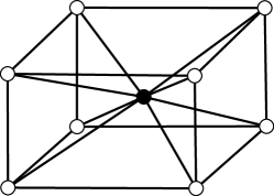
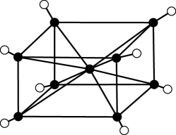
(a)	(b)

Fig. 2: Examples of non-planar graphs where the conductivity is recoverable. The boundary nodes are in white and the interior nodes in black.

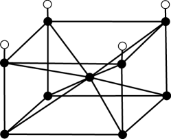
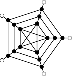
(a)	(b)

Fig. 3: Examples of non-planar graphs where the Schrödinger potential is recoverable. The boundary nodes are in white and the interior nodes in black.

7.3 Examples of indistinguishable conductivities and Schrödinger potentials

We can also get a glimpse of the conductivities (or Schrödinger potentials) that could have the same DtN maps. For the conductivity problem we fix the topology of the graph, choose two directions $\delta\gamma_{1}$ and $\delta\gamma_{2}$, and compute the smallest singular value (rescaled by the largest) of the products of gradients matrix $F(\gamma_{1}(x),\gamma_{2}(y))$, with $\gamma_{1}(x)=1+x\delta\gamma_{1}$ and $\gamma_{2}(y)=1+y\delta\gamma_{2}$, for many $(x,y)\in\mathbb{R}_{0}^{2}$ (the products of gradients matrix is defined in (28)). An example of this is shown if figure 4. Knowing $\sigma_{\min}/\sigma_{\max}$ (the reciprocal of the conditioning number) for $F(\gamma_{1},\gamma_{2})$ is useful when measurements are tainted by noise. Indeed if the norm of the noise relative to norm of the measurements is larger than $\sigma_{\min}/\sigma_{\max}$, then for all practical purposes we may not be able to distinguish these two conductivities $\gamma_{1}$ and $\gamma_{2}$. Thus when there is noise in the data, we may get a set of conductivities that is not of measure zero, but that are indistinguishable from boundary data. This is related to the concept of indistinguishable perturbations in the continuum conductivity problem [25].

We proceed similarly for the Schrödinger problem. We fix $\gamma=1$, choose two Schrödinger potentials $q_{1}$ and $q_{2}$ and compute the smallest singular value (rescaled by the largest) of the product of solutions matrix $G(xq_{1},yq_{2})$ (to be defined in (40)), for many $(x,y)\in\mathbb{R}_{0}^{2}$. This is illustrated in figure 5. The same observation as for the conductivity applies: if the ratio of the norm of the noise to the norm of the measurements is less than $\sigma_{\min}/\sigma_{\max}$ for $G(q_{1},q_{2})$, then for all practical purposes we may not be able to distinguish between $q_{1}$ and $q_{2}$ from boundary measurements.

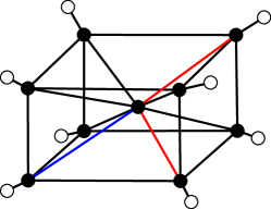
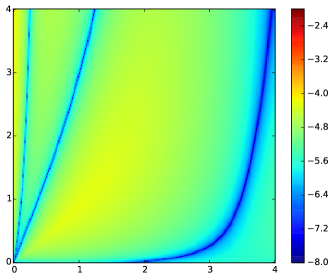
Fig. 4: The smallest singular value (rescaled by the largest) of the product of solutions matrices $F(1+x\delta\gamma_{1},1+y\delta\gamma_{2})$ for the graph in figure 2(b) and $(x,y)\in[0,4]^{2}$. The direction $\delta\gamma_{1}$ (resp. $\delta\gamma_{2}$) is the characteristic function of the red (resp. blue) edges. The color scale on the right corresponds to $\log_{10}(\sigma_{\min}/\sigma_{\max})$.

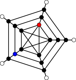
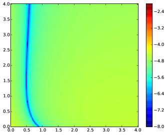
Fig. 5: The smallest singular value (rescaled by the largest ) of the product of solutions matrices $G(xq_{1},yq_{2})$ for the graph in figure 3(b) and $(x,y)\in[0,4]^{2}$. The Schrödinger potential $q_{1}$ (resp. $q_{2}$) is the characteristic function of the red (resp. blue) node. The color scale on the right corresponds to $\log_{10}(\sigma_{\min}/\sigma_{\max})$.

7.4 Statistical study of recoverability

A natural question to ask is how likely is it for a graph to be recoverable? To answer this question we performed the following statistical studies.

7.4.1 Conductivity problem

We used one of the Erdős-Rényi random graph models [23] to generate graphs that have a fixed number of edges $|E|$ and vertices. In this model $|E|$ edges are drawn (uniformly) from all possible $n(n-1)/2$ edges on a graph with $n$ vertices. We choose this particular random graph model because we would like to compare problems with the same number of degrees of freedom. Concretely, the statistical study involved varying two parameters (while keeping $|E|$ fixed): the first is the number of internal nodes $|I|$ and the second the number of boundary nodes $|B|$. To ensure the Dirichlet problem is well posed we draw only graphs that are connected and whose restriction to the interior nodes is connected as well. For each combination of $|I|$ and $|B|$, we draw up to $200$ random graphs connected as a whole and restricted to $I$. In each draw we make up to $20$ trials to make sure the Dirchlet problem is well-posed. The image shown in figure 6(a) represents the (empirical) probability of recoverability for a connected graph (as a whole and restricted to the interior nodes) with $|E|=21$, and $|B|$, $|I|$ given.

There is one phase transition as we vary $|B|$ that can be explained by a counting argument. Indeed the DtN map $\Lambda_{\gamma,0}$ is a symmetric matrix with zero row sums, and is thus determined by $|B|(|B|-1)/2$ scalars. So if $|B|(|B|-1)/2<|E|$ we do not have enough data to recover all edges in the graph. We also see that if there are no interior nodes, then the problem can be solved almost always. However as we increase the number of internal nodes, the graphs on which the conductivity problem is recoverable become scarce. This may be because the random graph model we chose is not adapted to study this particular recoverability problem. We point out that the critical circular planar graphs [19] have much more internal nodes, so recoverability for conductivities seems to be a very rare property (for $|B|=7$, a critical planar graph called “pyramidal network” [19] has $8$ interior nodes).

7.4.2 Schrödinger problem

Here we use the other Erdős-Rényi random graph model [23] to generate graphs with a fixed number of vertices, but where the probability of having an edge between two vertices is $p$. The statistical study consisted of keeping $|I|$ fixed (i.e. the number of degrees of freedom in the Schrödinger potential $q$) and changing two parameters: one is the probability $p$ of having an edge between any two nodes and the other the number of boundary nodes $|B|$. The results are displayed in figure 6(b). As for the conductivity problem we display (out of a maximum $200$ trials) the (empirical) probability of recoverability for a connected graph (as a whole and restricted to the interior nodes) with $|I|=21$ and $|B|$, $p$ given.

We observe two phase transition like properties. The first one follows from a counting argument: if there is not enough data to recover the unknowns then the problem is not recoverable. To be more precise, the DtN map $\Lambda_{\gamma,q}$ is a symmetric $|B|\times|B|$ matrix that is determined by $|B|(|B|+1)/2$ scalars. So if $|B|(|B|+1)/2<|I|$, then the problem is not recoverable. The second is that for probabilities in what appears to be a symmetric interval about $1/2$, the Schrödinger problem is almost always recoverable, whereas elsewhere it is almost always not recoverable. We only have a heuristic explanation for this: if the graph has too little edges, it may not be possible to access certain internal nodes reliably. Also if the graph has too many edges (say it is the complete graph), then it becomes impossible to distinguish the current that flows through the leak from the currents between an internal node an its neighbors. Finally, the interval of edge probabilities for which the Schrödinger problem is recoverable becomes larger as we increase $|B|$. This confirms the intuition that the larger $|B|$ is, the more data we have and the more likely it is for us to find a recoverable graph.

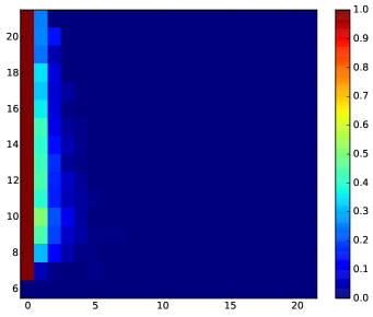
$|B|$	$|B|$
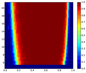
$|I|$	$p$
(a) Conductivity with $|E|=21$	(b) Schrödinger with $|I|=21$

Fig. 6: Statistical study of recoverability.

8 Discussion and future work

Our results generalize existing solvability results for the conductivity and Schrödinger problems on graphs [20, 18, 15, 19, 14, 13, 32, 3, 5, 4] by relaxing what is meant by solvability and allowing conductivities (or Schrödinger potentials) in zero measure sets to have the same boundary data. Thus the problem is ill-posed. If errors are present in the measurements, the ill-posedness is worse since these zero measure sets “expand” to positive measure sets. This is to be expected as even when the discrete conductivity problem is known to be solvable (e.g. the circular planar graph case) the problem become increasingly ill-posed with the size of the network. Studying regularization techniques to deal with this ill-posedness is left for future work.

The complex geometric approach [36, 10] has been successfully used to prove uniqueness for various continuum inverse problems [37]. We believe that the approach presented here can also be extended to other discrete inverse problems, such as the inverse problem of finding the spring constants, masses and dampers in a network of springs, masses and dampers from displacement and force measurements at a few nodes that are accessible.

Finally we would like to use the theoretical results presented here to generalize the numerical methods in [8] to deal with the electrical impedance tomography problem and other related inverse problems in setups that are not necessarily 2D and that involve complex valued quantities. The observation in the numerics (§7) that graphs on which the Schrödinger problem is solvable are much more common than graphs on which the conductivity problem is solvable indicates that to generalize the methods in [8] it may be beneficial to first transform the inverse problem at hand to Schrödinger form (via e.g. the Liouville identity [36]), image a Schrödinger potential and then go back to the original quantity of interest (e.g. the conductivity).

Appendix A Proof of uniqueness a.e. for Schrödinger potentials

We now proceed with the proof of the uniqueness a.e. result (theorem 17). The proof is essentially the same as that for the conductivity case in §5.5, and is included here for completeness. We start by noticing that the product of solutions subspace is spanned by a finite number of vectors. This is the objective of the following lemma, which is stated without proof because of its similarity to lemma 12.

Lemma 24.

Assume the $\gamma,q_{1}$ and $\gamma,q_{2}$ Dirichlet problems are well-posed. Let $u^{(i)}$ (resp. $v^{(i)}$) be $\gamma,q_{1}$ (resp. $\gamma,q_{2}$) harmonic with boundary data $u^{(i)}_{B}=v^{(i)}_{B}=e_{i}$, where $\{e_{i}\}_{i\in B}$ is the canonical basis of $\mathbb{C}^{B}$. Then the product of solutions subspace $Q(q_{1},q_{2})$ is

$$Q(q_{1},q_{2})=\operatorname{span}\left\{{u_{I}^{(i)}\odot v_{I}^{(j)}}\right\}_{i,j\in B}.$$ (38)

The product of solutions space (38) can be rewritten as the range of a matrix,

$$Q(q_{1},q_{2})=\operatorname{\mathcal{R}}(G(q_{1},q_{2})),$$ (39)

where the matrix $G(q_{1},q_{2})\in\mathbb{C}^{|I|\times|B|^{2}}$ is the matrix with columns being all the possible Hadamard products of the columns of $(L_{II}+\mathop{\operator@font diag}\nolimits(q_{1}))^{-1}L_{IB}$ and $(L_{II}+\mathop{\operator@font diag}\nolimits(q_{2}))^{-1}L_{IB}$, i.e.

$$[G(q_{1},q_{2})]_{:,i+(j-1)|B|}=\left[{(L_{II}+\mathop{\operator@font diag}\nolimits(q_{1}))^{-1}L_{IB}}\right]_{:,i}\odot\left[{(L_{II}+\mathop{\operator@font diag}\nolimits(q_{2}))^{-1}L_{IB}}\right]_{:,j},$$ (40)

and the subscript $\gamma$ in the weighted graph Laplacian $L_{\gamma}$ has been omitted for clarity. As in the conductivity case, we want to characterize whether the products of solutions span $\mathbb{C}^{I}$ or not. One way to do this is to look at the determinants

$$g_{\alpha}(q_{1},q_{2})=\det[G(q_{1},q_{2})]_{:,\alpha}$$ (41)

where the matrix $[G(q_{1},q_{2})]_{:,\alpha}$ is the $|I|\times|I|$ submatrix of $G(q_{1},q_{2})$ obtained by selecting the $|I|$ columns corresponding to the multi-index $\alpha\in\{1,\ldots,|B|^{2}\}^{|I|}$. Clearly $Q(q_{1},q_{2})=\mathbb{C}^{I}$ if and only if there is an $\alpha\in\{1,\ldots,|B|^{2}\}^{|I|}$ for which $g_{\alpha}(q_{1},q_{2})\neq 0$. If $|B|^{2}<|I|$, then we always have repeated columns and the determinants are zero. When $|B|^{2}\geq|I|$, the determinant properties guarantee that it is enough to check the $\binom{|B|^{2}}{|I|}$ choices of columns $\alpha=(\alpha_{1},\ldots,\alpha_{|I|})$, with $1\leq\alpha_{1}<\ldots<\alpha_{|I|}\leq|B|^{2}$. This observation is summarized in the following lemma.

Lemma 25.

Assume the Dirichlet problems for $\gamma,q_{1}$ and $\gamma,q_{2}$ are well-posed. The following statements are equivalent

• $Q(q_{1},q_{2})=\mathbb{C}^{I}$

• $\mathop{\operator@font rank}\nolimits G(q_{1},q_{2})=|I|$

• $g_{\alpha}(q_{1},q_{2})\neq 0$ for some $\alpha\in\{1,\ldots,|B|^{2}\}^{|I|}$ with $1\leq\alpha_{1}<\ldots<\alpha_{|I|}\leq|B|^{2}$.

Hence we have the following.

Lemma 26.

Let $\gamma\in\mathbb{C}_{0}^{E}$ and $\zeta$ be such that the Dirichlet problem for $\gamma,q$ is well-posed for all $q\in\mathbb{C}_{\zeta}^{I}$. The functions $g_{\alpha}:\mathbb{C}^{I}_{\zeta}\times\mathbb{C}^{I}_{\zeta}\to\mathbb{C}$ are analytic for any $\alpha\in\{0,\ldots,|B|^{2}\}^{|I|}$.

Proof.

Let $q_{1},q_{2}\in\mathbb{C}^{I}$. First note that the entries of the matrices $((L_{\gamma})_{II}+\mathop{\operator@font diag}\nolimits(q_{k}))^{-1}$, $k=1,2$, are complex analytic on $q_{1}$ and $q_{2}$ when $q_{1},q_{2}\in\mathbb{C}^{I}_{\zeta}$. This is because the cofactor formula for the inverse guarantees that the entries of the matrices in question are rational functions in $q_{1},q_{2}$ which are analytic provided $\det((L_{\gamma})_{II}+\mathop{\operator@font diag}\nolimits(q_{k}))\neq 0$, $k=1,2$. As in the proof of theorem 1, the condition $q_{1},q_{2}\in\mathbb{C}^{I}_{\zeta}$ ensures that $\det((L_{\gamma})_{II}+\mathop{\operator@font diag}\nolimits(q_{k}))\neq 0$, $k=1,2$. Since $G(q_{1},q_{2})$ is obtained from $((L_{\gamma})_{II}+\mathop{\operator@font diag}\nolimits(q_{k}))^{-1}(L_{\gamma})_{IB}$, $k=1,2$ by taking columnwise Hadamard products, each entry of $G(q_{1},q_{2})$ is also analytic on $q_{1}$ and $q_{2}$ when $q_{1},q_{2}\in\mathbb{C}^{I}_{\zeta}$. Finally taking the determinant of a matrix with analytic entries is also analytic. ∎

We can now proceed with the proof of the main result in this section.

Proof of Theorem 17.

By lemma 25, the theorem hypothesis means that there is some multi-index $\beta\in\{1,\ldots,|B|^{2}\}^{|I|}$ such that

$$g_{\beta}(p_{1},p_{2})\neq 0,~{}\text{for some $p_{1},p_{2}\in\mathbb{C}^{|I|}_{\zeta}$}.$$

Thus $g_{\beta}$ is not identically zero. In fact its zero set restricted to $\mathbb{C}^{|I|}_{\zeta}\times\mathbb{C}^{|I|}_{\zeta}$

$$Z(g_{\beta})=\left\{{(q_{1},q_{2})\in\mathbb{C}^{|I|}_{\zeta}\times\mathbb{C}^{|I|}_{\zeta}~{}|~{}g_{\beta}(q_{1},q_{2})=0}\right\},$$ (42)

must be a set of measure zero (see e.g. [28]), where we use the Lebesgue measure on $\mathbb{C}^{|I|}\times\mathbb{C}^{|I|}$. By lemma 25, the subset $S$ of $\mathbb{C}^{I}_{\zeta}\times\mathbb{C}^{I}_{\zeta}$ on which $Q(q_{1},q_{2})\neq\mathbb{C}^{I}$ is

$$S=\bigcap_{\alpha\in\{1,\ldots,|B|^{2}\}^{|I|}}Z(g_{\alpha}).$$

Since $Z(g_{\beta})$ has measure zero, the set $S\subset Z(g_{\beta})$ must have measure zero as well by monotonicity of the Lebesgue measure. ∎

References

- [1] G. Alessandrini, Remark on a paper by H. Bellout and A. Friedman: “Identification problems in potential theory” [Arch. Rational Mech. Anal. 101 (1988), no. 2, 143–160; MR0921936 (89c:31003)], Boll. Un. Mat. Ital. A (7), 3 (1989), pp. 243–249.
- [2] K. Ando, Inverse scattering theory for discrete Schrödinger operators on the hexagonal lattice, Annales Henri Poincaré, 14 (2013), pp. 347–383. doi:10.1007/s00023-012-0183-y.
- [3] C. Araúz, A. Carmona, and A. Encinas, Dirichlet-to-Robin matrix on networks, Electronic Notes in Discrete Mathematics, 46 (2014), pp. 65 – 72. Jornadas de Matemática Discreta y Algorítmica. doi:10.1016/j.endm.2014.08.010.
- [4] , Dirichlet-to-Robin maps on finite networks, Applicable Analysis and Discrete Mathematics, 9 (2015), pp. 85–102. doi:10.2298/AADM150207004A.
- [5] , Overdetermined partial boundary value problems on finite networks, Journal of Mathematical Analysis and Applications, 423 (2015), pp. 191–207. doi:10.1016/j.jmaa.2014.09.025.
- [6] S. R. Arridge, Optical tomography in medical imaging, Inverse Problems, 15 (1999), pp. R41–R93. doi:10.1088/0266-5611/15/2/022.
- [7] L. Borcea, Electrical impedance tomography, Inverse Problems, 18 (2002), pp. R99–R136. Topical Review. doi:10.1088/0266-5611/18/6/201.
- [8] L. Borcea, V. Druskin, F. Guevara Vasquez, and A. V. Mamonov, Resistor network approaches to electrical impedance tomography, in Inside Out II, G. Uhlmann, ed., vol. 60, MSRI Publications, 2012.
- [9] L. Borcea, F. Guevara Vasquez, and A. V. Mamonov, Numerical solution of the 2D inverse absorptive Schrödinger problem with a discrete Liouville identity. in preparation.
- [10] A.-P. Calderón, On an inverse boundary value problem, in Seminar on Numerical Analysis and its Applications to Continuum Physics (Rio de Janeiro, 1980), Soc. Brasil. Mat., Rio de Janeiro, 1980, pp. 65–73.
- [11] M. Cheney, D. Isaacson, and J. C. Newell, Electrical impedance tomography, SIAM Rev., 41 (1999), pp. 85–101 (electronic). doi:10.1137/S0036144598333613.
- [12] F. R. K. Chung, Spectral graph theory, vol. 92 of CBMS Regional Conference Series in Mathematics, Published for the Conference Board of the Mathematical Sciences, Washington, DC, 1997.
- [13] S.-Y. Chung, Identification of resistors in electrical networks, J. Korean Math. Soc., 47 (2010), pp. 1223–1238. doi:10.4134/JKMS.2010.47.6.1223.
- [14] S.-Y. Chung and C. A. Berenstein, -harmonic functions and inverse conductivity problems on networks, SIAM J. Appl. Math., 65 (2005), pp. 1200–1226 (electronic). doi:10.1137/S0036139903432743.
- [15] Y. Colin de Verdière, Réseaux électriques planaires. I, Comment. Math. Helv., 69 (1994), pp. 351–374. doi:10.1007/BF01585564.
- [16] , Spectres de graphes, vol. 4 of Cours Spécialisés [Specialized Courses], Société Mathématique de France, Paris, 1998.
- [17] Y. Colin de Verdière, I. Gitler, and D. Vertigan, Réseaux électriques planaires. II, Comment. Math. Helv., 71 (1996), pp. 144–167. doi:10.1007/BF02566413.
- [18] E. Curtis, E. Mooers, and J. Morrow, Finding the conductors in circular networks from boundary measurements, RAIRO Modél. Math. Anal. Numér., 28 (1994), pp. 781–814.
- [19] E. B. Curtis, D. Ingerman, and J. A. Morrow, Circular planar graphs and resistor networks, Linear Algebra Appl., 283 (1998), pp. 115–150. doi:10.1016/S0024-3795(98)10087-3.
- [20] E. B. Curtis and J. A. Morrow, Determining the resistors in a network, SIAM J. Appl. Math., 50 (1990), pp. 918–930. doi:10.1137/0150055.
- [21] E. B. Curtis and J. A. Morrow, Inverse Problems for Electrical Networks, vol. 13 of Series on Applied Mathematics, World Scientific, 2000.
- [22] K. A. Dines and R. J. Lytle, Analysis of electrical conductivity imaging, Geophysics, 46 (1981), pp. 1025–1036. doi:10.1190/1.1441240.
- [23] P. Erdős and A. Rényi, On random graphs. I, Publ. Math. Debrecen, 6 (1959), pp. 290–297.
- [24] S. Ervedoza and F. de Gournay, Uniform stability estimates for the discrete Calderón problems, Inverse Problems, 27 (2011), p. 125012. doi:10.1088/0266-5611/27/12/125012.
- [25] D. G. Gisser, D. Isaacson, and J. C. Newell, Electric current computed tomography and eigenvalues, SIAM J. Appl. Math., 50 (1990), pp. 1623–1634. doi:10.1137/0150096.
- [26] G. H. Golub and C. F. Van Loan, Matrix computations, Johns Hopkins Studies in the Mathematical Sciences, Johns Hopkins University Press, Baltimore, MD, fourth ed., 2013.
- [27] F. Guevara Vasquez. Julia code accompanying this paper is available online. Available from: http://www.math.utah.edu/~fguevara/recov.
- [28] R. C. Gunning and H. Rossi, Analytic functions of several complex variables, Prentice-Hall, Inc., Englewood Cliffs, N.J., 1965.
- [29] R. A. Horn and C. R. Johnson, Matrix analysis, Cambridge University Press, Cambridge, second ed., 2013.
- [30] V. Isakov, Inverse problems for partial differential equations, vol. 127 of Applied Mathematical Sciences, Springer, New York, second ed., 2006.
- [31] H. Isozaki and E. Korotyaev, Inverse problems, trace formulae for discrete Schrödinger operators, Ann. Henri Poincaré, 13 (2012), pp. 751–788. doi:10.1007/s00023-011-0141-0.
- [32] T. Lam and P. Pylyavskyy, Inverse problem in cylindrical electrical networks, SIAM J. Appl. Math., 72 (2012), pp. 767–788. doi:10.1137/110846476.
- [33] H. Morioka, Inverse boundary value problems for discrete Schrödinger operators on the multi-dimensional square lattice, Inverse Probl. Imaging, 5 (2011), pp. 715–730. doi:10.3934/ipi.2011.5.715.
- [34] J. Nocedal and S. J. Wright, Numerical optimization, Springer Series in Operations Research and Financial Engineering, Springer, New York, second ed., 2006.
- [35] M. Salo, Calderón problem, 2008. Lecture notes. Available from: http://www.rni.helsinki.fi/~msa/teaching/calderon/calderon_lectures.pdf.
- [36] J. Sylvester and G. Uhlmann, A global uniqueness theorem for an inverse boundary value problem, Ann. of Math. (2), 125 (1987), pp. 153–169. doi:10.2307/1971291.
- [37] G. Uhlmann, Developments in inverse problems since Calderón’s foundational paper, in Harmonic analysis and partial differential equations (Chicago, IL, 1996), Chicago Lectures in Math., Univ. Chicago Press, Chicago, IL, 1999, pp. 295–345.
- [38] G. Uhlmann, Electrical impedance tomography and Calderón’s problem, Inverse Problems, 25 (2009), p. 123011. doi:10.1088/0266-5611/25/12/123011.