A survey of discrete methods in (algebraic) statistics for networks

Abstract.

Sampling algorithms, hypergraph degree sequences, and polytopes play a crucial role in statistical analysis of network data. This article offers a brief overview of open problems in this area of discrete mathematics from the point of view of a particular family of statistical models for networks called exponential random graph models. The problems and underlying constructions are also related to well-known concepts in commutative algebra and graph-theoretic concepts in computer science. We outline a few lines of recent work that highlight the natural connection between these fields and unify them into some open problems. While these problems are often relevant in discrete mathematics in their own right, the emphasis here is on statistical relevance with the hope that these lines of research do not remain disjoint. Suggested specific open problems and general research questions should advance algebraic statistics theory as well as applied statistical tools for rigorous statistical analysis of networks.

1. Introduction

The development of a rich literature on networks in the past decade has left ample opportunities for complementary mathematically rigorous results that should serve as the foundation for statistical modeling and fast computation of network features. In this review, we focus on exponential families for random graphs, models over equivalence classes of graphs summarized by a selected set of graph or network summary statistics. Here, the word ‘model’ is used in the statistical sense, and the terms ‘graph’ and ‘network’ are used interchangeably. Introductory paragraphs of Sections 3 and 4 offer an answer to the following question: Why consider statistics when studying random graphs and networks? A summarized answer can be phrased as follows: how a network is generated is crucial to properly calculate statistical network properties and specify the distributions being sampled. This includes properties that depend on both degrees of nodes in the network, higher-order degree correlations, or other, possibly global, summary statistics; cf.  an excellent example and the concluding paragraph in [Jac08, Section 4.2.1].

The reader may wonder why the focus on exponential families for random graphs, or ERGMs. While being able to write a random graph model as an exponential family is not impressive in and of itself, understanding the geometry, algebra, and the discrete structures supporting the model offer various statistical insights that are the theme of this chapter. A recent computer science article [BDE] shows that ERGMs are ‘hard’, that is, their normalizing constants are incomputable in general. While this important result about inapproximability in polynomial time formalizes the inherent complexity of this family of models, as a statistical model family they are still very broad and rich and have desirable properties. As such, they in the very least offer the theoretical foundation for studying random graphs and networks, and a bedrock for algorithmic exploratory analysis of sampling distributions of various graph summary statistics.

The statistics literature on understanding and developing network models is ever-growing; a partial list of references is offered below in context. Within this realm, though, the basic problem of establishing rigorous procedures for statistical inference is still a challenge, due to the varying complexity of the models and types of properties of data they capture, as well as networks being a novel data type in terms of traditional statistics.

The motivating problem for this discussion is thus a basic one of statistical inference, tightly related to several fundamental tasks required for statistical analysis of (any kind of) data: parameter estimation, sampling from the distributions in the model, testing model/data fit, and model selection. The broad goal of statistical inference is to decide, with a high degree of confidence, whether an observed data sample $x=x_{1},\dots,x_{N}$ can be regarded as a draw from a distribution $p_{\theta_{0}}\in\mathcal{M}$ coming from a candidate statistical model $\mathcal{M}$, specified by the unknown parameter $\theta_{0}$. Of course, this entails two crucial steps: 1) estimation: use the observed data $x$ to produce an optimal estimate $\hat{\theta}=\hat{\theta}(x)$ of $\theta_{0}$; and 2) goodness-of-fit testing: assess whether $p_{\hat{\theta}}$ can be considered a satisfactory generative model for the observed data $x$. Surprisingly, these fundamental tasks pose a family of open problems, in particular for discrete sparse small-sample data such as networks [KK15, HGH08, HL81, Hab81, Agr92, YLZ, CKHG15, CDS11]. These problems and their natural connection to discrete structures are the focus of this short overview.

In the remainder of the chapter, we will use the $\beta$ model for random graph, defined in Example 2.1, as a running example to illustrate the structure and implications of various statistical modeling questions that discrete mathematics tools can answer.

2. Preliminaries

We begin with some technical preliminaries on linear ERGMs and statistical considerations about these models. A statistical model $\mathcal{M}$ is a family of probability distributions indexed by a set of parameters $\Theta\subset\mathbb{R}^{n}$. In exponential random graph models, or ERGMs for short, one first selects the network characteristic $T$ of interest in a particular problem. This selection is done so that $T$ represents some interpretable and meaningful summary statistic of a network. The resulting model is then the collection of probability measures

$$\mathcal{M}=\{p_{\theta}:\theta\in\Theta\},$$

indexed by points in $\Theta\subseteq\mathbb{R}^{n}$ such that, for any $\theta\in\Theta$, the probability of observing a given network $G=g$ takes on the exponential form

(2.1) $$p_{\theta}(g)=\exp\{\langle T(g),\theta\rangle-\psi(\theta)\},$$

where $\psi(\theta):=\sum_{g}\exp\{\langle T(g),\theta\rangle\}$ is a normalizing function called the log-partition function, and $T(g)$ is the vector of minimal sufficient statistics for the model. The exponential form of the probabilities above is a central theme in statistical theory, and statistical models of this form, known as exponential families, are known to exhibit optimal statistical performance and appear with a growing appeal in the machine learning community as well. Consistent with the running examples, we are considering linear exponential families for now, that is, $\langle T(g),\theta\rangle$ is a linear map of the state space. General exponential families can use non-linear maps, of course. For a more detailed statistical treatment of this family of models the reader is referred to classical references [Bro86], [BN14] and [LC83, LC98], as well as a more recent book [BD15]. ERGMs are, effectively, models over equivalence classes of networks, where two networks $g_{1}$ and $g_{2}$ are regarded as probabilistically equivalent whenever $T(g_{1})=T(g_{2})$. Conditioning on the values of $T$ permits the reduction of the data through sufficient statistics and thus eliminates nuisance parameters [Agr92], which can be very helpful in applications.

Example 2.1 (The $\beta$ model for graphs).

The $\beta$ model for graphs is a well-known statistical model for random undirected graphs. In its original form, the $\beta$ model considers simple graphs, that is, does not allow loops or multiple edges; but the general version allows edges to appear with bounded multiplicity. It essentially assigns parameters $\beta_{1},\dots,\beta_{n}$ to the $n$ vertices in the network that measure their ‘friendliness’, or propensity to attract edges. The edges are then assumed to be independent and appear with probability proportional to the product of the parameters of its vertices; in symbols:

$$Prob(G=g)\propto\prod_{\{i,j\}\in E(g)}\beta_{i}\beta_{j}=\prod_{i=1}^{n}\beta_{i}^{\deg(i)},$$

where ‘$\propto$’ refers to the fact that the resulting quantity should be normalized by the log-partition function. In this model, the sufficient statistics vector $T(g)$ is the degree sequence of the graph $g$. Indeed, the model is usually given directly in the exponential family form (2.1) with $T(g)=(d_{1},\dots,d_{n})$ being the degree sequence of $g$:

(2.2) $$p_{\beta}(g)=\exp\{\sum_{i=1}^{n}d_{i}\beta_{i}-\psi(\beta)\}.$$

For a brief history of the model, see for example the introduction and references given in [RPF13], which deals with the general version of the $\beta$ model and the special case of the simple graph version studied in [CDS11].

The $\beta$ model (2.2) is indeed one of the simplest interpretable undirected random graph models of relevance in statistical applications. In fact, the study of the degree sequences and, in particular, of the degree distributions of real networks is a classical topic in network analysis, which has received extensive treatment in the statistics literature (starting with, e.g., [HL81], [FW81], [FMW85]), the physics literature (e.g. [NSW01], [New03], [PN04], [WAD09]) as well as in the social network literature (e.g., [RPKL07], [Goo07], [HM07], and references therein). See also the monograph by [GZFA09] and the books by [Kol09] and [New10]. Its known properties can be used as a blueprint for consideration of more complex models. Specifically, it is a very nice and well-understood ERGM from the following points of view that simultaneously serve as an outline of the remainder of this chapter:

1. Exact inference for model fitting: exact testing is used for testing goodness of fit of a model when applicability of standard statistical asymptotic methods is unclear. Typically, this is the case for small sample sizes $N$, and also largely remains a problem for network data in particular. These topics are the content of Section 3.

   1. For the $\beta$ model, exact testing depends on sampling graphs with a prescribed degree sequence, for which there are several algorithms throughout the statistics, computer science and graph theory literatures. The general problem is wide open for other ERGMs.

   2. To construct an appropriate Markov chain for exact testing, sampling graphs with fixed properties should be done within the context of a statistical model.

   3. As we will see, all linear ERGMs reduce to hypergraph degree sequence problems.

2. Parameter estimation and noisy data: Viewing random graph models through the lens of exponential families offers a way to capture the issue of existence of maximum likelihood estimators (MLE), a fundamental problem that is largely unexplored. The problem and its statistical implications are explained in Section 4.

   1. For the $\beta$ model, the geometry of MLE existence is captured by the convex hull of all degree sequences. The extreme points of that polytope correspond to threshold graphs and facet-defining inequalities have been characterized. In general, the geometry of MLE existence is captured by the model polytope, whose lattice points are realizable sufficient statistics vectors. These polytopes are not known for other ERGMs.

   2. In data privacy considerations, or in dealing with noisy data, observed sufficient statistics may contain errors and thus in particular may not be realizable by any graph. For the $\beta$ model, it is known when an integer sequence is graphical, i.e., when there exists a graph that realizes the sequence as its degree sequence. The general problem of characterizing realizable sufficient statistic vectors is wide open yet crucial for establishing reliability of inference.

   3. Efficient facet description of the model polytope for other examples of ERGMs would be crucial to develop appropriate tools for dealing with noise in the data.

3. The model has desirable asymptotic properties [CDS11], closely related to graphons [LS06]. As the asymptotics are different than the asymptotics mentioned in item (1) above, we will not discuss these issues in this Chapter, but instead point the interested reader to [WO] and for a quick list of references to [RPF13, Introduction].

Here are examples of some other models that build on the $\beta$ graph model and for which many of these questions remain open. In the interest of space and readability, equations repeating the structure (2.1) for each case are omitted but can easily be found in the references.

Example 2.2.

The joint degree matrix model is the ERGM of the form (2.1) where the sufficient statistic $T(g)$ is the joint degree matrix, or JDM for short, of $g$. The JDM counts the number of edges between nodes of given degrees, for all degree pairs. The model, as an ERGM, was introduced to the statistics literature in recent work [SR14b], motivated by previous lines of research outside of mainstream statistics, such as [EMT15], which offers a fast mixing algorithm and a fantastic introduction and overview of the joint degree matrix as a network statistic, and [SP12].

As pointed out in [EMT15], fixing the value of the JDM of a network is stronger than just fixing the degree sequence, though it uniquely defines the degree sequence.

Example 2.3.

The $\beta$ model for hypergraphs was introduced in [SSR⁺14]. It looks identical to the $\beta$ model for graphs, except the edges in the network $g$ can be of size larger than $2$. In particular, there are three variants: uniform, layered uniform, and general. In the uniform variant, hyperedges of fixed size $k$ occur independently with probability proportional to $\beta_{i_{1}}\cdots\beta_{i_{k}}$ for all $k$-tuples $i_{1},\dots,i_{k}$ of vertices on the graph. The sufficient statistic in the this case is the hypergraph $k$-degree sequence, that is, the number of edges of size $k$ to which each vertex belongs.

In the layered variant, the set of possible hyperedges is extended to include edges of all sizes up to and including some fixed size $k$. The sufficient statistics are thus layered hypergraph degree sequences: the number of hyperedges of each size, $2,\dots,k$, to which a vertex belongs. In the general variant, all edge sizes are allowed, and the model is more complicated; for details see [SSR⁺14].

Example 2.4.

The $p_{1}$ model for random graphs assigns probabilities to directed edges in a random graph according to the propensity of the nodes to receive, send, or reciprocate edges. The sufficient statistics vector $T(g)$ of the model consists of: the in-degrees of all nodes, out-degrees of all nodes, and the number of reciprocated edges, where a reciprocated edge is of the form $i\leftrightarrow j$. The model has a history in statistic and applications, see for example [HL81], [FW81] and [PRF10]. The last reference interprets the model through the lens of algebraic statistics and studies its linear ERGM structure in terms of algebra and geometry; cf. [RPF13].

A fairly recent extended review article on statistical network models [GZFA09] offers many other examples of models, beyond linear ERGMs, whose geometric and combinatorial properties are yet to be explored.

3. Sampling algorithms in exact testing

Testing the fit of the model means deciding whether the model provides a plausible probabilistic representation of the available data. Unfortunately, most tests for goodness of fit are based on large sample approximations that are not applicable to data such as sparse contingency tables used in, for example, cross-classification of categorical variables, or data such as random graphs that can be naturally thought of as contingency tables through incidence matrices. Fundamental examples of inadequacy of the use of asymptotic approximations were already pointed out over two decades ago in statistics literature [Hab88], [Agr92]: when sample size $N$ is small, or for example if some data table cell entries are much smaller than others, exact testing should be performed instead. Even so, a large part of the literature on, say, network computation and modeling does not address the lack of model fitting and testing methodology beyond heuristic algorithms [Han03, CKHG15, HGH08]. This is largely due to the inherent model complexity or degeneracy and the lack of tools that can handle network models and sparse small-sample data.

The role and relevance of discrete mathematics in exact testing is as follows. In an exact test for a model with sufficient statistics vector $T$, the observed data $x$ with $T(x)=t_{obs}$ is compared to a reference set

$$\mathcal{F}_{t_{obs}}:=\{y:T(y)=t_{obs}\}$$

of data with the same value of the sufficient statistic. This reference set is also called the fiber in algebraic statistics literature. It is a fiber of the algebraic map that computes the sufficient statistics; in the $\beta$ model case the map is linear, since node degrees can be computed as row/column sums of the incidence matrix. Note that, by definition of sufficiency, the probability of any data point in the fiber is determined completely by the value $t_{obs}$, hence the fiber is a good reference set to consider for testing. Using a suitable choice of a goodness-of-fit statistic that measures, for example, the distance of the data $x$ from the expected value under the model, the simulated data points in $\mathcal{F}_{t_{obs}}$ are compared to the observed data. If a relatively large number of those are closer to the expected value than the observed data, than one declares poor model fit. These are, roughly, the essential elements of an exact test, whose name refers to the exact conditional distribution of data points in the fiber $\mathcal{F}_{t_{obs}}$, where we are conditioning on the observed value $t_{obs}$ of the sufficient statistics.

To visualize the elements of an exact conditional test, consider the following example. Suppose the observed graph is $g_{1}$ in Figure 2; see [OHT13, Figure 13] and [GPS, Section 4.1]. Given the degree sequence of $g_{1}$, the expected value under the model is visualized as a weighted graph whose edge weights are the expected values of the random variables representing the edges. This is computed using the MLE of the parameters; see Equation (4.1). One may view these expected values as computing the relative frequency of the edges in the set of all graphs whose degree sequence equals that of the graph $g_{1}$. For example, the edge $\{3,4\}$ appears in 15% of graphs that realize this degree sequence, and since the conditional distribution on the fibers of the $\beta$ model is uniform, this frequency doesn’t need to be weighted to compute the expected values. Intuitively, the exact test is meant to assesses the relative closeness of the observed graph to the expected graph, and thus it answers the question: is $g_{1}$ more like the expected graph than the graphs $g_{2},g_{3},g_{4}$ from Figure 2 and the other $587$ graphs in the fiber?

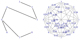
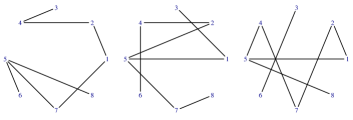
Figure 1. Observed graph $g_{1}$ (left) with degree sequence (2,1,1,2,3,1,2,1), and the expected probability-weighted graph under the $\beta$ model.

Figure 2. Three out of the $590$ other graphs in the fiber $\mathcal{F}_{(2,1,1,2,3,1,2,1)}$: $g_{2}$ (left), $g_{3}$ (center), $g_{4}$.

There are two important points to be made before we discuss the key problem. First, choosing a good goodness-of-fit statistic is in general an open problem, and is difficult in particular in random graph models for which edges are not independent random variables. For a discussion of the special case of 2-way contingency table models, see [Agr92, §3.1]. Second, a good example of a goodness-of-fit statistics to use for random graphs with independent edges is the chi-square statistic, which simply computes the square of the weighted Euclidean distance in $\mathbb{R}^{n}$ between the observed graph and the expected graph (or MLE). It is defined as:

$$\chi^{2}(g):=\sum_{i,j}\frac{(\hat{g}_{ij}-g_{ij})^{2}}{\hat{g}_{ij}},$$

where $g_{ij}$ is $1$ if the edge $\{i,j\}$ is present in $g$ and $0$ otherwise, and $\hat{g}_{ij}\in(0,1)$ is the expected value of the random variable representing the edge $\{i,j\}$ under the MLE, as illustrated in Figure 2. The values of the chi-square statistic for the four graphs above are:

$$\chi^{2}(g_{1})=19.49,\quad\chi^{2}(g_{2})=17.42,\quad\chi^{2}(g_{3})=21.56,\quad\chi^{2}(g_{4})=26.53.$$

To determine whether the value $\chi^{2}(g_{1})$ is too large, one should enumerate the fiber and compute the value of the statistic for all $591$ graphs in it.

As it is computationally prohibitive to enumerate the fiber except in very small cases, one tries to instead sample from the fiber and estimate the number of data points that are more extreme than the observed, with respect to the chosen goodness-of-fit statistic. Thus the key problem in the exact testing procedure is that of exploring the fiber through sampling from the conditional distribution given $t_{obs}$.

Problem 3.1 (General Problem 1).

Fix a random graph model $\mathcal{M}$ with sufficient statistics $T$. Develop an efficient algorithm that samples from the space of graphs with arbitrary fixed value of $T(g)=t_{obs}$.

A fiber sampling algorithm can be a direct sampler or it can be based on a Markov chain and used through the Metropolis algorithm, which is a standard algorithm and can be found, for example, in [RC99]. The algebraic statistics literature focuses on the latter. The reason for this is the natural connection to algebraic geometry. Namely, the theoretical feasibility of constructing Markov chains to solve General Problem 1 for arbitrary linear ERGMs, as well as finiteness of the complexity of steps needed to perform the Markov chain random walk on fibers of every log-linear model, form a cornerstone of traditional algebraic statistics through a fundamental theorem from [DS98]; see also [DSS09, Theorem 1.3.6]. Its applied solution and relevance in exact testing for any linear ERGM hinges upon the development of efficient sampling algorithms for graphs and hypergraphs, as outlined here.

The steps or moves needed to perform the Markov chain above for a a given model are called Markov moves. A Markov basis for a model is a collection of moves guaranteed to connect each fiber of that model. A move is an element of the Graver basis of the model if it contains no proper sub-moves; see Figure 3 for a running example.

Remark 3.2.

In order to be of statistical relevance, and make any inference from the observed data, Problem 3.1 should be solved within the context of a statistical model. In other words, when a network feature, or a set thereof, is fixed in sampling, it is understood that the feature can serve as a sufficient statistic of some model; the statisticians then ask to identify the model and study its various properties in order to determine feasibility and reliability of inference and model fitting.

Example 3.3.

For the $\beta$ model for random graphs from Example 2.1, the reference set $\mathcal{F}_{t_{obs}}$ is the set of graphs whose degree sequence $d$ equals the degree sequence $t_{obs}:=d(g)$ of the observed graph $g$. It is easy to see that in the $\beta$ model the conditional probability distribution of graphs given a fixed observed degree sequence is uniform; in general, of course, this distribution depends on the model. Therefore, in the $\beta$ model, as well as others we discuss in this chapter as the reader may easily verify, graphs should be sampled uniformly, because conditioning on the sufficient statistics results in the uniform distribution on the fiber.

Of course, Problem 3.1 has been solved for the $\beta$ model for graphs. Indeed, various algorithms for constructing random graphs with a fixed degree sequence - in other words, sampling the fibers of the $\beta$ model - have been proposed over the years, with or without the context of the model, and the reader is probably familiar with the graph theory literature on this topic, most relevant part of which is cited throughout this Chapter. On the statistics side, [BD10] derive a sequential importance sampling algorithm for this model. A different random generation algorithm for simple connected graphs can be found in [VL05].

As mentioned above, one could think of solving the sampling problem in different ways: by an algorithm that constructs, uniformly at random, a graph that realizes the given degree sequence (where care should be taken that such an algorithm can, in fact, discover the entire fiber!); or by finding a set of moves, sometimes also called ‘edge swaps’ in graph theory, that can serve as a basis for a Markov chain Monte Carlo (MCMC) sampling algorithm on the fiber. Here the word ‘basis’ is used in a technical sense but can also be understood intuitively: the moves should guarantee to discover the entire fiber and define a symmetric, aperiodic chain on any given fiber of the model. The Markov chain approach offers a nice alternative and an interesting connection to other areas of mathematics. As such, it is largely the focus of the remainder of this section.

3.1. Ingredients for a Markov chain fiber sampler

In order to use the MCMC method to sample the fiber of an observed graph, three important questions should be answered. First, a Markov basis should be specified: a set of moves that the algorithm uses to go from any graph to any other graph in any fiber. Second, the stationary distribution of the proposed Markov chain should be the correct conditional distribution; recall that in the $\beta$ model example, it should be uniform. Third, mixing time considerations cannot be avoided in this approach - one can easily propose seemingly straightforward Markov chains that have extremely unreasonable behavior in that they will take a very long time to converge or to explore the fiber.

One way to answer the first two questions simultaneously is through the use of algebraic statistics. The third question on mixing time is discussed subsequently.

There is an algebraic geometry or, if you will, commutative algebra equivalent to a Markov basis for a linear ERGM stemming from the fundamental theorem from [DS98]. Namely, every such statistical model lies in a natural algebraic variety: A variety is the set of all solutions to a system of polynomial equations, and those encoding parametric statistical models can equivalently be described parametrically – there is an algebra-geometry duality here; see the excellent introductory explanation in [SKKT00, §2.4 and 2.5]. Focusing on the algebra, the parametrization is encoded via a homomorphism between two polynomial rings, say $\phi:\mathbb{C}[E]\rightarrow\mathbb{C}[\theta_{1},\dots,\theta_{n}]$, where $E$ is some set of variables, and $\theta_{i}$ are parameters. The indeterminates in the two polynomial rings carry a special meaning in algebraic statistics: $E$ represent random variables of interest, while $\theta=(\theta_{1},\dots,\theta_{n})$ is the vector of unknown model parameters. For example, in the case of ERGMs whose edges are independent random variables, $E=E(G)$ are edges of the random graph $G$. The kernel of the map $\phi$ is an ideal in the polynomial ring $\mathbb{C}[E]$, and this ideal is the defining ideal of the algebraic variety whose real positive part contains the statistical model. Readers interested in further algebraic details of this correspondence may consult [DSS09, page 25].

Example 3.4.

In the specific case of the $\beta$ model for graphs with no statistical sampling constraints, the graph $G$ is the complete graph because all edges are allowed to appear in the random graph realization $g$. The homomorphism $\phi$ maps each edge $e_{ij}$ to the product of the parameters $\beta_{i}\beta_{j}$. For example, consider the random graph $\beta$ model on $n=8$ nodes. The coordinate map corresponding to the parameterization of the model is

$$\phi_{K_{8}}:\mathbb{C}[e_{12},e_{13},\dots,e_{78}] \rightarrow\mathbb{C}[\beta_{1},\dots,\beta_{8}]$$

$$e_{ij} \mapsto\beta_{i}\beta_{j}.$$

Note that here we have forgotten the exponential and the normalizing constant because they do not affect the algebraic structure of the parametrization, so by abuse of notation we drop the ‘$\exp$’ from the model specification. An example of an equation that vanishes on the model is $e_{17}e_{24}e_{34}e_{58}-e_{14}e_{23}e_{45}e_{78}$. The algebraic relation holds because $\phi_{K_{8}}(e_{17}e_{24}e_{34}e_{58})=\phi_{K_{8}}(e_{14}e_{23}e_{45}e_{78})$ since, of course, the two graphs on edge sets $\{17,24,34,58\}$ and $\{14,23,45,78\}$ have the same degree sequence, which is the sufficient statistic for the model; refer to Figure 3. Note that the equation vanishing on the model is equivalent to saying that equation is in the kernel of the coordinate map: $e_{17}e_{24}e_{34}e_{58}-e_{14}e_{23}e_{45}e_{78}\in\ker\phi_{K_{8}}$.

To summarize: probability distributions in the model correspond to real positive points on an algebraic variety, where the parametric description of the model gives rise to the parametrization of the variety. This variety is defined implicitly by the equations that vanish on the model. Coordinates of the polynomial ring that is the domain of $\phi$ correspond to the joint probabilities of random variables in the model. Equations that vanish on the variety represent algebraic relations among the joint probabilities. To visualize what these relations mean, consider $\prod_{\{i,j\}\in E^{+}}e_{ij}-\prod_{\{i,j\}\in E^{-}}e_{ij}$, for two sets of edges $E^{+}$ and $E^{-}$. This is an equation that vanishes for all points on the model (i.e., a relation on the edges) if and only if the graphs whose edges sets are $E^{+}$ and $E^{-}$ have the same probability under the model. In turn this happens if and only if the two subgraphs have the same values of the sufficient statistics vector. In the linear ERGM case, the variety has a special structure called toric, due to linearity, and as a consequence the defining equations are all binomials.

The crucial observation is then that such binomials correspond to moves on the fibers of the model, and in fact the moves comprise a Markov basis if and only if the binomials suffice to generate all equations that vanish on the variety [DS98]. This fact is sometimes called the fundamental Theorem of Markov Bases. This correspondence should be interpreted in the following way: $h_{1}-h_{2}$ is a defining equation of the variety corresponding to the model if and only if replacing the subgraph $h_{2}\subset g$ by the subgraph $h_{1}\subset g$ is a move on the fiber of the model, meaning that the move does not change the value of the sufficient statistics vector, as illustrated in Figure 3.

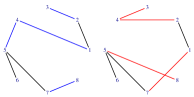
Figure 3. A Markov move under the $\beta$ model for the graph $g=g_{1}$ from Figure 2: the graph $g_{1}$ with edges $h_{2}$ to be removed in blue (left), and the resulting graph $g_{2}$ from Figure 2 after $h_{2}$ is replaced by edges in $h_{1}$ which is shown in red. Note that this move $h_{1}-h_{2}$ is not a minimal one, cf. Figure 4. Instead, it is an example of a Graver move. If structural zeros were present in the model, moves like this one may be needed for connecting the fiber.

In fact, the correspondence applies to general log-linear models for discrete data, not only networks, and is one of the cornerstones of algebraic statistics. In the general case the moves $h_{1}-h_{2}$ need not be squarefree and need not represent graphs; instead each $h_{1}$ and $h_{2}$ can be an arbitrary monomial in the indeterminates $E$ and this machinery works for general contingency table models. Simple graphs are just 0/1 contingency tables, while graphs can in general be represented by non-negative tables, where each positive entry indicates presence of an edge, with multiplicity if the model allows for it. Given the very extensive literature on this topic, for example summarized in the recent book [AHT12] and references given therein, let us not spend more time studying details of this equivalence here. Instead, we pause to note the important consequences: By a fundamental theorem in commutative algebra called the Hilbert basis theorem, a Markov basis exists and is finite for every linear ERGM. Furthermore, using the moves from a Markov basis given by the algebraic correspondence theorem to generate moves in the Metropolis algorithm automatically converges to the correct stationary distribution on the fiber. Note that, by definition, any set of moves containing a minimal Markov basis has the same property.

The $\beta$ model for graphs from Example 3.3 somehow seems to have a parallel history in various literature, as reflected upon in the following Remark.

Remark 3.5.

In commutative algebra, Markov bases for the $\beta$ model exist under the name of generators of toric ideals of graphs. This name comes from the fact that the moves from the $\beta$ model can be encoded by closed alternating walks on graphs: sets of edges partitioned into two sets, $E^{+}$ and $E^{-}$, such that they constitute a closed walk when traversed in alternating order $e_{1},\dots,e_{m}$ with $e_{i}\in E^{+}$ for even $i$ and $e_{i}\in E^{-}$ for odd $i$. For example, the move corresponding to removing blue and adding red edges in Figure 3 represents one such alternating walk, with $E^{+}$ and $E^{-}$ corresponding to red and blue edges, respectively. The reader will note that this move can be obtained as a sequence of three moves represented by closed 4-cycles illustrated in Figure 4. Equivalently, the polynomial $e_{17}e_{24}e_{34}e_{58}-e_{14}e_{23}e_{45}e_{78}$ lies in the ideal generated by the three polynomials representing the 4-cycles: $e_{17}e_{24}e_{34}e_{58}-e_{14}e_{23}e_{45}e_{78}=e_{24}e_{34}(e_{17}e_{58}-e_{15}e_{78})+e_{45}e_{78}(e_{13}e_{24}-e_{14}e_{23})+e_{24}e_{78}(e_{15}e_{34}-e_{13}e_{45})$.

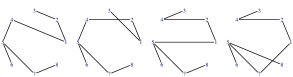
Figure 4. A walk using only quadratic moves from $g_{1}$ to $g_{2}$ on the fiber $\mathcal{F}_{(2,1,1,2,3,1,2,1)}$.

The commutative algebra community has known the structure of these generators, without calling them moves or relating them to MCMC methods, for at least 20 years, for example, in [Vil95, Vil00] and [OH99], as well as [Stu96, Chapter 9] and [RTT12].

Further, these results have been known in the algebraic statistics literature for some time as well. Notable examples include works such as [SS06, Theorem 4] on toric geometry of compatible full conditionals, [Mor13, Theorem 3.2] on relations among conditional probabilities, [SW12] that studies algebra and geometry of statistical ranking models and the ascending model in particular, and [PRF10] that study the structure of Markov and Graver bases for the directed model $p_{1}$ whose restriction (to the part of the random graph consisting only of reciprocated edges) is the $\beta$ model. More recently, [OHT13] offer the exact test implementation whose main ingredient is a random generation of Markov and Graver bases elements for the $\beta$ model.

Interestingly, bicolored or alternating closed walks on graphs make a later appearance in computer science literature as well. [BPS09] define the alternating cone of a graph to be the set of characteristic vectors of alternating walks on the graph, cf. [BPS07] and the subsequent book chapter [Bha12]. In algebraic terms, this is the cone of exponent vectors of the binomials in the toric ideal of that graph. Results from toric algebra of graphs and the definition of the alternating cone should easily imply that [BPS09, Conjecture 3.1] is actually true, and can furthermore be generalized for hypergraphs appropriately. [Sri] is a very nice set of notes on open problems related to threshold graphs; cf. Conjecture 4. To prove the conjecture, note that a ‘balanced sum of cycles’ is certainly a balanced graph, thus it is a lattice point in the cone of balanced subgraphs. Each of these lattice points is an integer exponent of some binomials in the toric ideal of the graph. It is well known that the Graver basis is an integral generating set of the lattice, in that every lattice point in the cone can be written as a integral sum of the Graver exponents. Finally, Graver bases of these cones for graphs are encoded by alternating walks by [Vil95], see also recent literature cited above. More generally, for hypergraphs, the walks are interpreted as bi-colored [PS14] and again form a Graver basis; see [PTV] for the general non-uniform case. By definition, these are exactly balanced subgraphs. Thus, the exponent vector of a balanced sum of cycles is an integral sum of balanced subgraphs represented by Graver elements. The present author is not aware of whether the conjecture has been proved in other literature; only the fractional sum part of the conjecture is proved in the works on alternating cones cited above.

Apart from the $\beta$ model for random graphs, sampling algorithms for the space of graphs with fixed properties have evolved disjointly from statistics. At this point, solutions to the following two subproblems of Problem 3.1 are of special importance:

Problem 3.6 (An instance of General Problem 1: $p_{1}$ model moves).

Determine a set of moves sufficient to connect the space of graphs, consisting of both directed and bidirected (reciprocated) edges, with a given directed degree sequence and number of reciprocated edges.

The problem above was solved in algebraic statistics [PRF10] and an implementation of a dynamic algorithm was offered in [GPS]; see the subsection on mixing times below for a related open problem.

Problem 3.7 (An instance of General Problem 1: Hypergraph $\beta$ model moves).

Determine a set of moves sufficient to connect the space of hypergraphs, uniform, layered or general, with a given degree sequence.

Of course, one can ‘solve’ these problems in various ways. From the point of view of (algebraic) statistics applied to networks, the most interesting types of solutions to Problems 3.7 and 3.1 in general will at least address general models with sampling constraints and forbidden edges, or derive bases of bounded complexity with good mixing time properties for a subclass of the models. The literature offers some examples of such solutions, but many problems remain open. These issues are discussed next.

Sampling constraints

If, in applications, the random sampler of the model fibers is allowed to step through the extended state space of non-simple graphs, where edges can have a multiplicity, then the problem is solved. For example, simple-edge-swap solution to Problem 3.7 follows from standard textbook results in algebraic geometry; namely, the generating set of the toric ideal for the model is known to consist of quadratic binomials, as the algebraic closure of the model is defined by the toric ideal of the second hypersimplex, known to be generated by quadrics. However, inherent sampling constraints can compound the issue of computing a set of moves guaranteed to connect each fiber, for example, the sampler may need to step through only simple graphs, or graphs with bounded multiplicity. In some statistical modeling considerations other constraints may come in the form of forbidden edges or forbidden neighbors; such constraints in statistics are called structural zeros of the model. Of course sampling and modeling constraints restrict the fiber, as expected, but also make the required moves more complicated: consider the situation when the edges used in the intermediate steps of the walk in Figure 4, such as the edge $\{1,3\}$ for example, are structural zeros.

Interestingly, [HTE⁺09] characterize when a sequence is realizable as a degree sequence of a simple graph such that a given set of edges from an arbitrary node is avoided. This allows the authors to construct a swap-free algorithm for sampling the restricted fiber of the $\beta$ model. If one is interested in sampling a restricted fiber for any general linear ERGM or any log-linear model, [OHT13] and [AHT12] show that one needs a much larger set of moves to guarantee connectivity, i.e. minimal Markov bases may not do the job. For example, the set known to algebraists to be inherently more complicated, called the Graver basis of the toric ideal [DSS09, §1.3], [AHT12, §4.6] will suffice to connect the fiber, however it is also so complex and large that it is not feasible to compute it for any reasonable example beyond toy-size networks; to give an idea of such size, for the $p_{1}$ model this basis can only be directly computed for networks on less than 7 nodes. What [OHT13] then do is provide an algorithm that constructs one step in the chain – a Markov move – in a dynamic fashion and show its performance on several small network datasets. Since the moves generated belong to the Graver basis, the method is provably applicable in the case of structural zeros and sampling constraints. This method does rely on the understanding of the algebraic machinery underlying the model, but appears to be inefficient in discovering the fiber and the resulting Markov chain has a high rejection rate. In contrast, simulations indicate that the chain from [GPS, §4.1] does not have that problem, but there is no formal proof of its good properties. This leads us to the next topic regarding sampling fibers.

Mixing time considerations

Considerations of mixing times/convergence are crucial in any MCMC sampling scheme [RC09] [BGJM11]. Notably, using minimal Markov bases may not produce good mixing as seen in some experiments and pointed out recently in [Win], which formalizes how mixing properties of Markov bases depend on the structure and connectedness in particular of the underlying fiber graph. Moreover, it explains that results on mixing times of chains built on minimal Markov bases are in general prohibitive to obtain, and suggests instead the construction of related expander graphs for the problem - a worthwhile pursuit. In earlier work, [GPS] construct a chain on the fiber graph for the $p_{1}$ model in in such a way that it is, in fact, a complete graph, with loops having seemingly low probability. In simulations, the chain behaves quite well and indicates fast mixing. Nevertheless, a formal proof of rapid mixing or any mixing properties are left as open questions, as the authors there did not study the structure of the transition matrix for that chain.

This is where recent advances in discrete literature, for some reason disjoint from statistics literature on networks, offer example results for the $\beta$ model that, in this author’s opinion, should be connected to statistics - algebraic statistics in particular - and used as a guide for studying Markov bases of other linear and general ERGMs. Namely, [KTV99] conjectured that the Markov chain based on swaps mixes rapidly, and the proofs for arbitrary regular graphs and half-regular bipartite graphs were given in [CDG07] and [MES13], respectively, while irregular graphs are studied in [Gre15]. Recently, [EMT15] offer insight to the general case via the study of swap-based chains on the fibers of the JDM model from Example 2.2; they prove fast mixing on a subset of the JDM-model fibers and offer an excellent review of related literature, while irreducibility of the Markov chain on the JDM realizations was proved in [CDEM15]. To translate what this means for Markov bases, note that in algebraic statistics language, ‘swaps’ of two edges at a time are quadratic Markov moves, or quadratic generators of the toric ideal, since taking two edges at a time and replacing them by two other edges translates to a quadratic monomial in Example 3.4.

Crucially, however, the difference is not just linguistic: in general in algebraic statistics, Markov moves are sampled from a set of all possible moves that apply to the model, that have been computed a priori. Such sampling can clearly lead to more rejections. On the other hand, ‘swaps’ are constructed from observed edges, so rarely is a non-applicable swap proposed! In particular, the literature cited here provides a set of examples of rapidly mixing sequences of fiber graphs, and thus also hope that Markov-move-based constructions, adapted appropriately, can still lead to good chains for fiber exploration and goodness-of-fit tests; compare to examples reported in [GPS] or [OHT13] for an illustration.

In the remainder of this subsection, let us clarify how these chains should be constructed ‘with care’, and why an out-of-the-box Markov basis may not be good enough. For example, [Win] observes that enlarging minimal Markov bases to, say, Graver bases doesn’t improve mixing time. Intuitively, if the chain can be constructed so that the fiber graph has a relatively small number of loops, then rapid mixing may be possible. Such a fiber graph would resemble the idea of using moves corresponding to graph-theoretic ‘swaps’: namely, not attempting to construct or apply Markov moves that work on just some fiber, but, instead, focus on the given observed graph and its particular fiber. We refer to such moves as data-dependent. Incidentally, the chain on the $p_{1}$ model used a large set of moves that is guaranteed to contain the Graver bases in combination with constructing data-dependent moves dynamically, involving both ‘large’ and ‘small’ steps on the fibers of the $p_{1}$ and $\beta$ models, shows excellent mixing properties in simulations on networks of various sizes. In fact, the Graver move from Figure 3 was constructed using the particular implementation from [GPS], without going through the intermediate steps in Figure 4. In the language of Example 3.5, what we construct is a random walk on the realizable lattice points of the alternating cone using a superset of the Graver basis for the toric ideal of the complete graph, or for an arbitrary graph whose missing edges represent structural zeros in the $p_{1}$ model. This leads us to the final remark about Markov bases construction, which is intimately related to mixing time, but deserves to be singled out.

Data-dependent samplers

That knowing an entire Markov basis for a model may still not be sufficient to run goodness-of-fit tests efficiently is a well-known fact in algebraic statistics. Namely, Markov bases are data-independent [DFR⁺08, Problem 5.5]. To paraphrase [AHT12]: since a Markov basis is common for every fiber, the set of moves connecting the particular fiber of the observed data will usually be significantly smaller than the entire basis for the model. The subsequent paper [Win] offers another intuitive explanation of why data-dependent fiber samplers are necessary: “The conclusions we draw […] are that an adaptation of the Markov basis has to take place depending on the right-hand side”, meaning that distinct fibers require different adaptations, confirming previous observations. To handle precisely this issue, [Dob12] suggested generating only moves needed to complete one step of the random walk, and then covering the fiber by sets of local moves; this was the first scalable method for exact tests on tables beyond decomposable models [DS04] and applicable to log-linear models where sufficient statistics are table marginals. However, many models of interest are not captured by marginals [SZP14, HL81, KPP⁺, GZFA09], leaving a gaping hole in the methodology for other categorical models, particularly for sparse data. This leads us to consider more general models for networks, with a long-term aim to design a data-dependent sampler beyond the one in [GPS] and [OHT13] for the $p_{1}$ and $\beta$ models.

3.2. General linear ERGMs

The situation may now seem hopeless for general non-degree-based models, because even if we establish fast mixing for Markov chains on $\beta$ model fibers, there are infinitely many other models that are left to be considered. However, not all is lost: it turns out that as long as the model is log-linear and the sufficient statistics are given by a linear map from the sample space, sampling hypergraphs with prescribed degree sequences, uniform or not, and with prescribed forbidden edges actually suffices for performing the exact test. This takes care of a number of interesting models! The answer lies in the structure all log-linear models including linear ERGMs: each of these models is encoded by a hypergraph, defined in [PS14], Section 3.1 of which provides further details and a simple example for the independence model.

Definition 3.8.

The parameter hypergraph $\mathcal{H}_{\mathcal{M}}$ of any log-linear model $\mathcal{M}$ for discrete data, and any linear ERGM in particular, is the hypergraph whose vertex set $\theta_{1},\dots,\theta_{n}$ corresponds to the parameters of the statistical model, and whose edge set is determined by joint probabilities of all possible states of the random variables $Z_{1},\dots,Z_{m}$. More precisely, $\{\theta_{j}\}_{j\in J}$ is an edge in the parameter hypergraph if the index set $J$ describes one of the probabilities in the model, that is, there exist values $i_{1},\dots,i_{m}$ such that $Prob(Z_{1}=i_{1},\dots,Z_{m}=i_{m})=\prod_{j\in J}\theta_{j}$.

Example 3.9.

Let $\mathcal{M}_{\beta}$ be the $\beta$ model for random graphs on $n$ vertices $v_{1},\dots,v_{n}$. The parameter hypergraph $\mathcal{M}_{\beta}$ is the complete graph on vertices $\beta_{1},\dots,\beta_{n}$. To see why, recall the probability formula of the edges in Example 2.1: the random variables $Z_{1},\dots,Z_{m}$ represent the $m={n\choose 2}$ edges of the graph. The probability of the joint state where $Z_{k}=1$ and $Z_{l}=0$ for $l\neq k$, that is, the event of the occurrence of only the edge $Z_{k}:=\{i,j\}$ in the graph, is proportional to $\beta_{i}\beta_{j}$. Note that $\mathcal{H}_{\mathcal{M}}$ being complete does not mean that all edges $\{v_{i}v_{j}\}$ in the random graph are observed, but instead that all edges $\{\beta_{i}\beta_{j}\}$ of $\mathcal{M}_{\beta}$ correspond to random graph edges that are allowed. In particular this is why the graph on the right of Figure 2 is complete with non-zero probability weights on every edge- there are no structural zeros in that example.

Similarly, for the hypergraph $\beta$ model, the parameter hypergraph is the complete hypergraph, either uniform, layered, or general, respectively in each of the there cases of the model. Recently, the hypergraph $\mathcal{H}_{p_{1}}$ of the $p_{1}$ random graph model was described in [GPS] and consists of edges of sizes 1, 3 and 7, for probabilities of no connection between two nodes, or a directed edge, or a reciprocated edge, respectively; for example, a directed edge $i\rightarrow j$ occurs with probability $\lambda_{ij}\alpha_{i}\beta_{j}$ and is thus encoded by a $3$-edge on $\mathcal{H}_{p_{1}}$.

Remark 3.10.

The parameter hypergraph runs the danger of being lost in translation, so to understand its construction, recall that the sufficient statistics of $\mathcal{M}$ are computed using a linear map. Let $M$ be the matrix of that linear map. The parameter hypergraph $\mathcal{H}_{\mathcal{M}}$ of the model is simply the hypergraph whose vertex-edge incidence matrix is this matrix $M$.
For the $\beta$ model, the definition may appear trivialized, but further log-linear model examples show this isn’t the case in general; see for example Figure 2 in [GPS] for two further examples of parameter hypergraphs.

What about the fibers of $\mathcal{M}$? Consider again the $\beta$ model for graphs: two random graphs $g_{1}$ and $g_{2}$ occur with the same probability and are in the same fiber of the model if and only if their images under the linear map $M$ are the same. If $g_{1}$ and $g_{2}$ are encoded by a set of red and blue edges on $\mathcal{M}_{\beta}$, respectively, they have the same probability if and only if the same multiset of parameters $\beta_{i}$’s are covered by the red and blue edges. In other words, the red edge set and the blue edge set are graphs with the same degree sequence. This degree sequence correspondence for $\mathcal{M}_{\beta}$ seems trivial; remarkably, it holds for all linear ERGMs.

Definition 3.11.

Let $E$ be a multiset collection of edges in a hypergraph $H$. $E$ is balanced with respect to a given bicoloring of $H$ if for each vertex $v$ covered by $E$, the number of red edges containing $v$ equals the number of blue edges containing $v$. In other words, the ‘blue degree’ of $E$ equals its ‘red degree’.

The definition above appears as Definition 2.7 in [PS14] for the case of uniform hypergraphs, and Definition 5.7 in [PTV] for an arbitrary hypergraph. The motivation for this definition and interpretation of the binomials as bicolored edge sets was to study toric algebra of hypergraphs by generalizing the algebraic literature on graphs. The bicoloring construction idea simply generalizes Villarreal’s [Vil95] ‘closed alternating walks’ on graphs, see [RTT12] for a further classification and characterization of the walks. A straightforward argument now shows the following.

Theorem 3.12 (See Theorem 2.8 of [PS14] for the uniform case).

Let $\mathcal{H}_{\mathcal{M}}$ be the parameter hypergraph of the model $\mathcal{M}$. Then any balanced collection of edges $E\subset E(\mathcal{H})$ constitutes a move in the toric ideal associated to $\mathcal{H}$. In particular, the set of balanced bicolored subgraphs connect all fibers of the model $\mathcal{M}$.

Note that a balanced bicolored hypergraph is simply a set of two hypergraphs, not necessarily simple, that have the same degree sequence! Examples and structure of balanced edge sets on a hypergraph, as well as extension to the non-uniform case, can be found in [PTV, §5.1 and 5.2].

Thus far, we have seen how all linear ERGMs that are encoded by $0/1$ matrices $M$ - ‘legal’ incidence matrices - give rise to parameter hypergraphs. But what about models whose probability form is more general? Surprisingly, by a recent result [PTV, Theorem 6.2], all toric ideals and therefore all linear ERGMs and log-linear models for discrete data are such that there exists a hypergraph that encodes their Graver bases and preserves the complexity. Therefore, we arrive at the following crucial fact:

The parameter hypergraph encodes sufficient statistics of any linear ERGM by a hypergraph degree sequence.

This further reinforces the present author’s view that discrete mathematics literature on sampling graphs and hypergraphs with fixed properties should be imported to statistics and considered a crucial tool in linear ERGM model fitting in particular. The following General Problem summarizes the discussion of this section:

Problem 3.13 (A restatement of General Problem 1 with constraints).

Fix a general linear ERGM with model hypergraph $\mathcal{H}$, so that the incidence matrix of $\mathcal{H}$ computes the sufficient statistics vector $T(g)$ for the random graph $g$. Develop an efficient algorithm that samples from the set of sub-hypergraphs of $\mathcal{H}$ with arbitrary fixed degree sequence.

Of course, as discussed above, we know that ‘2-switches’, or quadratic Markov moves, suffice to connect all realizations of hypergraph degree sequences because they correspond to the the defining ideal of the variety of Veronese-type corresponding to the r-th hypersimplex [Stu96, Chapter 14], but intermediate steps may go through non-simple hypergraphs, that is, those that have edges with multiplicities larger than $1$. Further, this construction ignores possible forbidden edges. A related problem for the restricted class of complete $k$-uniform hypergraphs can be found in the problem collection [Wes, Problem 2]: For $k\geq 4$, determine whether there exists a function $f(k)$ and a set of operations, each on at most $f(k)$ vertices, that can be used to transform one $k$-realization of a $k$-graphic sequence into another. Even if this problem is solved, it would only impact the uniform case of the hypergraph $\beta$ model, for which $\mathcal{H}_{\mathcal{M}}$ is complete, that is, there are no forbidden edges. For applications, statistical sampling constraints and forbidden edges really impact the solution. For example, the famous ‘bad news Theorem’ for Markov bases in algebraic statistics from [DLO06] shows that Markov bases for already the simplest non-trivial model on $3$ discrete random variables, called the no-three-way interaction model, are arbitrarily complicated. What this means is that there are fibers of observable data points that require moves of arbitrarily large degree if the number of states of at least two of the $3$ variables are not bounded. For completeness, let me add also the complementing ‘good news Theorem’ for Markov bases famous in algebraic statistics: [HS07] show that the Markov bases for that same no-three-way interaction model have bounded complexity if the number of states of two of the $3$ variables is bounded. Incidentally, the parameter hypergraph of the no-three-way model is $3$-uniform and $3$-partite, it is not complete: there are as many edges as in $K_{p,q}$ where $p$ and $q$ are sizes of two of its parts, and it is regular in each part. So the presence of forbidden edges in $\mathcal{H}_{\mathcal{M}}$ compound the issue of connecting the fiber in the worst possible way. However, positive results can be obtained for restricted classes of problems, references to which are scattered throughout this section.

4. Polytopes play an important role in ERGMs

The parameter estimation problem

In the estimation problem, given an observation of the joint states of the random variables, the goal is to estimate the unknown probability distribution $p_{\theta_{0}}$ from a model $\mathcal{M}$ that ‘best explains’ the data. A basic method commonly used is that of maximum likelihood estimation: a maximum likelihood estimate (MLE) of $\theta_{0}$ is a parameter vector $\hat{\theta}\in\Theta$ that makes the given data most likely to have been observed. It is defined as:

(4.1) $$\widehat{\theta}=\mathrm{argmax}_{\theta\in\mathbb{R}^{n}}p_{\theta}(x).$$

Computing it amounts to maximizing the log-likelihood function, which maps the parameters indexing the probability distributions in a model to the likelihood of observing the given data. While there are several estimators that can be used, an MLE is a very straightforward one that enjoys nice statistical properties such as consistency and asymptotic efficiency, and computing it is a seemingly simple optimization problem. However, there are several obstacles. One if them is that the MLE of the natural parameters of the model may not exist, meaning that we are unable to make inferences about any or a subset of the parameters from the given data. As expected, the estimation problem has been studied in detail in the statistics literature for many classes of models. In the last decade, it has been shown that for discrete exponential families, the geometric structure of the model captures important information about parameter estimation including MLE existence; see [RFZ09], [DFR⁺08], cf.  [Gey09], [Han03]. Luckily, in case of exponential families, if the MLE exists it is unique. The following polyhedral object captures the MLE information in exponential family models.

Definition 4.1.

Let $\mathcal{T}=\{T(g)\in\mathbb{R}^{d}\}$ be the range of sufficient statistics $T$, where $g$ ranges over the set of all observable networks in the sample space. The model polytope associated with the family $\mathcal{M}$ is

$$\mathrm{P}=\mathrm{convhull}(\mathcal{T})\subset\mathbb{R}^{d}.$$

We may assume $P$ to be full-dimensional.

Example 4.2.

The model polytope $\mathrm{P}$ for the $\beta$ model for random graphs on $n$ vertices is the polytope of degree sequences of graphs on $n$ vertices. [RPF13] use the explicit description of facets from [MP95] to give a characterization of when the sufficient statistic vector is on the boundary of the polytope, and study the statistical consequences.

The complexity of the MLE problem for the model $\mathcal{M}$ is captured by the geometry of the polytope $\mathrm{P}$ and by the combinatorics of its face lattice as follows: the MLE for the observed data exists if and only if the observed sufficient statistic vector lies in the relative interior of the model polytope $\mathrm{P}$. For instance, [RPF13] studies MLE existence for the $\beta$ model for graphs and links to the graph theory literature on degree sequences. Nonetheless, partly because the link with polyhedral geometry has remained largely unexplored in both the mathematical and statistical literature, methodologies for estimation and model validation under a non-existent MLE with proven statistical performance have yet to be developed. A first step in this direction is to solve the following.

Problem 4.3 (General Problem 2).

Fix a random graph model with sufficient statistics vector $T(g)$ and sample space $\mathcal{G}_{n}$. Often, $\mathcal{G}_{n}$ will be the set of simple graphs on $n$ vertices. Determine the model polytope $P=conv\{T(g):g\in\mathcal{G}_{n}\}$. What are the extreme points? What is the facial structure? What is the proportion of realizable lattice points on the boundary vs. in the interior?

The following can be thought of a subproblem of 4.3, but due to its difficulty and relevance for developing algorithms to detect MLE non-existence, we single it out.

Problem 4.4 (A sequel to General Problem 2).

Develop an efficient algorithm that can determine whether a given point lies on the relative interior of $P$; i.e., obtain a facet description of the model polytope that is ‘efficient’.

While the general theoretical link between statistical estimation and polyhedral geometry is in place for discrete exponential families as outlined in [RFZ09] and references therein, statistics now relies on discrete methods to provide the required tools. Let us gather here some of the relevant results. We emphasize again that for discrete exponential families if an MLE exists then it is unique. Estimation algorithms will behave well when off the boundary of the polytope. For example, [SSR⁺14] define the hypergraph $\beta$ model and show that fixed point algorithms will converge to the MLE geometrically fast as long as the sufficient statistic is on the relative interior of the polytope. [RPF13] use the polytope of graphical degree sequences to offer a complementary study to [CDS11] of the estimation problem in the $\beta$ model. Another simple of interest is called the edge-triangle model. Its sufficient statistic vector consists of two numbers: the number of edges and the number of triangles in the graph. Its polytope and estimation issues are addressed in [RFZ09], the asymptotics of the MLE existence problem, polytope and its fan in [YRF13], while [HCT15] study its degeneracy from the point of view of statistical mechanics, dealing with the issue of non-realizable points that exist within the model polytope in such a way that they are meant to represent data averages but are by definition non-interpretable.

However, Problem 4.3 has not been solved for most models listed in this review. For example, the polytope of hypergraph degree sequences has been studied in the literature and some partial results are known: [Liu13] shows that the set of hypergraph degree sequences for uniform hypergraphs is non-convex, and thus Erdös-Gallai-type theorems do not hold. [MS02] also offers a very nice review of the problem, and shows that vertices of the polytope are known by Theorem 2.5. Namely, they are $r$-threshold sequences, where $r$ is the uniformity of the hypergraph. Further, some of the facet inequalities are known.

Data privacy and noisy sufficient statistics

Statistical analyses of network data sometimes require projection of a noisy degree sequence onto the model polytope, in particular its realizable points. The noisy sequence need not be a realizable degree sequence vector at all. The example below is considered from the point of view of data privacy and confidentiality, but note that the problem is also relevant for noisy sampling, for example when there are measurement errors and the reported observed sufficient statistic does not represent a realizable sequence.

The basic concept of data privacy and confidentiality is to minimize the risk of releasing sensitive information about, say in our case, people in a social network, while maximizing statistical utility of the data. Having statistical utility means that the released information can be used for statistical analyses. A straightforward example of such information that one may want to release is the observed value of the sufficient statistic. However, in the age where information about any particular data set may be gathered from different sources, releasing a sufficient statistic, e.g., the degree sequence in the $\beta$ model case, may not be ‘private enough’. For this reason, in the interest of preserving data privacy, noise is added to the observed sufficient statistic in order to have it releasable to the public while not jeopardizing sensitive network information. Of course this presents various problems for statistical inference; thus the noise is added in a principled way. There are several well-known privacy-preserving mechanisms. The statistical task is then to determine how to perform reliable inference using the noisy statistic; for an example and overview of the relevant privacy literature for ERGMs see [SKK14]. One of the steps in [KS16] that is required for computing a private parameter estimator of the released data, with good statistical properties, is to project the noisy sufficient statistic onto the lattice points in the model polytope. To this end, one needs to understand the following.

Problem 4.5 (General Problem 3).

Fix a random graph model with sufficient statistics vector $T(g)$, sample space $\mathcal{G}_{n}$. Often, $\mathcal{G}_{n}$ will be the set of graphs on $n$ vertices. Let $P=conv\{T(g):g\in\mathcal{G}_{n}\}$ be the model polytope. Develop an (efficient) algorithm to compute the projection of a noisy sufficient statistic vector onto the realizable vectors in $P$.

Obviously, determining if a lattice point is a realizable sufficient statistic for the model $\mathcal{M}$ is a problem on its own. In fact realizability results of Havel-Hakimi [Hav55, Hak62] type can be used to solve Problem 4.5:

Example 4.6.

For the $\beta$ model, [KS16, KS12] use the Havel-Hakimi decomposition to compute the realizable lattice point in the polytope of degree sequences that is closest to the given noisy sequence. In order to achieve a more efficient implementation, they in fact use the polytope of degree partitions [BSS06], that is, of sorted degree sequences. This polytope can be thought of as an asymmetrized version of the degree sequence polytope.

This directly leads to the analogous problems for the other models, which are singled out for convenience.

Problem 4.7 (An instance of General Problem 3).

Generalize Havel-Hakimi to the $p_{1}$ model polytope.

Remarkably, the directed part of this problem has been solved in [EMT10], where they also study the case of some forbidden edges. The authors there also prove a result useful to design an MCMC algorithm to find random realizations of prescribed directed degree sequences, which relates back to Problem 3.6 (solved in [PRF10]). However, this sampling algorithm offers a partial solution to the problem in the general case, though it should be easy to modify it to fit the statistics framework. Namely, in the general variant of the $p_{1}$ model, reciprocated edges are of the form $i\rightarrow j$ and $i\leftarrow j$ simultaneously combined into one bidirected edge $i\leftrightarrow j$. The sufficient statistics of the $p_{1}$ model include the number of reciprocated edges! This means that in sampling or finding random realizations, this number also matters: reciprocated edges are allowed to be ‘pulled apart’ while sampling, but the total number of them is to remain constant. Recall again that forbidden edges in this case correspond to structural zeros in the $p_{1}$ model.

Problem 4.8 (An instance of General Problem 3).

Generalize Havel-Hakimi to the three variants of the $\beta$ hypergraph model polytope: uniform, layered or general hypergraph degree sequences.

The uniform instance of this problem is essentially [BEF⁺13, Problem 1.1], who also emphasize that the only known characterization of $k$-graphic sequences is due to Dewdney in 1975, but it does not yield an efficient algorithm. Two of the variants of the $\beta$ hypergraph model work with nonuniform hypergraphs.

5. Concluding remarks

There exist, of course, families of ERGMs beyond the ones discussed in this brief overview, including those based on global summary statistics not related to node degrees, for example the cores decomposition [KPP⁺], or other types of models such as graphical models for networks [SR14a]. A uniform sampler for the fibers of the former model family has not been developed, while the algebra and geometry of the latter model family has not been explored. Clearly these are interesting problems in the statistical analysis of networks and, in particular, algebraic statistics. But the main points of this chapter are:

• Several basic examples of linear ERGMs already offer many interesting open problems in discrete mathematics, instances and special cases of which are already known and interesting in their own right from the graph-theoretic point of view.

• These models also provide a theoretical foundation for exploring distributions of various network summary statistics that could serve to develop a rigorous testing and model fitting framework for networks, nowadays generally lacking despite the exploding literature on network analysis.

The first type of problem discussed here is the sampling problem given a fixed set of characteristics of a network. Within the context of statistical modeling of networks, the value of sampling and therefore of exact testing can be summarized as follows. Comparing to the reference set $\mathcal{F}_{t}$ avoids the use of asymptotics, offers an alternative to model fit testing, and makes it unnecessary to use large-sample approximations to sampling distributions, in particular when their adequacy has not been determined. As demonstrated on several cases in the literatue, tools from algebraic statistics offer a valid and critical approach for analyzing such models. However, within this realm of mathematical research, several problems remain, including problems related to scalability and applicability of the algebraic methods. The second type of problem discussed here is related to the model polytope defined to be the convex hull of all sufficient statistics for the model. The polytope captures the difficulty of parameter estimation and MLE existence and is a crucial step in statistical inference. Both problems are key steps in the general scheme of testing goodness of fit of the model and model selection, detailed statistical considerations of which are beyond the scope of the present chapter.

To close, it is worth pointing out that algebraic statistics is in fact a much broader field, not confined to the study of log-linear models for discrete data. Indeed, the field builds upon the rich and long history of the use of algebraic tools in statistics, starting with Fisher [Fis25] and algebra for confounding [PW83], but has expanded to encompass at least three distinct fields of mathematics: commutative and computational algebra, via solving systems of polynomial/rational equations; combinatorics of graphs, hypergraphs, and simplicial complexes; and geometry, algebraic, convex, and polyhedral. The field is roughly two decades old, yet it has many facets, and recent theoretical advances show that there is a significant impact on applicability and behavior of various statistical methods, including but not limited to the following problems: parameter estimation and reliability of inference for discrete exponential families [RFZ09, RPF10] and Gaussian models [ZUR]; general methods for experimental design [PRW01]; parameter identifiability studied in numerous references of [APRS11], [FSD11] and complexity of parameter estimation for Gaussian graphical models [DFD12], [DGP12], [GS]; Bayesian model selection and singular learning theory [Wat10, Wat09], sampling from conditional or marginal distributions on contingency tables with implications to cell bounds and data privacy [Sla10, SZP14], exact tests for marginal table models [Dob03], and model fitting via exact tests for degree-based network models [OHT13, SSR⁺14], as well as offering new models and algorithms for networks not based on degrees [KPP⁺]. This bibliography is far from complete, but should give enough information on some recent advances in the field to the interested reader.

References

- [Agr92] Alan Agresti, A survey of exact inference for contingency tables, Statistical Science 7 (1992), no. 1, 131–153.
- [AHT12] Satoshi Aoki, Hisayuki Hara, and Akimichi Takemura, Markov bases in algebraic statistics, Springer Series in Statistics, Springer New York, 2012.
- [APRS11] Elizabeth Allman, Sonja Petrović, John Rhodes, and Seth Sullivant, Identifiability of two-tree mixtures under group-based models, IEEE/ACM Transactions in Computational Biology and Bioinformatics 8 (2011), no. 3, 710–722.
- [BD10] Joseph Blitzstein and Persi Diaconis, A sequential importance sampling algorithm for generating random graphs with prescribed degrees, Internet Math 6 (2010), 489–522.
- [BD15] Peter J. Bickel and Kjeli A. Doksum, Mathematical statistics, basic ideas and selected topics, vol. 1, 2 ed., Chapman & Hall/CRC Texts in Statistical Science, 2015.
- [BDE] Michael J. Bannister, William E. Devanny, and David Eppstein, ERGMs are Hard, Preprint, arXiv:1412.1787 [cs.DS].
- [BEF+13] Sarah Behrens, Catherine Erbes, Michael Ferrara, Stephen G. Hartke, Benjamin Reiniger, Hannah Spinoza, and Charles Tomlinson, New results on degree sequencesof uniform hypergraphs, Electronic Journal of Combinatorics 20 (2013), no. 4.
- [BGJM11] Steve Brooks, Andrew Gelman, Galin L. Jones, and Xiao-Li Meng (eds.), Handbook of Markov Chain Monte Carlo, Handbook of Modern statistical methods, Chapman & Hall/CRC, 2011.
- [Bha12] Amitava Bhattacharya, Alternating reachability and integer sum of closed alternating trails, Graph-Theoretic Concepts in Computer Science: 38th International Workshop WG 2012 (Martin Charles Golumbic, Michael Stern, Avivit Levy, and Gila Morgenstern, eds.), Lecture Notes in Computer Science, Springer, 2012.
- [BN14] Ole Barndorff-Nielsen, Information and exponential families in statistical theory, Wiley, 1978, reprinted in 2014.
- [BPS07] Amitava Bhattacharya, Uri Peled, and Murali K. Srinivasan, Cones of closed alternating walks and trails, Linear Algebra and its Applications 423 (2007), no. 2-3, 351–365.
- [BPS09] by same author, The cone of balanced subgraphs, Linear Algebra and its Applications 431 (2009), no. 1-2, 266–273.
- [Bro86] Lawrence Brown, Fundamentals of statistical exponential families, Monograph Series, vol. 9, IMS Lecture Notes, Hayward, CA, 1986.
- [BSS06] Amitava Bhattacharya, Sivaramakrishnan Sivasubramanian, and Murali K. Srinivasan, The polytope of degree partitions, Electronic Journal of Combinatorics 13 (2006), no. 1.
- [CDEM15] Éva Czabarka, Aaron Dutle, Péter L. Erdös, and Istvan Miklós, On realizations of a joint degree matrix, Discrete Applied Mathematics 181 (2015), 283–288.
- [CDG07] Colin Cooper, Martin Dyer, and Catherine Greenhill, Sampling regular graphs and a peer-to-peer network, Combinatorics, Probability and Computing 16 (2007), no. 4, 557–593.
- [CDS11] Sourav Chatterjee, Persi Diaconis, and Allan Sly, Random graphs with a given degree sequence, Ann. Appl. Probab. 21 (2011), no. 4, 1400–1435.
- [CKHG15] Nicole Bohme Carnegie, Pavel N. Krivitsky, David R. Hunter, and Steven M. Goodreau, An approximation method for improving dynamic network model fitting, Journal of Computational and Graphical Statistics 24 (2015), no. 2, Journal of Computational and Graphical Statistics, in press.
- [DFD12] Mathias Drton, Rina Foygel, and Jan Draisma, Half-trek criterion for generic identifiability of linear structural equation models, Annals of Statistics 40 (2012), no. 3, 1682–1713.
- [DFR+08] Adrian Dobra, Stephen E. Fienberg, Alessandro Rinaldo, Aleksandra Slavković, and Yi Zhou, Algebraic statistics and contingency table problems: Log-linear models, likelihood estimation and disclosure limitation., In IMA Volumes in Mathematics and its Applications: Emerging Applications of Algebraic Geometry, Springer Science+Business Media, Inc, 2008, pp. 63–88.
- [DGP12] Mathias Drton, Elizabeth Gross, and Sonja Petrović, Maximum likelihood degree of variance component models, Electronic Journal of Statistics 6 (2012), no. 0, 993–1016.
- [DLO06] Jesus A. De Loera and Shmuel Onn, Markov bases of three-way tables are arbitrarily complicated, J. Symbolic Comput. 41 (2006), no. 2, 173–181.
- [Dob03] Adrian Dobra, Markov bases for decomposable graphical models, Bernoulli 9 (2003), no. 6, 1093–1108.
- [Dob12] by same author, Dynamic Markov bases, Journal of Computational and Graphical Statistics (2012), 496–517.
- [DS98] Persi Diaconis and Bernd Sturmfels, Algebraic algorithms for sampling from conditional distributions, Annals of Statistics 26 (1998), no. 1, 363–397.
- [DS04] Adrian Dobra and Seth Sullivant, A divide-and-conquer algorithm for generating Markov bases of multi-way tables, Computational Statistics 19 (2004), 347–366.
- [DSS09] Mathias Drton, Bernd Sturmfels, and Seth Sullivant, Lectures on algebraic statistics, Oberwolfach Seminars, vol. 39, Birkhäuser, 2009.
- [EMT10] Péter L. Erdös, Istvan Miklós, and Zoltán Toroczkai, A simple Havel–Hakimi type algorithm to realize graphical degree sequences of directed graphs, Electronic Journal of Combinatorics 17 (2010), no. 1.
- [EMT15] by same author, A decomposition based proof for fast mixing of a markov chain over balanced realizations of a joint degree matrix, SIAM Journal of Discrete Math 29 (2015), no. 481-499.
- [Fis25] Sir Ronald Aylmer Fisher, Statistical methods for research workers, Edinburgh: Oliver & Boyd, 1925.
- [FMW85] Stephen E. Fienberg, Michael M. Meyer, and Stanley S. Wasserman, Statistical analysis of multiple sociometric relations, Journal of the American Statistical Association 80 (1985), 51–67.
- [FSD11] Rina Foygel, Seth Sullivant, and Mathias Drton, Global identifiability of linear structural equation models, Annals of Statistics 39 (2011), 865–886.
- [FW81] Stephen E. Fienberg and Stanley S. Wasserman, Discussion of Holland, P. W. and Leinhardt, S. “An exponential family of probability distributions for directed graphs.”, Journal of the American Statistical Association 76 (1981), 54–57.
- [Gey09] Charles J. Geyer, Likelihood inference in exponential families and directions of recession, Electronic Journal of Statistics 3 (2009), 259–289.
- [Goo07] Steven M. Goodreau, Advances in exponential random graph () models applied to a large social network, Social Networks 29 (2007), no. 2, 231–248.
- [GPS] Elizabeth Gross, Sonja Petrović, and Despina Stasi, Goodness-of-fit for log-linear network models: Dynamic Markov bases using hypergraphs, Annals of the Institute of Statistical Mathematics, to appear.
- [Gre15] Catherine Greenhill, The switch Markov chain for sampling irregular graphs, 26th Annual ACM-SIAM Symposium on Discrete Algorithms (New York-Philadelphia), ACM, 2015, pp. 1564 – 1572.
- [GS] Elizabeth Gross and Seth Sullivant, The maximum likelihood threshold of a graph, Preprint available at arXiv:1404.6989.
- [GZFA09] Anna Goldenberg, Alice X. Zheng, Stephen E. Fienberg, and Edoardo M. Airoldi, A survey of statistical network models, Foundations and Trends in Machine Learning 2 (2009), no. 2, 129–233.
- [Hab81] Shelby J. Haberman, An exponential family of probability distributions for directed graphs: Comment, Journal of the American Statistical Association 76 (1981), no. 373, 60–61.
- [Hab88] by same author, A warning on the use of chi-squared statistics with frequency tables with small expected cell counts., Journal of the American Statistical Association 83 (1988), 555–560.
- [Hak62] Seifollah Louis Hakimi, On realizability of a set of integers as degrees of the vertices of a linear graph, i, Journal of the Society for Industrial and Applied Mathematics 10 (1962), 496–506.
- [Han03] Mark S. Handcock, Assessing degeneracy in statistical models for social networks, Working paper 39., Center for Statistics and the Social Sciences, University of Washington, Seattle, 2003.
- [Hav55] Václav Havel, A remark on the existence of finite graphs, Časopis pro pěstování matematiky 80 (1955), no. 477-480.
- [HCT15] Szabolcs Horvát, Éva Czabarka, and Zoltán Toroczkai, Reducing degeneracy in maximum entropy models of networks, Physical Review Letters 114 (2015), no. 158701.
- [HGH08] David R. Hunter, Steven M. Goodreau, and Mark S. Handcock, Goodness of fit of social network models, Journal of the American Statistical Association 103 (2008), no. 481.
- [HL81] Paul W. Holland and Samuel Leinhardt, An exponential family of probability distributions for directed graphs (with discussion), Journal of the American Statistical Association 76 (1981), no. 373, 33–65.
- [HM07] Mark S. Handcock and Martina Morris, A simple model for complex networks with arbitrary degree distribution and clustering, Statistical Network Analysis: Models, Issues and New Directions (Edo Airoldi, D. Blei, Stephen E. Fienberg, A. Goldenberg, E. Xing, and A. Zheng, eds.), Lecture Notes in Computer Science, vol. 4503, Springer, 2007, pp. 103–114.
- [HS07] Serkan Hoşten and Seth Sullivant, A finiteness theorem for markov bases of hierarchical models, J. Combin. Theory Ser. A 114 (2007), no. 2, 311–321.
- [HTE+09] Kim Hyunju, Zoltán Toroczkai, Péter L. Erdös, Istvan Miklós, and László A. Székely, Degree-based graph construction, Journal of Physics A: Mathematical and Theoretical 42 (2009), no. 39.
- [Jac08] Matthew O. Jackson, Social and economic networks, Princeton University Press, 2008.
- [KK15] Pavel N. Krivitsky and Eric D. Kolaczyk, On the question of effective sample size in network modeling: An asymptotic inquiry, To appear in Statistical Science., 2015.
- [Kol09] Eric D. Kolaczyk, Statistical analysis of network data, Springer, 2009.
- [KPP+] Vishesh Karwa, Michael Pelsmajer, Sonja Petrović, Despina Stasi, and Dane Wilburne, Statistical models for cores decomposition of an undirected random graph, Submitted; in revision.
- [KRS15] Kaie Kubjas, Elina Robeva, and Bernd Sturmfels, Fixed points of the EM algorithm and nonnegative rank boundaries, Annals of Statistics 43 (2015), no. 1, 422–461.
- [KS12] Vishesh Karwa and Aleksandra Slavković, Differentially private graphical degree sequences and synthetic graphs, Privacy in Statistical Databases. (2012), 273–285.
- [KS16] by same author, Inference using noisy degrees: Differentially private -model and synthetic graphs, Annals of Statistics 44 (2016), no. 1, 87–112.
- [KTV99] Ravi Kannan, Prasad Tetali, and Santosh Vempala, Simple Markov-chain algorithms for generating bipartite graphs and tournaments, Random Structures and Algorithms 14 (1999), no. 1, 293–308.
- [LC83] Erich Leo Lehmann and George Casella, Theory of point estimation, 1 ed., London: Chapman and Hall, 1983.
- [LC98] by same author, Theory of point estimation, 2 ed., Springer-Verlag, New York, 1998.
- [Liu13] Ricky Ini Liu, Nonconvexity of the set of hypergraph degree sequences, Electronic Journal of Combinatorics 20 (2013), no. 1.
- [LS06] László Lovász and Balázs Szegedy, Limits of dense graph sequences, Journal of Combinatorial Theory, Series B 96 (2006), no. 6, 933–957.
- [MES13] Istvan Miklós, Péter L. Erdös, and Lajos Soukup, Towards random uniform sampling of bipartite graphs with given degree sequence, Electronic Journal of Combinatorics 20 (2013).
- [Mor13] Jason Morton, Relations among conditional probabilities, Journal of Symbolic Computation 50 (2013), 478–492.
- [MP95] N. V. R. Mahadev and Uri N. Peled, Threshold graphs and related topics, Elsevier, 1995.
- [MS02] N.L. Bhanu Murthy and Murali K. Srinivasan, The polytope of degree sequences of hypergraphs, Linear Algebra and its Applications 350 (2002), no. 1-3, 147–170.
- [New03] Mark E. J. Newman, The structure and function of complex networks, SIAM reivew 45 (2003), no. 2, 167–256.
- [New10] by same author, Networks: An introduction, Oxford University Press, 2010.
- [NSW01] Mark E. J. Newman, S. H. Strogatz, and D. J. Watts, Random graphs with arbitrary degree distributions and their applications, Physical Review E 026118 (2001).
- [OH99] Hidefumi Ohsugi and Takayuki Hibi, Toric ideals generated by quadratic binomials, Journal of Algebra 218 (1999), no. 2, 509–527.
- [OHT13] Mitsunori Ogawa, Hisayuki Hara, and Akimichi Takemura, Graver basis for an undirected graph and its application to testing the beta model of random graphs, Annals of Institute of Statistical Mathematics. 65 (2013), 191–212.
- [PN04] Juyong Park and Mark E. J. Newman, Statistical mechanics of netowrks, Physical Review E 066117 (2004).
- [PRF10] Sonja Petrović, Alessandro Rinaldo, and Stephen E. Fienberg, Algebraic statistics for a directed random graph model with reciprocation, Algebraic Methods in Statistics and Probability II (Marlos A. G. Viana and Henry Wynn, eds.), Contemporary Mathematics, vol. 516, American Mathematical Society, 2010.
- [PRW01] Giovanni Pistone, Eva Riccomagno, and Henry Wynn, Computational commutative algebra in discrete statistics, Contemporary Mathematics 287 (2001), 267–282.
- [PS14] Sonja Petrović and Despina Stasi, Toric algebra of hypergraphs, Journal of Algebraic Combinatorics 39 (2014), no. 1, 187–208.
- [PTV] Sonja Petrović, Apostolos Thoma, and Marius Vladoiu, Bouquet algebra of toric ideals., Submitted. Preprint available at http://arxiv.org/abs/1507.02740.
- [PW83] Giovanni Pistone and Henry Wynn, Generalised confounding with Gröbner bases, Biometrika 96 (1983), 653–666.
- [RC99] Christian Robert and George Casella, Monte Carlo statistical methods, Springer Texts in Statistics, Springer-Verlag, New York, 1999.
- [RC09] by same author, Introducing Monte Carlo methods with R, Springer-Verlag, 2009.
- [RFZ09] Alessandro Rinaldo, Stephen E. Fienberg, and Yi Zhou, On the geometry of discrete exponential families with application to exponential random graph models, Electronic Journal of Statistics 3 (2009), 446–484.
- [RPF10] Alessandro Rinaldo, Sonja Petrović, and Stephen E. Fienberg, On the existence of the MLE for a directed random graph network model with reciprocation, Tech. report, 2010, http://arxiv.org/abs/1010.0745.
- [RPF13] by same author, Maximum likelihood estimation in the Beta model, Annals of Statistics 41 (2013), no. 3, 1085–1110.
- [RPKL07] Garry Robins, Pip Pattison, Yuval Kalish, and Dean Lusher, An introduction to exponential random graph () models for social networks, Social Networks 29 (2007), no. 2, 173–191.
- [RTT12] Enrique Reyes, Christos Tatakis, and Apostolos Thoma, Minimal generators of toric ideals of graphs, Advances in Applied Mathematics 48 (2012), no. 1, 64–78.
- [SKK14] Aleksandra Slavković, Vishesh Karwa, and Pavel N. Krivitsky, Differentially private exponential random graphs, Privacy in Statistical Databases, Lecture Notes in Computer Science, vol. 8744, Springer, 2014, pp. 143–155.
- [SKKT00] Karen Smith, Lauri Kahanpää, Pekka Kekäläinen, and William Traves, An invitation to algebraic geometry, Universitext, Springer, 2000.
- [Sla10] Aleksandra Slavković, Partial information releases for confidential contingency table entries: Present and future research efforts, Journal of Privacy and Confidentiality 1 (2010), no. 2.
- [SP12] Isabelle Stanton and Ali Pinar, Constructing and sampling graphs with a prescribed joint degree distribution, ournal of Experimental Algorithmics (JEA) 17 (2012).
- [SR14a] Kayvan Sadeghi and Alessandro Rinaldo, Hierarchical models for independence structures of networks, To appear in the Journal of the American Statistical Association, 2014.
- [SR14b] by same author, Statistical models for degree distributions of networks, NIPS 2014 Workshop “From Graphs to Rich Data”, available at arXiv:1411.3825, 2014.
- [Sri] Murali K. Srinivasan, Some problems motivated by the notion of threshold graphs, Online, available at http://www.math.iitb.ac.in/ mks/papers/threshold.pdf.
- [SS06] Aleksandra B. Slavković and Seth Sullivant, The space of compatible full conditionals is a unimodular toric variety., Journal of Symbolic Computation 41 (2006), no. 2, 196–209.
- [SSR+14] Despina Stasi, Kayvan Sadeghi, Alessandro Rinaldo, Sonja Petrović, and Stephen E. Fienberg, Beta models for random hypergraphs with a given degree sequence, Proceedings of 21st International Conference on Computational Statistics, 2014.
- [Stu96] Bernd Sturmfels, Gröbner bases and convex polytopes, University Lecture Series, no. 8, American Mathematical Society, 1996.
- [SW12] Bernd Sturmfels and Volkmar Welker, Commutative algebra of statistical ranking, Journal of Algebra 361 (2012), 264–286.
- [SZP14] Aleksandra Slavković, Xiaotian Zhu, and Sonja Petrović, Fibers of multi-way contingency tables given conditionals: relation to marginals, cell bounds and Markov bases, Annals of the Institute of Statistical Mathematics (2014).
- [Vil95] Rafael H. Villarreal, Rees algebras of edge ideals, Communications in Algebra 23 (1995), no. 9, 3513–3524.
- [Vil00] by same author, Monomial algebras, CRC Press, 2000.
- [VL05] F. Viger and M. Latapy, Efficient and simple generation of random simple connected graphs with prescribed degree sequence, Computing and Combinatorics 3595 (2005), 440–449.
- [WAD09] W. Willinger, D. Alderson, and J. C. Doyle, Mathematics and the internet: a source of enormous confusion and great potential, Notices of the American Mathematical Society 56 (2009), no. 2, 586–599.
- [Wat09] Sumio Watanabe, Algebraic geometry and statistical learning theory, Cambridge University Press, 2009.
- [Wat10] by same author, Asymptotic equivalence of bayes cross validation and widely applicable information criterion in singular learning theory, Journal of Machine Learning Research 11 (2010), 3571–3594.
- [Wes] Douglas West, Hypergraphic Sequences (2012) - (presented by Mike Ferrara - REGS 2012) http://www.math.illinois.edu/~dwest/regs/hypergraphic.html.
- [Win] Tobias Windisch, Rapid mixing and Markov bases, Preprint available at arXiv:1505.03018.
- [WO] Patrick Wolfe and Sofia C. Olhede, Nonparametric graphon estimation, Preprint, available at arXiv:1309.5936.
- [YLZ] Ting Yan, Chenlei Leng, and Ji Zhu, Asymptotics in directed exponential random graph models with an increasing bi-degree sequence, Preprint available at http://arxiv.org/pdf/1408.1156.pdf.
- [YRF13] Mei Yin, Alessandro Rinaldo, and Sukhada Fadnavis, Asymptotic quantization of exponential random graphs, Submitted. Preprint available at http://arxiv.org/abs/1311.1738, 2013.
- [ZUR] Piotr Zwiernik, Caroline Uhler, and Donald St. P. Richards, Maximum likelihood estimation for linear Gaussian covariance models, Submitted, preprint available at http://arxiv.org/abs/1408.5604.