Sparse sensing and DMD based identification of flow regimes and bifurcations in complex flows

Abstract

We present a sparse sensing framework based on Dynamic Mode Decomposition (DMD) to identify flow regimes and bifurcations in large-scale thermo-fluid systems. Motivated by real-time sensing and control of thermal-fluid flows in buildings and equipment, we apply this method to a Direct Numerical Simulation (DNS) data set of a 2D laterally heated cavity. The resulting flow solutions can be divided into several regimes, ranging from steady to chaotic flow. The DMD modes and eigenvalues capture the main temporal and spatial scales in the dynamics belonging to different regimes. Our proposed classification method is data-driven, robust w.r.t measurement noise, and exploits the dynamics extracted from the DMD method. Namely, we construct an augmented DMD basis, with “built-in” dynamics, given by the DMD eigenvalues. This allows us to employ a short time-series of data from sensors, to more robustly classify flow regimes, particularly in the presence of measurement noise. We also exploit the incoherence exhibited among the data generated by different regimes, which persists even if the number of measurements is small compared to the dimension of the DNS data. The data-driven regime identification algorithm can enable robust low-order modeling of flows for state estimation and control.

1 Introduction

The problem of flow sensing and control has received significant attention in the last two decades. Incorporating airflow dynamics into the design of control and sensing mechanisms for heating, ventilation and air conditioning systems yields notable benefits. Combining such mechanisms with systems that exploit the dynamics of natural convection to circulate air can save energy and improve comfort. However, estimation and control of such systems, especially in real time, is not straightforward. In this paper we provide a framework for sparse sensing and coarse state estimation of the system.

In principle, the governing equations can be accurately simulated using DNS techniques. For example, a well accepted mathematical model for the dynamics of buoyancy driven flows, when temperature differences are small, is provided by the Boussinesq approximation. Still, such simulations require vast computational resources, rendering them unfeasible in time-critical applications, or use in many-query context.

Moving from simulation to control of flows adds another level of complexity and poses numerous additional challenges. In particular, computing a control action based on full-scale discretized partial differential equation (PDE) models of fluid flow, with typical dimensions of $n\approx 10^{6-9}$, is computationally prohibitive in real-time. In addition, in the indoor environments considered herein, the geometry, boundary conditions and external sources may change over time. The resulting systems are dependent on large number of parameters, which further increases their complexity. Of course, such systems often require sensor-based feedback, which introduces measurement noise and sensing errors. Thus, modeling and control methods should be robust to measurement noise and parametric variations.

Undoubtedly, it is of great practical significance to develop a framework for accurate closed-loop sensing and control strategies for airflow in a built environment, which are robust to measurement noise and changing operating conditions. In this paper, we make progress towards this goal using noise-robust methods based on sparse detection and classification, which lead to data-driven surrogate models for quick online computation.

For parameter-dependent nonlinear systems, low-order models face additional challenges. Nonlinear systems can show drastically different behavior depending on parameters. Modeling strategies which do not explicitly take this into account, and try to develop ‘global’ parameter independent models instead, are bound to fail. While there have been several attempts at developing methods to address these issues [43, 40, 54, 7], we suggest that it is important to first identify the operating regime, to build a corresponding local low-order model, and only then employ a filtering and control strategy using these local low-order dynamical models. Since the dynamics of thermo-fluid systems tend to settle on various attractors (such as fixed points, periodic orbits, quasiperiodic orbits), we use the term ‘regime’ to mean ‘neighborhood of attractors’. This property, shared by many physical systems of interest, has been exploited extensively to develop data-driven multi-scale models [55, 24].

We propose a method that uses a simple hierarchical strategy. First, for each possible operating regime of the system, we generate an appropriate low-order model that captures the short-time spatio-temporal dynamics of the particular regime. Then, during operation, we use the sensor data to first detect the appropriate operating regime, the model of which can then be used for observing and controlling the system. In this paper, our main contribution towards this strategy is a general framework for regime detection, and we also show some numerical results towards coarse reconstruction of the system’s state. Building this framework was possible largely due to the data-driven nature of DMD and the fact that it provides dynamics of subspaces, we heavily exploit in devising our method.

1.1 Reduced Order Models and Sensing

The goal of replacing expensive computational models with low-dimensional surrogate models in the context of optimal design, control and estimation has led to a rich variety of model reduction strategies in the literature. Nevertheless, there is not yet a “one-size-fits-all” technique, and each method can outperform others in particular applications and settings.

One of the most common methods is Proper Orthogonal Decomposition (POD) [3, 28, 35, 60]. This approach finds low-dimensional structures by processing snapshot data from simulation or measurements of a dynamical system through a singular value decomposition (SVD). The modes are selected by explicitly maximizing the energy preserved in the system. POD-based model reduction has also been used in state estimation of distributed dynamical systems, see [57, 1, 9, 5]

Since POD is based snapshots measurements, performance of POD-based can be improved by optimizing the sensors’ locations. Using optimized sensor placement, the authors in [49, 23] employ POD to predict the temperature profiles in data storage centers. Furthermore, Willcox [62] introduces “gappy POD” for efficient flow reconstruction, and proposes a sensor selection methodology based on a condition number criterion. Sensor placement strategies for airflow management based on optimization of observability Gramians and related system theoretic measures are considered in [13, 20] using well-established theory; e.g. [41], and the references therein.

Dynamic Mode Decomposition (DMD) [48, 53, 17, 59] emerged as an alternative to POD for nonlinear systems. This data-driven method attempts to capture the dynamics of the system in the low-order model. Therefore, DMD approximates spatial modes and corresponding dynamic information, regarding growth and decay of the modes in time. Computing the DMD requires a few additional steps of, often inexpensive, computation compared to POD. DMD has strong connections with the Koopman operator, an approximation of which is computed in the process [38, 12, 37, 63]. Various extensions to DMD have also been proposed in the context of sparsity promotion [31], control [46], compressed sensing [10], reduced-order modeling [58], and large datasets [27].

1.2 Dynamic Regimes and Classification

Our work is motivated by recent developments in dynamical systems and sparse sensing. We only aim to identify what is necessary to develop an accurate low-order description of the dynamics, and hence, design a controller. This idea of extracting ‘effective dynamics’ in complex flows is a central theme in many areas of dynamical systems and control; see for example [26, 21, 47]. Our approach explicitly takes into account qualitative changes in the dynamics of the system, as captured by different dynamic regimes. In particular, we formulate a sensing and detection problem to identify such dynamic regimes. The analytical and computational methods used herein originate in the sparse recovery and related literature [19, 8].

For parametric systems with different dynamical regimes, the accuracy of a constructed low-order model depends crucially on choosing the correct subspace. Hence, in real-time operation, when the system may be in one of several operating regimes, each corresponding to a distinct subspace, their classification should be done to identify the relevant modes to be included in a low-order model.

There exists significant literature on the importance of dynamic regimes. Methods for regime identification, however, are not as common. In particular, bifurcations in complex systems and their effect on coherent structures has been studied extensively using the Perron-Frobenius operator [22, 32, 56, 25]. To identify bifurcation regimes in a one-dimensional PDE, [11] proposes a compressive sensing-based POD formulation that uses an $\ell_{1}$ norm optimization to select the relevant elements from a library of POD-derived bases. In this paper, we build on the framework introduced in [11] for identification and classification of dynamic regimes through sparse sensing, and extend it in multiple directions.

1.3 Contributions and Outline

Our main contribution is a new method that incorporates the dynamic information given by the DMD into the sensing and classification step. Using multiple time snapshots from the same sensors, and thus exploiting the dynamics of the system, we are able to significantly improve classification accuracy by increasing the separation between the subspaces.

We demonstrate our general approach on a fluid flow example using the Boussinesq model, which we describe in Section 3. This challenging example exhibits several bifurcations as the governing parameter in the system changes, making it a good test case to illustrate the proposed method. For this model, the DMD is computed from DNS simulation data of a 2D laterally heated cavity.

Then, in Section 4, we describe our flow-regime classification algorithm which combines compressed sensing and sparse representation techniques [14, 15, 18] with dynamics of the low-order model to classify and reconstruct flow regimes from few spatial measurements. Fundamentally, our regime classification approach solves a subspace identification problem, where each regime is represented by a different subspace. Thus, we develop a theoretical worst-case analysis that provides classification guarantees. Our guarantees are based on metrics from the compressed sensing literature that measure the separation of different subspaces. The measures can be easily computed for the DMD library.

The presented theoretical worst-case classification analysis is conservative, which can be pessimistic. Our numerical results, described in Section 5, demonstrate that the performance is significantly better in practice. We provide numerical demonstration of the effectiveness of practical sparse boundary sensing, and a comparison of the results with a fully distributed array of sensors. We will see that the method is particularly robust to measurement noise, and greatly benefits from using the dynamics provided from the DMD.

Our overarching goal of developing a closed-loop, low order flow control system is shown in Figure 1. The work in this paper focuses on the circled components: Large-scale simulation, low-order regime description, sensing, and data-driven regime identification. Our data-driven framework provides a solid foundation for developing the whole system.

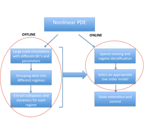
Figure 1: The offline-online approach to model based sensing and control of flows, incorporating various operating regimes. In this paper, we focus on DMD based offline extraction of subspaces and dynamics of various regimes from large scale simulation data, and online sparse sensing based regime selection and coarse reconstruction.

2 Dynamic Mode Decomposition

Dynamic mode decomposition is a recently developed data-driven dimensionality reduction and feature extraction method. It attempts to capture the underlying dynamic evolution of the data, such as that from simulation of a PDE. Consider a high-dimensional nonlinear system of the form

$$x(t+1)=f(x(t)),\quad x(0)=x_{0}\in\mathbb{R}^{n}$$ (1)

where our particular interest lies in models (1) arising from spatial discretization of a PDE via, e.g., finite elements, finite volumes, spectral elements. Below, we briefly present the DMD formulation following the work of in [53] and [17].

Let $s\in\mathbb{N}$ snapshots of the high-dimensional dynamical system (1) be arranged in two $n\times s$ data matrices

$$X_{0}:=[x(t_{0}),\ x(t_{1}),\ldots,x(t_{s-1})]\qquad\text{and}\qquad X_{1}:=[x(t_{1}),\ x(t_{2}),\ldots,x(t_{s})].$$

The dynamic evolution enters into the DMD formulation by assuming that a linear operator $A\in\mathbb{R}^{n\times n}$ maps $X_{0}$ to $X_{1}$, namely

$$X_{1}=AX_{0}.$$ (2)

Since the data is finite dimensional, the action of the operator can be represented as a matrix. The goal of DMD is to approximate the eigenvalues of $A$, using the data matrices only. The first step in DMD is to compute the singular value decomposition of $X_{0}=W\Sigma V^{T}$, so that we can approximate the snapshot set via

$$X_{0}\approx X_{0,r}=W_{r}\Sigma_{r}V_{r}^{T},$$ (3)

where $W_{r},V_{r}\in\mathbb{R}^{n\times r}$ contain the first $r$ columns of $W,V$, respectively, and $\Sigma_{r}$ is the leading $r\times r$ diagonal matrix of $\Sigma$. From the Schmidt-Eckart-Young-Mirsky theorem it follows that $||X_{0}-X_{0,r}||_{2}=\sigma_{r+1}$ (e.g., see [2, p. 37]), so if the singular values decay rapidly, the truncation error is small. A scaled version of the left singular vectors $W_{r}$ are the POD modes of the system. In DMD, however, we seek to extract dynamic information about $A$ by considering

$$X_{1}\approx AW_{r}\Sigma_{r}V_{r}^{T}.$$ (4)

Multiplying by $W_{r}^{T}$ from the left and by using the orthogonality of $V_{r}$, we obtain a reduced-order representation $A_{r}=W_{r}^{T}AW_{r}\in\mathbb{R}^{r\times r}$ of the system matrix $A$, namely

$$A_{r}:=W_{r}^{T}X_{1}V_{r}\Sigma_{r}^{-1},$$ (5)

which is (computationally) much cheaper to analyze than $A$. Next, compute the eigenvalue decomposition

$$A_{r}Y=Y\Lambda\quad\rightarrow W_{r}^{T}AW_{r}Y=Y\Lambda,$$ (6)

and by assuming $W_{r}W_{r}^{T}\approx I_{r}$ one can obtain an approximation for the decomposition

$$AW_{r}Y\approx W_{r}Y\Lambda,$$

and by defining $\Phi=W_{r}Y$, it follows that

$$A\Phi\approx\Phi\Lambda.$$ (7)

Here, $\Phi=[\phi_{1}\,\phi_{2}\,\dots\,\phi_{r}]$ contains the DMD modes $\phi_{m}$ as column vectors. Note, that the matrix $A_{r}$ is in general non-symmetric, and, therefore DMD modes will be complex. Nevertheless, the $r$-dimensional subspace of DMD modes $\Phi$ in the high-dimensional space $\mathbb{R}^{n}$ is the same as that spanned by $W_{r}$. Hence, the energy content kept in the DMD modes is the same as that for POD modes.

From a computational cost perspective, the dimensionality reduction due to the POD in (3) requires a reduced (economy) singular value decomposition of size $n\times s$, where $s\ll n$. The additional computation required in the DMD is the eigenvalue decomposition of size $s\times s$ in (6).

Remark 2.1.

The dynamic mode decomposition provides a non-orthogonal set of modes that attempt to capture the dynamic behavior of the model in a data-driven way. While non-orthogonal bases can burden computations, a breadth of work in DMD has shown that the added benefits of DMD can provide new insights into large-scale models with inherently low-dimensional dynamics [48, 53, 17, 59, 38, 12, 37, 63, 31, 46, 10, 58, 27]. We choose to work with DMD for multiple reasons:

1. DMD provides a data-driven alternative to other model reduction techniques and, as such, provides great flexibility. Galerkin projection-based model reduction techniques, such as POD, require building a low-dimensional system of ordinary differential equations for future state prediction. This in turn requires having access to, at least, the weak form of the partial differential equation model, and integration routines, which is intrusive. Additionally, problem specific correction terms, such as the shift-modes [40] or closure models [50] are often necessary to obtain accurate dynamic information for POD-Galerkin models.

2. The information encoded in the DMD modes provide a new viewpoint to the study of low-dimensional, coherent structures in flows, as evidenced in the pioneering work of [48, 53]. Every dynamic mode has an associated eigenvalue encoding its dynamic evolution. This yields additional information about spatial structures and their temporal evolution. For our purposes of short-term state prediction, temporal evolution extracted directly via DMD modes and eigenvales is justified via the following arguments. Under some conditions on the data [37, 59, 63], the DMD modes provide a linear basis for the evolution of observables, even if the underlying system is nonlinear. In particular, the action of the dynamical system on any finite set of observables is given by the Koopman operator $\mathcal{K}$, which is a infinite dimensional linear operator [38]. Assuming that the discrete time evolution of the PDE is given by $x(t+1)=f(x(t))$, the Koopman operator acts on any scalar observable $g(x)$ as

   $$\mathcal{K}g(x)=g(f(x)).$$

   A vector valued observable, such as $h\in\mathbb{R}^{n}$ can be expanded in terms of the (scalar) Koopman eigenfunctions of $\mathcal{K}$, $\{\theta_{j}\}_{j=0}^{\infty}$, and vector valued Koopman modes, $\{\phi_{j}\}_{j=0}^{\infty}$ as

   $$h(x)=\sum\limits_{j=0}^{\infty}\theta_{j}(x)\phi_{j}.$$

   Applying the Koopman operator on $h$, we obtain

   $$h(f(x))=\sum\limits_{j=0}^{\infty}\lambda_{j}\theta_{j}(x)\phi_{j}.$$

   Given a data set, the unknown scalars $\theta_{j}(x)$ can be computed, for example, by projecting on initial conditions, or using some other way of reducing the overall error in the approximation [31]. In particular, using $\beta_{j}=\theta_{j}(x)$ to simplify notation, the above expansion takes the form

   $$\begin{bmatrix}x(t_{1})&x(t_{2})&\ldots&x(t_{s})\end{bmatrix}\approx\begin{bmatrix}\phi_{1}&\phi_{2}&\dots&\phi_{r}\end{bmatrix}\begin{bmatrix}\beta_{1}&&&\\ &\beta_{2}&&\\ &&\ddots&\\ &&&\beta_{r}\end{bmatrix}\begin{bmatrix}1&\lambda_{1}&\ldots&\lambda_{1}^{s-1}\\ 1&\lambda_{2}&\ldots&\lambda_{2}^{s-1}\\ \vdots&\vdots&\ddots&\vdots\\ 1&\lambda_{r}&\ldots&\lambda_{r}^{s-1}\\ \end{bmatrix},$$

   where the observable is now a snapshot $x(t_{i})$ of the finite-dimensional system (1). In fact, the DMD and the related Koopman mode decomposition have been used to explain the origin and success of various modifications to POD-Galerkin system, such the shift-modes [40].

3. The connection of DMD to many established techniques, such as the Floquét decomposition of linear systems [53], the Fourier decomposition, and the eigensystem realization algorithm [59]. Those connections raise further interesting research questions.

We note that DMD has several limitations, which are well-documented in the recent literature. While the original DMD algorithm is successful in resolving the dynamics on system attractors (and in some small neighborhoods of these attractors [4]), several questions remain on its validity for accurately modeling off-attractor dynamics. However, recent efforts have been directed at accurate extraction of DMD modes (and Koopman modes) for general off-attractor dynamics [63, 39], and rigorously proving their accuracy in the basin of attraction of these attractors [33]. Hence, as these methods become mature, we expect that our algorithm can be useful for off-attractor dynamics too.

3 Flow in Two-dimensional Differentially Heated Cavity

To demonstrate our approach, we consider the two dimensional upright differentially heated cavity problem. This is one of the fundamental flow configurations for heat transfer and fluid mechanics studies, and has numerous applications including reactor insulation, cooling of radioactive waste containers, ventilation of rooms and solar energy collection, among others [44]. Figure 2 provides an illustrative schematic of the problem along with the corresponding boundary conditions.

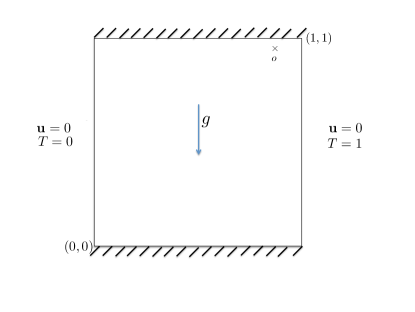
Figure 2: Schematic of the differentially heated cavity problem. The top and bottom walls are insulated and the left and right walls are maintained at a constant distinct temperature. The direction of the gravity is downward. We use two monitoring points marked by ‘o’ at $(x,y)=(0.85,0.88)$, and the marker ‘x’ represents location $(x,y)=(0.87,0.93)$.

The domain is a two dimensional enclosure with insulated top and bottom walls, and the left and right walls serve as hot and cold isothermal sources. We assume the aspect ratio of the cavity is unity; nonetheless, it should be noted that the variation in aspect ratio alters the features of the flow non-trivially. The flow is driven due to buoyancy forces; the temperature difference between the walls results in a gravitational force exerted on the volume of the fluid that initiates the flow. The heated fluid rises along the hot wall, while cooled fluid is falling along the cold wall. When the heated fluid reaches the top wall, it spreads out to the other side in a form of the gravity current. In our simulations, the Prandtl number $Pr$ is 0.71, which is a typical value for air. The temperature difference and other fluid properties are chosen such that the Rayleigh number, defined as $Ra=\frac{\rho^{2}g\tau\Delta TH^{3}}{\mu^{2}}Pr$, varies between $10^{1}<Ra<10^{9}$.

3.1 Governing equations and numerical scheme

The Boussinesq equations model the viscous, convective fluid motion associated with buoyancy forces, therefore serving as the model for natural convection. The Boussinesq equations for an incompressible fluid are given by

$$\nabla\cdot\mathbf{u} =0$$ (8)

$$\mathbf{u}_{t} =\mu\Delta\mathbf{u}-(\mathbf{u}\cdot\nabla)\mathbf{u}-\nabla p+g(\rho-\rho_{0})$$ (9)

$$T_{t} =\kappa\Delta T-\mathbf{u}\cdot\nabla T,$$ (10)

where $T(\cdot,\cdot)$ is the temperature field and $\mathbf{u}(\cdot,\cdot)=[u_{x},u_{y}]^{T}$ is the fluid velocity. If the Boussinesq approximation is applied, the last term in the momentum equation (9) becomes

$$g(\rho-\rho_{0})=\rho_{0}g\tau(T-T_{0}),$$ (11)

where $\tau$ is the coefficient of thermal expansion and $T_{0}$ is the reference temperature at which $\mu$, $Pr$ and $\rho_{0}$ are defined.

To numerically solve the equation and obtain simulation data, we use the open source spectral-element solver NEK5000 [42, 45, 30]. Owing to their high accuracy and general usage, spectral methods are particularly suited to the study of transition to turbulence in near-to-wall flows, including natural convection within differentially heated cavities.

3.2 DNS Results and Discussion

This problem has been extensively studied and accurate solutions are available in the literature for comparison; see, e.g., [29, 36, 34]. In Figure 3, we plot the Nusselt numbers computed using our simulation data, along with the corresponding values in [36]. Our results are in close agreement with the data of [36]. Since any inaccuracies in resolving near-wall effects will manifest themselves in heat-flux calculations, close agreement in Nusselt numbers with previously reported data in the literature provides evidence of validity of our numerical solver.

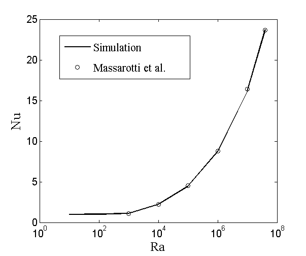
Figure 3: Nusselt numbers from our simulations compared with data from [36].

A circulatory flow is set up in a vertical layer that is bounded by isothermal surfaces thermally insulated at the ends, having different temperatures. The flow ascends against the hot surface and descends at the cold surface. For smaller Rayleigh number, $Ra<10^{8}$, the flow field reaches a steady state, that is $\partial\mathbf{u}/\partial t=\partial T/\partial t=0$. It is well-established that at steady state, the temperature away from the boundary layers increases linearly over a large part of the height of the layer [44]. Hence, for those values of Rayleigh numbers, the steady state is stable near the corners of the cavity as well within the boundary layer close to the walls.

As the Rayleigh number increases, the flow loses stability. When $Ra\geq Ra_{c}$, where $Ra_{c}$ is critical Rayleigh number, first the flow in the corners and then the flow in the thermal boundary layer become increasingly unstable. For large Rayleigh numbers, say, $Ra>10^{9}$ the flow becomes turbulent. When a statistical steady state is reached, the space between the vertical boundary layers is filled by a virtually immobile stably stratified fluid exhibiting low-frequency, low-velocity oscillations.

To better understand the behavior, we examine time series data from local velocity and temperature measurements at the spatial location $(x,y)=(0.85,0.88)$. The temperature at this location reaches a steady-state asymptotic value after a finite time. By increasing the Rayleigh number, however, the nature of the flow undergoes a transition. Consistent with [34], we observe that the onset of unsteadiness takes place at a critical $Ra_{c}=1.82\times 10^{8}$ and that the first instability mode breaks the usual centro-symmetry of the solution. Figure 4(a) illustrates the streamlines at this Rayleigh number. The onset of unsteadiness in velocity indicates oscillations in the temperature field as well. Hence, the time series of the temperature at the monitoring point shows an asymptotic finite-amplitude periodic state. The period of such oscillations is measured from DNS data by using the power spectral density (PSD) as shown in Figure 4(b).

This transition to periodic behavior has been studied in [34]. By numerically computing the spectrum of the linearized Boussinesq equations operator for Rayleigh numbers below and above the transition value, it is shown that this transition is a supercritical Hopf bifurcation. Physically, this instability takes place at the base of the detached flow region along the horizontal walls and is referred to as the ‘primary instability mechanism’. The frequency associated with the primary instability mechanism can be seen in Figures 4(b) and 5(b) to be around $\omega=0.045Hz$, close to the value reported in [34].

With respect to the fluctuating temperature, for $Ra\geq Ra_{c}$, we observe that away from the corners of the cavity, the contour lines are inclined at an angle of approximately 20 degrees with respect to the horizontal, and they propagate in time orthogonally to their direction. These lines, shown in Figure 5(a) for $Ra=2\times 10^{8}$, correspond to the wavefronts of internal waves, which are shed from the region where the instability mechanism takes place.

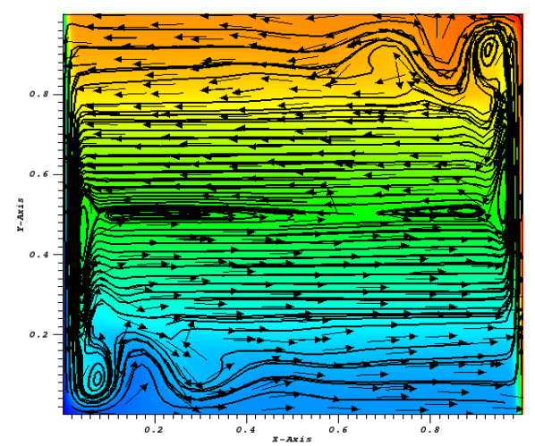
(a) Streamlines and velocity vectors superposed by temperature psuedocolor (from red to right, the temperature varies from hot to cold).

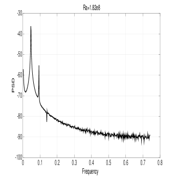
(b) Power spectrum density of temperature time series at location $(x,y)=(0.85,0.88)$.

Figure 4: Flow solution at $Ra=1.82\times 10^{8}$.

By increasing the Rayleigh number such waves propagate into the domain as shown in Figure 6(a) for $Ra=4\times 10^{8}$. In addition, we examine the location $(x,y)=(0.87,0.93)$, closer to the wall than the one chosen above. At this Rayleigh number, the existence of a ‘secondary instability mechanism’ has been reported [34] at a frequency close to $\omega=0.48Hz$. In Figure 6(b), we can see that this instability is also observed in our simulation data.

The conjecture in [34] is that the secondary instability mechanism is a local phenomenon that originates from the boundary layer at the top wall. Hence, the monitoring point away from the wall does not capture the resulting localized oscillations. For even higher Rayleigh numbers, the solutions depend strongly on the initial condition, and multiplicity of the solutions is also observed. For these higher Rayleigh numbers, the oscillations in temperature do not show a periodic behavior and the flow becomes chaotic.

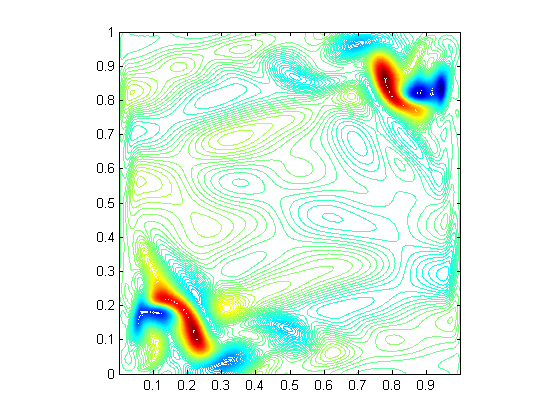
(a) Instantaneous fluctuating temperature fields.

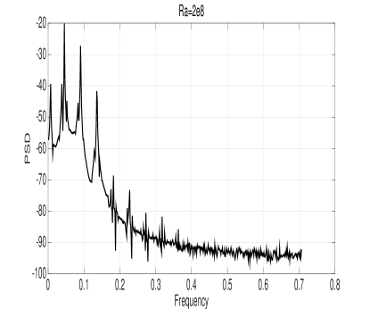
(b) Power spectrum density of temperature at location $(x,y)=(0.85,0.88)$.

Figure 5: Flow solution at $Ra=2\times 10^{8}$.

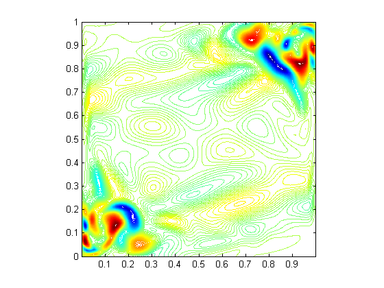
(a) Instantaneous fluctuating temperature fields.

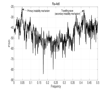
(b) Power spectrum density of temperature at location $(x,y)=(0.87,0.93)$.

Figure 6: Flow solution at $Ra=4\times 10^{8}$.

For a variety of parameter settings we compute the DMD from the simulation data. For simplicity we compute the same number of modes for all different parameters. In particular we find that $r=20$ modes capture more than $99\%$ of the system energy in all cases.

We show the dynamic separation that DMD provides for the spatial modes in Figure 7(a). We plot the energy content of the DMD modes at different frequencies obtained from the corresponding DMD eigenvalues. The dominant DMD mode, other than the ‘base’ flow at zero frequency, has frequency $\omega\approx 0.045Hz$, close to frequency associated with the primary instability discussed earlier. The absolute value of this DMD mode is also plotted over the domain in Figure 7, along with the next dominant DMD mode. Figure 8 shows a DMD mode at frequency $\omega\approx 0.02Hz$ and another DMD mode at frequency close to the secondary instability frequency $\omega\approx 0.4Hz$. The mode corresponding to the primary instability was not found among the dominant DMD modes at this Rayleigh number. This implies that the secondary instability mechanism is not only localized in space, but also has minimal signature in the data in $l_{2}$ sense. For even higher Rayleigh numbers, DMD modes at several different frequencies have large and comparable magnitudes, which could be interpreted as a signature of chaotic behavior.

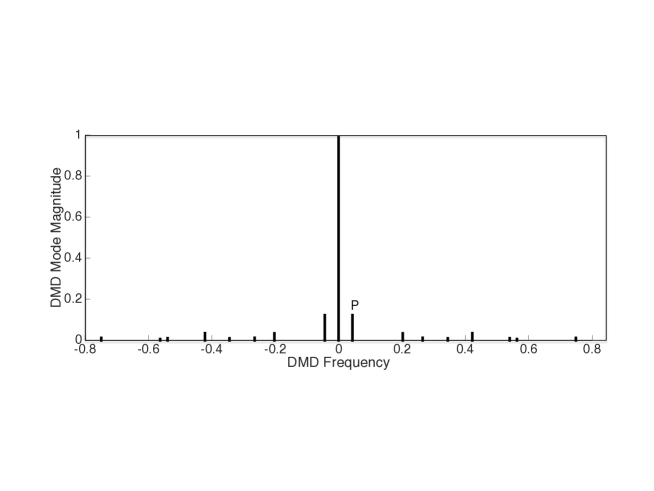
(a) The spectrum of DMD eigenvalues, with corresponding frequencies and DMD mode magnitude. The bar marked ’P’ refers to the primary instability frequency discussed in Section 3.

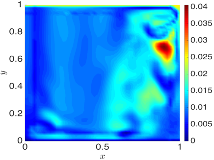
(b) DMD mode corresponding to frequency $\omega\approx 0.04Hz$ marked ’P’ in plot (a).

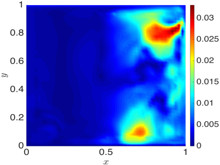
(c) DMD mode corresponding to frequency $\omega\approx 0.2Hz$.

Figure 7: DMD modes and spectrum for $Ra=2\times 10^{8}$.

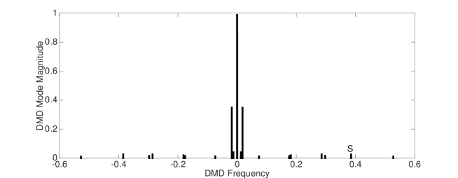
(a) The spectrum of DMD eigenvalues, with corresponding frequencies and DMD mode magnitude. The bar marked ’S’ refers to the secondary instability frequency discussed in Section 3.

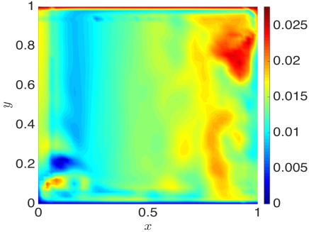
(b) DMD mode corresponding to frequency $\omega\approx 0.02Hz$.

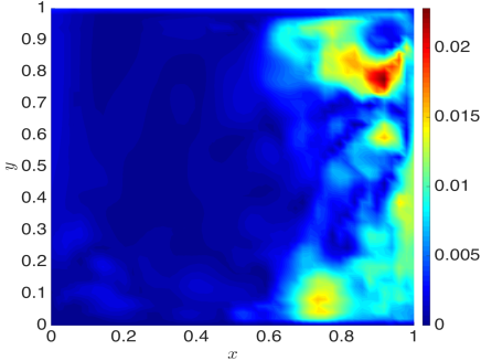
(c) DMD mode with frequency marked ’S’ $\omega\approx 0.4Hz$.

Figure 8: DMD modes and spectrum for $Ra=4\times 10^{8}$.

4 Robust Classification by Augmenting DMD Basis

We propose a regime classification approach based on the premise that if a system operates in a particular regime, then snapshots of the system, and, therefore of the measurements, lie in a low-dimensional subspace particular to the regime. Thus, our regime detection approach uses offline computation to build a library of subspaces, as introduced in Section 4.1. This general setting allows for any low-dimensional subspace, or reduced-order model technique to be used for the library generation technique. In Section 4.2 we introduce the classification problem for a single snapshot in time. We then derive our new method in Section 4.3, where we augment the DMD basis by using dynamical information. This particular method heavily relies on the dynamic properties extracted from the DMD. Section 4.4 incorporates the augmented DMD basis into the classification of time-sequential measurements of the same dynamic regime, providing a more robust sensing mechanism. In Sections 4.5 and 4.6 we then provide a classification analysis, and introduce metrics to assess the quality of the classification.

4.1 Library generation

First, we compute a library of dynamic regimes by using subspaces that are generated from a variety of configurations and boundary conditions, each leading to a different regime. Thus, let $\mathcal{Q}=\{q_{1},q_{2},\ldots,q_{d}\}$ denote the set of $d$ different parameters used to generate the library. For each parameter $q_{i}\in\mathcal{Q}$, we obtain data from solving the high dimensional model (1). The data are stored in $X_{i}:=X(q_{i})\in\mathbb{R}^{n\times s}$, where each column of $X(q_{i})$ is a snapshot of the solution of (1) associated with parameter $q_{i}$. Next, we compute $r_{i}$ basis functions for every regime, $i=1,\ldots,d$, and store them in $\Phi(q_{i}):=\Phi_{i}$, a basis for the low-dimensional subspace for the dynamic regime. The set of all such bases $\Phi_{i}\in\mathbb{R}^{n\times r_{i}}$ defines a library

$$\mathcal{L}:=\{\Phi_{1},\Phi_{2},\ldots,\Phi_{d}\}.$$

4.2 Classification for single time snapshots

We use a simple classification algorithm to identify the subspace (and hence the regime) in the library which is most aligned with the current system measurements.

Our measurements are obtained using a linear measurement matrix $C\in\mathbb{R}^{p\times n}$. The measurement matrix $C$ can represent a large number of possible measurement systems. For example, point measurements of the $j$th component of $x$ are obtained using rows of $C$ that are zero everywhere except the $j$th component, where they take the value of one. Thus, a system using only distinct single point measurements satisfies

$$C_{i,j}:=\{0,1\},\qquad\sum_{j=1}^{n}C_{i,j}=1,\ i=1,\ldots,p,\qquad\sum_{i=1}^{p}C_{i,j}=1,\ j=1,\ldots,n.$$

Alternatively, tomographic measurements, which integrate along one or more particular directions, can be represented by placing ones on all the locations along the direction which is integrated. Of course, $C$ may also be the identity matrix or another complete basis for the space. In that case, $p=n$ and the matrix preserves the full state information from the system. In other words, our regime identification approach can be used on the full state, if available, instead of sparse measurements. Since this is not typical in practical applications, the subsequent exposition assumes that a sensing system is used, with $p\ll n$.

In practice, the measurements $y(t)\in\mathbb{R}^{p}$ are often noisy, so that

$$y(t)=Cx(t)+\xi,$$

where $\xi$ is a noise process, often assumed to be of zero mean and unit variance, i.e., white noise. Assuming that a low-order representation of the $k$th regime represents $x(t)$ in $\Phi_{k}$, the measurements should lie in the subspace spanned by the $p\times r_{k}$ matrix

$$\Theta_{k}=C\Phi_{k}.$$

Correspondingly, a regime library for the observations is given by

$$\mathcal{L}_{obs}=\{\Theta_{1},\ \Theta_{2},\ldots,\Theta_{d}\}.$$ (12)

Given the measurements, we identify the regime $k^{\star}$ as the subspace in the library $\mathcal{L}_{obs}$ closest to the measurements in an $\ell_{2}$ sense:

$$k^{\star}=\arg\min_{k=1,\ldots,d}\left\{\min_{\beta_{k}}\|y(t)-\Theta_{k}\beta_{k}\|_{2}\right\},$$ (13)

where $\beta_{k}$ denotes the unknown coefficients in the subspace basis $\Theta_{k}$. Consequently, $\beta^{\star}_{k}$ is the least square solution to the system

$$\beta^{\star}_{k}=\Theta_{k}^{\dagger}y(t),$$ (14)

where $(\cdot)^{\dagger}$ denotes the Moore-Penrose pseudoinverse. The operator $P_{k}=\Theta_{k}\Theta_{k}^{\dagger}$ is a projection operator onto the span of $\Theta_{k}$ and the classification algorithm can be expressed as

$$k^{\star}=\arg\min_{k=1,\ldots,d}\|y(t)-P_{k}y(t)\|_{2}=\arg\max_{k=1,\ldots,d}\|P_{k}y(t)\|_{2}.$$ (15)

Classification, in other words, projects the measured data $y(t)$ to the span of each basis set $\Theta_{k}$ and determines which projection is closest to the acquired data. Because of the orthogonality of the projection error, this is equivalent to maximizing the norm of the projection. The underlying classification assumption, which we formalize in the next section, is that the regimes span sufficiently dissimilar subspaces and that measurements originating from one regime have smaller projections onto the subspaces describing the other regimes. If the regime $k$ is identified correctly, then

$$x^{\star}(t)=\Phi_{k}\beta^{\star}_{k}=\Phi_{k}\Theta_{k}^{\dagger}y(t),\qquad\Phi_{k}\in\mathcal{L},\ \ \Theta_{k}\in\mathcal{L}_{obs},$$

approximates the system state $x(t)\in\mathbb{R}^{n}$ from the measurements $y(t)\in\mathbb{R}^{p}$. Using $x^{\star}(t)$ as an initial state estimate, estimation of the full state vector in future can then be obtained by using the associated local reduced order model (DMD -based or Galerkin approximation-based), and an associated state-space observer, e.g., Luenberger observer for the DMD-based local model.

For the classification given by equation (15) to be successful, the number of measurements, i.e., the dimensionality of $y(t)$, should be greater than the dimensionality of the subspace of each regime, i.e., $p>\max_{k}[\mathrm{rank}\ \Theta_{k}]$. Otherwise the projection error to that regime is zero. However, the number of measurements needed is significantly less than the $total$ dimension of subspaces of all regimes, $r=\sum_{k}\mathrm{rank}\ \Theta_{k}$ (or equivalently, $\sum_{k}r_{k}$). In other words, we have the following ordering on the dimension of various quantities, $p\ll r\ll n$, similar to the ordering in [11]. This ordering is often present in Compressed Sensing literature [16]. This may still imply a large number of sensors if only a single time snapshot is used for classification. This issue is significantly alleviated if we exploit the dynamic information given by the DMD, and use the time augmentation approach we describe in the next section.

Remark 4.1.

Note that the measurement matrix $C$ might have a nullspace that eliminates some of the basis elements in $\Phi_{i},i=1,\ldots,d$. Subspace-based identification cannot, therefore, exploit any information along these basis elements. This can be avoided, for example, using matrices typical in compressive sensing applications. These include matrices with entries drawn from i.i.d. Gaussian or Bernoulli distributions, which are unlikely to have any of the basis elements in their nullspace—a property known as incoherence (e.g., see [16]). However, such matrices are difficult to realize in physical systems. Point and tomographic sensors are more typical in such systems. Thus, sensor placement, an issue we briefly discuss later but do not address in this paper, can significantly affect system performance.

4.3 Augmented DMD – Incorporating dynamics into basis

We propose a method to incorporate the dynamic information given by the DMD of the data into the basis generation. Consider a state vector $x(t)$ , sampled from the underlying dynamical system at time $t$. To keep notation minimal, we first consider a single dynamic regime and drop the subscripts which would indicate regime membership. To begin with, let the state be expressed in the sparse DMD basis as

$$x(t)=\Phi\beta(t),$$

where $\beta(t)\in\mathbb{C}^{r}$ is again the unknown vector of coefficients. Recall, that by equation (7), the DMD basis approximates the eigenvectors of the advance operator $A$. Consequently, $A\Phi=\Phi\Lambda$, where $\Lambda$ denotes the diagonal matrix of the first $r$ eigenvalues of $A$. From the one-step-advance property of the linear operator $A$, we have

$$x(t+1)=Ax(t)=A\Phi\beta(t)=\Phi\Lambda\beta(t),$$

and iteratively

$$x(t+j)=A^{j}x(t)=\Phi\Lambda^{j}\beta(t).$$

Therefore, subsequent snapshots can be expressed via the same $r$-dimensional vector $\beta(t)$ (and hence the same regime). Therefore, we have more data to make a confident classification decision. In particular, the above information can be written in batch-form as

$$\begin{bmatrix}x(t)\\ x(t+1)\\ \vdots\\ x(t+j)\end{bmatrix}=\begin{bmatrix}\Phi\beta(t)\\ \Phi\Lambda\beta(t)\\ ...\\ \Phi\Lambda^{j}\beta(t)\end{bmatrix}=\begin{bmatrix}\phi_{1}&\phi_{2}&\ldots&\phi_{r}\\ \lambda_{1}\phi_{1}&\lambda_{2}\phi_{2}&\ldots&\lambda_{r}\phi_{r}\\ \vdots&\vdots&&\vdots\\ \lambda_{1}^{j}\phi_{1}&\lambda_{2}^{j}\phi_{2}&\ldots&\lambda_{r}^{j}\phi_{r}\\ \end{bmatrix}\cdot\beta(t).$$

Next, we define the augmented DMD basis vector as

$$\widehat{\phi}_{i,j}:=\begin{bmatrix}\phi_{i}\\ \lambda_{i}\phi_{i}\\ \vdots\\ \lambda_{i}^{j}\phi_{i}\end{bmatrix}\quad\in\mathbb{C}^{(j+1)n},\quad\text{with}\quad\widehat{\phi}_{i,0}:=\phi_{i},$$

so that the previous equation can be rewritten as

$${x}(t:t+j)=\begin{bmatrix}x(t)\\ x(t+1)\\ \vdots\\ x(t+j)\end{bmatrix}=\begin{bmatrix}\widehat{\phi}_{1,k}\ \widehat{\phi}_{2,k}\ \ldots\ \widehat{\phi}_{r,k}\end{bmatrix}\cdot\beta(t)=\widehat{\Phi}\beta(t).$$ (16)

When considering the outputs of the dynamical system, $y(t)=Cx(t)$, the recursion remains unchanged. Thus, using $C\in\mathbb{R}^{p\times r}$ to denote, as above, the sensing matrix, we define

$$\mathcal{C}=\begin{bmatrix}C&0&\ldots&0\\ 0&C&\ldots&0\\ \vdots&\vdots&\vdots&\vdots\\ 0&0&\ldots&C\end{bmatrix}_{p(j+1)\times r(j+1)}.$$ (17)

and the sensed augmented DMD basis as

$$\widehat{\Theta}_{k}:=\mathcal{C}\widehat{\Phi}_{k}.$$ (18)

We can now define the library of augmented DMD modes.

Definition 4.2.

Let the DMD modes be $\Phi_{i}=\Phi(q_{i})\in\mathbb{C}^{n\times r_{i}}$, and let the diagonal matrix of $r_{i}$ eigenvalues $\Lambda_{i}=\Lambda_{r_{i}}(q_{i})$ of each dynamic regime $i$, where $i=1,\ldots,d$, be given. The augmented DMD library is defined as

$$\widehat{\mathcal{L}}:=\left\{\begin{matrix}\begin{bmatrix}\Phi_{1}\\ \Phi_{1}\Lambda_{1}\\ \cdots\\ \Phi_{1}\Lambda_{1}^{j}\end{bmatrix},\begin{bmatrix}\Phi_{2}\\ \Phi_{2}\Lambda_{2}\\ \cdots\\ \Phi_{2}\Lambda_{2}^{j}\end{bmatrix},\ldots,\begin{bmatrix}\Phi_{d}\\ \Phi_{d}\Lambda_{d}\\ \cdots\\ \Phi_{d}\Lambda_{d}^{j}\end{bmatrix}\end{matrix}\right\}=\left\{\widehat{\Phi}_{1},\widehat{\Phi}_{2},\ldots,\widehat{\Phi}_{d}\right\}.$$ (19)

Similarly, using $\mathcal{C}$ from (17), define the observation library as

$$\widehat{\mathcal{L}}_{obs}:=\left\{\mathcal{C}\widehat{\Phi}_{1},\mathcal{C}\widehat{\Phi}_{2},\ldots,\mathcal{C}\widehat{\Phi}_{d}\right\}=\left\{\widehat{\Theta}_{1},\widehat{\Theta}_{2},\ldots,\widehat{\Theta}_{d}\right\}.$$

4.4 Classification with time-augmented DMD basis

To increase robustness of the classification and measuring process, we extend the classification problem from Section 4.2 to using multiple time measurements

$$y(t:t+j)=[y(t)^{T}\ y(t+1)^{T}\ y(t+j)^{T}]^{T}.$$

Multiplying (16) by $\mathcal{C}$ from the left (i.e., using only sensed information), the classification problem with the augmented DMD basis can then be recast as finding

$$k^{\star}=\arg\min_{k=1,\ldots,d}\left\{\min_{\beta_{k}(t)}\|{y}(t:t+j)-\widehat{\Theta}_{k}\beta_{k}(t)\|_{2}\right\}.$$

Similarly to the least-squares solution from data at a single time, see  (14), the least-squares estimate for the coefficients is computed via the pseudoinverse of $\widehat{\Theta}_{i}$, i.e.,

$$\beta^{\star}_{k}(t)=\widehat{\Theta}_{k}^{\dagger}y(t:t+j).$$ (20)

In order to cast the classification as a maximization of the projection energy, as in (15), the corresponding projection operator for $y_{k}(t:t+j)$ is $\widehat{P}_{k}=\widehat{\Theta}_{k}\widehat{\Theta}_{k}^{\dagger}$. Hence, the solution is given by projection,

$$k^{\star}=\arg\max_{k=1,\ldots,d}\|\widehat{P}_{k}{y}(t:t+j)\|_{2}.$$ (21)

Note that $y(t:t+j)\in\mathbb{R}^{p(j+1)}$ is the available data, and $\beta_{i}(t)\in\mathbb{C}^{r_{i}}$. Therefore, we still have to find $r_{i}$ coefficients, but this time we can use data of length $p(j+1)$, where $j$ is the length of the data window to be specified. In the numerical results reported in Section 5, we will see that $j\leq 10$ is often sufficient to robustly classify a signal to the correct subspace.

In other words, the time augmentation exploits the dynamic information provided by DMD to increase the amount of data over time, while keeping the number of spatial sensors the same. This comes at the expense of a small delay waiting to collect $j$ time snapshots. Moreover, an improvement is also evident in several library measures that are used in the compressed sensing community, particularly the alignment and coherence metrics which we define in the following sections.

Remark 4.3.

Single time-snapshot classification is, of course, possible using POD-based reduced models and libraries. However, as evident from our development, exploiting the time-evolution dynamics requires the use of DMD modes and the DMD-derived eigenvalues. As we see in the numerical results below, this significantly increases robustness of the classification method, particularly in the presence of sensor noise. Moreover, it improves classification accuracy in general.

4.5 Classification Performance Analysis

In this section we develop bounds and metrics that can be used to guarantee correct classification under the worst-case conditions. As we observe later in Section 5, these metrics can be conservative in practice; however, classification performance is better than what the bounds suggest. Still, they show the classification performance trends and provide clear intuition on the role of the subspaces and their similarity in classification. The metrics we discuss here and in the next section can be used both with a single snapshot, using the tools described in Section 4.2, and with multiple snapshots in the context of augmented DMD described in Section 4.4.

Assume that the system is operating under regime $k$ (we will use superscripts in this section to denote dependence on the regime) and that noiseless measurements

$$y_{k}(t)=Cx_{k}(t),$$ (22)

are obtained at a single time instance, or over an extended time interval $(t:t+j)$. To simplify notation, and encompass both cases, for the remainder of this section we use $y_{k}$ to denote the measurements, either from a single or multiple snapshots in time. We also omit $\widehat{\cdot}$ from the definitions of projections. The classification algorithm identifies the best matching projection of the data, $P_{k^{\star}}y_{k}$, and determines the estimated regime as $k^{\star}$. Our goal is to determine metrics and guarantees under which classification is successful, i.e., $k^{\star}=k$. To that end we define the subspace $\mathcal{W}_{k}$ for each $k$, spanned by the basis functions $\Theta_{k}$. Given that the measurements originate from regime $k$, most of their energy lies in $\mathcal{W}_{k}$. To formalize this statement, we first decompose the measurements to a direct sum of an in-space approximation component $\widetilde{y}_{k}$ and an approximation error component $\widetilde{y}_{k}^{\perp}$, which is orthogonal to the space

$$y_{k}=\widetilde{y}_{k}+\widetilde{y}_{k}^{\perp},\qquad\widetilde{y}_{k}\in\mathcal{W}_{k},\qquad\widetilde{y}_{k}^{\perp}\perp\mathcal{W}_{k}.$$ (23)

The latter component is due to the approximation performed as part of the dimensionality reduction. This approximation is accurate if $\|\widetilde{y}_{k}(t)^{\perp}\|_{2}\leq\epsilon\|\widetilde{y}_{k}(t)\|_{2}$ for some small $\epsilon$ which bounds the approximation error.

Furthermore, we define a metric for subspace alignment, which measures subspace similarity by determining the vectors in one subspace that are most similar to their projection in the other subspace:

$$\eta_{jk}:=\|P_{j}P_{k}\|_{2}=\max_{~{}\forall y}\frac{||P_{j}P_{k}y||_{2}}{||y||_{2}},\quad j,k\in\{1,\ldots,d\}.$$ (24)

Using this metric, which is always less than 1, we can show the following proposition.

Proposition 4.4.

Let $d$ subspaces $\mathcal{W}_{j},\ j=1,\ldots,d$ be given, and let the signal $\widetilde{y}_{k}\in\mathcal{W}_{k}$ for some $k\in 1,\ldots,d$ according to (23), and $t>0$. Moreover, assume that $\|\widetilde{y}_{k}^{\perp}\|_{2}\leq\epsilon\|\widetilde{y}_{k}\|_{2}$, with $\eta_{jk}$ defined in (24). Then, if

$$\eta=\max_{j\neq k}\eta_{jk}<1-\epsilon$$ (25)

the classification in (15) is successful.

Before proving the proposition, we provide a brief discussion on the relevant quantities and a small example application. In particular, given a set of $d$ subspaces, the $\eta_{jk}$ are quantities easily computable using simple linear algebra in low dimensions. Furthermore, the worst-case alignment $\eta$ can be used to formulate the guarantee: given a set of subspaces, we should expect to always classify signals correctly if $\eta$ satisfies (25). This in turn gives a priori guidance on whether a dictionary is suitable for classification, or if two regimes have similar behavior with respect to their corresponding subspaces. In the following example, we provide some intuition on the robustness of the alignment measure and our bounds.

Example 4.5.

Let us consider two subspaces $\mathcal{W}_{j}$ and $\mathcal{W}_{k}$, and assume all signals from regime $k$ contain at least $90\%$ of their energy in the subspace $\mathcal{W}_{k}$, i.e., $\epsilon=.1$. Consequently, if $\eta_{jk}<.9$, we guarantee correct classification of the signal $y_{k}$ to the subspace $\mathcal{W}_{k}$ for all $t>0$.

Proof.

To demonstrate the proposition, we start with the decompositon $y_{k}=\widetilde{y}_{k}+\widetilde{y}_{k}^{\perp},~{}\widetilde{y}_{k}\in\mathcal{W}_{k},~{}\widetilde{y}_{k}^{\perp}\perp\mathcal{W}_{k},$ as above. Since $\widetilde{y}_{k}^{\perp}\perp\mathcal{W}_{k}$, the projection onto the correct subspace is equal to

$$P_{k}y_{k}=\widetilde{y}_{k},$$

i.e., has norm equal to

$$\|P_{k}y_{k}\|_{2}=\|\widetilde{y}_{k}\|_{2}.$$ (26)

The projection onto the other subspaces is equal to

$$P_{j}y_{k}=P_{j}\widetilde{y}_{k}+P_{j}\widetilde{y}_{k}^{\perp}=P_{j}P_{k}\widetilde{y}_{k}+P_{j}\widetilde{y}_{k}^{\perp},$$

which, using the triangle inequality and the trivial bound $\|P_{j}\widetilde{y}_{k}^{\perp}\|_{2}\leq\|\widetilde{y}_{k}^{\perp}\|_{2}$ for any projection $P_{j}$, has norm bounded by

$$\|P_{j}y_{k}\|_{2}\leq\|P_{j}P_{k}\widetilde{y}_{k}\|_{2}+\|P_{j}\widetilde{y}_{k}^{\perp}\|_{2}\leq\|P_{j}P_{k}\|_{2}\|\widetilde{y}_{k}\|_{2}+\|\widetilde{y}_{k}^{\perp}\|_{2}\leq\eta\|\widetilde{y}_{k}\|_{2}+\|\widetilde{y}_{k}^{\perp}\|_{2}.$$ (27)

The classification will be accurate if the projection onto the subspace corresponding to regime $k$ preserves more energy than all other projections, i.e., if

$$\|P_{j}y_{k}\|_{2}\leq\|P_{k}y_{k}||_{2},\quad\mbox{for~{}all~{}}j\in\{1,\ldots,d\},j\neq k.$$

Rewriting equation (25) as

$$\eta\|\widetilde{y}_{k}\|_{2}+\epsilon\|\widetilde{y}_{k}\|_{2}<\|\widetilde{y}_{k}\|_{2}=\|P_{k}y_{k}\|_{2},$$ (28)

where at most a portion $\epsilon$ of the signal lies out of the correct subspace $\|\widetilde{y}_{k}^{\perp}\|_{2}\leq\epsilon\|\widetilde{y}_{k}\|_{2}$, i.e.,

$$\eta\|\widetilde{y}_{k}\|_{2}+\|\widetilde{y}_{k}^{\perp}\|_{2}\leq\eta\|\widetilde{y}_{k}\|_{2}+\epsilon\|\widetilde{y}_{k}\|_{2}<\|\widetilde{y}_{k}\|_{2}=\|P_{k}y_{k}\|_{2}$$ (29)

Using (27) it follows that for all $j\neq k$

$$\|P_{j}y_{k}\|_{2}\leq\eta\|\widetilde{y}_{k}\|_{2}+\|\widetilde{y}_{k}^{\perp}\|_{2}\leq\eta\|\widetilde{y}_{k}\|_{2}+\epsilon\|\widetilde{y}_{k}\|_{2}<\|\widetilde{y}_{k}\|_{2}=\|P_{k}y_{k}\|_{2}.$$ (30)

Thus, the length of the projection to other subspaces is always lower than the length of the projection to the correct subspace and the regime is correctly classified. ∎

4.6 Block Sparse Recovery and Classification

In addition to the subspace alignment measure $\eta$ introduced in Section 4.5, the measures of block-coherence between different regimes, and sub-coherence within each regime, can help to understand the classification performance and requirements on the library (12). These measures are drawn from the block-sparse recovery and the compressive sensing literature (e.g., see [19, 8] and references therein).

Block sparsity models split a vector into blocks of coefficients and impose that only some of the blocks contain non-zero coefficients.

Definition 4.6.

Let $r=\sum_{i=1}^{d}r_{i}$ and $\beta_{i}\in\mathbb{C}^{r_{i}}$. The vector $\beta=[\beta_{1}^{\ast}\ \beta_{2}^{\ast}\ \ldots\ \beta_{d}^{\ast}]^{\ast}\in\mathbb{C}^{r}$ is called block $s$-sparse, if $s$ of its blocks $\beta(q_{i})$ are nonzero.

Using the above definition, we have that $y(t)=[\Theta_{1},\Theta_{2},\ldots,\Theta_{d}]\ \beta$, with only $s$ blocks of coefficients in $\beta$ being nonzero, namely the blocks corresponding to the active regimes. We are interested in conditions on the sensed library $\mathcal{L}_{obs}$, such that a block-sparse recovery of the vector $x(t)$ from $p$ measurements is possible.

Definition 4.7.

[19] The block-coherence of the library $\mathcal{L}_{obs}$ is defined as

$$\mu_{B}:=\max_{\begin{subarray}{c}i,j=1,\ldots,d\\ i\neq j\end{subarray}}\left[\frac{1}{r_{i}}\|\Theta_{i}^{*}\Theta_{j}\|_{2}\right],$$ (31)

where it is assumed that $r_{1}=r_{2}=\ldots=r_{d}$.

Definition 4.8.

[19] The sub-coherence of the library is defined as

$$\nu:=\max_{l\in\{1,\dots,d\}}\max_{\begin{subarray}{c}\theta_{i},\theta_{j}\in\ \Theta_{l}\\ i\neq j\end{subarray}}||\theta_{i}^{*}\theta_{j}||_{2}.$$

The sub-coherence gives the worst case measure of non-orthogonality of various basis elements, computed blockwise. Hence $\nu=0$ if the basis vectors within each blocks are orthogonal. In particular, when using DMD, the basis functions are not generally orthogonal, and therefore $\nu\neq 0$. Given the previous definitions, we can report the following

Theorem 4.9.

[19, Thm.3] A sufficient condition to recover the block $s$-sparse vector $\beta\in\mathbb{C}^{r}$ from $y(t)\in\mathbb{R}^{p}$ measurements via the library $\mathcal{L}_{obs}$ is

$$s\cdot r<\frac{1}{2}\left(\frac{1}{\mu_{B}}+r-(r-1)\frac{\nu}{\mu_{B}}\right),$$

where it is assumed that all library elements $\Theta_{k}$ have the same number of columns, namely $r_{1}=r_{2}=\ldots=r_{d}$, so that $r=d\cdot r_{1}$.

Since we are interested in $s=1$ block sparse solutions (classification of one regime), the above inequality simplifies to

$$r<\frac{1+\nu}{\mu_{B}+\nu}.$$

Note, that the above result provides a sufficient, not a necessary, condition for accurate recovery of the coefficients $\beta_{k}$. Thus, the bound in Theorem 4.9 does not take into account the number of elements in the block, $r$. Instead, classification corresponds to recovering only the support, i.e., recovery of the location of the correct block, a seemingly easier problem. Still, the quantities above do provide an intuition on the properties of the library of regimes, including their similarity, in $\mu_{B}$ and the similarity of the bases within each regime in $\nu$, affecting the condition number. When $\nu=0$, i.e., when the basis is orthonormal, the block-coherence $\mu_{B}$ is equivalent within a constant scaling $1/r_{1}$ to our alignment measure $\eta$.

5 Numerical Results

As described in the Section 4, the data from DNS simulation is first heuristically divided into 16 regimes. The spectral element grid for the simulations is finer for higher Rayleigh numbers, as described in Table 1. Lagrange polynomials are used as spectral element bases for all simulations.

	R1	R2	R3	R4	R5	R6	R7	R8	R9
$Ra$	10	$10^{2}$	$10^{3}$	$10^{4}$	$10^{5}$	$10^{6}$	$10^{7}$	$10^{8}$	$1.82\times 10^{8}$
Number of Elements	4	4	4	4	4	4	4	256	256
Polynomial Order	12	12	12	12	12	12	12	18	12
State Size $n$	1728	1728	1728	1728	1728	1728	1728	248,832	110,592

	R10	R11	R12	R13	R14	R15	R16
$Ra$	$1.83\times 10^{8}$	$1.85\times 10^{8}$	$2\times 10^{8}$	$4\times 10^{8}$	$6\times 10^{8}$	$8\times 10^{8}$	$10^{9}$
Number of Elements	256	256	256	256	256	256	256
Polynomial Order	12	12	12	12	12	12	18
State Size $n$	110,592	110,592	110,592	110,592	110,592	110,592	248,832

Table 1: Flow regimes with corresponding Rayleigh numbers and spectral grid specifications.

The velocity and temperature data is stacked into the combined state $x=[u_{x}\ u_{y}\ T]^{T}\in\mathbb{R}^{n}$, and the matrix $X(Ra_{i})\in\mathbb{R}^{n\times s}$ contains the snapshots (in time) as columns. The velocities are scaled by a factor of 5000, to have both temperature and velocity in the same order of magnitude. This way, the SVD step of the DMD algorithm is not biased towards larger magnitude entries. Furthemore, the full simulation data is subsequently interpolated on a $50\times 50$ equidistant grid, so that the data for all regimes have identical dimension $n=7500$.

We performed a convergence study with respect to the interpolation grid size, to ensure that the important information in the flow solutions is retained. We computed the DMD eigenvalues from the full data and compared them with DMD eigenvalues computed from interpolated data. A good trade-off between accuracy and size was obtained for the $50\times 50$ size of the spectral grid, i.e., $n=7500$. For regimes R1–R7, the solutions are extrapolated onto this grid, yet this does not change the eigenvalues considerably. In Figure 9, a plot of the DMD spectrum of the first twenty eigenvalues computed from standard DMD is given for various interpolation sizes. Importantly, the eigenvalues close to the unit circle, which exhibit mainly oscillatory behavior, converge noticeably quick.

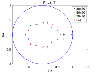
(a) Extrapolated R7 data.

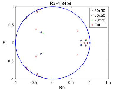
(b) Interpolated R11 data.

Figure 9: Comparison of the first twenty DMD eigenvalues computed from the full data and interpolated/extrapolated data.

For each of the 16 dynamic regimes given by the parameter in Table 1, we compute a DMD basis $\Phi_{i}$ of size $r_{i}=20$, and subsequently assemble the library of regimes $\mathcal{L}$. For the DMD method with augmented basis as introduced in Section 4.3, we use $10$ additional blocks, corresponding to a sequence of $j=10$ sequential time measurements. We consider two possible sensing systems and the corresponding matrices $C$. For both sensing mechanisms, a study with respect to the number of sensors is performed, and the number of sensors used in each test is specified below. In the first sensing system, we sparsely sense from the whole domain by placing point sensors arbitrarily. This serves as a reference, however it is not realistic in many practical applications to assume that sensors can be placed arbitrarily. Thus, in the second system, we consider sensing close to the boundary of the domain, where important boundary effects take place.

Inspired by compressive sensing principles, both our sensing experiments use randomly selected sensors in the corresponding sensing area. Thus, we only use a subset of the sensors in the selected area to robustly classify the regimes.

5.1 Alignment and Coherence Metrics

We use a variety of metrics to quantify the alignment and coherence of the regime library. The metric $\eta$ from (24) can be interpreted as the worst case similarity measure between two subspaces $\Phi_{i}$ and $\Phi_{j}$, since it is based on the spectral norm. We find that for the computed library of regimes, we have $0.95\leq\eta\leq 0.99$. A similar qualitative behavior is seen with $\mu_{B}$ from (31), since it is also based on a spectral norm. Although, as we will see later in this section, $\mu_{B}$ better captures the decay in coherence among regimes when using augmented DMD.

Hence, to get better insight into the coherence of different regimes, we introduce another measure:

$$\gamma_{ij}=\frac{||P_{i}P_{j}||_{F}}{||P_{i}||_{F}||P_{j}||_{F}},$$ (32)

where $P_{i}=\Phi\Phi_{i}^{\dagger}$ for the projection of the full state vector, and $P_{i}=\Theta_{i}\Theta_{i}^{\dagger}$ for the projection subject to measurement $\Theta_{i}=C\Phi_{i}$ onto the boundary. The subscript $F$ indicates the Frobenius norm. Figure 10 shows the measure $\gamma_{ij}$ as defined in equation (32), both for the full projection, and the projection subject to measurement onto the boundary.

In contrast to $\eta$, the measure $\gamma_{ij}$ indicates the fraction of information that is retained on average by projecting a random vector onto subspaces of two different regimes in succession. The diagonal contains ones, and the off diagonal entries are generally decreasing with the off-diagonal index, indicating that only neighboring regimes (in terms of Rayleigh number) share similar features. By definition, the matrices are symmetric. Two clusters of regimes appear, the first one from $Ra=10$ to $Ra=10^{7}$, and the second cluster from $Ra=10^{8}$ to $Ra=8\times 10^{8}$. Note, that the last regime for Rayleigh number $Ra=10^{9}$, resulting in a “chaotic” flow solution, is considerably different from the other regimes. Based on this information, we conjecture that misidentification gets slightly worse within the two clusters when sensing close to the boundary; we also expect to see a confusion matrix similar in structure to Figure 10. The confusion matrix, used to quantify the success of our algorithm, is defined as follows: the $(i,j)th$ entry contains the percentage of tests in which data from regime $i$ is identified as belonging to regime $j$. Tests are performed independently for data from each regime.

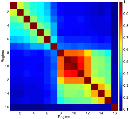
(a) Projection onto full $n$-dimensional space, spanned by DMD basis functions, $P_{i}=\Phi\Phi_{i}^{\dagger}$.

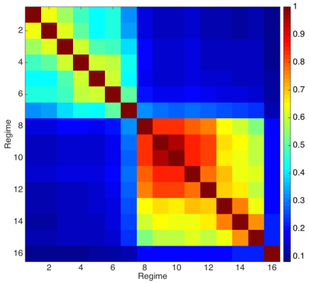
(b) Projection onto the boundary, $P_{i}=\Theta_{i}\Theta_{i}^{\dagger}$ with $\Theta_{i}=C\Phi_{i}$.

Figure 10: The subspace alignment measure $\gamma_{ij}$ from equation (32).

Additionally, we consider the matrix

$$\kappa_{ij}=\frac{||P_{i}X_{j}||_{F}}{||X_{j}||_{F}},\quad i,j=1,\ldots,d,$$ (33)

which measures the energy in the projected subspace compared to the actual data, and allows estimation of $\epsilon$.

Figure 11 shows this measure for the case of full data and boundary data. The measure $\kappa_{ij}$, as defined in equation (33) indicates how much information is preserved by projecting on the basis $\Phi_{i}$, through the projection $P_{i}$. As shown in section 2, DMD modes are in general non-orthonormal vectors that span the same subspace as singular vectors given by the SVD step. Since we picked the top 20 singular vectors to form the DMD subspaces $\Phi_{i}$, we see that the diagonal entries for $\kappa_{ij}$ are mostly above 98%. Additionally, neighboring regimes share similar features; for instance, the projection of the data from regime 3 onto the basis of regime 1 retains a high amount of energy (measured in the Frobenius norm). As before, two groups of regimes appear. For boundary data case, in analogy to the considerations above for the measure $\gamma_{ij}$, the similarity within the two clusters increases and the distinction among the two clusters increases. Consequently, we expect some confusion within the two clusters.

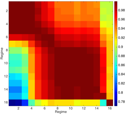
(a) Projection onto full $n$-dimensional space, spanned by DMD basis functions, $P_{i}=\Phi\Phi_{i}^{\dagger}$.

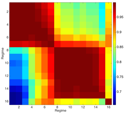
(b) Projection of boundary data $Y_{i}=CX_{i}$ with $P_{i}=\Theta_{i}\Theta_{i}^{\dagger}$ with $\Theta_{i}=C\Phi_{i}$.

Figure 11: The data alignment measure $\kappa_{ij}$ from definition (33).

5.2 Regime Classification

For the first example, we use $10$ velocity sensors, and $50$ temperature sensors. These sensors are placed on the boundary. The velocity is sensed one grid point away from the boundaries. The signal to noise ratio is set to $20$dB, which corresponds to $10\%$ noise in $l_{2}$ sense. The DMD basis is augmented, i.e., we use the time evolution structure as described in Section 4.3 with $j=3$. For each regime, 100 tests are performed, where at each test, a snapshot from a given regime is picked and the best match to one of the 16 regimes is found by projection (15). In Figure 12(a), the confusion matrix for the 16 regimes is plotted. The block with the highest confusion (worst identification) is between regimes R9–R12, corresponding to Rayleigh numbers $1.82\times 10^{8}-2\times 10^{8}$, which is expected since the corresponding Rayleigh numbers are very close to each other.

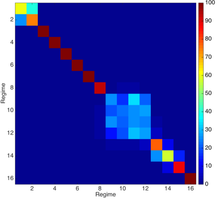
(a) Flow regimes R1–R16.

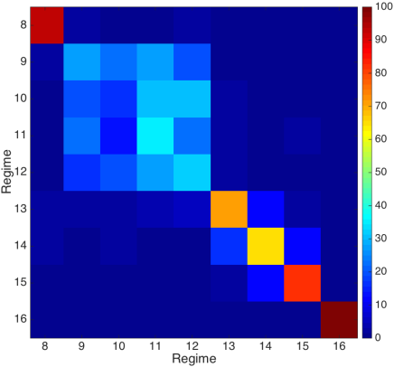
(b) Flow regimes R8–R16.

Figure 12: Confusion matrices from 100 tests for every regime, indicating if the regime was picked correctly, or misclassified. In each test, we selected boundary sensors ($p_{T}=50$ for temperature and $p_{v}=10$ for velocity), and used $j=3$ time measurements with augmented DMD.

From the discussion in Section 3, it is clear that the system has a steady state behavior for Rayleigh numbers corresponding to regimes R1 through R7. Thus, we further focus the analysis and discussion on Rayleigh numbers $Ra=10^{8}$ and higher, corresponding to R8–R16. The results, for another 100 tests for each regime, are presented in more detail in Figure 12(b).

5.2.1 Robustness to out-of-sample data

In the tests reported so far, all available data is used to generate the sparse library, and subsequently, the same data is used for classification. Here, training and testing datasets are separated, to investigate the robustness of the algorithm to unknown data. The testing data is taken from regimes R9, R10, and R11, which correspond to Rayleigh numbers between $1.82\times 10^{8}$ and $1.85\times 10^{8}$. As noted in Section 3, there is a bifurcation of the flow at $Ra\approx 1.82\times 10^{8}$, which has been observed both experimentally, as well as numerically. We performed 600 independent tests, where at each test a flow snapshot (or a series of snapshots for the augmented sensing algorithm) is taken from the test data, and classified using six regimes R8, and R12–R16. One expects the classification of the testing data to match to regime R12, which is closest to the test regime. The signal-to-noise ratio is set to $20$dB, and $p_{v}=10$ flow sensors are used, together with $p_{T}=50$ temperature sensors, all placed on and near the boundary of the unit square. To be precise, the velocity sensors are placed slightly inside the domain, since the velocity is set zero at the boundaries. For better classification performance, and more robustness to noise, the DMD basis is augmented by two blocks, i.e., three time snapshots are taken for classification.

Regime	R8	R12	R13	R14	R15	R16
$Ra$	$10^{8}$	$2\times 10^{8}$	$4\times 10^{8}$	$6\times 10^{8}$	$8\times 10^{8}$	$10^{9}$
Classification	6%	87%	6%	0%	0%	0%

Table 2: Classification performance with out-of-sample sensor data (taken from regimes R9–R12) for six regimes at high Rayleigh numbers. The data is mainly classified as regime R12.

Table 2 reports the classification results. The sensing method is able to match the testing data to the (physically) correct flow patterns. In practice, this is important, since one does not expect the data to repeat itself in a given situation. Hence, the sensing mechanism needs to be able to match data to its “closest” subspace in the library collection.
The regimes R9–R12 correspond to very close parameter values, and their solution subspaces are very similar to each other, as confirmed by looking at Figure 12, and the results of Table 2. Hence, in the remaining analysis, we only consider the six regimes R8, and R12–R16, where R12 is the representative of regimes R9 to R12.

5.2.2 Varying the number of sensors and using more data in time

Next, we numerically study the improvement in classification performance that can be achieved by increasing the number of velocity sensors and time measurements, via the augmented DMD algorithm. In Figure 13, we plot the decay in block coherence measure $\mu_{B}$ with respect to the number of time measurements used in augmented DMD. In Figure 14, we plot the classification performance with $p_{v}=10,15,20,25,30$ velocity sensors, and 10 temperature sensors, all near the boundary. The number of measurements in time used in augmented DMD are $j=1,3,5,10$, and the sensor noise is $10\%$ ($SNR=20$dB). Figure 15 shows the classification results with $30\%$ sensor noise ($SNR=10$ dB). It is evident from these figures that using the augmented DMD approach significantly improves the classification performance. While the value of the sub-coherence $\nu$ is still close to $0.99$, and hence the theoretical guarantee for accurate reconstruction is highly conservative, the classification performance is much better. This improvement is reflected in the decay of $\mu_{B}$ as seen in Figure 13. While we have not focused on optimal sensor placement in this work, this connection between $\mu_{B}$ and classification performance can be used to formulate the problem of optimal sensor placement.

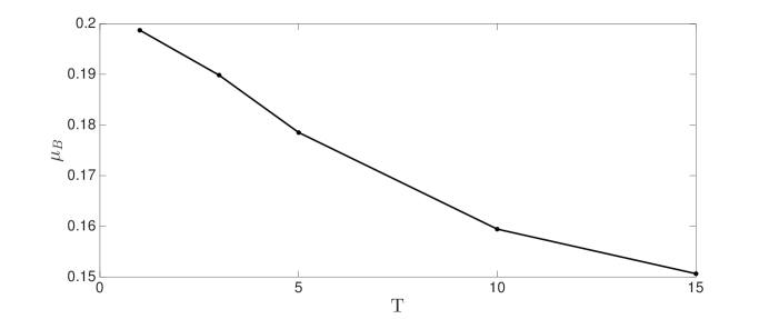
Figure 13: Block coherence measure $\mu_{B}$ as a function of time augmentation $T=j$ using only sensors on the boundary.

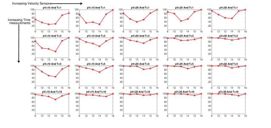
Figure 14: Classification performance with $10\%$ sensor noise (SNR$=20$dB) for different number of near-boundary velocity sensors $p_{v}$, and time measurements $T=j$, with $p_{T}=10$ temperature sensors at the boundary. The performance increases significantly as number of time measurements are increased from 1 to 10, showing the efficacy of augmented DMD.

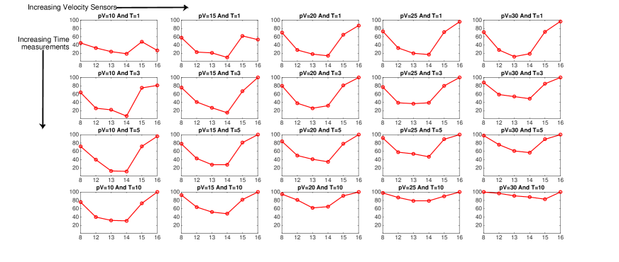
Figure 15: Classification performance with $30\%$ sensor noise (SNR$=10$dB) for different number of near-boundary velocity sensors $p_{v}$, and time measurements $T=j$, with $p_{T}=10$ temperature sensors at the boundary. The performance increases significantly as number of time measurements are increased from 1 to 10, showing the efficacy of augmented DMD.

5.3 Reconstruction in the Library

The goal of this section is to show that the selection of the correct regime basis, i.e., the local model, is important for subsequent state estimation. To do so, we conduct the following simple numerical test for two different cases. We run the system in a specific regime $k^{\star}$. Next, using $p_{T}=10$ temperature sensors and $p_{v}=30$ velocity sensors, we collect snapshots of the corresponding output measurement vector $y_{k^{\star}}(t)\in\mathbb{R}^{70}$. This output vector is then projected onto bases of different regimes from the library $\mathcal{L}_{obs}$, and the resulting coefficients used to reconstruct the full $n$-dimensional state via the DMD library $\mathcal{L}$. By using the simple output-state map inversion

$$x_{i}^{\star}(t)=\Phi_{i}\Theta_{i}^{\dagger}y_{k^{\star}}(t),\quad i\in\{8,12,13,14,15,16\},$$

we then obtain an estimate of the full state vector history.

In Figure 16, we show the reconstruction results using three time measurements from regime R16 (i.e., $k^{*}=16$), and bases from the six regimes. In Figure 17, we show the reconstruction results using three time measurements from regime R15 (i.e., $k^{*}=15$), and bases from the six regimes. Clearly, in both the test cases, the estimates using wrong regimes have significantly more error than estimates using the correct regime.

Of course, this reconstruction is not a proper state reconstruction in the sense of state-space observation. Nevertheless, it shows the importance of selecting the right regime basis. After the correct regime basis has been selected, the corresponding low-dimensional model can be used in the framework of state observation. For instance, by using a Luenberger observer, one can properly estimate the dynamics of the full state vector over time. This part has not been studied in this paper, but will be the focus of our future work.

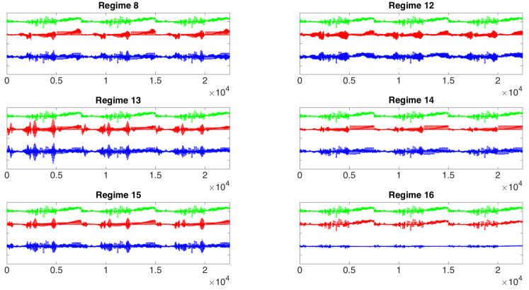
Figure 16: Reconstruction of three consecutive snapshots from a dynamic regime, corresponding to the parameter $Ra=1\times 10^{9}$, in six different regimes, defined via $Ra=\{1\times 10^{8},2\times 10^{8},4\times 10^{8},6\times 10^{8},8\times 10^{8},1\times 10^{9}\}.$ The x-axis is the index of the time augmented state vector. The original signal is shown in green, the reconstructed signal in red and the error is shown in blue. The corresponding relative errors in the Euclidean norm are $\{.0.5895,0.8549,0.7075,0.5346,0.5514,0.1373\}$. The other parameters are: $30\%$ Noise (SNR=$10$dB) , $p_{v}=30$ and $p_{T}=10$ .

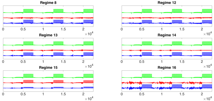
Figure 17: Reconstruction of three consecutive snapshots from a dynamic regime, corresponding to the parameter $Ra=8\times 10^{8}$, in six different regimes, defined via $Ra=\{1\times 10^{8},2\times 10^{8},4\times 10^{8},6\times 10^{8},8\times 10^{8},1\times 10^{9}\}.$ The x-axis is the index of the time augmented state vector. The original signal is shown in green, the reconstructed signal in red and the error is shown in blue. The corresponding relative errors in the Euclidean norm are $\{1.0507,0.9379,0.9447,0.9572,0.3806,1.1602\}$. The other parameters are: $30\%$ Noise ($SNR=10$dB), $p_{v}=30$ and $p_{T}=10$

6 Conclusion

We have introduced a framework for data-driven regime selection in parameter-dependent thermo-fluid systems. Most low-order modeling methods use Galerkin projection-based dynamical reduced models of the infinite-dimensional fluid system. Hence the successful selection of dynamic regimes, and an accurate reconstruction of the corresponding subspace is crucial to the success of such models.

Our framework uses ideas from sparse sensing and exploits the dimensionality reduction performed by reduced order models. In particular, although our model can operate with a variety of dimensionality reduction methods, we use DMD to harness the ability of the Koopman operator to capture the model dynamics. Thus, using a subspace identification method, we can accurately identify the dynamic regime with few sensors distributed near the boundary and few time snapshots.

Our framework uses off-line computation to construct a library of regimes to be used for regime identification. This library comprises of DMD eigenvectors and corresponding eigenvalues for each regime, which capture the subspace in which the state lies under that regime, as well as the dynamics of the state. The dynamical information is used to exploit multiple time measurements, which then increases robustness of the classification with respect to measurement noise and parametric uncertainty.

We numerically demonstrate our approach using a DNS data set of a two dimensional differentially heated cavity flow operating at different Rayleigh numbers. The underlying PDE model is the Boussinesq equation, which captures the dynamics of buoyancy driven flows well, when temperature differences are small. The numerical results suggest that the proposed DMD-based classification method with augmented DMD basis is superior to using only a single-time measurement for classification.

Of course, our work is only a small step towards our goal, namely low-order sensing and control models for complicated parametric thermo-fluid systems. Parametric DMD [52] is one recent attempt to explicitly take into account the effect of parameters in the DMD framework. State estimation has not been studied here, and will be the focus of our future report. Indeed, using the identified low-order model and the correct regime it is possible to construct a stabilized low-order model and correctly identify its parameters using data-driven learning techniques [7, 6]. Combining the DMD model with low-order Galerkin models is another promising direction [58]. These low dimension models can then be used for state observation, e.g., using Luenberger observers.

Regime construction is currently a manual process, understood only for a few well-established systems. Automated optimal labeling and sorting of data into different regimes, according to some measures such as those discussed in this paper, would remove the need for manual construction of regimes.

Another avenue of further research suggested by this work is the connection between nonlinear systems and sparsity theory. While some basic results in observability, controllability and state estimation for linear systems with sparse states are already known [61, 51], our results suggest that this framework could be extended to nonlinear systems via the DMD.

References

- [1] O. Akanyeti, R. Venturelli, F. Visentin, L. Chambers, W. M. Megill and P. Fiorini “What information do Kármán streets offer to flow sensing?” In Bioinspiration & biomimetics 6.3 IOP Publishing, 2011, pp. 036001
- [2] A. C. Antoulas “Approximation of Large-Scale Dynamical Systems (Advances in Design and Control)” Philadelphia, PA, USA: Society for IndustrialApplied Mathematics, 2005
- [3] N. Aubry, P. Holmes, J.L. Lumley and E. Stone “The dynamics of coherent structures in the wall region of a turbulent boundary layer” In Journal of Fluid Mechanics 192 Cambridge Univ Press, 1988, pp. 115–173
- [4] Shervin Bagheri “Koopman-mode decomposition of the cylinder wake” In Journal of Fluid Mechanics 726 Cambridge Univ Press, 2013, pp. 596–623
- [5] Z. Bai, T. Wimalajeewa, Z. Berger, G. Wang, M. Glauser and P.K. Varshney “Low-Dimensional Approach for Reconstruction of Airfoil Data via Compressive Sensing” In AIAA Journal American Institute of AeronauticsAstronautics, 2014, pp. 1–14
- [6] M. Benosman “Learning-Based Adaptive Control, An Extremum Seeking Approach : Theory and Applications” Elsevier, 2016
- [7] M. Benosman, B. Kramer, P. Grover and P. Boufounos “Learning-based Reduced Order Model Stabilization for Partial Differential Equations: Application to the Coupled Burgers Equation” In Proceedings of the 2016 American Control Conference, 2016
- [8] P. Boufounos, G. Kutyniok and H. Rauhut “Sparse recovery from combined fusion frame measurements” In IEEE Trans. Info. Theory 57.6, 2011, pp. 3864–3876 DOI: 10.1109/TIT.2011.2143890
- [9] I. Bright, G. Lin and J. N. Kutz “Compressive sensing based machine learning strategy for characterizing the flow around a cylinder with limited pressure measurements” In Physics of Fluids (1994-present) 25.12 AIP Publishing, 2013, pp. 127102
- [10] Steven L Brunton, Joshua L Proctor, Jonathan H Tu and J Nathan Kutz “Compressed Sensing and Dynamic Mode Decomposition” In Journal of Computational Dynamics 2.2, 2015
- [11] Steven L Brunton, Jonathan H Tu, Ido Bright and J Nathan Kutz “Compressive sensing and low-rank libraries for classification of bifurcation regimes in nonlinear dynamical systems” In SIAM Journal on Applied Dynamical Systems 13.4 SIAM, 2014, pp. 1716–1732
- [12] Marko Budišić, Ryan Mohr and Igor Mezić “Applied Koopmanism” In Chaos: An Interdisciplinary Journal of Nonlinear Science 22.4 AIP Publishing, 2012, pp. 047510
- [13] J. A. Burns, J. T. Borggaard, E. Cliff and L. Zietsman “An Optimal Control Approach to Sensor/Actuator Placement for Optimal Control of High Performance Buildings” In International High Performance Buildings Conference, 2012
- [14] E. J. Candès, J. Romberg and T. Tao “Robust uncertainty principles: Exact signal reconstruction from highly incomplete frequency information” In Information Theory, IEEE Transactions on 52.2 IEEE, 2006, pp. 489–509
- [15] E. J. Candès and T. Tao “Near-optimal signal recovery from random projections: Universal encoding strategies?” In Information Theory, IEEE Transactions on 52.12 IEEE, 2006, pp. 5406–5425
- [16] Emmanuel J Candès “Compressive sampling” In Proceedings oh the International Congress of Mathematicians: Madrid, August 22-30, 2006: invited lectures, 2006, pp. 1433–1452
- [17] K. K. Chen, J. H. Tu and C. W. Rowley “Variants of dynamic mode decomposition: boundary condition, Koopman, and Fourier analyses” In Journal of nonlinear science 22.6 Springer, 2012, pp. 887–915
- [18] D. L. Donoho “Compressed sensing” In Information Theory, IEEE Transactions on 52.4 IEEE, 2006, pp. 1289–1306
- [19] Y. C Eldar, P. Kuppinger and H. Bolcskei “Block-sparse signals: Uncertainty relations and efficient recovery” In Signal Processing, IEEE Transactions on 58.6 IEEE, 2010, pp. 3042–3054
- [20] H. Fang, R. Sharma and R. Patil “Optimal sensor and actuator deployment for HVAC control system design” In American Control Conference (ACC), 2014, 2014, pp. 2240–2246 IEEE
- [21] Gary Froyland and Kathrin Padberg “Almost-invariant sets and invariant manifolds, connecting probabilistic and geometric descriptions of coherent structures in flows” In Physica D: Nonlinear Phenomena 238.16 Elsevier, 2009, pp. 1507–1523
- [22] Pierre Gaspard and Shuichi Tasaki “Liouvillian dynamics of the Hopf bifurcation” In Physical Review E 64.5 APS, 2001, pp. 056232
- [23] R. Ghosh and Y. Joshi “Proper Orthogonal Decomposition-Based Modeling Framework for Improving Spatial Resolution of Measured Temperature Data” In Components, Packaging and Manufacturing Technology, IEEE Transactions on 4.5, 2014, pp. 848–858 DOI: 10.1109/TCPMT.2013.2291791
- [24] Michael D Graham and Ioannis G Kevrekidis “Alternative approaches to the Karhunen-Loeve decomposition for model reduction and data analysis” In Computers & chemical engineering 20.5 Elsevier, 1996, pp. 495–506
- [25] Piyush Grover, Shane D Ross, Mark A Stremler and Pankaj Kumar “Topological chaos, braiding and bifurcation of almost-cyclic sets” In Chaos: An Interdisciplinary Journal of Nonlinear Science 22.4 AIP Publishing, 2012, pp. 043135
- [26] George Haller “Lagrangian coherent structures” In Annual Review of Fluid Mechanics 47 Annual Reviews, 2015, pp. 137–162
- [27] Maziar S Hemati, Matthew O Williams and Clarence W Rowley “Dynamic mode decomposition for large and streaming datasets” In Physics of Fluids (1994-present) 26.11 AIP Publishing, 2014, pp. 111701
- [28] P. Holmes, J. L. Lumley and G. Berkooz “Turbulence, coherent structures, dynamical systems and symmetry” Cambridge university press, 1998
- [29] M. Hortmann, M. Peric and G. Scheuerer “Finite volume multigrid prediction of laminar natural convection: Bench-mark solutions” In International journal for numerical methods in fluids 11.2 Wiley Online Library, 1990, pp. 189–207
- [30] “http://nek5000.mcs.anl.gov/” URL: http://nek5000.mcs.anl.gov/
- [31] M. R Jovanović, P. J Schmid and J. W Nichols “Sparsity-promoting dynamic mode decomposition” In Physics of Fluids (1994-present) 26.2 AIP Publishing, 2014, pp. 024103
- [32] Oliver Junge, Jerrold E Marsden and Igor Mezic “Uncertainty in the dynamics of conservative maps” In Decision and Control, 2004. CDC. 43rd IEEE Conference on 2, 2004, pp. 2225–2230 IEEE
- [33] Yueheng Lan and Igor Mezić “Linearization in the large of nonlinear systems and Koopman operator spectrum” In Physica D: Nonlinear Phenomena 242.1 Elsevier, 2013, pp. 42–53
- [34] Patrick Le Quéré and Masud Behnia “From onset of unsteadiness to chaos in a differentially heated square cavity” In Journal of fluid mechanics 359 Cambridge Univ Press, 1998, pp. 81–107
- [35] D. M. Luchtenburg, B. R. Noack and M. Schlegel “An introduction to the POD Galerkin method for fluid flows with analytical examples and MATLAB source codes” In Institut für Strömungsmechanik und Technische Akustik, TU Berlin, 2009
- [36] N. Massarotti, P. Nithiarasu and O. C. Zienkiewicz “Characteristic-based-split (CBS) algorithm for incompressible flow problems with heat transfer” In International Journal of Numerical Methods for Heat and Fluid Flow 8.8, 1998, pp. 969–990
- [37] I. Mezić “Analysis of fluid flows via spectral properties of the Koopman operator” In Annual Review of Fluid Mechanics 45 Annual Reviews, 2013, pp. 357–378
- [38] Igor Mezić “Spectral properties of dynamical systems, model reduction and decompositions” In Nonlinear Dynamics 41.1-3 Springer, 2005, pp. 309–325
- [39] Ryan Mohr and Igor Mezić “Construction of eigenfunctions for scalar-type operators via Laplace averages with connections to the Koopman operator” In arXiv preprint arXiv:1403.6559, 2014
- [40] B. R. Noack, M. Schlegel, M. Morzyński and G. Tadmor “System reduction strategy for Galerkin models of fluid flows” In International Journal for Numerical Methods in Fluids 63.2 Wiley Online Library, 2010, pp. 231–248
- [41] S. Omatu, S. Koide and T. Soeda “Optimal sensor location problem for a linear distributed parameter system” In Automatic Control, IEEE Transactions on 23.4 IEEE, 1978, pp. 665–673
- [42] S A Orzsag “On the elimination of aliasing in finite-difference schemes by filtering high-wavenumber components” In Journal of the Atmospheric sciences 28, 1971, pp. 1704
- [43] Jan Östh, Bernd R Noack, Siniša Krajnović, Diogo Barros and Jacques Borée “On the need for a nonlinear subscale turbulence term in POD models as exemplified for a high-Reynolds-number flow over an Ahmed body” In Journal of Fluid Mechanics 747 Cambridge Univ Press, 2014, pp. 518–544
- [44] S Paolucci “Direct simulation of two-dimensional turbulent natural convection in an enclosed cavity” In Journal of Fluid Mechanics 215, 1990, pp. 229–262
- [45] Anthony T Patera “A spectral element method for fluid dynamics: laminar flow in a channel expansion” In Journal of computational Physics 54.3 Elsevier, 1984, pp. 468–488
- [46] Joshua L Proctor, Steven L Brunton and J Nathan Kutz “Dynamic mode decomposition with control” In SIAM Journal on Applied Dynamical Systems 15.1 SIAM, 2016, pp. 142–161
- [47] Shane D Ross and Phanindra Tallapragada “Detecting and exploiting chaotic transport in mechanical systems” In Applications of Chaos and Nonlinear Dynamics in Science and Engineering-Vol. 2 Springer, 2012, pp. 155–183
- [48] C.W Rowley, I. Mezić, S. Bagheri, P. Schlatter and D.S Henningson “Spectral analysis of nonlinear flows” In Journal of Fluid Mechanics 641 Cambridge University Press, 2009, pp. 115–127
- [49] E. Samadiani, Y. Joshi, H. Hamann, M. K. Iyengar, S. Kamalsy and J. Lacey “Reduced order thermal modeling of data centers via distributed sensor data” In Journal of Heat Transfer 134.4 American Society of Mechanical Engineers, 2012, pp. 041401
- [50] Omer San and Jeff Borggaard “Basis Selection and Closure for POD Models of Convection Dominated Boussinesq Flows” In Mathematical Theory of Networks and Systems, 21st International Symposium on, 2014, pp. 132–139
- [51] Aswin C Sankaranarayanan, Pavan K Turaga, Rama Chellappa and Richard G Baraniuk “Compressive acquisition of linear dynamical systems” In SIAM Journal on Imaging Sciences 6.4 SIAM, 2013, pp. 2109–2133
- [52] Taraneh Sayadi, Peter J Schmid, Franck Richecoeur and Daniel Durox “Parametrized data-driven decomposition for bifurcation analysis, with application to thermo-acoustically unstable systems” In Physics of Fluids (1994-present) 27.3 AIP Publishing, 2015, pp. 037102
- [53] P. J. Schmid “Dynamic mode decomposition of numerical and experimental data” In Journal of Fluid Mechanics 656 Cambridge Univ Press, 2010, pp. 5–28
- [54] S Sirisup and GE Karniadakis “A spectral viscosity method for correcting the long-term behavior of POD models” In Journal of Computational Physics 194.1 Elsevier, 2004, pp. 92–116
- [55] Sirod Sirisup, George Em Karniadakis, Dongbin Xiu and Ioannis G Kevrekidis “Equation-free/Galerkin-free POD-assisted computation of incompressible flows” In Journal of Computational Physics 207.2 Elsevier, 2005, pp. 568–587
- [56] Mark A Stremler, Shane D Ross, Piyush Grover and Pankaj Kumar “Topological chaos and periodic braiding of almost-cyclic sets” In Physical review letters 106.11 APS, 2011, pp. 114101
- [57] J. A. Taylor and M. N. Glauser “Towards practical flow sensing and control via POD and LSE based low-dimensional tools” In Journal of fluids engineering 126.3 American Society of Mechanical Engineers, 2004, pp. 337–345
- [58] G. Tissot, L. Cordier, N. Benard and B. R. Noack “Model reduction using Dynamic Mode Decomposition” In Comptes Rendus Mécanique 342.6 Elsevier, 2014, pp. 410–416
- [59] Jonathan H Tu, Clarence W Rowley, Dirk M Luchtenburg, Steven L Brunton and J Nathan Kutz “On Dynamic Mode Decomposition: Theory and Applications” In Journal of Computational Dynamics 1.2, 2014, pp. 391–421
-
[60]
S. Volkwein
“Proper Orthogonal Decomposition: Theory and Reduced-Order
Modelling”, Lecture Notes, University of Konstanz, available at
http://www.math.uni-konstanz.de/numerik/personen/volkwein/teaching/scripts.php, 2013 URL: http://www.math.uni-konstanz.de/numerik/personen/volkwein/teaching/scripts.php - [61] M. B. Wakin, B. M. Sanandaji and T. L. Vincent “On the observability of linear systems from random, compressive measurements” In Decision and Control (CDC), 2010 49th IEEE Conference on, 2010, pp. 4447–4454 IEEE
- [62] K. Willcox “Unsteady flow sensing and estimation via the gappy proper orthogonal decomposition” In Computers & fluids 35.2 Elsevier, 2006, pp. 208–226
- [63] Matthew O Williams, Ioannis G Kevrekidis and Clarence W Rowley “A Data–Driven Approximation of the Koopman Operator: Extending Dynamic Mode Decomposition” In Journal of Nonlinear Science 25.6 Springer US, 2015, pp. 1307–1346