What did Erwin Mean?
The Physics of Information from the Materials Genomics of Aperiodic Crystals & Water to Molecular Information Catalysts & Life

Abstract

Erwin Schrödinger famously and presciently ascribed the vehicle transmitting the hereditary information underlying life to an ‘aperiodic crystal’. We compare and contrast this, only later discovered to be stored in the linear biomolecule DNA, with the information bearing, layered quasi-one-dimensional materials investigated by the emerging field of chaotic crystallography. Despite differences in functionality, the same information measures capture structure and novelty in both, suggesting an intimate coherence between the information character of biotic and abiotic matter—a broadly applicable physics of information. We review layered solids and consider three examples of how information- and computation-theoretic techniques are being applied to understand their structure. In particular, (i) we review recent efforts to apply new kinds of information measures to quantify disordered crystals; (ii) we discuss the structure of ice I in information-theoretic terms; and (iii) we recount recent experimental results on tris(bicyclo[2.1.1]hexeno)benzene TBHB), showing how an information-theoretic analysis yields additional insight into its structure. We then illustrate a new Second Law of Thermodynamics that describes information processing in active low-dimensional materials, reviewing Maxwell’s Demon and a new class of molecular devices that act as information catalysts. Lastly, we conclude by speculating on how these ideas from informational materials science may impact biology.

1 Introduction

To account for the ‘special properties’ of life—e.g., movement, metabolism, reproduction, development—the prevailing wisdom from the time of Aristotle into the 19th century was that organic matter differed in some fundamental way from inorganic matter. While this notion, called vitalism, may seem quaint to 21st century scientists, it held sway until the chemist Friedrich Wöhler showed that, unexpectedly, a known organic compound, urea, could be artificially synthesized from cyanic acid and ammonia [1]. This fabrication process, while different than that used in biological systems, nonetheless served as an important clue that the divide between living and nonliving matter was not absolute. Abiotic processes could make substances theretofore only encountered in biologically derived materials. Additionally, we see that—and not for the last time—results obtained from one discipline, chemistry, have had important consequences in another, biology. This confluence of diverse avenues of inquiry coalescing into an ever larger conceptual picture of Nature is, of course, an oft-repeated theme in the sciences. Other famous examples include Newton’s discovery that the motion of celestial bodies, such as the moon planets, and that of terrestrial ones under the influence of gravity, such as the proverbial apple, both are manifestations of a universal law of gravitational attraction; James Clerk Maxwell’s unification of electricity and magnetism into his famous equations; and James Prescott Joule’s demonstration that the caloric was nothing but energy by another name, now formalized in the First Law of Thermodynamics. Indeed, E. O. Wilson takes the extreme position that all human knowledge, from the most concrete of the sciences to the least precise of the liberal arts, is ultimately interlinked [2].

We need not go quite so far as Wilson. It is enough for our purposes to realize that while ‘abiotic’ sciences such as physics, chemistry, astronomy, and geology share obvious strong interconnections, biology has remained relatively aloof. This is not to say that biology has not benefited greatly from knowledge transferred to it from other physical sciences. In addition to the urea example above, note that metabolism is at its core a question of the utilization and transformation of energy—a notion made concrete and operational in physics. And too, biology has benefited tremendously from techniques and discoveries made in other sciences. Indeed, in 1937 Max Delbrück (Nobel Prize Physiology or Medicine 1969) adapted his training in astrophysics and theoretical physics to probe gene susceptibility to mutations, stimulating physicists’ interest in biology and establishing molecular biology. More familiar, though, it was the infamous X-ray diffraction image known as ‘photograph 51’ from the lab of Rosalind Franklin that provided a key insight leading geneticist James Watson and physicist Francis Crick (Nobel Prize in Physiology or Medicine 1962) to propose the double helical structure of DNA [3]. Despite the above, biology is clearly the least well integrated in the family of sciences. We can speculate that the sheer complexity of life and the novel phenomena it displays are at least partially responsible for this. Even one of the most basic organisms, Mycoplasma genitalium, has genome of ‘only’ $580,070$ base pairs [4]. Biology is complicated.

And it is perhaps due to this complication that the mathematical ‘sciences’ have made their least impact in theoretical biology. By and large, the advanced mathematical techniques that saturate any theoretical physics text find no counterpart in biology texts. There is one area, however, where arguably biology has outpaced her sister sciences: the incorporation of information theory[5, 6] into the description of physical systems. And, we will suggest that biology has carved a conceptual path that abiotic physical sciences would do well to emulate. Before we move too far ahead, though, let’s start at the turn of the 20th century and visit one of the many revolutionary advances that ushered in the era of ‘modern’ physics and that remains today a key probe of molecular biological structure.

2 Structure, Aperiodic Crystals, and Information

The immense conceptual advances in physics made in the first third of the 20th century are legion, but here we focus on the contributions to the structure of matter. While it is Max von Laue (Nobel Prize Physics 1914) that is credited with the discovery of the diffraction of X-rays by crystals, it is the father and son team, Sir William Henry Bragg and William Lawrence Bragg (Nobel Prize Physics 1915), that receive much of the credit for exploiting it as a tool to determine crystal structure. For a periodic repetition of some pattern, as one might find in the simple crystals such as NaCl, the diffraction pattern is dominated by very strong reflections at particular angles, called Bragg reflections. Much weaker diffuse scattering is known to occur between the Bragg reflections and had been observed as early as 1912 by Walter Friedrich. While this diffuse scattering can be explained by the thermal motion of the constituent atoms, it could genuinely be a harbinger of deviations from perfect periodic order. But the assumption of periodicity greatly simplifies the analysis of diffraction patterns, and the early years of crystallography were marked with enormous success in solving for the periodic structures that seemed so common. Indeed, it may be argued that this research program so successful in describing a particular kind of structure—periodic structure, “the infinite repetition in space of identical structural units”—came at the cost of developing alternate theoretical tools.

On the biology front, cognizant of Delbrück’s results on mutations, the prominent physicist Erwin Schrödinger (Nobel Prize Physics 1933) was busy considering life from a physics point-of-view. In his now classic 1944 book, What is Life? [7], Schrödinger introduces two concepts that are of interest to us here. The first is negentropy, or the entropy that an organism exports to its surroundings to keep its internal entropy low. If one views entropy as a measure of disorder, then the Second Law of Thermodynamics makes it clear that for an organism to maintain some structure, it must rid itself of the disorder that accompanies life-maintaining processes. The second, and equally important, is the idea that the hereditary mechanism that must exist so that traits of individuals can be passed to offspring could be housed in what he called an aperiodic crystal. Although H. L. Muller made a similar proposal over twenty years previous, it was Schrödinger’s advocacy that captured the imagination of Crick and Watson to seriously investigate this possibility. Schrödinger’s aperiodic crystal was some material substrate, perhaps a molecule, that lacked strict periodicity. The reason for this is that exact repetition of a motif, in other words a crystal, is information poor—too poor to carry heredity. Without some unpredictability, or novelty, nothing new is learned and communicated. It is remarkable that Schrödinger made this prediction before a quantitative understanding of information was articulated.

In 1947, three physicists from Bell Telephone Laboratories, John Bardeen, Walter Brattain, and William Shockley (Nobel Prize Physics 1956) invented a small device that revolutionized the design of electrical circuits: the transistor, which ushered in the era of electronics. It’s significance was immediately recognized and a press release was duly issued the next year. Yet, arguably [8], this was only the second most important announcement to come out of Bell Labs in 1948. The first came from a thirty-two year-old mathematician, engineer, and cryptographer, Claude E. Shannon, in the form of a paper in the Bell System Technical Journal with the unassuming title “A Mathematical Theory of Communication" [5].

Shannon’s main premise is that information is a degree of surprise. Given an information source $X$—a set of messages $\{x\}$ that occur with probabilities $\{\Pr(x)\}$—an individual message’s self-information is $\operatorname{H}(x)=-\log_{2}\Pr(x)$. Thus, predictable events ($\Pr(x)=1$) are not informative—$\operatorname{H}(x)=0$, since they are not surprising. Wholly unpredictable events, such as the flips of a fair coin, are highly informative: $\operatorname{H}(\text{Heads})=-\log_{2}\tfrac{1}{2}=1$. When using logarithms base $2$ the information unit is a bit or binary digit. Shannon’s first major result was to show that the average self-information, what he called the entropy paralleling Boltzmann and Gibbs in vocabulary and notation, $\operatorname{H}[X]=-\sum_{x\in X}\Pr(x)\operatorname{H}(x)$ measures how compressible a source’s messages are. However, quantifying information was simply preliminary to Shannon’s main motivation. Working for the Bell Telephone Company, a communications enterprise, his main goal was to lay out operational constraints for communicating information over noisy, error-prone transmission equipment, which he formalized as a communication channel. The result was his most famous and far-reaching result: As long as the source entropy is less that the channel’s transmission capacity—$\operatorname{H}[X]<\mathcal{C}$—then, even if errors are introduced there is a way to encode the source messages such that the receiver observing the noisy channel output can exactly reconstruct the original messages. This single result is key to almost all communication technologies that drive today’s modern economies.

Shannon himself was rather careful to distance his quantitative theory on the amount of information in a source from discussions of that information’s meaning or semantic content [9]. His goal was the operational result just recounted that did not require knowing what information was being communicated. However, as we will explain, his measure of information and its semantics turn out to provide a central and quantitative tool for understanding the organization of materials that are more than periodic crystals—materials that are not regular repetitions of identical unit cells. We call this application of Shannon’s information theory to material structure “chaotic crystallography”, for reasons that will become evident.

What kinds of materials are not crystals? An obvious class is those in which atoms of random kinds are randomly placed in space. The resulting dichotomy—materials are either periodic or random—is too simple a view. There is a spectrum. A first example, one controversial in its time, came in the discovery of quasi-crystals [10]: Metals with long-range orientational order, an icosahedral phase, but no translational symmetry. This fell so far outside of the periodic-random dichotomy that it was some years after experimental detection that quasi-crystals were widely accepted (Nobel Prize in Chemistry 2011).

We now know that the spectrum of material structures between periodic crystals and amorphous materials is populated by much more than quasi-crystals. First are the so-called aperiodic crystals that exhibit sharp diffraction peaks, but not lattice periodicity  [11]. The mathematics of such aperiodic orders has blossomed [12]. Many disordered materials, however, exhibit broadband diffraction patterns but also have a large degree of organization. These are what we now call chaotic crystals. The aperiodic crystals, by way of comparison, are seen to lie in the narrow boundary region between periodic and chaotic crystal materials.

Given this wide spectrum, one needs tools that readily describe processes that range from periodicity to randomness and capture the intermediate semi-ordered, semi-disordered structures. Information theory is one of those tools. We will describe how it applies to material structure, forming the endeavor of chaotic crystallography. A compelling insight is that though we start with a focus just on surprise and prediction, we are led to novel notions of structure, partial symmetries, and information storage.

3 From Information Measures to Structure

Although fundamental to the practice of science, a thorough understanding of the information obtained from individual measurements has only recently been examined in detail [13, 14]. The key issues at hand are easily stated: Given a history of such measurements, how much does one learn from any particular observation? How much of the past is useful for predicting the results of future measurements? To what degree is a measurement simply randomness, and not structure? How much information obtained in the present is transmitted to the future? Perhaps not surprisingly, considering these questions in the light of information theory [6] revealed a number of new computational and informational measures that give important insights into how correlations are manifested in different kinds of structure.

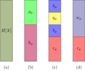
Figure 1: Dissecting the information $\operatorname{H}[X]$ learned from a measurement of a single random variable $X$. (Figure from James et al. [13], used with permission.)

As noted above, the workhorse of information theory is the Shannon entropy [5] of a random variable $X$: $\operatorname{H}(X)=-\sum_{x\in X}\Pr(x)\log_{2}\Pr(x)$, where the $x$ are the possible realizations of the discrete variable $X$ and $\Pr(x)$ is the probability of observing $x$. While Shannon entropy has many interpretations, most useful here is that it is the average amount of information an observation reveals when measuring that variable. Real measurements are often sequential in time and one might expect that there are correlations between measurements. The extension of the Shannon entropy to a series of measurements follows naturally by replacing the single random variable $X$ with the sequence $X_{1},X_{2},\dots X_{L}$ of random variables—often written $X^{L}$—and the realization of a single measurement $x$ by the series of measurements $x_{1},x_{2},\dots x_{L}$, the latter conveniently denoted $x^{L}$. Thus, by considering successively longer pasts —$X_{-1}$, then $X_{-2}X_{-1}$, and so on—one can quantify how less uncertain a measurement of $X_{0}$ is. Or, stated differently, we can quantify how much knowledge of the past reduces the information learned in the present: $\operatorname{H}[X_{0}]\geq\operatorname{H}[X_{0}|X_{-1}]\geq\operatorname{H}[X_{0}|X_{-1},X_{-2}]\geq\ldots$, where we introduced the conditional Shannon entropy $\operatorname{H}[X|\cdot]$. It is also useful to consider the entropy rate ${h_{\mu}}$, the information learned on average per observation, having seen an infinite past: ${h_{\mu}}=\operatorname{H}[X_{0}|\ldots X_{-3}X_{-2}X_{-1}]$.

Since information theory was originally developed in the context of communication, imagined as a temporal progression of symbols, a natural notion of past, present, and future permeated the theory. Operating under this prejudice introduced a preferred arrow of time. As a consequence, the utility of conditioning current measurements, or observed symbols, on future observations was not obvious. From a mathematical point of view, of course, there is no inherent impediment to doing this. However, replacing a time series by a spatial one lifts the directional prejudice, opening a way to identify other measures of information that treat the past and future on equal footing [13, 15, 16, 17, 18].

As an example, consider a single measurement of the random variable $X$. The theoretical maximum amount of information that one can possibly learn is just $\operatorname{H}[X]$, see Fig. (1a). However, if there are correlations or regularities in the data, some of this could have been anticipated from previous observations. Let us call this part the redundancy rate ${\rho_{\mu}}=\operatorname{I}[X_{0}:\ldots X_{-3}X_{-2}X_{-1}]$—the mutual information between the present $X_{0}$ and the past $\ldots X_{-3}X_{-2}X_{-1}$. The other part of the information could not be anticipated; it truly is random and is just ${h_{\mu}}$. Thus, the amount of information available in a measurement naturally decomposes into these two parts, as shown in Fig. (1b).

However, further conditioning yields further decomposition of each of these. First, the random portion ${h_{\mu}}$ breaks into two parts: the ephemeral information rate ${r_{\mu}}$ and the bound information rate ${b_{\mu}}$. The ephemeral information rate ${r_{\mu}}=\operatorname{H}[X_{0}|\ldots X_{-3}X_{-2}X_{-1},X_{1}X_{2}X_{3}\ldots]$ is the information that exists only in the present. It is not predictable from the past nor is it communicated to the future. Existing only in the present, it is ephemeral. The bound information rate ${b_{\mu}}=\operatorname{I}[X_{0}:X_{1}X_{2}X_{3}\ldots|\ldots X_{-3}X_{-2}X_{-1}]$ is the information shared between the present and future, but is not in the past. As such, it measures the rate at which spontaneously generated information (${h_{\mu}}$) is actively stored by a system. Second, the redundancy rate also breaks into two parts, the first again being ${b_{\mu}}$ and a second part called the enigmatic information rate ${q_{\mu}}$. The latter is three-way mutual information $\operatorname{I}[\ldots X_{-3}X_{-2}X_{-1}:X_{0}:X_{1}X_{2}X_{3}\ldots]$ shared between the past, the present, and the future.

The net “decomposition” of the information $\operatorname{H}[X_{0}]$ in a single measurement is illustrated in Fig. (1c). This is only a sampling of the possible ways that information can be semantically partitioned between the past, present, and future. Figure (1d), for example, is a decomposition into dissipated ${r_{\mu}}$ and useful information $w_{\mu}$. Moreover, other additional measures, discussed by James et al. [13, 14, 19], have been defined and explored. Importantly, they now can all be analytically calculated from a process’s $\epsilon$-machine [20, 21], once that is in hand.

4 Chaotic Crystallography

Armed with this new arsenal of structural information measures, a detailed, quantitative picture of how information is shared between the past, present, and future is made plain. With these in mind, intrinsic computation is defined as how systems store, organize, and transform historical and spatial information [22, 23]. Different processes may have quantitatively and qualitatively different kinds of intrinsic computation, and understanding these differences gives insight into how a system is structured [24].

Chaotic crystallography (ChC) [21, 25, 26, 27, 28, 29, 30] then is the application of these information- and computation-theoretic methods to discover and characterize structure in materials. It reinterprets the time axis, used above for pedagogical reasons, for a one-dimension spatial coordinate along some direction in a material. The choice of the name is intended to be evocative: we retain the term “crystallography” to emphasize continuity with past goals of understanding material structure; and we introduce the term “chaotic” to associate this new approach with notions of disorder, complexity, and information processing. Using chaotic crystallography we can describe the ways in which this information decomposition quantitatively captures crystal structure—distinguishing structure that might be expected, i.e., repetitive periodic structure, from that structure not expected, i.e., faulting structure.

4.1 Material Informatics of Faults and Defects

Since classical crystallography [31, 32, 33] largely concentrates on periodic structures, it encounters difficulty classifying structures that do not fit this paradigm. Most efforts have centered on describing how a crystal, that presumably could have been perfectly ordered, falls short of this ideal. For example, in close-packed structures, Frank [34] distinguished two kinds of layer faults: intrinsic and extrinsic. For intrinsic faults, each layer in the material may be thought of as belonging to one of two crystal structures: either that to the left of the fault or that to the right. It is as if two perfect, undefected crystals are glued together and the interface between them is the fault. In contrast, it may be that a particular layer cannot be thought of as a natural extension of the crystal structure on either side of the fault. These are extrinsic faults. Another classification scheme has its origins in the mechanism that produced the fault. In close-packed structures, commonly encountered faults include growth faults—i.e., those that occur during the crystal growth process; deformation faults—which are often associated with some post-formation mechanical stress to the crystal; and layer-displacement faults—which can occur by diffusion between adjacent layers. As each is defined in relation to its parent crystal structure, each kind of crystal structure typically has its own distinctive morphology for each kind of fault.

The result is a confusing menagerie of stacking sequences that deviate from the normal. This collection may not be exhaustive, depending on how large of a neighborhood one considers nor may particular sequences be unambiguously assigned to a particular kind of fault structure. Indeed, in the event that there are multiple kinds of faults, or multiple mechanisms for producing faults, an attempted analysis of the fault structure may be indeterminate [26]. Faulting may also be classified in terms of how faults are spatially related to each other. The absence of correlation between faults implies random faulting. Alternatively, the presence of a fault can influence the probability of finding another fault nearby. This latter phenomenon is called nonrandom faulting and is not uncommon in heavily defected specimens. Lastly, in some materials faults appear to be regularly interjected into the specimen, and this is referred to as periodic faulting. Screw dislocations are thought to be a common cause for these latter faults [35].

Figure 2: Information diagram showing the information anatomy of $\operatorname{H}[X_{0}]$ in the context of the full spatial stacking of layers in a chaotic crystal. Let $X_{0}$ be the layer of interest, $X_{:0}$ be an arbitrarily long but finite section of the specimen to the left of $X_{0}$, and $X_{1:}$ similarly be an arbitrarily long but finite section of the specimen to the right of $X_{0}$. The left $X_{:0}$ partitions $\operatorname{H}[X_{0}]$ into two pieces: $h_{\mu}$ and $\rho_{\mu}$. The right $X_{1:}$ then partitions those into $r_{\mu}$, two $b_{\mu}$s and $q_{\mu}$. (Recall Fig. 1 which decomposed only $\operatorname{H}[X_{0}]$.) This leaves a component $\sigma_{\mu}$, the elusive information, that is shared by the left and right, but is not in the present layer. When positive, it indicates that not all of the correlation between left and right half-configurations is contained in locally and so there are internal hidden mechanisms that carry the correlation [19]. (Figure from James et al. [13]. Used with permission.)

These phenomenological categorizations, while often helpful and sensible, especially for weakly faulted crystals, are not without difficulties. First, it is clear that each is grounded in the assumption that the native, or ideal, state of the specimen must be a periodic structure. This bias, perhaps not intentionally, relegates nonperiodic stacking to less stature, as is evident in the use of the term “fault”. It may be rather that disorder is the natural state of the specimen [36], in which case employing a framework that incorporates this feature of matter upfront will prove more satisfactory. In fact, it is not even clear that periodic order should be the ground state for many kinds materials, even for those with finite-range interactions and in the absence of fine-tuning of energetic coupling parameters between layers [37], as is found in axial next-nearest neighbor Ising (ANNNI) models [38]. Second, an analysis of the stacking structure based on these categories may not be unambiguous, especially in the case of heavy faulting. Third, this entire view is only tenable in the limit that a parent crystal exists; i.e., it only applies in the weak faulting limit.

Consistency can be brought to this complicated picture of material structure by using information theory [39]. A complementary view may be postulated by asking how information is shared and distributed in a crystal, and a natural candidate for this kind of analysis is to employ the information measures above. Although the previous exposition used a temporal vocabulary of a past, present, and future, there is no mathematical change to the theory if instead we adopt the view that the observed sequences are spatial configurations. That is, there are measurements that are to the left of the present measurement, the present measurement itself, and those measurements to the right of the current measurement. For quasi-one-dimensional materials we think of each measurement as the orientation of a layer. This view of a sequence of layer orientations translates to an information diagram or $I$-diagram, as shown in Figure 2. There, we see how information is shared between the different halves of the specimen and the current layer. The information measures given in terms of mutual information can be interpreted as layer correlations within in the specimen. Importantly, although one typically averages them over the crystal, it is possible instead to not perform that average, but examine them layer-by-layer. As shown in James et al. [14], information-theoretic measures can be quite sensitive to changes in system parameters and we expect will provide a barometer quantifying important aspects of material structure.

As an example, electronic structure calculations arising from one-dimensional potentials are known to depend on pairwise correlations [40, 41], with the transmission probability spectrum of an electron through such potentials often governed by the correlation length. Information-theoretic quantities, with their more nuanced view of correlation lengths in terms of conditional and mutual informations, give a more detail picture of the role of disorder in electronic structure. One of the simpler and more common measures of all-way correlation is the mutual information between the two halves of a specimen: the excess entropy ${\bf E}=\operatorname{I}[\ldots X_{-3}X_{-2}X_{-1}:X_{0}X_{1}X_{2}\ldots]$. Inspection of the information diagram reveals its decomposition into information atoms: ${\bf E}={b_{\mu}}+{q_{\mu}}+\sigma_{\mu}$.

Additionally, not only is the global structure important, but local defects can introduce local deviations from average structure, as seen in Anderson localization [41]. This is a current area of research interest [42]. Similarly, regions of charge surplus or depletion can effect other properties, such as the transmission of light. The area of disordered photonics attempts to understand and exploit such structures for new technologies [43].

Thus, a number of questions can be asked concerning the distribution of information in the crystal as revealed in its structure. For example, how much information is obtained from the current measurement? Is this shared with its neighbors or is it localized? Considering questions such as these leads to a new categorization of disordered structure in crystals.

4.2 Chaotic Crystals: Structure in Disorder

The net result is a consistent, quantitative, and predictive theory of structure in disordered materials that extends beyond faulting and weak disorder and that applies to the full spectrum of material structure from ideal periodic crystal to amorphous materials and complex long-ranged mixtures in between. As Ref. [44] notes, in short, we have a new view of what crystals are and can be. Reference [39] reviews how this works in detail.

The term “chaotic crystal” has been used in two previous contexts. In 1991 Leuschner [45] introduced several models of structure for one-dimensional crystals, capable of producing completely periodic, quasiperiodic, and chaotic behavior. The latter was accomplished using the Logistic Map [22] as a generator of uncertainty in the stacking sequence—in effect using it as a random number generator. Later, Le Berre et al. [46], in the context of steady-state pattern formation of two-dimensional systems, defined a chaotic crystal as “any structure without long range order, but spatially statistically homogeneous”. Our use of the term is both less restrictive, in accounting for long-range order, and more general, in allowing for a wide range of types of disorder. It should be apparent that the chaotic crystal we describe here is just the kind of crystal that Schrödinger imagined as the carrier of heredity. While he called it an aperiodic crystal, that term has been usurped to describe a very special kind of deviation from periodicity, the kind that is found to preserve sharp peaks in the diffraction pattern [11]. Thus, we use the term chaotic crystal to indicate a broader notion of noncrystallinity, one that encompasses structures with a nonzero entropy density, as is needed for any structure to house information.

Let’s illustrate how chaotic crystallography applies to real-world materials—the closed-packed structures of ice and a complex molecule used to probe the chemistry of benzene’s aromaticity. Then, combining these results with previous chaotic crystallographic analyses of zinc sulfide (ZnS), we demonstrate how a unified vision of organization in materials is emerging.

4.2.1 Layer Disorder in Ice I

Although often thought of as merely the medium of life—albeit an essential one—there has been growing appreciation of the active role that water plays in biological processes. As an example, Ball [47, 48] cites the generic interaction of two proteins. If both are dissolved in the cellular medium, the intervening water molecules must be removed for an interaction to occur. Water is, of course, polar, and displacing the last few layers of water may be nontrivial, depending on for instance to what degree the protein activation sites are either hydrophilic or hydrophobic. Additionally, one should expect properties of thin water films, such as viscosity, to deviate significantly from their bulk properties. Even the simulation of complex polypeptides is incomplete without considering the influence of water [47]. As another example, there is evidence that life engineers and precipitates the formation of ice. Without the influence of impurities to act as centers of inhomogeneous ice nucleation, water in clouds can be expected to freeze at 235 K via homogeneous ice nucleation. Impurities such as soot, metallic particles, and biological agents can raise this temperature. A particularly effective biological agent is the bacterium Pseudomonas syringae that, due to protein complexes on its cell surface, can initiate freezing at temperatures as high as 271 K [49]. Although its particular role may be highly varied depending on circumstances, regarding water as merely “the backdrop on which life’s molecular components are arrayed" [47] is quite untenable.

Given the structural simplicity of a water molecule—H₂O—and its importance to biological as well as other natural systems, it is perhaps surprising that, in both its liquid and solid forms, H₂O remains somewhat mysterious. In the liquid state, water molecules form “networks", where the connections are made from hydrogen bonds, giving the substance considerable structure. So too, ice shows considerable and variable structure. There are no less than fifteen known distinct polymorphs of ice (usually specified by Roman numerals) [50], although some of them only exist under conditions too extreme to be commonly observed terrestrially [51] and some as well are metastable. Additionally, as thermodynamic conditions change, these different polymorphs can undergo solid-state transformations from one form to another. The common polymorph usually encountered in everyday life called is hexagonal ice (ice I_h). Another form, cubic ice (ice I_c), has been observed to coexist with ice I_h at temperatures as high as 240 K [53]. Above 170 K, ice I_ctransforms irreversibly to ice I_h. There are also structures that have significant disorder, sometimes called stacking-disordered ice abbreviated (ice I_sd) by Malkins et al. [54] and (ice I_ch) by Hansen et al. [55], with the subscript ‘ch’ in the latter designation indicating that it is a mixture of ice I_c and ice I_h.

Figure 3: (left) The stacking of layers in hexagonal ice (ice I_h). The vertical axis is normal to the (0001) basal surface of hexagonal ice. Only oxygen atoms (red spheres), which are connected by hydrogen bonds (gray lines), are shown. (center) The stacking of layers in cubic ice (ice I_c), with the vertical axis normal the (111) plane. (right) An example of a stacking sequence that may come from stacking disordered ice (ice I_sd). The layers are marked depending on whether the layer is hexagonally (H) or cubically (C) related to its neighbors. Adapted from Malkin et al. [52]. Used with permission.

Structurally, ice I (ice I_h, ice I_c, ice I_sd) can be thought of as a layered material. The oxygens in the water molecules organize into layers consisting of six-member puckered rings [54]. These layers can further assume only three possible stacking orientations, called $A$, $B$, or $C$, just as in close-packed structures [56]. The layers are organized so that upon scanning the material, the layers form double layers, where each individual layer in this double layer must have the same orientation. Additionally, just as in the close-packed case, adjacent double layers may not have the same orientation. Since stacking faults are confined to interruptions between the double layers, one usually takes a double layer as a modular layer (ML) [57], and labels it by $A$, $B$, or $C$. Thus, ice I_h is given by $\dots ABAB\dots$ (or equivalently $\dots BCBC\dots$ or $\dots CACA\dots$), and ice I_c by $\dots ABCABC\dots$ (or equivalently $\dots CBACBA\dots$). It is sometimes more convenient to work with an alternative notation, called the Wyckoff-Jagodzinski notation [56]. One considers triplets of MLs, and labels the center ML as either $h$ or $c$, depending on whether it is hexagonally ($h$) or cubically ($c$) related to its neighbors. For example, the inner most four MLs of the stacking sequence $ABCBCA$ would be written as $chhc$. It should be apparent that any stacking structure, whether ordered or disordered, can be expressed as some $hc$-sequence. The ice I_h stacking structure is displayed in Figure (3, left) and ice I_c is in Figure (3, center). A possible disordered stacking sequence is shown in Figure (3, right).

However, despite a recent flurry of theoretical, simulation, and experimental studies [49, 52, 53, 54, 55, 57, 58, 59, 60, 61], there is still much that is not understood about the formation of ice or the transformations between the various polymorphs [50]. In an effort to understand the coexistence of ice I_h and ice I_c at low temperatures, Thürmer and Nie [53] examined their formation on Pt via scanning tunneling microscopy and atomic force microscopy. They find a complex interplay between initial formation of ice I_h clusters that grow by layer nucleation and eventually coalesce. The details of the coalescence and the nature of domain boundaries between nucleation centers strongly influence whether subsequent growth is ice I_h or ice I_c. Importantly, they demonstrate that ice films of arbitrary thickness can be imaged at molecular layer resolution. Several groups [54, 55, 52, 58] have applied the disorder model of Jagodzinski [62, 63] to simulated or experimental X-ray diffraction patterns, using a range of influence between layers, called the Reichweite, of $s=2,3,4$. They find that it is necessary to use $s=4$ to describe some samples. Molecular dynamics simulations [60] showed that ice crystallizing at 180 K contains both ice I_c and ice I_h in a ratio of 2:1. While other molecular dynamics simulation studies [64] found that pairs of point defects can play an important role in shifting layers in ice I. Yet other molecular simulations [65] suggested that a yet new phase of ice, called ice 0, may provide a thermodynamic explanation for some features of ice growth.

Chaotic crystallography yields important insights into the kinds of appropriate models and the nature of stacking processes observed, as well as aids in comparing experimental, simulation, and theoretical studies. In this way, chaotic crystallography provides a common platform to relate these diverse observations and calculations.

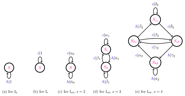
Figure 4: $\epsilon$-Machines describing the stacking of ice I. Nodes represent causal states and are connected by arcs labeled $s|p$, where $s$ is the symbol emitted and $p$ is the probability of making such a transition. (a) The $\epsilon$-machine for ice I_h and (b) ice I_c. Models for disordered stacking sequences of close-packed structures were introduced by Jagodzinski [62, 63]. The model parameter specifying the range of influence between MLs is called the Reichweite $s$. (c) The simplest $\epsilon$-machine in the hc-notation that gives an ice I_sd stacking sequence. (d) The $\epsilon$-machine for $s=3$ ice I_sd and (e) $s=4$ ice I_sd.

Let’s begin with the models used. The $\epsilon$-machines that describe ice I_h and ice I_c are shown in Figs. (4a) and (4b). They are quite similar, both having but one state and one transition each. Computationally, they are quite simple. Also simple is the $\epsilon$-machine shown in Fig. (4c). There are two transitions from a single state, with the probability of a $c$ being $\alpha_{0}$ and an $h$ being $\bar{\alpha}_{0}$. It is apparent that the previous two models are just special cases of this latter one. We recognize that these three models describe independent and identically distributed (IID) stacking processes. They imply no correlations between the symbols. However, the coding scheme used here, the transformation of the $ABC$-notation to the Wyckoff-Jagodzinski notation, builds in stacking constraints and effectively gives a two-ML influence distance. We identify this range of influence as the Reichweite $s$.

The next model commonly used is Jagodzinski’s $s=3$ disorder model in Fig. (4d). Here, the next symbol in the sequence depends only on the previous symbol (either $h$ or $c$), making this a first-order Markov model. The last model explored in the literature is Jagodzinski’s $s=4$ disorder model, and this is depicted in Fig. (4e). Now, the probability of observing the next symbol depends on the previous two symbols, we recognize this as a second-order Markov model. Again, the mapping of the $ABC$-notation to the Wyckoff-Jagodzinski notation folds in an extra two-ML range of influence in terms of the physical stacking of MLs. It is apparent that one could continue this process, considering ever larger Reichweite, i.e., higher-order Markov models, indefinitely. However, finite-range Markov processes are only a small fraction of the possible finite-state processes that one could consider. By finite-state, we mean that there are a finite number of states; but this does not mean that the range of influence need be finite. Simulations of simple solid-state transformations in ZnS (also a close-packed structure) from the hexagonal stacking structure to the cubic one produced stacking processes with an infinite range of influence [27]. Thus, we are led to suspect that despite the excellent agreement between experimental and theoretical diffraction patterns reported by some researchers for ice I, the real process may belong to a computationally more sophisticated class. Chaotic crystallography, with its emphasis on information- and computation-theoretic measures, allows one to recognize the possibility and indeed to ask the relevant questions.

How can we observe or deduce the presence of such sophisticated stacking processes? One way is improved inference techniques. While chaotic crystallography has an inference algorithm, $\epsilon$-machine spectral reconstruction theory [26, 25] that detects finite-range processes from diffraction patterns, there is the possibility of extending it to include infinite-order processes. Also, the simulation studies discussed earlier can result in disordered stacking sequences and there are techniques, such as the subtree merging [22] and Bayesian Structure Inference [66] algorithms, that can discover these finite-state but infinite-range processes from sequential data. This suggests that the appropriate level of comparison between theory, simulation, and experiment is not some signal (the diffraction pattern), but rather the stacking process itself, as specified by the $\epsilon$-machine. Chaotic crystallography is a platform for such comparison.

Also, by studying the $\epsilon$-machine’s causal architecture, i.e., the arrangement of causal states and the transitions connecting them, it is possible to discover the kinds of faults present. Indeed, this was done for ZnS polytypes [26, 28]. Recently, several different kinds of faults where proposed for ice I [57], and a proper analysis of the associated $\epsilon$-machine, combined with theoretical and experimental studies, can elucidate which faults are important in a particular specimen. This could be quite valuable, as there are many possible routes of formation for disordered ice specimens, and different mechanisms, such as solid-state transformations versus growth, likely leave a discernible fingerprint in the causal architecture.

4.2.2 Organization of Aromaticity

Benzene is famous for it’s curious “aromatic” character that stems directly from the six $\pi$ electrons shared between its six carbon atoms and hovering above and below the plane of its carbon-atom ring. To understand this character, chemists are trying to localize the delocalized $\pi$ electrons, partly to understand benzene’s physical character and partly to find new ways to control chemical reactivity and discover new synthetic paths. One goal is to engineer benzene’s novel electronic motif to act as a controllable reaction catalyst. There is an active research program to modify benzene’s aromatic properties by adding on “bicyclic” rings outside the main ring. This led to the creation of tris(bicyclo[2.1.1]hexeno)benzene (TBHB). TBHB’s structure is critical to understanding how to localize benzene’s $\pi$ electrons [67].

Figure 5: (left) Molecular structure of TBHB. Black spheres represent carbon atoms while the white are hydrogen atoms. (right) The so-called “skeletal formula” representation of TBHB. Adapted from Michels-Clark et al.[68], used with permission.

We recount recent experimental probes of TBHB’s structure, demonstrating how an information-theoretic analysis yields additional insight. TBHB is a largely planar molecule that has attracted attention as one of the first confirmed mononuclear benzenoid hydrocarbons with a cyclohexatriene-like geometry [69]. Figure 5 (left) shows the molecular structure of TBHB, and Fig. 5 (right) gives a schematic formula representation. Of particular interest is the central benzene ring, where the internal angles of the carbon-carbon bonds are all 120^∘, but there is remarkable alteration of the two inequivalent bond lengths between the carbons (1.438(5) - 1.349(6) Å)[69]. Of additional interest is the crystallographic structure of TBHB. Here, two crystal morphologies are observed, monoclinic and hexagonal[70]. For this latter structure, X-ray diffraction studies reveal significant diffuse scattering along rods in reciprocal space, a hallmark of planar disorder. Figure 6 (left) shows the positions of the diffuse rods in reciprocal space, and Fig. 6 (right) gives an illustration of the average layer structure of TBHB. We will call the extension of this configuration into a two-dimensional periodic array a ML for TBHB.

Of more recent interest [71, 68], and the problem that concerns us here, is quantifying and describing the disordered stacking structures observed in TBHB. In order to do this, we must specify the possible ML-ML stacking arrangements and establish a convenient nomenclature to express extended stacking structures. The stacking rules and conventions for layers of TBHB can be summarized as follows: (i) While there are three ways that two MLs can be stacked, they are geometrically equivalent and are related by a rotation of 120^∘ about the stacking direction. Thus, there is only single kind of ML-ML relationship. (ii) For triplets of MLs, there are two geometrically inequivalent stacking arrangements. For the case where a molecule in the $(i+2)^{\mathrm{th}}$ ML is directly above one in the $i^{\mathrm{th}}$ ML, this arrangement is called eclipsed. The other distinct possibility is that the $(i+2)^{\mathrm{th}}$ ML occupies one of the other two positions. These are geometrically equivalent, being related by a mirror operation, and are called bent. However, as one advances along the stacking direction, these latter two can be differentiated as rotating in either a clockwise or an anticlockwise fashion. Together, then, we need to distinguish between three different triplets of stacking sequences: an eclipsed triplet, which we symbolize by $e$, a clockwise bent triplet which we will symbolize by $l$, and an anticlockwise bent triplet, symbolized by $r$. We collect these possibilities into the set $\mathcal{A}=\{r,l,e\}$.

Let us imagine a sliding window that permits observation of but three MLs at a time. That three-ML sequence is then assigned a symbol from $\mathcal{A}$. The window then increments along the stacking direction by one ML, so that the last ML in the sequence becomes hidden, and a new ML is revealed. This new three-ML sequence can again be specified by one of the symbols in $\mathcal{A}$, such that the four-ML sequence is given by a two-letter sequence from $\mathcal{A}$. Thus, a physical stacking sequence can be written as sequence over the set of these triplets, $\mathcal{A}=\{r,l,e\}$.

Recently, Michels-Clark et al. [68] compared three different methods of determining stacking structure for disordered TBHB from diffraction patterns: differential evolution, particle swarm optimization, and a genetic algorithm. Although computationally intensive, they find excellent agreement between calculated and reference diffraction patterns, obtaining an $R$-factor fitness of $\overline{R}=0.0077(3)$ for their best case differential evolution algorithm. We analyze that case in detail now.

Michels-Clark et al. [68] assume a second-order Markov process in the $rle$-notation, so that the probabilities of successive symbols are dependent on only the two previous symbols seen, i.e., $\mathcal{A}^{2}=\{rr,rl,re,lr,ll,le,er,el,ee\}$, which they call structural motifs. Michels-Clark et al. [68] directly report that the probability seeing $e$ following a pair of $e$’s as $e_{2}=\Pr(e|ee)=0.008$, which is only two standard deviations above 0. In addition, the probability of the $ee$ sequence itself is only 0.00033. Thus, we neglect the $ee$ sequence when we construct the hidden Markov model and take the remaining eight two-symbol histories as our set of causal states: $\{\mathcal{S}_{rr},\mathcal{S}_{rl},\mathcal{S}_{re},\mathcal{S}_{lr},\mathcal{S}_{ll},\mathcal{S}_{le},\mathcal{S}_{er},\mathcal{S}_{el}\}$. Table 1 of Michels-Clark et al. [68] relates transition probabilities between structural motifs to model parameters, so that we can directly calculate transition parameters from any solution of model parameters. Taking the values for the best case differential evolution solution given in their Table 2, we calculate these probabilities. The resulting $\epsilon$-machine is shown in Fig. 7. In this way, we can give a chaotic crystallographic interpretation of that stacking process.

Figure 6: (left) Schematic illustration of the reciprocal space plane $hk0$. Circles represent the positions of the diffuse scattering ($h-k\neq 3n$) and crosses the positions of the Bragg-like reflections ($h-k=3n$). (right) Average layer structure for TBHB with the layer symmetry being $p(\overline{6})2m$. A two-dimensional array of TBHB molecules thus arranged is called a modular layer (ML). Adapted from Bürgi et al.[71], used with permission.

With their relatively large asymptotic state probabilities (0.23) and their large inter-state transition probabilities (0.97), there is one causal state cycle [26, 25] that dominates the $\epsilon$-machine: [$\mathcal{S}_{rr}\mathcal{S}_{rl}\mathcal{S}_{ll}\mathcal{S}_{lr}$]. This causal state cycle gives rise to the observed parent structure ($rrll$)^∗. There are two kinds of deviations from this structure: (i) those that weakly connect the four causal states of this dominant causal state cycle, intra-causal state state faults, and (ii) those that break out of the dominant causal state cycle and visit peripheral causal states, inter-causal state faults.

Of the first kind, one can think of two cases, the insertion of a symbol or the deletion of a symbol into the normal stacking sequence. The self-state transition loops on $\mathcal{S}_{ll}$ and $\mathcal{S}_{rr}$ have the effect of inserting an extra modular layer:

$$\dots l\,l\,r\,r\,l\,l\,{\underline{l}}\,r\,r\,l\,l\,\dots,$$

or

$$\dots l\,l\,r\,r\,l\,l\,r\,r\,{\underline{r}}\,l\,l\,\dots,$$

where the inserted symbol as observed by scanning from the left is underlined. Conversely, the two transitions $\mathcal{S}_{lr}\to\mathcal{S}_{rl}$ and $\mathcal{S}_{rl}\to\mathcal{S}_{lr}$ have the effect of deleting a symbol, i.e.:

$$\dots l\,l\,r\,r\,l\,l\,r\,|\,l\,l\,\dots,$$

or

$$\dots l\,l\,r\,r\,l\,|\,r\,r\,l\,l\,\dots,$$

where the pike ‘$|$’ indicates the position of the deleted symbol as the sequence is scanned from the left. Faulting structures of this kind are often referred to as extrinsic (insertion of a symbol) and intrinsic (deletion of a symbol), respectively. For the specimen analyzed here, there is a probability of 0.01 that one of these faults will occur in dominant causal state cycle [$\mathcal{S}_{rr}\mathcal{S}_{rl}\mathcal{S}_{ll}\mathcal{S}_{lr}$] as each causal state is visited.

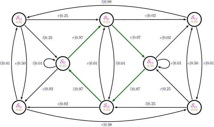
Figure 7: TBHB causal-state architecture. The alphabet is $\mathcal{A}=\{l,r,e\}$. In this nomenclature, the process is second-order Markovian and, thus, causal states are specified by the last two symbols observed. The causal states are labeled with their asymptotic state probabilities. There is one closed cycle that dominates the graph, and that is the four-state loop [$\mathcal{S}_{rr}\mathcal{S}_{rl}\mathcal{S}_{ll}\mathcal{S}_{lr}$] (green transition arcs). That this nearly periodic sequence is so well represented suggests that this structure is nearly crystalline, i.e. periodic, but does have faults.

A second kind of fault breaks out of this dominant causal state cycle on emission of an $e$. There is a 0.02 probability of this happening at each causal state in the dominant causal state cycle. Generically, these transitions are given by $\mathcal{S}_{yz}\to\mathcal{S}_{ze}$, where $y,z\in\{l,r\}$. Then, one almost always (0.98 probability) observes that the symbol following $e$ is opposite the one that preceded the $e$, i.e.:

$$\mathcal{S}_{xr}\to\mathcal{S}_{re}\to\mathcal{S}_{el}\,\,\,\,{\mathrm{or}}$$

$$\mathcal{S}_{xl}\to\mathcal{S}_{le}\to\mathcal{S}_{er}~{}.$$

In other words, an $e$ is almost always sandwiched between two unlike symbols drawn from $l$ and $r$. There is a 0.50 probability that the sequence will return to the dominant causal state cycle at this point on emission of either a $l$ or $r$. If not, then another $e$ is observed. Thus, even though pairs of $e$’s ($ee$) are unlikely (and, in fact, prohibited in this $\epsilon$-machine) the probability of observing two $e$’s separated by a single $r$ or $l$ is surprisingly large. It appears that they may ‘clump’ into small regions.

4.2.3 Towards a Unified View of Material Structure

How does all of this fit together? Let’s contrast the chore of the crystallographer tasked with determining the structure of a periodic material and nonperiodic one. For the full three-dimensional periodic case, there are seven possible crystal systems: triclinic, monoclinic, orthogonal, tetragonal, cubic, trigonal, and hexagonal. One, of course, can be more specific and note that there are 230 crystallographic space groups. A periodic crystal must belong to one and only one of them. Thus, crystallography is equipped with tools that partition the space of all possible crystal structures into a finite number of nonoverlapping sets. Of all the bewildering number ways one might imagine putting atoms together in a periodic three-dimensional array, this limited classification system exhausts the possibilities. One can discuss the similarities between the different systems [72] and otherwise approach a genuine understanding of varieties of possible structures. But can the same be said for nonperiodic materials?

To simplify the discussion, let’s confine our attention to the one-dimensional case of stacking 1000 MLs. Let’s suppose that this is over an alphabet of two. How many possible stacking sequences are there? Well, there are $2^{1000}\approx 10^{301}$. Given that there are about $10^{80}$ protons in the observable universe, it is clear that a comprehensive listing is simply not possible. And if it were, it is questionable how helpful it would be. For these disordered materials, then, we are forced to appeal to statistical methods. Instead of a classification scheme fine-grained at the level of individual sequences, we instead collect all sequences that have the same statistical properties into a set. Colloquially, each set is represents a stacking process. Operationally, we attempt to identify to which process a particular sequence belongs, and then we analyze the process in lieu of the particular sequence.

Each of the graphs in Fig. 4 and Fig. 7 specifies a particular process and defines a hidden Markov model. While there are still an infinite number of possible processes in the limit of indefinitely long sequences, a kind of order has been imposed. We can, for example, enumerate all the processes over a two-symbol alphabet with just one state. There is but one, and it is shown in Fig. 4c. (Figs. 4a,b are just special cases of Fig. 4c.) For two-state binary processes, there are thirteen [66]. For binary processes, the number of distinct processes up to six states has been tabulated [73]. Thus, chaotic crystallography does for disordered materials much the same service that classical crystallography does for perfectly ordered ones: it organizes and structures the space of possible atomic arrangements. Further, it allows comparison of the hidden Markov models between different materials in much the same way that crystal structures of different materials are compared according to which, for example, crystal system they belong.

We contend then that the hidden Markov models describing not only different specimens of the same material, but different materials altogether can be compared, either by direct examination of the graphical model of the process or by information measures that characterize various computational requirements. As an example, we can compare measures of intrinsic computation between the two materials considered in the previous subsections as well as that of a third layered material, ZnS. Of the many measures one can select, we choose to examine these materials’ informational organization via a complexity-entropy diagram [23]. A complexity-entropy diagram plots, for each stacking process, the entropy rate ${h_{\mu}}$ of a symbol sequence discussed in Section § 3 and the mutual information between two halves of the specimen, the excess entropy ${\bf E}$, introduced in Sec. § 4. These measures can be calculated directly from the hidden Markov model for the stacking processes.

We begin with ice. Note that ice I_c and ice I_h are both described by single-state machines and, thus, each half of the crystal shares no information with the other half, giving ${\bf E}({\rm{I}_{c}})={\bf E}({\rm{I}_{h}})=0$ bits. Similarly, being perfectly ordered, we find ${h_{\mu}}({\rm{I}_{c}})={h_{\mu}}({\rm{I}_{h}})=0$ bits/ML. For ice I_sd, we calculate this quantity for a number of experimental specimens reported in the literature. Malkin et al. [52] performed X-ray diffraction studies of several samples of ice I that has been recrystallized from ice II and heated at rates between 0.1 to 30 K per minute over temperature ranges of 148 - 168 K. They use the $s=4$ Jagodzinski disorder model to analyze their results, and we find by direct calculation from the data given in their Table 4 that these information measures cluster in the range of ${\bf E}({\rm{I}_{sd}})\approx 0.10-0.15$ bits and ${h_{\mu}}({\rm{I}_{sd}})\approx 0.75-0.90$ bits/ML. Murray et al. [58] carried out similar studies on ice I deposited as amorphous ice from the vapor phase onto a glass substrate at 110 K. The sample was subsequently warmed at a rate of 1 K per minute, and they report diffraction patterns recorded at selected temperatures in the range of 125 - 160 K. They too analyzed the diffraction patterns using the $s=4$ Jagodzinski disorder model, although they found that memory effects were negligible. We find by direct calculation from the data given in their Table 1 that these information measures cluster near ${\bf E}({\rm{I}_{sd}})\approx 0$ bits and ${h_{\mu}}({\rm{I}_{sd}})\approx 0.95-1.00$ bits/ML. We can do the same for TBHB. We find ${\bf E}({\rm{TBHB}})=1.9$ bits and ${h_{\mu}}({\rm{TBHB}})=0.27$ bits/ML. For comparison, we also consider these quantities for several specimens of ZnS analyzed elsewhere [28]. Lastly, to contrast with these disordered samples, we consider a one-dimensional process that has characteristics similar to those of a quasicrystal, the Thue-Morse Process (TM) [74]. Like a quasicrystal, it is completely ‘ordered’, but nonperiodic. We have $\lim_{N\to\infty}{\bf E}({\rm{TM}})=\infty$ bits, where $N$ is the number of layers in the specimen, and ${h_{\mu}}({\rm{TM}})=0$ bits/ML.

Since the maximum possible stacking disorder is 1 bit/ML for ice I, we can see that disordered ice I really is, well, disordered. Additionally, very little information (${\bf E}$) is shared between the different halves. There is little one can predict about one half of the specimen knowing the other half. The clustering of the these information measures does lend credibility to the notion that ice I_sd is a ‘new’ form of ice. We would, however, exercise caution in referring to this as a distinct thermodynamic phase of ice. Observe that it is not only not well defined in stacking-sequence space, i.e. there are many sequences that correspond to ice I_sd, but we also see from the spread of information measures on the complexity-entropy diagram, it is not well defined in process-space either. We prefer the interpretation that these specimens are chaotic crystals, each being described by a different hidden Markov model and each exhibiting different measures of information processing. Thus, they really do not constitute a separate phase in the same sense that ice I_c and ice I_h are. Ice I_sd is, at least at the moment, an umbrella term for ice I with a largely randomly stacking of hexagonal and cubic layers. We do note that information-theoretic measures can distinguish between ice I_sd samples having different histories of under different thermodynamic conditions.

In contrast to the near complete disorder of these ice I_sd specimens, the TBHB sample appears to be much more organized. Not only is more information shared between the two halves, but the entropy rate is much less. Indeed, as noted before, there is a prominent cycle on the graph of Fig. 7 that is nearly periodic. ZnS presents an intermediate case. Its specimens are similar to ice I in that they are either grown disordered or caught in the transformation between crystalline phases: a hexagonal phase and a cubic one. Generically, however, ZnS appears to have more structured intermediate states, suggesting a more structured transformation, likely as a result of significant constraints on the types disordering mechanisms in play. We can speculate that though ice I and ZnS can both be described as close-packed structures, the disordering and transformation mechanisms are at least quantitatively, if not qualitatively, different for each.

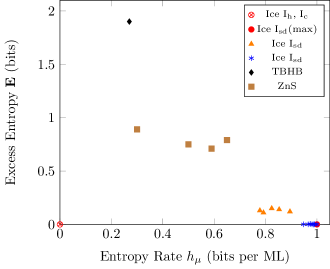
Figure 8: The variety of intrinsic computation as revealed by a complexity-entropy diagram. For disordered ice, we plot values calculated from experiments on I_sd ( $\ast$ from Table 1 of ref [58] and $\blacktriangle$ from Table 4 of ref [52]); TBHB ($\blacklozenge$ from ref [68]); and ZnS ( $\blacksquare$ from ref [28]). For reference, we plot the complexity-entropy point for both I_h and I_c ( $\otimes$) as well as I_sd ( ●). Not shown is the point for the TM process (see text), a one-dimensional surrogate for a quasicrystal. We would find it indefinitely high on the vertical axis (the excess entropy is divergent with a vanishing small entropy rate for large specimens). Different values of intrinsic computation indicate significant differences in the organization of the stacking process for each material as well as their entropy densities.

Examining Fig. 8, we see that the complexity-entropy diagram also provides a partitioning for the kinds of structures that can can exist. For example, any periodic process has zero entropy, thus on a complexity-entropy diagram all perfect crystals are confined to the vertical axis. This, then, makes concrete just how special crystallinity is. Similarly, quasicrystals inhabit the upper left corner of the diagram, also confined to the vertical axis. Thus, while quite interesting, quasicrystals are informationally rather special organizations. All the space to the right of the vertical axis is occupied by entropic crystals—just the kinds of specimen that chaotic crystallography is ideally suited to describe. Thus, chaotic crystallography introduces tools to quantify these structures and represents a significant expansion over the domain of classical crystallography.

Although we maintain that understanding structure in itself is a worthy enough goal, we are mindful that one of the fruits to be harvested from this inquiry is the possible exploitation of the connection between structure and function. The interrelationship between structure and material properties is quite well known. Carbon can exist as face-centered cubic crystal and, when a specimen is so ordered, we call it a diamond. More commonly, carbon is found in hexagonal sheets and is known as graphite. Carbon can also be arranged as nanotubes and spherical shells informally called Bucky balls. And, though each of these is equivalent by composition, their material properties are vastly different. Structure matters. Less drastically, different kinds of stacking structures change material properties in more subtle ways. Brafman and Steinberger [76] noticed that by changing from one kind of periodic stacking structure in ZnS to another, the degree of birefringence changes. Indeed, this change appeared to depend on only a single parameter, the hexagonality, which is the fraction of layers hexagonally related to their neighbors, given by $\Pr(h)$. And, perhaps consequentially, it did so in a very smooth and predictable way. We know that stacking structure affects other material properties, such as the diffraction pattern and, clearly, the correlation functions. It requires little imagination to speculate that other properties may be similarly affected.

Let us then return to the case of stacking $1000$ MLs. Suppose we task a materials scientist to investigate the possible material properties obtainable from different stacking sequences. Even in the simple binary case, as we saw above, there are approximately $10^{301}$ such sequences. Thus, (the admittedly naive approach of) a detailed sequence-by-sequence analysis is unfeasible—either experimentally, theoretically, or via simulation. Yet absent any theory of disorder in materials, such a brute force investigative approach might be thought necessary. A chaotic crystallography perspective immediately equips the materials scientist with tools to approach the problem. She knows, for instance, that many materials properties are dictated by and calculable from knowledge of the stacking process alone. Thus, instead of trying to tackle the problem sequence-by-sequence, it is profitable instead to approach it process-by-process. Although the space is still enormous, it is considerably smaller and, importantly, is now systematized. Starting with simple processes and proceeding to more complex ones, might, for example, be an effective strategy. Furthermore, properties may not even depend on the stacking process details, but may instead correlate with overall statistical properties or information theoretic measures. The case of the birefringence of ZnS hints at this. A single statistical parameter correlates with the observed birefringence; at least for periodic stacking sequences. Also, the diffraction pattern is known to depend only on the pairwise correlations between MLs. It is well known that different stacking processes can have the same correlation functions, suggesting that an even less fine-grained approach may be profitable. To the extent that transmission properties through disordered potentials depend only on correlation functions [41], here too a less fine-grained approach may be useful.

One may object and question whether we are guaranteed that all material properties are the same for all realizations of a process. We are not. However, theoretical results suggesting the important parameters to consider, coupled with experimental observations and the outcomes of simulations, can give confidence that a particular property under study is an ensemble property. Unquestionably, much of the connection between information-theoretic properties and materials properties remains unexplored. Along the lines presented here and paralleling Schrödinger’s principled, but speculative thoughts about life’s organization, the abundant hints of intimate connections are too promising and possible rewards of finding and exploiting such connections are too rich to not explore.

We note too that the exercise of predicting material properties from structure is by no means academic: The Materials Genome Project [77] is a coordinated and dedicated effort spanning theoretical, experimental, and simulation studies attempting to do just this. Given the sheer variety of possible arrangements of atoms, an organizational scheme that structures the space of possibilities is an absolute necessity. Otherwise, researchers will find themselves relying on intuition—formidable certainly, but all too often unreliable—alone to propose and assemble possible configurations with novel material properties. Without too much exaggeration, it is a akin to banging on a keyboard hoping to finger out one of Shakespeare’s sonnets: Possible yes, but ever so much more likely if one knows the rules of English grammar.

5 Thermodynamics of Material Computation

Up to this point, we focused exclusively on informational properties embedded in the static structure of “chaotic” materials, ignoring temporal dynamics … of their growth, their functional behavior in the “wild”, and the like. A full story, though, requires a thermodynamic accounting of the informational aspects of such materials—the energetics of their equilibrium and nonequilibrium configurations, the energetics of how they come to be, how they are transformed, and what functions they support. Here, to illustrate the connections between intrinsic information and energetic costs, we briefly review recent explorations of Maxwell’s Demon and a ratchet model that describes how molecular “engines” can store and process information as they traverse a control sequence.

5.1 Szilard’s Single-Molecule Engine

Biological macromolecules [78, 79, 80] perform tasks that involve the simultaneous manipulation of energy, information, and matter. Though we can sometimes identify such functioning—in the current gating of a membrane ion channel [81, 82] that supports propagating spike trains along a neuronal axon or in a motor protein hauling nutrients across a cell’s microtubule highways [78]—it is not well understood. Understanding calls on a thermodynamics of nanoscale systems that operate far out of equilibrium and on a physics of information that quantitatively identifies organization and function. At root, we must rectify this functioning with the entropy generation dictated by the Second Law of Thermodynamics. James Clerk Maxwell introduced the Demon that now bears his name to highlight the essential paradox. If a Demon can measure the state of a molecular system and take actions based on that knowledge, the Second Law can be violated: sorting slow and fast molecules onto separate sides of a partition creates a temperature gradient that a heat engine can convert to useful work. In this way, Demon “intelligence”—or, in our vocabulary, information processing—can convert thermal fluctuations (disorganized energy) to work (organized energy).

In 1929 Leo Szilard introduced an ideal Maxwellian Demon for examining the role of information processing in the Second Law [83]; a thought experiment that a decade or so later provided an impetus to Shannon’s communication theory [84]. Szilard’s Engine consists of three components: a controller (the Demon), a thermodynamic system (a molecule in a box), and a heat reservoir that keeps both thermalized to a temperature $T$. It operates by a simple mechanism of a repeating three-step cycle of measurement, control, and erasure. During measurement, a barrier is inserted midway in the box, constraining the molecule either to box’s left or right half, and the Demon memory changes to reflect on which side the molecule is. In the thermodynamic control step, the Demon uses that knowledge to allow the molecule to push the barrier to the side opposite the molecule, extracting $\int P~{}dV=k_{\text{B}}T\ln 2$ work from the thermal reservoir. In the erasure step, the Demon resets its finite memory to a default state, so that it can perform measurement again. The periodic protocol cycle of measurement, control, and erasure repeats endlessly and deterministically. The net result being the extraction of work from the reservoir balanced by entropy created by changes in the Demon’s memory. The Second Law is respected and the Demon exorcised, since dumping that entropy to the heat bath requires a work flow that exactly compensates energy gained during the control step.

Connecting nonlinear dynamics to the thermodynamics of Szilard’s Engine, we recently showed that its measurement-control-erasure barrier-sliding protocol is equivalent to a discrete-time two-dimensional map from unit square to itself [85]. This explicit construction establishes that Szilard’s Engine is a chaotic system whose component maps are thermodynamic transformations—what we now call a piecewise thermodynamical system. An animation of the Szilard Engine, recast as this chaotic dynamical system, can be viewed at http://csc.ucdavis.edu/~cmg/compmech/pubs/dds.htm.

What does chaos in the Szilard Engine mean? The joint system generates information—information that the Demon must keep repeatedly measuring to stay synchronized to the molecule’s position. On the one hand, information is generated by the heat reservoir through state-space expansion during control. This is the chaotic instability in the Engine when viewed as a dynamical system. And, on the other, information is stored by the Demon (temporarily) so that it can extract energy from the reservoir by allowing the partition to move in the appropriate direction. To return the Engine to the same initial state, that stored information must be erased. This dynamically contracts state-space and so is locally dissipative, giving up energy to the reservoir.

The overall information production rate is given by the Engine’s Kolmogorov-Sinai entropy ${h_{\mu}}$ [86]. This measures the flow of information from the molecular subsystem into the Demon: information harvested from the reservoir and used by the Demon to convert thermal energy into work. Simply stated, the degree of chaos determines the rate of energy extraction from the reservoir. Moreover, in its basic configuration with the barrier placed in the box’s middle and its memory states being of equal size, the Demon’s molecule-position measurements are optimal. It uses all of the information generated ${h_{\mu}}$ by the thermodynamic system: All of the generated information ${h_{\mu}}$ is bound information ${b_{\mu}}$; none of the generated information is lost (${r_{\mu}}$ vanishes).

Critically, the dynamical Szilard Engine shows that a widely held belief about the thermodynamic costs of information processing—the so-called Landauer Principle [87, 88, 89, 90, 91]: each erased bit costs $k_{\text{B}}T\ln 2$ of dissipated energy and the act of measurement comes at no thermodynamic cost—is at best a special case [92, 93, 94, 85]. As the partition location varies and the Demon memory cells change size, both measurement and erasure can dissipate any positive or negative amount of heat. Specifically, there are Szilard Engine configurations that directly violate Landauer’s Principle: erasure is thermodynamically free and measurement is costly—an anti-Landauer Principle. The result is that the Szilard Engine achieves a lower bound on energy dissipation expressed as the sum of measurement and erasure thermodynamic costs. In this, the Szilard Engine captures an optimality in the conversion of information into work that is analogous to a Carnot Engine’s optimal efficiency when converting a difference in thermal energies to work.

5.2 Information Catalysts

Szilard’s Engine is one of the simplest controlled thermodynamic devices that lays bare the tension between the Second Law and functionality of an information-gathering entity or subsystem (the Demon). The net work extracted exactly balances the thermodynamic (entropic) costs. This was Szilard’s main point, though we see that his Engine was not very functional, merely consistent with the Second Law. The major contribution was that, long before Shannon’s information theory, Szilard recognized the importance of the Demon’s information acquisition and storage in resolving Maxwell’s paradox.

This allows us to move to a more sophisticated device that uses a reservoir of information (a string of random bits) to extract net positive work from a heat reservoir. To set the stage for the thermodynamics we are interested in, but staying in the spirit of complex materials, let’s re-imagine the Szilard Engine implemented as an enzyme macromolecule whose conformational states implement the measurement-control-erase protocol. Moreover, let this enzyme traverse a one-dimensional periodic crystal—say, a strand of DNA—reading its successive base-pairs to obtain individual Measurement, Control, Erase protocol commands. The preceding thermodynamics and informational analysis thus apply to such a molecular engine—an actively controlled system that can rectify fluctuations, being only temporarily, locally inconsistent with the Second Law.

Let’s go one step further, though, to imagine a functional enzyme that over a thermodynamic cycle extracts net positive work from an information reservoir to store or release energy as it assembles or disassembles a chain of small molecular components. In this, we replace the one-dimensional ”control” molecule with a set of random bits that come into local equilibrium with the enzyme. As they do, the enzyme’s dynamic shifts to catalyze assembling the components. The shift allows the enzyme to selectively use energy from a reservoir, say an ATP-rich environment whose molecules the machine accesses when energy is needed (ATP $\to$ ADP) or given up (ADP $\to$ ATP). Figure 9 illustrates the new, functional molecular machine.

In this way, the imagined enzyme acts as an information catalyst that facilitates, via what are otherwise thermodynamically unfavorable reactions, the assembly of the chain of molecular components. In the 1940s, Leon Brillouin [95] and Norbert Wiener [96], early pioneers in the physics of information, viewed enzymes as just these kinds of catalysts. In particular, Brillouin proposed a rather similar “negative catalysis” as the molecular substrate that generated negentropy—the ordering principle Schrodinger identified as necessary to sustain life processes consistent with the Second Law. Only much later would such “information molecules” be championed by the evolutionary biologists John Maynard Smith and Eors Szathmary [97].

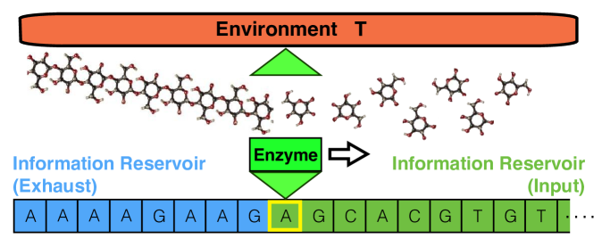
Figure 9: Information catalyst: An enzymatic molecular Maxwellian Demon thermalizes with a succession of random bits (information reservoir), each changing its catalytic activity to overcome energy barriers to assemble a chain of simple molecular components. The environment, at constant temperature $T$, provides energy-rich molecules needed to drive the catalyzed reactions and the chain component molecules. (Cf. the information ratchet of Ref. [98].)

We recently analyzed the thermodynamics of a class of memoryful information catalysts [98] for which all correlations among system components could be explicitly accounted. This gave an exact, analytical treatment of the thermodynamically relevant Shannon information change from the input information reservoir (bit string with entropy rate ${h_{\mu}}$) to an exhaust reservoir (bit string with entropy rate ${h_{\mu}}^{\prime}$). The result was a refined and broadly applicable Second Law that properly accounts for the intrinsic information processing reflected in the accumulation of temporal correlations. On the one hand, the result gives an informational upper bound on the maximum average work $\langle W\rangle$ extracted per cycle:

$$\langle W\rangle \leq k_{\text{B}}T\ln 2\,({h_{\mu}}^{\prime}-{h_{\mu}})~{},$$

where $k_{\text{B}}$ is Boltzmann’s constant and $T$ is the environment’s temperature. On the other hand, this new Second Law bounds the energy needed to materially drive transforming the input information to the output information. That is, it upper bounds the amount $-\langle W\rangle$ of input work to a physical system to support a given rate of intrinsic computation, interpreted as producing a more ordered output—a reduction in entropy rate.

This Second Law allows us to identify the Demon’s thermodynamic functions. Depending on model parameters, it acts as an engine, extracting energy from a single reservoir and converting it into work ($\langle W\rangle>0$) by randomizing the input information (${h_{\mu}}^{\prime}-{h_{\mu}}>0$), or as an information eraser, erasing information (${h_{\mu}}^{\prime}-{h_{\mu}}<0$) in the input at the cost of the external input of work ($\langle W\rangle<0$). Moreover, the Demon supports a counterintuitive functionality. In contrast to previous erasers that only decreased single-bit uncertainty $\operatorname{H}[X_{0}]$, it sports a new kind of eraser that removes multiple-bit uncertainties by adding correlation (temporal order), while single-bit uncertainties are actually increased ($\operatorname{H}^{\prime}[X_{0}]-\operatorname{H}[X_{0}]>0$). This modality leads to a provocative interpretation of life processes: The existence of natural Demons with memory (internal states) is a sign that they have been adapted to leverage temporally correlated fluctuations in their environment.

6 Conclusions

We have come a long way from Schrödinger’s prescient insight on aperiodic crystals. We argued, across several rather different scales of space and time and several distinct application domains, that there is an intimate link between the physics of life and understanding the informational basis of biological processes when viewed in terms of life’s constituent complex materials. We noted, along the way, the close connection between new experimental techniques and novel theoretical foundations—a connection necessary for advancing our understanding of biological organization and processes. We argued for the importance of structure and strove to show that we can now directly and quantitatively talk about organization in disordered materials, a consequence of breaking away from viewing crystals as only periodic [99, 44]. These structured-disordered materials, in their ability to store and process information, presumably played a role in the transition from mere molecules to material organizations that became substrates supporting biology [100]. For biology, of course, its noncrystalline “disorder” is much much more, it encodes the information necessary for life. Thus, biological matter is more than wet, squishy “soft matter”; it is informational matter. DNA, RNA, and proteins are molecules of information [97, 95, 96]. So much so that DNA, for example, can be programmed [101, 102, 103]. And, in a complementary way, the parallels driving our development here perhaps give an alternative view of “material genomics” [77].

What distinguishes biological matter from mere physical matter is that the information in the former encodes organization and that organization takes on catalytic function through interactions in a structurally diverse environment. Moreover and critically, these characters are expressed in a way that leads to increasingly novel, complex chemical structures—structures that form into entities with differential replication rates [104]. And the high-replication entities, in turn, modify the environment, building “niches” that enhance replication; completing a thermodynamic cycle, whose long-term evolutionary dynamics are thought to be creatively open-ended.

We saw that pondering Schrödinger’s view of the physical basis of life raised questions of order, disorder, and structure in one-dimensional materials. Chaotic crystallography emerged as an overarching theory for the organization of close-packed materials. It gave a consistent way to describe, at one and the same time, order and disorder in layer stacking in ice and aromatic compounds and, generally, in one-dimensional chaotic crystals. And, in this, it hints at a role that local (dis)ordering can play in enhancing how biomolecules function synergistically in solution. The issue of biological function forced us to probe more deeply into its consistency with the Second Law of Thermodynamics. We then turned to consider two simple cases of Maxwellian molecular Demons to illustrate that the Second Law of Thermodynamics is perfectly consistent with the informational character and functionality of smart molecules—that thermodynamics can begin to describe the energetics of such information catalysts.

Admittedly, we addressed only in a cursory way several major challenges an informational view of matter poses. Shannon introduced information as surprise and we showed that this readily led to seeing how information is stored, created, and transmitted. We only just broached the abiding question, however, of how these kinds of information contribute to material functionality. Szilard’s Engine and related information catalysts hinted at how we will come to analyze functional information in complex materials and biomolecules. Hopefully, the informational perspective will be sufficiently fruitful to extend to analyzing how such structured objects function in their environments—how, for example, water plays a critical role in biomolecular interactions and function.

The authors thank Alec Boyd, Korana Burke, Ryan James, Xincheng Lei, Dibyendu Mandal, and John Mahoney for helpful conversations. We thank the Santa Fe Institute for its hospitality during visits. JPC is an SFI External Faculty member.

This material is based upon work supported by, or in part by, the U S. Army Research Laboratory and the U. S. Army Research Office under contract W911NF-13-1-0390.

We have no competing interests.

JPC and DPV wrote the manuscript jointly.

References

- [1] Kinne-Saffran E & Kinne RKH 1999. Vitalism and synthesis of urea. Am. J. Nephrol, 19, 290–294.
- [2] Wilson EO 1998. Consilience: The Unity of Knowledge. Alfred A. Knopf.
- [3] Watson JD & Crick FHC 1953. A structure for deoxyribose nucleic acid. Nature, 171, 737–738.
- [4] Fraser CM et al. 1995. The minimal gene complement of Mycoplasma genitalium. Science, 270, 397–404.
- [5] Shannon CE 1948. The mathematical theory of communication. Bell Sys. Tech. J., 27, 379–423; 623–656.
- [6] Cover TM & Thomas JA 2006. Elements of Information Theory. Wiley-Interscience, 2 edn.
- [7] Schrödinger E 1992. What is Life?. Cambridge University Press.
- [8] Gleick J 2011. The Information: A History, A Theory, A Flood. Pantheon Books.
- [9] Shannon CE 1956. The bandwagon. IEEE T. Inform. Theory, 2, 3.
- [10] Shechtman D, Blech I, Gratias D & Cahn JW 1984. Metallic phase with long-range orientational order and no translational symmetry. Phys. Rev. Lett., 53, 1951–1953.
- [11] International Union of Crystallography 2015. http://reference.iucr.org/dictionary/Aperiodic_crystal, [online; accessed 14-Jun-2015].
- [12] Baake M & Grimm U 2013. Aperiodic Order: Volume 1, A Mathematical Invitation. Encyclopedia of Mathematics and its Applications (Book 149), Cambridge University Press.
- [13] James RG, Ellison CJ & Crutchfield JP 2011. Anatomy of a bit: Information in a time series observation. Chaos, 21, 037109.
- [14] James RG, Burke K & Crutchfield JP 2014. Chaos forgets and remembers: Measuring information creation, destruction, and storage. Phys. Lett. A, 378, 2124 – 2127.
- [15] Ellison CJ, Mahoney JR & Crutchfield JP 2009. Prediction, retrodiction, and the amount of information stored in the present. J. Stat. Phys., 136, 1005–1034.
- [16] Crutchfield JP, Ellison CJ & Mahoney JR 2009. Time’s barbed arrow: Irreversibility, crypticity, and stored information. Phys. Rev. Lett., 103, 094101.
- [17] Mahoney JR, Ellison CJ & Crutchfield JP 2009. Information accessibility and cryptic processes. Journal of Physics A: Mathematical and Theoretical, 42, 362002.
- [18] Mahoney JR, Ellison CJ, James RG & Crutchfield JP 2011. How hidden are hidden processes? A primer on crypticity and entropy convergence. Chaos, 21, 037112.
- [19] Ara PM, James RG & Crutchfield JP 2015. The elusive present: Hidden past and future dependence and why we build models. SFI Working Paper 15-07-024; arxiv.org:1507.00672 [cond-mat.stat-mech].
- [20] Crutchfield JP, Ellison CJ & Riechers PM 2013., Exact complexity: The spectral decomposition of intrinsic computation. Arxiv:1309.3792 [cond-mat.stat-mech]; Santa Fe Institute Working Paper 13-09-028.
- [21] Riechers PM, Varn DP & Crutchfield JP 2015. Pairwise correlations in layered close-packed structures. Acta Crystallogr. A, 71, 423–443.
- [22] Crutchfield JP & Young K 1989. Inferring statistical complexity. Phys. Rev. Lett., 63, 105–108.
- [23] Feldman DP, McTague CS & Crutchfield JP 2008. The organization of intrinsic computation: Complexity-entropy diagrams and the diversity of natural information processing. CHAOS, 18, 043106.
- [24] Crutchfield JP 1994. The calculi of emergence: Computation, dynamics, and induction. Physica D, 75, 11–54.
- [25] Varn DP, Canright GS & Crutchfield JP 2013. -Machine spectral reconstruction theory: A direct method for inferring planar disorder and structure from X-ray diffraction studies. Acta Crystallogr. A, 69, 197–206.
- [26] Varn DP, Canright GS & Crutchfield JP 2002. Discovering planar disorder in close-packed structures from X-ray diffraction: Beyond the fault model. Phys. Rev. B, 66, 174110.
- [27] Varn DP & Crutchfield JP 2004. From finite to infinite range order via annealing: The causal architecture of deformation faulting in annealed close-packed crystals. Phys. Lett. A, 324, 299–307.
- [28] Varn DP, Canright GS & Crutchfield JP 2007. Inferring planar disorder in close-packed structures via -machine spectral reconstruction theory: Structure and intrinsic computation in zinc sulfide. Acta Crystallogr. B, 63, 169–182.
- [29] Varn DP, Canright GS & Crutchfield JP 2013. Inferring planar disorder in close-packed structures via -machine spectral reconstruction theory: Examples from simulated diffraction patterns. Acta Crystallogr. A, 69, 413–426.
- [30] Riechers PM, Varn DP & Crutchfield JP 2014., Diffraction patterns of layered close-packed structures from hidden Markov models. Arxiv.org:1410.5028 [cond.mat]; Santa Fe Institute Working Paper 14-10-38.
- [31] Dornberger-Schiff K 1956. On order-disorder structures (OD-structures). Acta Crystallogr., 9, 593–601.
- [32] Mackay AL 1986. Generalized crystallography. Computers & Mathematics with Applications, B12, 21–37.
- [33] Mackay AL 1995. Generalized crystallography. J. Mol. Struc-THEOCHEM, 336, 293–303.
- [34] Frank FC 1951. The growth of carborundum: Dislocations and polytypism. Philos. Mag., 42, 1014–1021.
- [35] Sebastian MT & Krishna P 1994. Random, Non-Random and Periodic Faulting in Crystals. Gordon and Breach.
- [36] Rempel A & Magerl A 2010. Non-periodicity in nanoparticles with close-packed structures. Acta Crystallogr. A, 66, 479–483.
- [37] Varn DP & Canright GS 2001. The crystal problem for polytypes. Acta Crystallogr. A, 57, 4–19.
- [38] Yeomans J 1988. The theory and application of axial Ising models. Solid State Phys., 41, 151–200.
- [39] Varn DP & Crutchfield JP 2015. Chaotic crystallography: How the physics of information reveals structural order in materials. Curr. Opin. Chem. Eng., 7, 47–56.
- [40] Anderson PW 1958. Absence of diffusion in certain random lattices. Phys. Rev., 109, 1492–1505.
- [41] Izrailev FM, Krokhin AA & Makarov NM 2012. Anomalous localization in low-dimensional systems with correlated disorder. Phys. Rep., 512, 125–254.
- [42] Lei X, Varn DP, Riechers PM & Crutchfield JP 2015. Transmission thru chaotic crystals: An information-theoretic perspective. p. in preparation.
- [43] Wiersma DS 2013. Disordered photonics. Nat. Photonics, 7, 188–196.
- [44] Ball P 2014. Material Witness: Beyond the crystal. Nat. Mater., 13, 1003.
- [45] Leuschner D 1991. Entropic structure measures in one-dimensional (1d) crystallography – A paradigm. Cryst. Res. Technol., 26, 895–900.
- [46] Le Berre M, Ressayre E, Tallet A, Pomeau Y & Di Menza D 2002. Example of a chaotic crystal: The labyrinth. Phys. Rev. E, 66, 026203.
- [47] Ball P 2008. Water as an Active Constituent in Cell Biology. Chem. Rev., 108, 74–108.
- [48] Ball P 2008. Water as a biomolecule. ChemPhysChem., 9, 2677–2685.
- [49] Attard E, Yang H, Delort AM, Amato P, Pöschl U, Glaux C, Koop T & Morris CE 2012. Effects of atmospheric conditions on ice nucleation activity of pseudomonas. Atmos. Chem. Phys., 12, 10667–10677.
- [50] Salzmann CG, Radaelli PG, Slater B & Finney JL 2011. The polymorphism of ice: Five unresolved questions. Phys. Chem. Chem. Phys., 13, 18468–18480.
- [51] Fuentes-Landete V et al. 2015. Crystalline and amorphous ices. Debenedetti PG, Ricci MA & Bruni F (eds.), Proceedings of the International School of Physics “Enrico Fermi" Course 187 “Water: Fundamentals as the Basis for Understanding the Environment and Promoting Technology", IOS.
- [52] Malkin TL, Murray BJ & Salzmann CG 2015. Stacking disorder in ice I. Phys. Chem. Chem. Phys., 60, 60–76.
- [53] Thürmer K & Nie S 2013. Formation of hexagonal and cubic ice during low-temperature growth. P. Natl. Acad. Sci. USA, 110, 11757–11762.
- [54] Malkin TL, Murray BJ, Brukhno AV, Anwar J & Salzmann CG 2012. Structure of ice crystallized from supercooled water. P. Natl. Acad. Sci. USA, 109, 1041–1045.
- [55] Hanson TC, Sippel C & Kuhs WF 2014. Approximations to the full description of stacking disorder in ice I for powder diffraction. Z. Kristallogr., 230, 75–86.
- [56] Ortiz AL, Sánchez-Bajo F, Cumbrera FL & Guiberteau F 2013. The prolific polytypism of silicon carbide. J. Appl. Crystallogr., 46, 242–247.
- [57] Silva Junior DL & de Koning M 2012. Structure and energetics of extended defects in ice Ih. Phys. Rev. B, 85, 024119.
- [58] Murray BJ, Malkin TL & Salzmann CG 2015. The crystal structure of ice under mesospheric conditions. J. Atmos. Sol-Terr. Phy., 127, 78–82.
- [59] Moore EB & Molinero V 2011. Structural transformation in supercooled water controls the crystallization rate of ice. Nature, 479, 506–509.
- [60] Moore EB & Molinero V 2011. Is it cubic? Ice crystallization from deeply supercooled water. Phys. Chem. Chem. Phys., 13, 20008–20016.
- [61] Kuhs WF, Sippela C, Falentya A & Hansen TC 2012. Extent and relevance of stacking disorder in “ice Ic”. P. Natl. Acad. Sci. USA, 109, 21259–21264.
- [62] Jagodzinski H 1949. Eindimensionale fehlordnung in kristallen und ihr einfluss auf die Röntgeninterferenzen. I. berechnung des fehlordnungsgrades aus den röntgenintensitäten. Acta Crystallogr., 2, 201–207.
- [63] Jagodzinski H 1949. Eindimensionale fehlordnung in kristallen und ihr einfluss auf die Röntgeninterferenzen. II. berechnung der fehlgeordneten dichtesten kugelpackungen mit wechselwirkungen der Reichweite 3. Acta Crystallogr., 2, 208–214.
- [64] Pirzadeh P & Kusalik PG 2011. On understanding stacking fault formation in ice. J. Am. Chem. Soc., 133, 704–707.
- [65] Russo J, Romano F & Tanaka H 2014. New metastable form of ice and its role in the homogeneous crystallization of water. Nat. Mater., 13, 733–739.
- [66] Strelioff CC & Crutchfield JP 2014. Bayesian structural inference for hidden processes. Phys. Rev. E, 89, 042119.
- [67] Rouhi AM 1996. Scientists localize benzene’s electrons, trap elusive cyclohexatriene motif. Chem. Eng. News, April 1, 27–31.
- [68] Michels-Clark TM, Lynch VE, Hoffmann CM, Hauser J, Weber T, Harrison R & Bürgi HB 2013. Analyzing diffuse scattering with supercomputers. J. Appl. Crystallogr., 46, 1616–1625.
- [69] Bürgi HB, Baldridge KK, Hardcastle K, Frank NL, Gantzel P, Siegel JS & Ziller J 1995. X-ray diffraction evidence for a cyclohexatriene motif in the molecular structure of tris(bicyclo[2.1.1]hexeno)benzene: Bond alternation after the refutation of the mills-nixon theory. Angew. Chem. Int. Ed., 34, 1454–1456.
- [70] Birkedal H, Bürgi HB, Komatsu K & Schwarzenbach D 2003. Polymorphism and stacking disorder in tris(bicyclo[2.1.1]hexeno)benzene. J. Mol. Struc., 647, 233–242.
- [71] Bürgi HB, Hostettler M, Birkedal H & Schwarzenbach D 2005. Stacking disorder: The hexagonal polymorph of tris(bicyclo[2.1.1]hexeno)benzene and related examples. Z. Kristallogr., 220, 1066–1075.
- [72] Grimmer H 2015. Partial order among the 14 Bravais types of lattices: basics and applications. Acta Crystallogr. A, 71, 143–149.
- [73] Johnson BD, Crutchfield JP, Ellison CJ & McTague CS 2012. Enumerating finitary processes. Tech. rep., Santa Fe Institute Working Paper 10-11-027, arxiv.org/abs/cs.FL/1011.0036.
- [74] Badii R & Politi A 1997. Complexity: Hierarchical Structures and Scaling in Physics, vol. 6 of Cambridge Nonlinear Science Series. Cambridge University Press.
- [75] Sullivan LH 1896. The tall office building artistically considered. Lippincott’s Magazine, March, 403–409.
- [76] Brafman O & Steinberger IT 1966. Optical band gap and birefringence of zns polytypes. Phys. Rev., 143, 501–505.
- [77] Group on Advanced Materials June 2011., Materials genome initiative for global competitiveness. https://www.whitehouse.gov/sites/default/files/microsites/ostp/materials_genome_initiative-final.pdf.
- [78] Julicher F, Ajdari A & Prost J 1997. Modeling molecular motors. Rev. Mod. Phys., 69, 1269–1281.
- [79] Bustamante C, Liphardt J & Ritort F 2005. The nonequilibrium thermodynamics of small systems. Phys. Today, 58, 43–48.
- [80] Dunn AR & Price A 2015. Energetic and forces in living cells. Phys. Today, 68, 27–32.
- [81] Patlak J 1991. Molecular kinetics of voltage-dependent Na+ channels. Physio. Rev., 71, 1047–1080.
- [82] Dayan P & Abbott LF 2005. Theoretical Neruoscience: Computational and Mathematical Modeling of Neural Systems. MIT Press.
- [83] Szilard L 1929. On the decrease of entropy in a thermodynamic system by the intervention of intelligent beings. Z. Phys., 53, 840–856.
- [84] Lanouette W & Silard B 2013. Genius in the Shadows: A Biography of Leo Szilard, The Man Behind The Bomb. Skyhorse Publishing.
- [85] Boyd AB & Crutchfield JP 2015. Demon dynamics: Deterministic chaos, the Szilard map, and the intelligence of thermodynamic systems. SFI Working Paper 15-06-019; arxiv.org:1506.04327 [cond-mat.stat- mech].
- [86] Dorfman JR 1999. An Introduction to Chaos in Nonequilibrium Statistical Mechanics. Cambridge University Press.
- [87] Landauer R 1961. Irreversibility and heat generation in the computing process. IBM J. Res. Develop., 5, 183–191.
- [88] Penrose O 1970. Foundations of Statistical Mechanics; A Deductive Treatment. Pergamon Press.
- [89] Bennett CH 1982. Thermodynamics of computation—A review. Intl. J. Theo. Phys., 21, 905.
- [90] Landauer R 1989. Dissipation and noise immunity in computation, measurement, and communication. J. Stat. Phys., 54, 1509–1517.
- [91] Berut A, Arakelyan A, Petrosyan A, Ciliberto S, Dillenschneider R & Lutz E 2012. Experimental verification of Landauer’s principle linking information and thermodynamics. Nature, 483, 187–190.
- [92] von Neumann J 1966. Theory of Self-Reproducing Automata. University of Illinois Press.
- [93] Barkeshli MM 2006. Dissipationless information erasure and Landauer’s principle. arXiv:cond-mat, p. 0504323.
- [94] Sagawa T 2012. Thermodynamics of information processing in small systems. Prog. Theor. Phys., 127, 1–56.
- [95] Brillouin L 1949. Life, thermodynamics, and cybernetics. Am. Scientist, 37, 554–568.
- [96] Wiener N 1948. Cybernetics: Or Control and Communication in the Animal and the Machine. MIT.
- [97] Maynard-Smith J & Szathmary E 1998. The Major Transitions in Evolution. Oxford University Press, reprint edn.
- [98] Boyd AB, Mandal D & Crutchfield JP 2015. Identifying functional thermodynamics in autonomous Maxwellian ratchets. SFI Working Paper 15-07-025; arxiv.org:1507.01537 [cond-mat.stat-mech].
- [99] Cartwright JHE & Mackay AL 2012. Beyond crystals: The dialectic of materials and information. Phil. Trans. R. Soc. A, 370, 2807–2822.
- [100] Cairns-Smith AG & Hartman H (eds.) 1986. Clay Minerals and the Origin of Life. Cambridge University Press.
- [101] Adleman LM 1994. Molecular computation of solutions to combinatorial problems. Science, 266, 1021–1024.
- [102] Adleman LM 1998. Computing with DNA. Sci. Am., August, 34–41.
- [103] Winfree E, Liu F, Wenzler LA & Seeman NC 1998. Design and self-assembly of two-dimensional DNA crystals. Nature, 394, 539–544.
- [104] Mayr E 1982. The Growth of Biological Thought: Diversity, Evolution, and Inheritance. Harvard University Press.