The Laplace resonance in the Kepler-60 planetary system

Abstract

We investigate the dynamical stability of the Kepler-60 planetary system with three super-Earths. We determine their orbital elements and masses by Transit Timing Variation (TTV) data spanning quarters Q1-Q16 of the Kepler mission. The system is dynamically active but the TTV data constrain masses to $\sim 4~{}\mbox{m}_{\oplus}$ and orbits in safely wide stable zones. The observations prefer two types of solutions. The true three-body Laplace MMR exhibits the critical angle librating around $\simeq 45^{\circ}$ and aligned apsides of the inner and outer pair of planets. In the Laplace MMR formed through a chain of two-planet 5:4 and 4:3 MMRs, all critical angles librate with small amplitudes $\sim 30^{\circ}$ and apsidal lines in planet’s pairs are anti-aligned. The system is simultaneously locked in a three-body MMR with librations amplitude $\simeq 10^{{\rm o}}$. The true Laplace MMR can evolve towards a chain of two-body MMRs in the presence of planetary migration. Therefore the three-body MMR formed in this way seems to be more likely state of the system. However, the true three-body MMR cannot be disregarded a priori and it remains a puzzling configuration that may challenge the planet formation theory.

Accepted …. Received …; in original form …

1 Introduction

The Kepler mission has lead to the discovery of a few hundred multiple planetary systems with super-Earth planets. Such systems may be involved in low-order mean motion resonances (MMRs) or close to the MMRs (e.g. Lee et al., 2013). The Transit Timing Variation (Agol et al., 2005) or the photodynamical $N$-body method (Carter et al., 2011) are common approaches making it possible to determine planetary masses and orbital architectures of their parent systems. A large sample of Kepler multiple systems has been analyzed in (Rowe et al., 2015; Mullally et al., 2015). They provided a rich catalogue of basic photometric models of such systems, including TTV measurements for a number of them.

In this sample, the Kepler-60 system of three super-Earth planets (Steffen et al., 2012) with yet unconstrained masses reveals the mean orbital period ratios $\sim 1.250$ and $\sim 1.334$ very close to relatively prime integers. This is suggestive for a chain of two-body MMRs. One pair of planets is near the 5:4 MMR and the second one is near the 4:3 MMR. Moreover, the mean-motions of Kepler-60b ($n_{1}$), Kepler-60c ($n_{2}$) and Kepler-60d ($n_{3}$) satisfy $n_{1}-2n_{2}+n_{3}\approx{-0.002^{\circ}{\rm d}^{-1}}.$ This relation may be understood as the generalized Laplace resonance (Papaloizou, 2015).

Our preliminary dynamical analysis has revealed that the mutual interactions between the Kepler-60 planets are strong and the dynamical constraints may be decisive for maintaining the long-term stability of this system. Therefore, besides a characterization of the putative resonance, and determining the masses, we aim to perform a comprehensive dynamical study of the Kepler-60 on the basis of the TTV measurements in (Rowe et al., 2015).

2 Three-body mean motion resonance

Three-body MMR’s may be considered as the most important case of multiple MMRs, after two-body MMRs, which may actively shape short-term and long-term dynamics of multi-planet configurations. The overlap of two-body and three-body MMRs has been identified as a source of deterministic chaos in the Outer Solar system and in the asteroid belt (e.g. Murray & Holman, 1999; Guzzo, 2006; Smirnov & Shevchenko, 2013). The best-studied and known example of the three-body MMR is the Laplace resonance of the Galilean moons. The mean-motions of Io ($n_{\mbox{\scriptsize Io}}$), Europa ($n_{\mbox{\scriptsize E}}$) and Ganymede ($n_{\mbox{\scriptsize G}}$) satisfy $n_{\mbox{\scriptsize Io}}-2n_{\mbox{\scriptsize E}}=n_{\mbox{\scriptsize E}}-2n_{\mbox{\scriptsize G}}\approx 0.74^{\circ}{\rm d}^{-1}$ that implies $n_{\mbox{\scriptsize Io}}-3n_{\mbox{\scriptsize E}}+2n_{\mbox{\scriptsize G}}~{}\simeq 0^{\circ}{\mbox{d}}^{-1}$ (e.g. Sinclair, 1975).

Following Papaloizou (2015), we consider a subset of five types of the Laplace MMRs. In a coplanar system, a combination of the first-order MMRs’ librating–nonlibrating critical angles $\phi_{1,j}=p\lambda_{1}-(p+1)\lambda_{2}+\varpi_{j}$, $\phi_{2,j}=q\lambda_{2}-(q+1)\lambda_{3}+\varpi_{j+1}$, for relatively prime integers $p,q>0$, where $j=1,2$, $\lambda_{i}$, $\varpi_{i}$ are the mean longitudes and pericenter longitudes $(i=1,2,3)$ for subsequent planets, results in a chain of two-body MMRs of the first order. Librations of the critical angles in this chain naturally imply librations of $\phi_{L}=p\lambda_{1}-(p+q+1)\lambda_{2}+(q+1)\lambda_{3}$ (type I). A scenario when only $\phi_{L}$ librates but all two-body MMR critical angles circulate will be called the “true” or “pure” three-body MMR (type II). We do not consider here two more types related to three or two out of four two-planet MMR critical angles librating.

The first extrasolar system exhibiting the three-body Laplace MMR has been discovered around Gliese 876 (Marcy et al., 2001; Rivera et al., 2010). In this case two-body MMR critical angles of the first pair of planets librate around 0^∘, one ciritcal angle librates around 0^∘ for the outer pair and $\phi_{L}$ librates around 0^∘ with amplitude $\sim 40^{\circ}$(Martí et al., 2013). Another intriguing example of two instances of the Laplace resonance in one planetary system is likely the HR 8799 system of four massive $\sim 10~{}\mbox{m}_{{\mbox{\scriptsize Jup}}}$ planets in wide orbits $\sim 100$ au (Marois et al., 2010; Goździewski & Migaszewski, 2014). Given a putative Laplace resonance in the Kepler-60 system, this MMR may form in different environments, spanning wide mass-ranges, from tiny moons of Pluto (Showalter & Hamilton, 2015), the Mercury-like satellites of Jupiter, super-Earths and Jovian planets, to (and perhaps beyond) the brown dwarf mass limit.

3 The TTV data model and optimization

The TTV dataset ${\cal D}$ for Kepler-60 consists of 419 measurements spanning quarters Q1-Q16, with a reported mean uncertainty $\langle{}\sigma{}\rangle\sim 0.024$ days (Rowe et al., 2015). Due to this large scatter which compares to the magnitude of the TTV data, we introduce a simplified orbital architecture. We assume that the system is coplanar or close to coplanar and then the inclinations $I_{i}=90^{\circ}$ and nodal longitudes $\Omega_{i}=0^{\circ}$, $i=1,2,3$. Orbits in compact Kepler systems are usually quasi-circular, hence to get rid of weakly constrained longitudes of pericenter $\varpi_{i}$ when eccentricities $e_{i}\sim 0$, we introduce osculating, astrocentric elements $\left\{P_{i},x_{i},y_{i},T_{i}\right\}$ instead of $\left\{a_{i},e_{i},\omega_{i},\mathcal{M}_{i}\right\}$:

$$P_{i}=2\,\pi\sqrt{\frac{a_{i}^{3}}{k^{2}\,(m_{0}+m_{i})}},\quad T_{i}=t_{0}+\frac{P_{i}}{2\pi}\left(\mathcal{M}_{i}^{({\mbox{\scriptsize t}})}-\mathcal{M}_{i}\right),$$

and $x_{i}=e_{i}\,\cos\varpi_{i}$, $y_{i}=e_{i}\,\sin\varpi_{i}$ where $k$ is the Gauss constant, $\mathcal{M}_{i}^{({\mbox{\scriptsize t}})}$ is the mean anomaly at the epoch of the first transit $T_{i}$, and ${\cal M}_{i}$, $P_{i}$, $a_{i}$ are for the mean anomaly, the orbital period and semi-major-axis, at the osculating epoch $t_{0}$ for each planet, respectively. We computed the transits moments with a code by Deck et al. (2014) and with our own code for an independent check.

The TTV technique is plagued by non-unique and/or unconstrained solutions. Therefore, we applied two different methods of quasi-global optimization in parallel, to explore the space of free parameters ${\boldsymbol{\theta}}$ in the model including geometric elements $(P_{i},T_{i},x_{i},y_{i})$ and masses $m_{i}$, for $i=1,2,3$ marking subsequent planets, as well as the measurements uncertainty correction term $\sigma_{f}$ (see below).

The Markov Chain Monte Carlo (MCMC) technique is widely used by the photometric community to determine the posterior probability distribution ${\cal P}({\boldsymbol{\theta}}|{\cal D})$ of model parameters ${\boldsymbol{\theta}}$, given the data set ${\cal D}$: ${\cal P}({\boldsymbol{\theta}}|{\cal D})\propto{\cal P}({\boldsymbol{\theta}}){\cal P}({\cal D}|{\boldsymbol{\theta}}),$ where ${\cal P}({\boldsymbol{\theta}})$ is the prior, and the sampling data distribution ${\cal P}({\cal D}|{\boldsymbol{\theta}})\equiv\log{\cal L}({\boldsymbol{\theta}},{\cal D})$. We choose all priors as flat (or uniform improper) by placing limits on model parameters, i.e., $P_{i}>0$ d, $T_{i}>0$ d, $x_{i},y_{i}\in(-0.5,0.5)$, $m_{i}\in[0.1,30]~{}\mbox{m}_{\oplus}$, $\sigma_{f}>0$ d ($i=1,2,3$).

Since our preliminary fits revealed ${\chi^{2}_{\nu}}\sim 1.7$ and a large scatter of residuals suggestive for underestimated uncertainties, we optimized the maximum likelihood function ${\cal L}$:

$$\log{\cal L}=-\frac{1}{2}\sum_{i,t}\frac{{\mbox{(O-C)}}_{i,t}^{2}}{\sigma_{i,t}^{2}}-\frac{1}{2}\sum_{i,t}\log{\sigma_{i,t}^{2}}-\frac{1}{2}N\log{2\pi},$$ (1)

where $(\mbox{O-C})_{i,t}$ is the (O-C) deviation of the observed $t$-th transit moment of an $i$-th planet from its $N$-body ephemeris, and the TTV uncertainty $\sigma_{i,t}^{2}\rightarrow\sigma_{i,t}^{2}+\sigma_{f}^{2}$ with $\sigma_{f}$ parameter scaling the raw uncertainty $\sigma_{i,t}$ and $N$ is the total number of TTV observations. We assume that the uncertainties are Gaussian and independent. Indeed, a posteriori Lomb-Scargle periodograms of the residuals of best-fitting models did not show significant frequencies.

Because the values of ${\cal L}$ are non-intuitive for comparing solutions, a rescaled value $\log L=\log 0.2420-\log{\cal L}/N$ (in days) is more suitable to express the quality of fits. Since the best-fitting models should provide $\chi^{2}/N\sim 1$, then $L\sim\langle{}\sigma{}\rangle$ measures a scatter of measurements around the best-fitting models, similar with an r.m.s — smaller $L$ means better fit (e.g., Baluev, 2009).

To perform the MCMC analysis we used the affine-invariant ensemble sampler (Goodman & Weare, 2010; Foreman-Mackey et al., 2013). As a different method, we applied a few kinds of genetic and evolutionary algorithms (GEA from hereafter, Charbonneau, 1995; Ruciński et al., 2010) to independently maximize the $\log{\cal L}$ function. We set the same parameter bounds in the GEA runs as in the MCMC experiments.

3.1 The best-fitting configurations

We first performed an extensive search with the GEA, collecting $\sim 10^{6}$ solutions in each multi-CPU run. We found that the best-fitting models with $L\simeq 0.029$ d have well determined minima for the orbital periods $P_{i}$ and transit epochs $T_{i}$, similar with the error term $\sigma_{f}\sim 0.02$ days. As expected, eccentricities are not constrained and we found equally good models in whole $(x_{i},y_{i})$-planes.

The results are consistent with the MCMC experiments illustrated in a figure in supplementary material. It shows one– and two–dimensional projections of the posterior probability distribution. The posterior is multi-modal and complex with a dominant peak localized roughly around masses of $\sim 4~{}\mbox{m}_{\oplus}$ and a weaker peak around $\sim 10~{}\mbox{m}_{\oplus}$ for all planets. There are also two relatively weak, quasi-symmetric peaks for all $x_{i}\sim\pm 0.25$ and $y_{i}\sim 0.25$. Strong linear correlation between all pairs of $(x_{i},x_{j})$ and $(y_{i},y_{j})$, $i\neq j$ is present. Given close commensurabilities of the orbital periods, it is an additional indication of the MMRs in the system. The linear correlations mean a tight alignment of apsidal lines which is a typical feature of the low-order MMRs.

We searched for other signatures of the MMRs by computing amplitudes of the critical angles of the two-body and three-body MMRs in the GEA runs, by integrating numerically the $N$-body equations of motion for all models with $L<0.050$ d. We found that basically all the solutions exhibit librations of $\phi_{L}=\lambda_{1}-2\lambda_{2}+\lambda_{3}$ around $\simeq 45^{\circ}$ with amplitudes as small as $10^{\circ}$. Most of these models do not show librations of any of the two-body MMRs, hence they represent the true three-body MMRs. For small eccentricities we found similar small $L\sim 0.029$ d, low-amplitude $\phi_{L}$ solutions with all two-body MMR critical angles librating. That means a chain of two-body MMRs. Elements of two representative low-eccentricity models with small $L\simeq 0.029$ d are given in Table 1 and illustrated in Fig. 1. These qualitatively different modes of the Laplace MMR (marked in red and blue, respectively) can be hardly distinguished by the fit quality. We note that within uncertainties these solutions have the same $P_{i}$, $T_{i}$ and $m_{i}$. Regular evolutions of the critical angles as well as apsidal angles $\Delta\varpi_{i,j}=\varpi_{i}-\varpi_{j}$ for 2 Myrs are shown in Figs. 2 and 3, respectively.

Table 1: Orbital parameters of representative models of the Kepler-60 system for the true three-body Laplace resonance (Fit I) and for a chain of two-body MMRs (Fit II). The osculating epoch is BKJD+65.0. Both systems are coplanar with the inclination $i=90^{\circ}$ and nodal longitudes $\Omega=0^{\circ}$. Mass of the star is $1.105\,\mbox{m}_{\odot}$ (Rowe et al., 2015). Elements $x_{i},y_{i}$ and $e_{i},\varpi_{i}$ are weakly limited with the TTV, but are constrained by the dynamical stability.

planet	Kepler-60 b	Kepler-60 c	Kepler-60 d
Fit I (three-body true Laplace MMR)
$m_{p}\,[\mbox{m}_{\oplus}]$	4.0$\pm$0.7	5.0$\pm$1.0	3.6$\pm$1.1
$P\,$[d]	7.1320$\pm$0.0005	8.9179$\pm$0.0006	11.903$\pm$0.001
$e\cos\varpi$	0.0152	0.0512	0.0077
$e\sin\varpi$	-0.0354	-0.0244	-0.0204
$T\,$[d]	69.032$\pm$0.009	73.075$\pm$0.009	66.267$\pm$0.012
$a\,[\mbox{au}]$	0.07497	0.08701	0.10548
$e$	0.0386	0.0567	0.0218
$\omega\,$[deg]	-66.74	-25.47	-69.44
${\cal M}\,$[deg]	134.92	-24.75	301.99
$\sigma_{f}$ [d]	0.018 $\pm$ 0.002
$L$ [d]	0.029
Fit II (two-body MMR chain with Laplace MMR)
$m_{p}\,[\mbox{m}_{\oplus}]$	4.1$\pm$0.7	4.8$\pm$1.0	3.8$\pm$1.1
$P\,$[d]	7.1320 $\pm$0.0005	8.9177$\pm$0.0006	11.903$\pm$0.001
$e\cos\varpi$	-0.0108	0.0282	-0.0129
$e\sin\varpi$	0.0008	0.0073	0.0080
$T\,$[d]	69.035$\pm$0.009	73.075$\pm$ 0.009	66.273$\pm$0.012
$a\,[\mbox{au}]$	0.07497	0.08701	0.10548
$e$	0.0108	0.0291	0.0151
$\omega\,$[deg]	175.56	14.61	148.19
${\cal M}\,$[deg]	-110.47	-67.35	81.84
$\sigma_{f}$ [d]	0.018 $\pm$ 0.002
$L$ [d]	0.029

Figure 1: Synthetic curves of best-fitting low-eccentricity models (Tab. 1): Fit I (red circles) and Fit II (blue circles) over-plotted on the TTV data.

Figure 2: Evolution of the Laplace MMR critical angle $\phi_{L}$ and apsidal angles $\Delta\varpi_{i,j}$ for Fit I (Tab. 1). All two-body MMR critical angles rotate (not shown).

Figure 3: Evolution of the critical angles for Fit II (Tab. 1) corresponding to a chain of two-body MMRs. Apsidal angles $\Delta\varpi_{1,2}$ and $\Delta\varpi_{2,3}$ librate around $180^{\circ}$ with semi-amplitudes $\sim 30^{\circ}$ (not shown here).

3.2 The long-term stability of resonant configurations

To investigate the dynamical stability of the system, we applied the Mean Exponential Growth factor of Nearby Orbits (MEGNO, $\langle Y\rangle$ Cincotta et al., 2003) which is a CPU-efficient variant of the Maximal Lyapunov Exponent (MLE) useful for analysing stability of planetary systems with strongly interacting planets (e.g. Goździewski & Migaszewski, 2014).

We computed 2-dim dynamical maps in the neighborhood of the best-fitting solutions to show the MMRs structure of the phase-space. The top left-hand panel of Fig. 4 shows the dynamical map in the $(a_{{\mbox{\scriptsize 1}}},a_{{\mbox{\scriptsize 2}}})$–plane for the best-fitting true Laplace MMR (Tab. 1). (A map for the second, MMR chain mode looks similar). All other orbital elements are kept at their best-fitting values. For each initial condition at the grid, the equations of motion where integrated up to $32,000\,\mbox{yr}$. This corresponds to $\sim 10^{6}\times P_{{\mbox{\scriptsize 3}}}$, which is sufficient to detect short-term chaotic motions for the MMRs instability time-scale (e.g. Goździewski & Migaszewski, 2014).

As the dynamical maps show, the observational uncertainties of $a_{1}$ and $a_{2}$ $\simeq 10^{-5}\,\mbox{au}$ are much smaller than the width of stable islands. For the true Laplace MMR, we found narrower islands of stable motions even for $e\sim 0.22$ and larger (the bottom-right panel in Fig. 4) consistent with the posterior (online material). However, such large eccentricities would be difficult to explain in the framework of the present state of the planet formation theory (Sect. 4).

We note that stable solutions found for masses $\sim 4~{}\mbox{m}_{\oplus}$ concur with an empirical mass-radius relation $m_{p}/\mbox{m}_{\oplus}=(R_{p}/\mbox{R}_{\oplus})^{2.06}$ by Fabrycky et al. (2014). It provides $m_{{\mbox{\scriptsize 1}}}\simeq 4.0\,\mbox{m}_{\oplus}$, $m_{{\mbox{\scriptsize 2}}}\simeq 4.7\,\mbox{m}_{\oplus}$ and $m_{{\mbox{\scriptsize 3}}}\simeq 3.2\,\mbox{m}_{\oplus}$. For second type of the best-fitting models the masses $\sim 10~{}\mbox{m}_{\oplus}$ and eccentricities $\sim 0.2$ — we did not find long-term stable solutions. Yet these models provide $L\sim 0.030$ d, which means worse solutions than derived for the smaller mass range.

A dynamical character of the system is illustrated in the $(a_{{\mbox{\scriptsize 1}}},a_{{\mbox{\scriptsize 2}}})$-map in the bottom-left panel of Fig. 4 which has been computed for only 80 years. Already for this time-span a strongly chaotic structure appears, revealing dominant, wide strips of two-body and three-body MMRs that intersect in a central island of stable configurations that corresponds to the Laplace MMR. Such a structure may be interpreted as the Arnold web emerging due to MMRs overlap. A build-up of this structure is illustrated in the $(a_{{\mbox{\scriptsize 1}}},a_{{\mbox{\scriptsize 2}}})$-maps (the left column in Fig. 4). After a sufficient saturation time ($\sim 4,000$ yr and longer), only narrow stable regions remain in the top left-hand map that indicates the Chirikov regime of the chaotic dynamics (Froeschlé et al., 2000; Guzzo, 2006). In that case a chaotic diffusion may lead to a random-walk “wandering” of solutions along the resonances. This effect leads to relatively fast and significant changes of the dynamical actions (semi-major axes). Chaotic models are unstable in the Lagrangian, geometrical sense, particularly in regions of moderate and large eccentricities. The Arnold web is one more feature of a strongly resonant system. Rigorously stable best-fitting solutions found in this paper are peculiar, since as we confirm here, recent studies (Wang et al., 2012; Showalter & Hamilton, 2015) indicate that three-body resonances exhibit very short Lyapunov times that may cause a rapid instability.

4 The true three-body MMR via migration?

A formation of the three-body MMRs has been recently studied by e.g. Libert & Tsiganis (2011); Quillen (2011); Quillen & French (2014); Batygin et al. (2015). It is widely accepted that short-period planets form in protoplanetary discs at distances wider than the ones observed now and then migrate inwards due to planet-disc interactions. It is known that convergent migration of a few planets leads to formation of chains of MMRs (e.g., Papaloizou & Terquem, 2010). From this perspective the true three-body resonance seems to be unexpected. A lack of two-body MMRs is not the only surprising feature of this configuration. Also mutual orientations of the apsidal lines (apsides of subsequent orbits are aligned) differ from a typical outcome of the migration of three-planet systems, i.e., apsides anti-aligned in a low eccentricity regime (Papaloizou, 2015). Although the orientations may be different if merging and scattering of initially larger number of planets (or protoplanetary cores) are considered (Terquem & Papaloizou, 2007).

Explaining how the true three-body MMR could be formed via migration is well beyond the scope of this Letter, as many different disc parameters and initial orbits should be tested. Instead, we tried to verify if the conditio sine qua non of such scenario is fulfilled. We tested if chosen representative configurations are stable against migration, i.e., whether or not after adding forces mimicking the migration and circularization to the equations of motion (Moore et al., 2013) the system stays in the true three-body MMR or leaves it (possibly moving towards a chain of two-body MMRs).

We checked that regardless of whether the migration is convergent or divergent the system leaves the resonance. The parameter $K$ which is the ratio of the migration and circularization time-scales was being changed in a range of $[0.1,100]$. For $K\gtrsim 1$ the systems tend towards a chain of two-body MMRs with anti-aligned apsides of subsequent orbits. Naturally, for the divergent migration the period ratios increase and the systems leave the chain. For $K\lesssim 1$ the systems self-disrupt. Those tests suggest that the true three-body MMR will be a challenge for the resonances formation theory.

5 Conclusions

The orbital periods of the Kepler-60 planetary system exhibit close commensurabilities which may be interpreted as a chain of two-body, first-order MMRs or the true three-body MMR with none of the two-body MMRs critical angles librating. We found a strong observational indication that the zero-th order three-body MMR $1:-2:1$ is present. Regardless of its type, it could be considered as the generalized Laplace resonance (Papaloizou, 2015). It is characterized by $\sim 10^{\circ}$–amplitude libration around $\sim 45^{\circ}$ libration center.

The TTV series imply a very complex structure of the phase space of the system. Strong mutual perturbations between $\sim 4\,\mbox{m}_{\oplus}$ super-Earths lead to the Chirikov regime of the dynamics which is governed by chaotic diffusion due to the overlap of two- and three-body MMRs. Long-term stable orbital configurations are confined to isolated islands associated with the MMRs. A past putative migration probably rules out the true three-body MMR since the resonance is not robust against the migration. The most likely state of Kepler-60 system is a chain of two-body MMRs with all critical angles librating with small amplitudes. The lightcurve has low signal-to-noise ratio, similar with many other multiple-systems in the Kepler sample. Therefore constraining a particular type of the Laplace MMR in the Kepler-60 system with the present data is not likely. It remains an open problem whose solution may shed more light on the formation of this intriguing system.

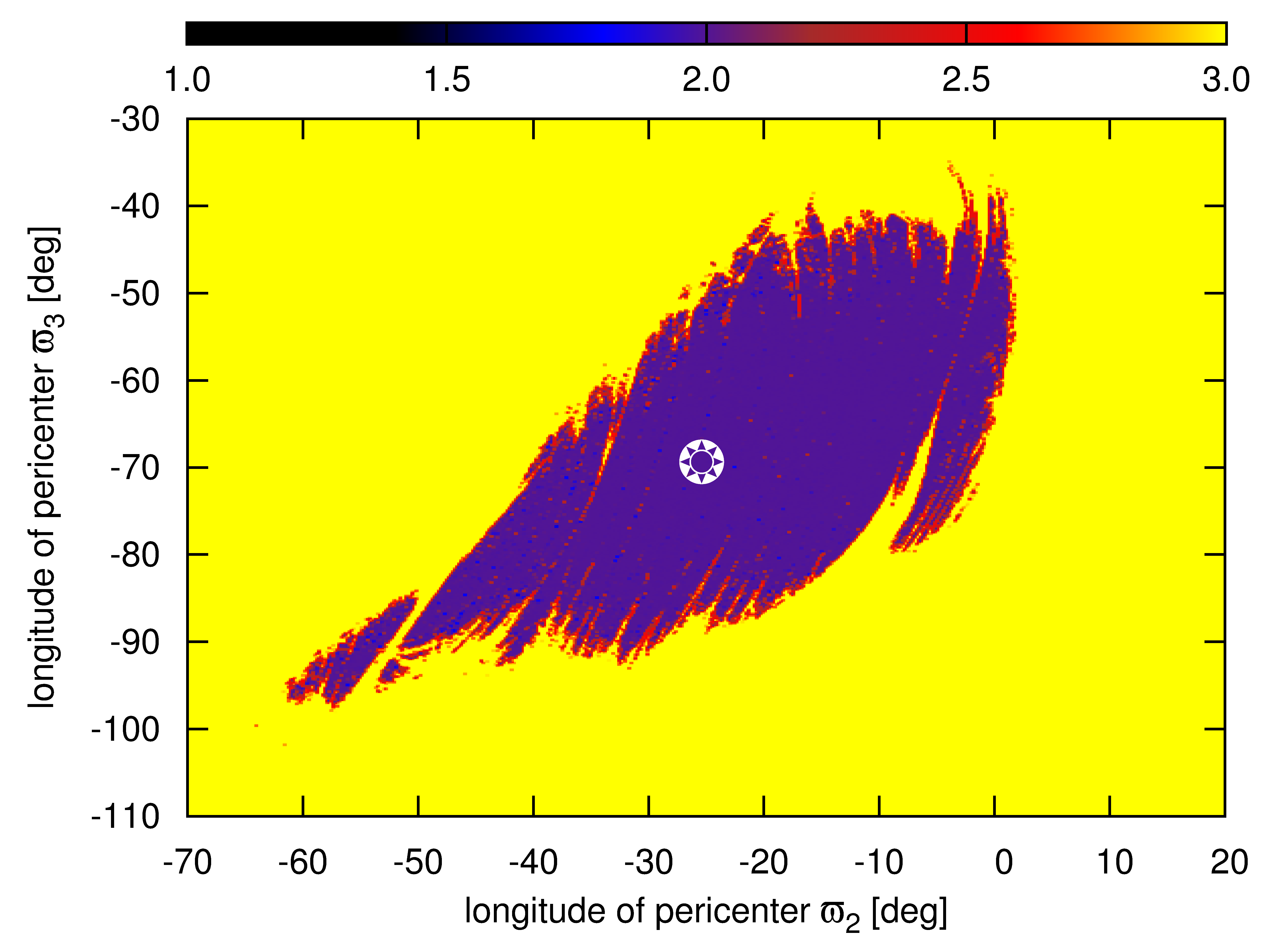
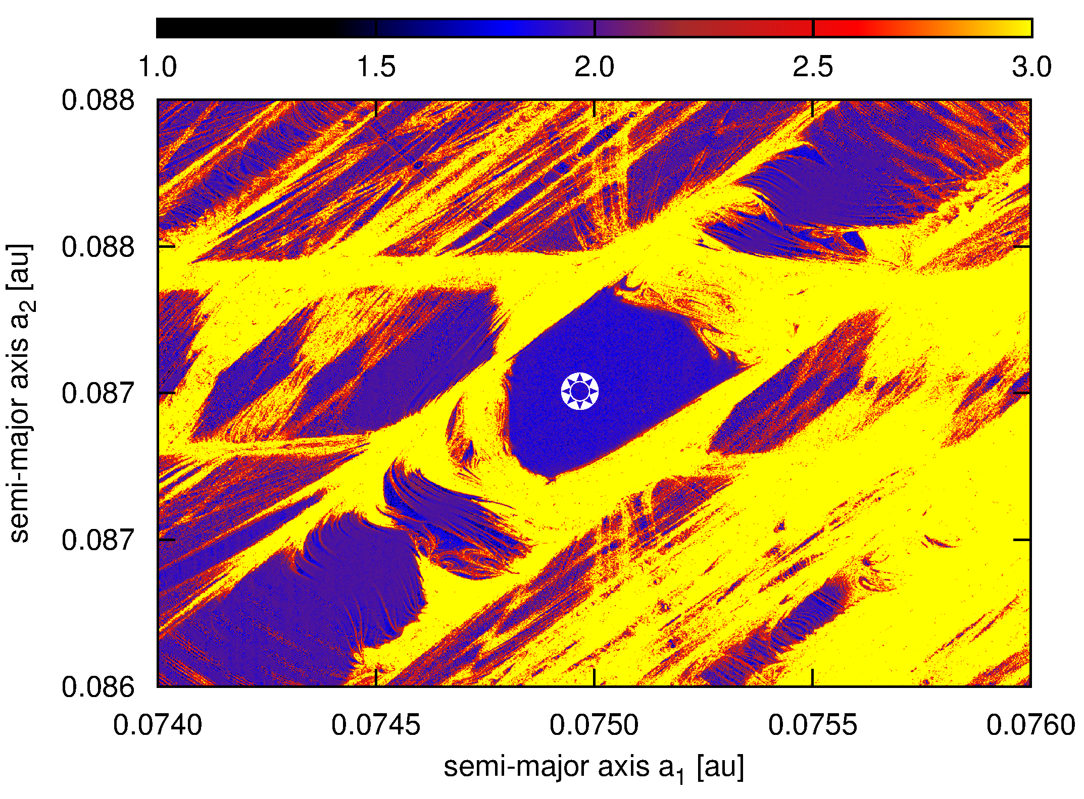
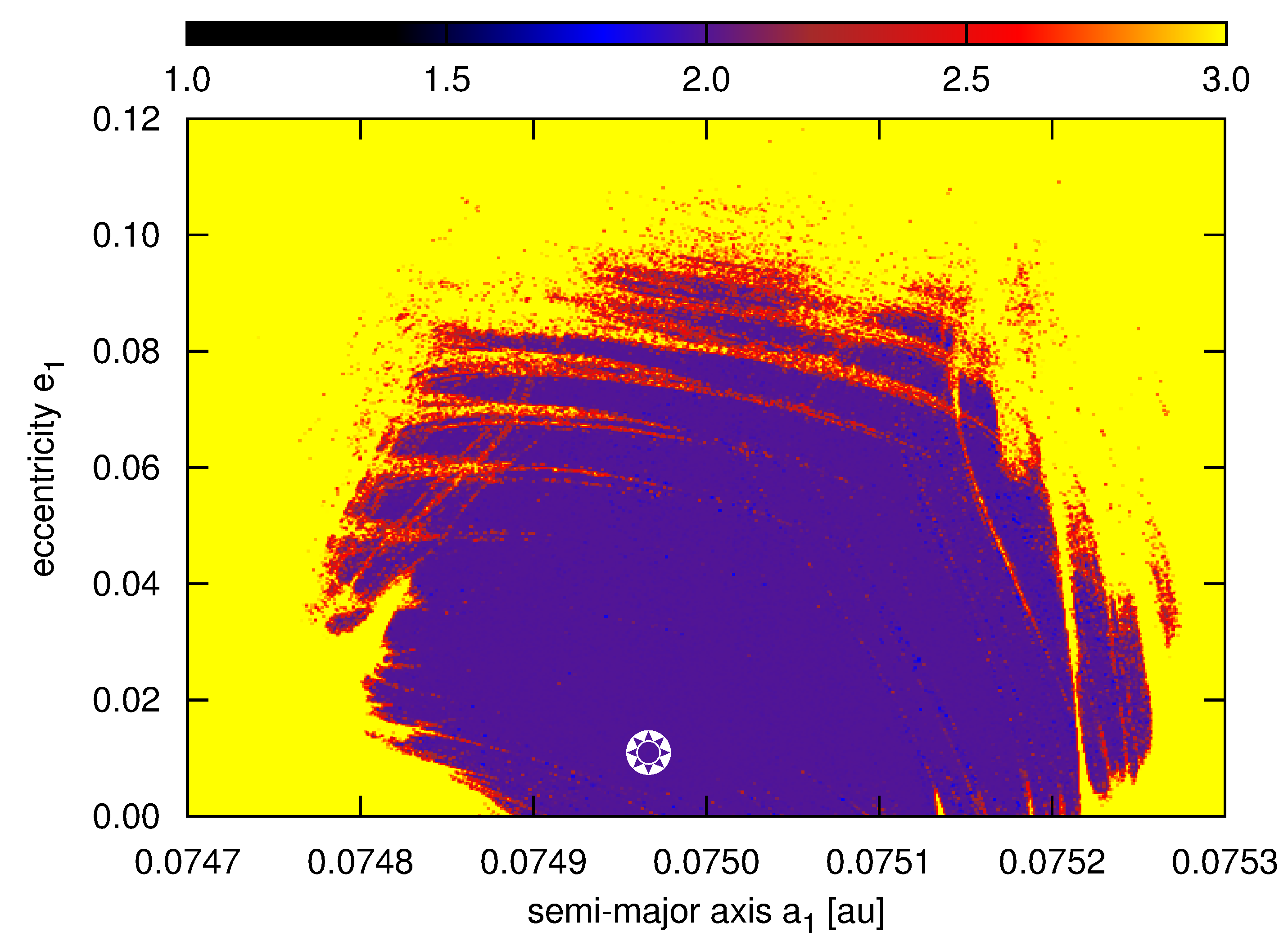
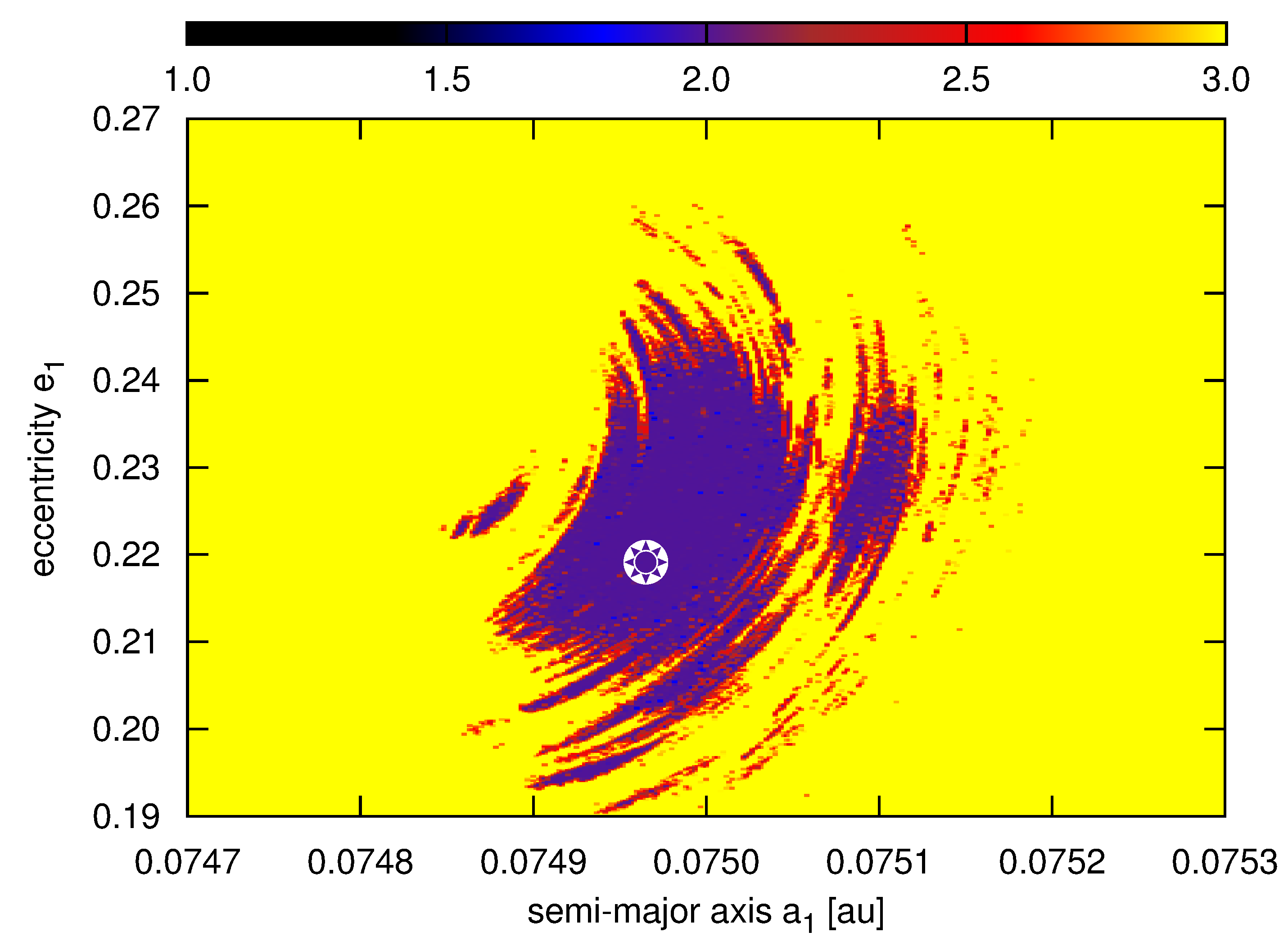
Figure 4: Dynamical maps for the best-fitting three-body MMRs models in Tab. 1. The MEGNO $\langle Y\rangle\sim 2$ indicates a regular (long-term stable) solution marked with black/dark blue colour, $\langle Y\rangle$ much larger than $2$, up to $\gtrsim 5$ indicates a chaotic solution (yellow). The integration time of each initial condition is 32,000 yr ($\sim 10^{6}\times P_{{\mbox{\scriptsize 3}}}$) besides the bottom-left panel where the integration time is 80 yr. The asterisk symbol means the position of the nominal model. The top-row: dynamical maps for Fit I in Tab. 1. Subsequent maps are for the $(a_{{\mbox{\scriptsize 1}}},a_{{\mbox{\scriptsize 2}}})$–, $(a_{{\mbox{\scriptsize 1}}},e_{{\mbox{\scriptsize 1}}})$– and $(\varpi_{2},\varpi_{3}$)–planes. The bottom-row: $(a_{{\mbox{\scriptsize 1}}},a_{{\mbox{\scriptsize 2}}})$–map for Fit I with reduced integration time, $(a_{{\mbox{\scriptsize 1}}},e_{{\mbox{\scriptsize 1}}})$–plane for Fit II, and $(a_{{\mbox{\scriptsize 1}}},e_{{\mbox{\scriptsize 1}}})$–map for the true Laplace resonance in moderate–eccentricity region. See the text for details.

6 Acknowledgements

We thank the anonymous reviewer for comments that improved this paper. This work has been supported by Polish National Science Centre MAESTRO grant DEC-2012/06/A/ST9/00276. K.G. thanks the Poznań Supercomputer and Network Centre (PCSS, Poland) for computing resources (grant No. 195) and a generous support.

Supplementary online material

Figure 5: One– and two–dimensional projections of the posterior probability distribution for all free parameters of the TTV model. The MCMC chain length is 1,024,000 iterations in each of 512 different instances selected in a small ball around a solution found with the genetic algorithms. First transit epochs $T_{b,c,d}$ and orbital periods $P_{b,c,d}$ are expressed in days, planetary masses $m_{b,c,d}$ are expressed in Earth masses, and the uncertainty correction term $\sigma_{f}$ is given in minutes ($b\equiv 1,c\equiv 2,d\equiv 3$ are indices of subsequent planets).

References

- Agol et al. (2005) Agol E., Steffen J., Sari R., Clarkson W., 2005, MNRAS, 359, 567
- Baluev (2009) Baluev R. V., 2009, MNRAS, 393, 969
- Batygin et al. (2015) Batygin K., Deck K. M., Holman M. J., 2015, AJ, 149, 167
- Carter et al. (2011) Carter J. A., Fabrycky D. C., Ragozzine D., Holman M. J., Quinn S. N., et al. 2011, Science, 331, 562
- Charbonneau (1995) Charbonneau P., 1995, ApJS, 101, 309
- Cincotta et al. (2003) Cincotta P. M., Giordano C. M., Simó C., 2003, Physica D Nonlinear Phenomena, 182, 151
- Deck et al. (2014) Deck K. M., Agol E., Holman M. J., Nesvorný D., 2014, ApJ, 787, 132
- Fabrycky et al. (2014) Fabrycky D. C., Lissauer J. J., Ragozzine D., Rowe J. F., Steffen J. H., Agol E., Barclay T., et al. 2014, ApJ, 790, 146
- Foreman-Mackey et al. (2013) Foreman-Mackey D., Hogg D. W., Lang D., Goodman J., 2013, PASP, 125, 306
- Froeschlé et al. (2000) Froeschlé C., Guzzo M., Lega E., 2000, Science, 289, 2108
- Goodman & Weare (2010) Goodman J., Weare J., 2010, Comm. Apl. Math and Comp. Sci., 1, 65
- Goździewski & Migaszewski (2014) Goździewski K., Migaszewski C., 2014, MNRAS, 440, 3140
- Guzzo (2006) Guzzo M., 2006, Icarus, 181, 475
- Lee et al. (2013) Lee M. H., Fabrycky D., Lin D. N. C., 2013, ApJ, 774, 52
- Libert & Tsiganis (2011) Libert A.-S., Tsiganis K., 2011, Celestial Mechanics and Dynamical Astronomy, 111, 201
- Marcy et al. (2001) Marcy G. W., Butler R. P., Fischer D., Vogt S. S., Lissauer J. J., Rivera E. J., 2001, ApJ, 556, 296
- Marois et al. (2010) Marois C., Zuckerman B., Konopacky Q. M., Macintosh B., Barman T., 2010, Nature, 468, 1080
- Martí et al. (2013) Martí J. G., Giuppone C. A., Beaugé C., 2013, MNRAS, 433, 928
- Moore et al. (2013) Moore A., Hasan I., Quillen A. C., 2013, MNRAS, 432, 1196
- Mullally et al. (2015) Mullally et al. 2015, ApJS, 217, 31
- Murray & Holman (1999) Murray N., Holman M., 1999, Science, 283, 1877
- Papaloizou (2015) Papaloizou J. C. B., 2015, International Journal of Astrobiology, 14, 291
- Papaloizou & Terquem (2010) Papaloizou J. C. B., Terquem C., 2010, MNRAS, 405, 573
- Quillen (2011) Quillen A. C., 2011, MNRAS, 418, 1043
- Quillen & French (2014) Quillen A. C., French R. S., 2014, MNRAS, 445, 3959
- Rivera et al. (2010) Rivera E. J., Laughlin G., Butler R. P., Vogt S. S., Haghighipour N., Meschiari S., 2010, ApJ, 719, 890
- Rowe et al. (2015) Rowe J. F., Coughlin J. L., Antoci V., Barclay T., Batalha N. M., Borucki W. J., Burke C. J., et al. 2015, ApJS, 217, 16
- Ruciński et al. (2010) Ruciński M., Izzo D., Biscani F., 2010, Parallel Computing, 10, 555
- Showalter & Hamilton (2015) Showalter M. R., Hamilton D. P., 2015, Nature, 522, 45
- Sinclair (1975) Sinclair A. T., 1975, MNRAS, 171, 59
- Smirnov & Shevchenko (2013) Smirnov E. A., Shevchenko I. I., 2013, Icarus, 222, 220
- Steffen et al. (2012) Steffen J. H., Fabrycky D. C., Ford E. B., Carter J. A., Désert J.-M., et al. 2012, MNRAS, 421, 2342
- Terquem & Papaloizou (2007) Terquem C., Papaloizou J. C. B., 2007, ApJ, 654, 1110
- Wang et al. (2012) Wang S., Ji J., Zhou J.-L., 2012, ApJ, 753, 170