ExoData: A Python package to handle large exoplanet catalogue data

Abstract

Exoplanet science often involves using the system parameters of real exoplanets for tasks such as simulations, fitting routines, and target selection for proposals. Several exoplanet catalogues are already well established but often lack a version history and code friendly interfaces. Software that bridges the barrier between the catalogues and code enables users to improve the specific repeatability of results by facilitating the retrieval of exact system parameters used in an articles results along with unifying the equations and software used. As exoplanet science moves towards large data, gone are the days where researchers can recall the current population from memory. An interface able to query the population now becomes invaluable for target selection and population analysis.

ExoData is a Python interface and exploratory analysis tool for the Open Exoplanet Catalogue. It allows the loading of exoplanet systems into Python as objects (Planet, Star, Binary etc) from which common orbital and system equations can be calculated and measured parameters retrieved. This allows researchers to use tested code of the common equations they require (with units) and provides a large science input catalogue of planets for easy plotting and use in research. Advanced querying of targets are possible using the database and Python programming language. ExoData is also able to parse spectral types and fill in missing parameters according to programmable specifications and equations. Examples of use cases are integration of equations into data reduction pipelines, selecting planets for observing proposals and as an input catalogue to large scale simulation and analysis of planets.

ExoData is a Python package available freely on GitHub. It is open source and community contributions are encouraged. The package can be easily installed using pip install exodata, detailed setup information is provided within.

PROGRAM SUMMARY

Manuscript Title: ExoData: A Python package to handle large exoplanet catalogue data
Authors: Ryan Varley
Program Title: ExoData
Journal Reference:
Catalogue identifier:
Licensing provisions: GPL 3.0
Programming language: Python 2.7, 3.4, 3.5
Computer: Any
Operating system: Any
RAM: less than 200MB
Keywords: Exoplanets , Catalogues , Interface
Classification: 1.7 Stars and Stellar Systems
External routines/libraries: numpy, quantities, matplotlib, requests, astropy, seaborn
Nature of problem:
Being able to use exoplanet catalogue values in code including where there may be incomplete and incorrectly formatted values. Also being able to use the whole catalogue data at once, both for user querying, visualisation and in large simulation programs.
Solution method:
An interface to access the catalogue including filling in missing values and parsing of the catalogue data. Creating an API usable by both humans and other code, implementation of commonly used exoplanet equations, a plotting library.
Running time:
A few seconds depending on the task.

1 Introduction

The field of exoplanets is rapidly expanding with current population now in the thousands and new measurements published increasingly frequently. A catalogue of Exoplanets is necessary to keep track of these systems and their parameters, ideally being open and editable by all with a version history to enable researchers to reproduce results using the exact same values. This is especially important in large scale simulations and other work on multiple targets where a catalogue version may be more easily given over individual values and sources.

A second obstacle lies in the interface between the catalogue and the code. Such an interface can add value in its ability to calculate values using published equations, easily generate plots, estimate parameters, while keeping the catalogue up to date. It can also take into account all the fringe cases which can trip up a standard loading code (such as certain missing values and planets without a host star). The ability to replicate the catalogue is further enhanced through quoting both a catalogue and interface version. The exact parameters used for every target in the catalogue can then be easily obtained including any calculated parameters and estimations by ExoData. This tool then allows instant access to the exact parameters used in a paper.

1.1 Open Exoplanet Catalogue

The Open Exoplanet Catalogue (OEC, Rein, 2012) is an open-source, version controlled catalogue of exoplanets and their system parameters. It is hierarchical, preserving the format of the system (including binary star layouts). OEC uses git for version control and the catalogue exists as a series of XML files (one per system). This format makes OEC much more diverse than most other exoplanet catalogues by letting users create their own ‘forks’ of the catalogue where they can make their own changes and adaptations whilst still able to receive updates from the original. The advantages of version control include being able to see the exact changes made to each version, easily roll back the catalogue to any previous state and report the exact version of the catalogue your using to other researchers (using the commit SHA-1).

The open nature of the catalogue means that anyone can download the full database and history of the catalogue, contribute their own changes and set up their own branched versions.

2 Exoplanet Background Theory

An exoplanet is a planet that orbits a star other than the Sun. We can describe a simple exoplanet system with a planet orbiting a star with a stellar radius of $R_{\star}$ stellar mass of $M_{\star}$ planetary radius $R_{p}$, planetary mass $M_{p}$ and semi-major axis of the orbit $a$.

2.1 Describing the star

The stellar luminosity $L_{\star}$ is given by the Stefan-Boltzmann equation applied to the surface area of a sphere,

$$L_{\star}=4\pi R^{2}_{\star}\sigma T^{4}_{\star}$$ (1)

where $\sigma$ is the Stefan-Boltzmann constant. Stellar temperature can be estimated using the stellar mass-radius relation described in Cox (2000):

$$R_{\star}=kM^{x}_{\star}$$ (2)

where k and x are constants for each stellar sequence. We can also describe stellar temperature using the main sequence relationship

$$T_{\star}=5800\times M_{\star}^{0.65}.$$ (3)

The stars luminosity distance $d$ (with negligible extinction) is given by rearranging the absolute magnitude relation

$$m-M=5\log_{10}{d}-5$$ (4)

where $m$ is the apparent magnitude and $M$ is the absolute magnitude. Whilst $m$ is easily measured and commonly known $M$ is often undefined. We can estimate $M$ for a star using an absolute magnitude lookup table based on spectral type.

In cases where we do not have a measured stellar magnitude in the band required but do have a measured value for another band we can use the conversion factors given in table A5 of Kenyon and Hartmann (1995) to convert between magnitudes based on the stellar spectral type.

2.2 Describing the planet

We can infer the period of the orbit $P$ using Kepler’s third law

$$P=\sqrt{\frac{4\pi^{2}a^{3}}{G\left(M_{\star}+M_{p}\right)}}$$ (5)

where $G$ is the gravitational constant. We can rewrite this in terms of the semi-major axis given the stellar mass and period. Note that the $M_{p}$ term is often excluded as $M_{\star}\gg M_{p}$.

$$a=\left(\frac{P^{2}GM_{*}}{4*\pi^{2}}\right)^{1/3}$$ (6)

The semi-major axis can additionally be inferred from the temperature of the planet $T_{p}$ and host star $T_{\star}$ given an albedo for the planet $A_{p}$ and a greenhouse constant $\epsilon$ (Tessenyi et al., 2012):

$$a=\sqrt{\frac{1-A_{p}}{\epsilon}}\frac{R_{\star}}{2}\left(\frac{T_{\star}}{T_{p}}\right)^{2}.$$ (7)

The mean planetary effective temperature can be expressed by evaluating the radiation in and out of the planet with a greenhouse effect contribution $\epsilon$ using a rearranged version of Eqn. 7

$$T_{pl}=T_{\star}\left(\sqrt{\frac{(1-A)}{\epsilon}\frac{R_{\star}}{2a}}\right)^{1/2}.$$ (8)

From Newton’s law of Gravitation we can calculate the surface gravity of the planet

$$g=\frac{GM}{R_{p}^{2}}.$$ (9)

This can be expressed as $\log{g}$, the base 10 $\log$ of $g$ in CGS units.

If the mass of a planet is unknown, according to mass-radius relationships of known exoplanets (e.g. Grasset et al. (2009)) the mass can be crudely estimated for a given planetary radius by assuming the density of the planetary class it is likely to be in. For this purpose we infer super-Earths as Earth density, and Jupiter and Neptune like planets with their respective densities. Assumed values are described later in Table 2 but are easily programmable (see assumptions module section 4.4).

The scale height $H$ is the increase in altitude for which the atmospheric pressure decreases by a factor of e.

$$H=\frac{kT_{p}}{\mu g}$$ (10)

where $\mu$ is the mean molecular weight of the planetary atmosphere and $g$ is the planetary surface gravity.

2.3 Transiting Exoplanets

An exoplanet transits if it can be observed passing in front of its host star. During a transit the planet occults light from the star with the change in flux at mid transit known as the transit depth. The transit depth can be estimated as the square of the ratio of the planetary radius to the stellar radius (however, it is possible for a planet to graze the limb creating a partial transit).

The impact factor $b$ is the projected distance between the planet and star centres during mid transit and it is described as (Seager and Mallen-Ornelas, 2003):

$$b\equiv\frac{a}{R_{*}}\cos{i}.$$ (11)

If the orbit is circular, we can calculate the duration of the transit $T_{\text{14}}$ from first to last contact using Eqn. 3 from (Seager and Mallen-Ornelas, 2003):

$$T_{\text{14}}=\frac{P}{\pi}\arcsin\left(\frac{R_{\star}}{a}\frac{\sqrt{(1+k)^{2}+b^{2}}}{\sin{a}}\right)$$ (12)

where k is $\frac{R_{p}}{R_{s}}$. If the planet has an eccentric orbit where the exact solution is more complex we adopt the approximation described by Kipping (2011):

$$T_{14}=\frac{P}{\pi}\frac{\varrho^{2}_{c}}{\sqrt{1-e^{2}}}\arcsin{\left(\frac{\sqrt{1-a_{R}^{2}\varrho_{c}^{2}\cos^{2}{i}}}{a_{R}\varrho_{c}\sin{i}}\right)}$$ (13)

where $a_{R}=(a/R_{\star})$ and $\varrho_{c}$ is the planet-star separation at the moment of mid-transit in units of stellar radii

$$\varrho_{P,T}(f_{p})=\frac{1-e^{2}_{P}}{1+e_{P}\sin(\omega)}$$ (14)

where $\omega$ is the argument of pericentre and $b_{P,T}$ is the adjusted impact parameter described by

$$b_{P,T}=(a_{P}/R_{\star})\varrho_{P,T}\cos{i}.$$ (15)

3 Installation

ExoData is a Python package tested on Python versions 2.7, 3.4 and 3.5. The easiest way to get the package is through the Python packaging tool pip,

pip install exodata

Alternatively the source code can be downloaded from https://github.com/ryanvarley/exodata. The package can then be installed by the following from the command line in the package directory.

python setup.py install

The package has a test suite which can be used to verify the package is working as expected. To run the tests use

python setup.py test

You can choose to use the package without downloading your own copy of the catalogue, instead choosing to automatically fetch the latest version each time. If you want to use your own version you will need to download a version of the Open Exoplanet Catalogue (OEC) to your machine. The easiest way to do this and keep the catalogue up to date is through git. Move to the folder you want to store the catalogue in and then

git clone https://github.com/OpenExoplanetCatalogue/open_exoplanet_catalogue.git

You can then ‘import exodata’ in Python and setup the catalogue.

import exodata
databaseLocation = "/open-exoplanet-catalogue/systems/"
exocat = exodata.OECDatabase(databaseLocation)

where databaseLocation should be the full path to the systems folder in the OEC directory or any other folder that contains OEC style XML files you want to use.

To update the catalogue move to the folder where you downloaded the catalogue and type

git pull origin master

When using ExoData in publications you should give the commit SHA-1 of the OEC version used and the ExoData version number. This document was created with the Open Exoplanet Catalogue (dc8c08a4ba0c64dd039e96c801d12f17c82a7ff3, 1st May 2016) using ExoData Version 2.1.5.

3.1 Dependencies

The following dependencies are required to run ExoData. They are installed automatically by setuptools if required when following the above installation procedure.

• numpy

• matplotlib

• quantities (Product Quantities)

• requests

• seaborn

4 Usage

ExoData is split into a series of modules dealing with the exoplanet database, equations, plots and units (see Table 1 for a list with descriptions).

Module	Descrption
Assumptions	Holds classification assumptions such as at what mass or radius a planet is defined as a super-Earth.
Astroclasses	Classes for the System, Binary, Star and Planet object types.
Astroquantities	Expands the Product Quantities Python package with astronomical units like Solar Radius and compound units such as $g/cm^{3}$.
Database	Holds the database class and the various search methods.
Equations	Implementation of exoplanet related equations including orbital equations, planet and star characterisations and estimations.
Example	Generate example systems for testing code.
Flags	Each object has a flag object attached which lets you know which assumptions have been made such as ‘calculated temperature’.
Plots	Plot functions for common plot types that can be used to to easily display data from the catalogue.

Table 1: Table showing the modules available in ExoData and what they are used for.

The code contains 5 main objects types, the database which holds all objects and provides functionality (such as searching) and the astronomical objects (Systems, Binaries, Stars and Planets). Moons and other types can be easily added when needed.

Like the Open Exoplanet Catalogue (OEC), the full structure of a system is preserved. Planets are children of the star (or binary) they orbit, stars are grouped in binaries where present and binaries can exist within a binary. This offers a significant structural advantage over most linear formats.

Note that the examples that follow in this paper display the raw output from the console which means most numbers are displayed showing 11 decimal places which include any floating point errors and so should not be taken as the true uncertainty in the measurement.

4.1 As a catalogue interface

The database is initialised by providing the OECDatabase object with the catalogue location on your machine.

import exodata

# Either using your own catalogue version
databaseLocation = "/open_exoplanet_catalogue/systems/"
exocat = exodata.OECDatabase(databaseLocation)

# OR downloading the latest version each time
exocat = exodata.load_db_from_url()

The exocat variable now contains the initialised database which can be accessed in several ways. There are lists for each type of object (i.e. exocat.planets, exocat.stars etc), a dictionary for each object (i.e. exocat.planetDict) and a list of transiting planets (exocat.transitingPlanets).

You can retrieve a particular planet either by searching or giving the exact name.

>>> exocat.planetDict["Gliese 1214 b"]
Planet("Gliese 1214 b")

>>> exocat.searchPlanet("gj1214b")
Planet("Gliese 1214 b")

We can then traverse the hierarchy for the planet.

>>> kepler10b = exocat.planetDict["Kepler-10 b"]
>>> kepler10b.parent
Star("Kepler-10")

>>> kepler10 = kepler10b.star
>>> kepler10.planets
Planet("Kepler-10 b"), Planet("Kepler-10 c")]

>>> kepler10b.system
System("Kepler-10")

4.1.1 Retrieving Values

With an object selected we can query information from the database.

>>> gj1214b = exocat.planetDict["Gliese 1214 b"]
>>> print gj1214b.R  # planetary radius
array(0.2525) * R_j

>>> print gj1214b.a  # orbit semi-major axis
array(0.01488) * au

>>> print gj1214b.star.M  # stellar mass of host star
array(0.176) * M_s

The returned values are Product Quantities objects that act like floats or more precisely a single value numpy array but with a few extra features such as unit rescaling and dimensionality checking (see section 4.2).

>>> import exodata.astroquantities as aq
>>> print gj1214b.R.rescale(aq.R_e)  # rescale to earth radii
array(2.770762439177523) * R_e

>>> print gj1214b.M / gj1214b.R  # mass / radius ratio
array(0.07722772277227723) * M_j/R_j

In addition to retrieving values straight from the database we can also directly call some equations from the exodata.equations module with the variables pre-filled (see B for a full list).

>>> print gj1214b.calcDensity()
array(1.6067887724162309) * g/cm**3

>>> print gj1214b.calcTemperature()
array(606.022512904359) * K

4.1.2 Querying the Database

Querying can be performed on object list in the form of Python for loops or list comprehensions. ExoData will return numpy.nan if a value is absent to avoid breaking loops and comparisons with exodata.MissingValue exceptions. MissingValue Exceptions will still be recorded in the logfile and so can be examined if needed. An example of such a query is returning the planets discovered using the radial velocity method.

>>> detected_by_rv = [planet for planet in exocat.planets
                  if planet.discoveryMethod =="RV"]
>>> print len(detected_by_rv) # number of planets detected by RV
658

>>> print detected_by_rv[:2]  # first 2 planets detected by RV (alphabetical)
[Planet("11 Com b"), Planet("11 UMi b")]

You can use this same method to get a list of every planets radius. Note that some values will return as numpy.nan, we can filter these in the initial query so a normal numpy.mean will work.

>>> import numpy as np
>>> radius_list = [planet.R for planet in exocat.planets
               if planet.R is not np.nan]
>>> print np.mean(radius_list)
0.454992066547

More advanced queries with additional if clauses can be used to filter the results further. For example, to display all planets with a planetary radius between 1.83 and 1.9 Jupiter radii.

>>> print [planet for planet in exocat.planets
        if planet.R is not np.nan
        and 1.83*aq.R_j < planet.R < 1.9*aq.R_j]
[Planet("KELT-8 b"), Planet("TrES-4 A b")]

For complicated queries a Python for loop may be clearer. Here we show all planets with a radius between 1.5 and 1.7 Jupiter radii that were discovered by the transit method and have an orbital eccentricity greater than 0.1.

>>> planet_list = []
>>> for planet in exocat.planets:
        if 1.5*aq.R_j < planet.R < 1.7*aq.R_j:
            if planet.discoveryMethod == "transit":
                if planet.e > 0.1: # eccentric
                    planet_list.append(planet)
>>> print planet_list
[Planet("HATS-3 b"), Planet("Kepler-447 b"), Planet("WASP-90 b")]

4.2 Units

In exodata, all equations use and require units. This means values can easily be rescaled and all equations are dimensionally checked. Units are provided through the product quantities package which provides all the standard units and constants provided by the National Institute of Standards and Technology (NIST). Some astronomical units (see table 9 for the list of values and sources) are added through the internal exodata.astroquantities module which imports all Product Quantities units for ease of use. We can then import the units from both modules using:

>>> import exodata.astroquantites as aq

Product Quantities adds units to numbers as a special numpy array type. A unit is added to a value by multiplying the values by the unit i.e.

>>> planetRadius = 10 * aq.R_j

Product Quantities provides several methods for dealing with values with a unit. Rescaling can be done using the .rescale method e.g. to rescale solar mass to units of Earth’s mass.

>>> print (1.99e+30 * aq.kg).rescale(aq.M_e)
array(333211.10011570295) * M_e

Units can be converted to their unit-less counterparts (i.e for passing to code without unit support) by wrapping them in a float() or np.array() argument. You should always remove units with a rescale to ensure the value is in the unit you expect.

>>> value = 100 * pq.cm
>>> print float(x.rescale(pq.m))
1.0

4.3 Equations

The equations module implements the equations described in section 2 as Python classes. The classes take input of every variable bar one and will output the variable left out. They therefore implement all permutations of the equation with respect to the variables.

As an example we choose the equation Kepler’s Third Law (Eqn. 5), a full list of implemented equation classes and the equation they draw from are given in A. The function is called KeplersThirdLaw and taking the values for GJ 1214 b we can calculate the period.

>>> from exodata.equations import KeplersThirdLaw
>>> KeplersThirdLaw(a=0.01488*aq.au, M_s=0.176*aq.M_s).P
array(1.579696141940911) * d

Similarly, given the other two values we can calculate the missing one.

>>> KeplersThirdLaw(a=0.015*aq.au, P=1.58*aq.d).M_s
array(0.18022315673929146) * M_s

>>> KeplersThirdLaw(M_s=0.176*aq.M_s, P=1.58*aq.d).a
array(0.01488190807285067) * au

4.4 Assumptions

The assumptions module handles how non universally defined parameters are set along with how some missing values may be filled. This include how planets are categorised (i.e. super-Earth) and allows researchers to use their own definitions for these planet classes along with adding new classes.

By default ExoData sets these to commonly assumed values. Table 2 shows how a planet is classified as being a Jupiter, Neptune or super-Earth along with the assumptions of mean molecular weight and density where required. For the mass limits we use the classification boundaries adopted by (Tinetti et al., 2013).

	Jupiter	Neptune	Super-Earth
Mass ($M_{\oplus}$)	$>$ 20	$>$ 10	$<$ 10
Radius ($R_{\oplus}$)	$>$ 6	$>$ 4	$<$ 1.8
Density (g/$cm^{3}$)	1.3	1.6	4
Mean Molecular Weight (a.m.u)	2.0	2.3	18

Table 2: Default assumptions of planet values per classification. We use the mass to classify a planet first, if the mass is missing we then use the radius. Densities are Jupiter, Neptune and Earth densities. All these values can be changed in the program (see text).

Assumptions are implemented to make it easy to change these limits and also add more by editing the assumptions dictionary located at exodata.assumptions.planetAssumptions.

This dictionary has the keys ‘masstype’, ‘radiusType’ and ‘tempType’ which define how a planet is classified. Each key is a list of rules defining a separate type of planet in the format (upperlimit, name). For example we have defined the following for ‘massType’

[(10 * aq.M_e, "Super-Earth"),
 (20 * aq.M_e, "Neptune"),
 (float("inf"), "Jupiter")]

Setting the last rule to infinity defines the last rule having no upper limit. The first rule is assumed to have no lower limit. The rules should be listed in descending order of magnitude and can be added to, modified or removed as necessary.

The dictionary also has keys defining certain value assumptions based upon the classifications set previously. These are ‘mu’, ‘albedo’ and ‘density’. These are fed into the planet classes and can be used in calculations if needed. Instead of containing a list they contain a dictionary which takes a classification ‘name’ defined previously and provides a value for that class. Both the ‘mu’ and ‘density’ keys are defined by mass and radius types, for example:

{"Super-Earth": 18 * aq.atomic_mass_unit,
 "Neptune"    : 2.3 * aq.atomic_mass_unit,
 "Jupiter"    : 2 * aq.atomic_mass_unit}

Again these values can be changed and modified as needed and new rules added for any new classes added to the previous set of rules.

4.5 Flags

When a catalogue value is missing it is calculated or estimated using an appropriate equation in exodata.equations if possible. While this is in many cases desirable some assumptions are more accurate than others and it is useful to know when a parameter has been filled. To this end we raise a flag in an object if a certain actions have occurred. The list of flags and the functions that raise them is shown in Table 3.

Table 3: List of flags and the functions that raise them when a parameter is missing and is calculated or estimated instead.

Flag	Calculated using
Estimated Mass	estimateDistance()
Calculated SMA	calcSMA()
Fake	Any planet that is in the ‘Fake Planets’ list in the xml files
Estimated Distance	estimateDistance()
Estimated magV	magV (V magnitude)
Calculated Period	calcPeriod()
Calculated Temperature	calcTemperature()

For example when we ask for the semi-major axis of a planet (planet.a) and a value is not recorded in the catalogue the interface will attempt to calculate it using Kepler’s Third Law. If it is successful the value will be returned and the flag ‘Calculated SMA’ will be raised. A list of flags that have been raised in an object can be seen by looking at the flags object of planet or star class (i.e planet.flags).

If instead you want only raw catalogue values with no attempt at filling in missing values you can turn off this behaviour using by setting params.estimateMissingValues=False.

4.6 Plotting with ExoData

ExoData includes some graphing functions for easily displaying catalogue data. The main types of plots available are parameter against parameter and the number of planets per parameter bin. The general format is setting up the plot class with a list of objects to plot and then calling a plot function of the type you want with any other visual arguments. The plot style can be changed using standard matplotlib styles. In our examples we used the ‘whitegrid’ style by the Seaborn module. In order for plots to be visible in the command line you may need to import matplotlib and use the plt.show() after calling a plot function.

4.6.1 Number of planets by discovery method

This plots the number of planets discovered by each type of discovery method per year as a stacked bar chart. The format is

exodata.plots.DiscoveryMethodByYear(planet_list, methods_to_plot
  ).plot(method_labels)

where planet_list is a list of planet objects to plot, methods_to_plot is the discovery methods to include (in OEC syntax) and method_labels are the labels to use in the legend for each discovery method. We can create a plot of the radial velocity and transit discovery methods with the following (shown in Fig. 1).

exodata.plots.DiscoveryMethodByYear(
    exocat.planets,
    methods_to_plot=("RV", "transit", "Other")
).plot(
    method_labels=("Radial Velocity", "Transit Method", "Other"))

By specifying ‘Other’ as a discovery method ExoData will group all methods not specified into this category on the plot.

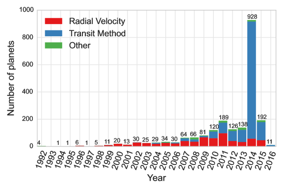
Figure 1: Example plot that can be generated with DiscoveryMethodByYear in the ExoData plotting module. See text for description.

4.6.2 Plotting a parameter against another

This type of plot takes a measured or calculated parameter of the planet, star, binary or system and displays it against another. The format is

exodata.plots.GeneralPlotter(list_of_objects,
  x_param, y_param).plot(*plot_arguments)

where list_of_objects is a list of planets, stars or binaries you want to be plotted and the x and y parameters refer to the string of the parameter you want. For example, to plot planet mass against radius (Fig. 2a)

exodata.plots.GeneralPlotter(
    exocat.planets, "R", "M", yaxislog=True).plot()
plt.xlim(-0.1, 2.1)

where R would retrieve the planetary radius (planet.R) and M the planetary mass. Extra options are available to change the plot including log scale, changing the unit used (conversion is performed on the fly), marker colour and size and using parameters from a related object such as the parent star. Some more examples are shown in Fig. 2.

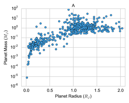
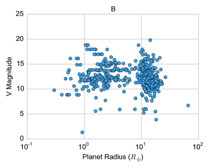
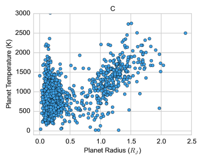
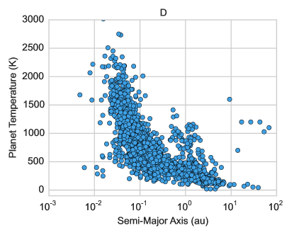
Figure 2: Example plots that can be generated with GeneralPlotter in the ExoData plotting module. See text for descriptions.

4.6.3 Number of planets per parameter bin

These plots take input of the object list, the parameter to plot and the bin limits to produce a histogram-like plot or pie chart. The format is

exodata.plots.DataPerParameterBin(
    list_of_objects, parameter, bin_limit
    ).plotBarChart(*plot_arguments)

Less than / greater than limits can be made by setting the first or last limit to float(‘-inf’) or float(‘inf’) i.e. the following generates Fig. 3A.

exodata.plots.DataPerParameterBin(
    exocat.planets, "e",
    (0, 0, 0.05, 0.1, 0.2, 0.4, float("inf"))
    ).plotBarChart(label_rotation=45)

You can alternatively plot bar charts by typing .plotPieChart() instead of .plotBarChart() (see Fig. 3B).

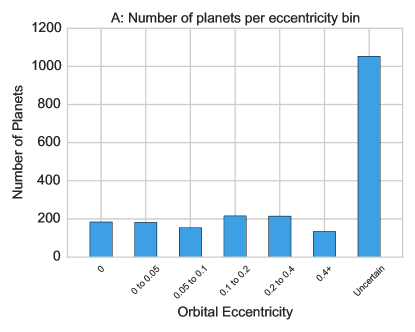
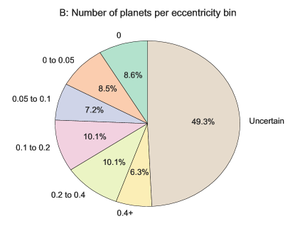
Figure 3: Example plots that can be generated with DataPerParameterBin in the ExoData plotting module. See text for description.

5 Conclusion

ExoData provides a rounded tool for researchers wishing to use parameters of an exoplanet or exoplanetary system in code. Uses of the module include querying the exoplanet database for targets for observing proposals, running planets through a simulator and easy access to the catalogue for population statistics.

By using a version controlled catalogue like the Open Exoplanet Catalogue and the ExoData interface researchers can more easily verify published results by easily obtaining the exact same planet and system parameters used by quoting both the catalogue and interface version. This is different from most catalogues which only show the latest version of which many unknown values may have changed. The interface builds upon the catalogue by making it easier to access parameters, calculate values and query the database.

6 Acknowledgements

This work is supported by a UCL IMPACT studentship and STFC grant code ST/P000282/1.

Appendix A List of equations

Table 4: List of equations in the equations module

Function name	Function Arguments	Description
ScaleHeight	T_eff, mu, g, H	Eqn. 10
MeanPlanetTemp	A, T_s, R_s, a, epsilon, T_p	Eqn. 7
StellarLuminosity	R, T, L	Eqn. 1
KeplersThirdLaw	a, M_s, P, M_p	Eqn. 5
SurfaceGravity	M, R, g	Eqn. 9
Logg	M, R, logg	base 10 log of SurfaceGravity
TransitDepth	R_s, R_p, depth	square of the ratio of the planetary radius to the stellar radius
Density	M, R, Density	Density = Mass/Volume
TransitDuration	P, a, Rp, Rs, i, e, w	Eqn. 13
ImpactParameter	a, R_s, i, b	Eqn. 11
transitDurationCircular	P, R_s, R_p, a, i	Eqn. 12
estimateStellarTemperature	M_s	Eqn. 3
estimateStellarRadius	M_s	Eqn. 2
estimateDistance	m, M, Av	Eqn. 4
estimateAbsoluteMagnitude	spectralType	Eqn. 4

Appendix B List of methods provided per object in the astroclasses module

The following tables (Table 5 to 8) list the methods (functions) and attributes (variables) accessible from each object. Note that objects are nested and so while the planet object has a ‘ra’ method this is actually passed to the system object.

Table 5: List of System methods and attributes

Name	Description	Method / Attribute
Right Ascension		.ra
Declination		.dec
Distance	To the system (parsecs)	.d
Child Stars and Binaries	List of stars and binaries within the system	.stars
Epoch	Epoch for the orbital elements (BJD)	.epoch
Name	Name of the system	.name
Child objects	All objects that are children of the system, i.e. stars and/or binaries	.children
Flags	Flags object (see section 4.5)	.flags
Parameters	Dictionary holding all parameters loaded from the Open Exoplanet Catalogue	.params

Table 6: List of Binary methods and attributes

Name	Description	Method / Attribute
Right Ascension		.ra
Declination		.dec
Distance	To the system (parsecs)	.d
Name	Name of the binary	.name
Child objects	All objects that are children of the binary, i.e. stars, binaries and planets	.children
Parent object	Object above this one, i.e a system or a binary	.parent
Flags	Flags object (see section 4.5)	.flags
Parameters	Dictionary holding all parameters loaded from the Open Exoplanet Catalogue	.params
System	The system this object is in	.system
Child Stars and Binaries	List of stars and binaries within the Binary (list)	.stars
Inclination	Orbital inclination	.i
Eccentricity	Orbital eccentricity	.e
Period	Orbital period	.P
Semi-Major Axis	Orbital semi-major axis	.a
Separation	The projected separation from one component to the other	.separation
Transit Time	Time of the mid-point of a transit (BJD)	.transittime
Periastron	Longitude of periastron (degree)	.periastron
Longitude	Mean longitude at a given Epoch (degree)	.longitude
Ascending node	Longitude of the ascending node (degree)	.ascendingnode
U Magnitude		.magU
B Magnitude		.magB
H Magnitude		.magH
I Magnitude		.magI
J Magnitude		.magJ
K Magnitude		.magK
V Magnitude		.magV
L Magnitude		.magL
M Magnitude		.magM
N Magnitude		.magN

Table 7: List of Star methods and attributes

Name	Description	Method / Attribute
Right Ascension		.ra
Declination		.dec
Distance	To the system (parsecs)	.d
Name	Name of the star	.name
Child objects	All objects that are children of the star, i.e planets	.children
Parent object	Object above this one, i.e a system or a binary	.parent
Flags	Flags object (see section 4.5)	.flags
Parameters	Dictionary holding all parameters loaded from the Open Exoplanet Catalogue	.params
System	The system this object is in	.system
Child Planets	List of orbiting planets	.stars
Radius		.R
Mass		.M
Temperature	Temperature of the star in the catalogue. If absent calculates using .calcTemperature() and sets ‘Calculated Temperature’ flag.	.T
Age	Age of the planet (Gyr)	.age
Calculate Temperature	Uses equations.estimateStellarTemperature	.calcTemperature()
Calculate Surface Gravity	Uses equations.SurfaceGravity	.calcSurfaceGravity()
Calculate log(g)	Uses equations.Logg	.calcLogg()
Metalicity		.Z
U Magnitude		.magU
B Magnitude		.magB
H Magnitude		.magH
I Magnitude		.magI
J Magnitude		.magJ
K Magnitude		.magK
V Magnitude		.magV
L Magnitude		.magL
M Magnitude		.magM
N Magnitude		.magN
Spectral Type		.spectralType
Calculate Density	Uses equations.Density to estimate density from mass and radius	.calcDensity()
Calculate Luminosity	Uses equations.StellarLuminosity to estimate stellar luminosity from R and T	.calcLuminosity()
Estimate Absolute Magnitude	Uses equations.estimateAbsoluteMagnitude and the spectral type to estimate the stars absolute magnitude	.estimateAbsoluteMagnitude()
Estimate Distance	Uses equations.estimateDistance to estimate the distance from Earth to the star from the absolute magnitude and V magnitude	.estimateDistance()

Table 8: List of Planet methods and attributes

Name	Description	Method / Attribute
Right Ascension		.ra
Declination		.dec
Distance	To the system (parsecs)	.d
Name	Name of the planet	.name
Parent object	Object above this one, i.e binary or star	.parent
Flags	Flags object (see section 4.5)	.flags
Parent Star	Host star of the planet (if present)	.star
Parameters	Dictionary holding all parameters loaded from the Open Exoplanet Catalogue	.params
System	The system this object is in	.system
Radius		.R
Mass		.M
Inclination	Orbital Inclination	.i
Eccentricity		.e
Period	Orbital Period	.P
Semi-Major Axis	Semi-Major Axis	.a
Seperation	The projected separation of planet from its host	.seperation
Age	Age of the planet (Gyr)	.age
Transit Time	Time of mid-point of a transit (BJD)	.transittime
Periastron	Longitude of periastron (degree)	.periastron
Longitude	Mean longitude at a given Epoch (degree)	.longitude
Ascending node	Longitude of the ascending node (degree)	.ascendingnode
Discovery Method		.discoveryMethod
Discovery Year		.discoveryYear
Description	Open Exoplanet Catalogue description of this planet	.description
Temperature	Temperature of the star in the catalogue. If absent calculates using .calcTemperature() and sets ’Calculated Temperature’ flag.	.T
Calculate Temperature	Uses equations.MeanPlanetTemp	.calcTemperature()
Calculate Surface Gravity	Uses equations.SurfaceGravity	.calcSurfaceGravity()
Calculate log(g)	Uses equations.logg	.calcLogg()
Calculate Density	Uses equations.Density	.calcDensity()
Calculate Period	Uses equations.calcPeriod	.calcPeriod()
Calculate Semi-Major axis	uses equations.KeplersThirdLaw	.calcSMA()
Calculate Semi-Major axis from Planet temperature	Uses equations.MeanPlanetTemp	.calcSMAfromT()
Transiting Planet?	Returns true if the planet transits	.isTransiting
Transit Duration	Uses equations.TransitDuration or transitDurationCircular if circular=True	.calcTransitDuration()
Transit Depth	Uses equations.TransitDepth	.calcTransitDepth()
Planet Type	The type of planet (ie super-Earth) as defined in assumptions. Uses assumptions.planetType which prioritises mass type	.type()

Appendix C List of additional units

Table 9: List of astronomical units

Unit	Value	Description
L_s	$3.839\times 10^{26}$ W	Solar Luminosity ($L_{\odot}$)
R_s	$6.995\times 10^{8}$ m	Solar Radius ($R_{\odot}$)
R_e	$6.371\times 10^{6}$ m	Earth’s Radius ($R_{\oplus}$)
R_j	$6.9911\times 10^{7}$ m	Jupiter’s Radius ($R_{j}$)
M_s	$1.99\times 10^{30}$ kg	Solar Mass ($M_{\odot}$)
M_e	$3.839\times 10^{26}$ kg	Earth’s Mass ($M_{\oplus}$)
M_j	$1.8986\times 10^{27}$ kg	Jupiter’s Mass ($M_{j}$)
Gyear	$10^{9}$ years	Gigayear
JulianDay	1 day	JD
ModifiedJulianDate	1 day	MJD
gcm3	$g/cm^{3}$	$g/cm^{3}$
kgm3	$kg/m^{3}$	$kg/m^{3}$
ms2	$m/s^{2}$	$m/s^{2}$

References

- Cox (2000) Cox, A. N., 2000. Allen’s astrophysical quantities. Springer.
- Grasset et al. (2009) Grasset, O., Schneider, J., Sotin, C., Mar. 2009. a Study of the Accuracy of Mass-Radius Relationships for Silicate-Rich and Ice-Rich Planets Up To 100 Earth Masses. The Astrophysical Journal 693 (1), 722–733.
- Kenyon and Hartmann (1995) Kenyon, S. J., Hartmann, L., Nov. 1995. Pre-Main-Sequence Evolution in the Taurus-Auriga Molecular Cloud. The Astrophysical Journal Supplement Series 101, 117.
- Kipping (2011) Kipping, D. M., May 2011. The Transits of Extrasolar Planets with Moons. Ph.D. thesis, PhD Thesis, 2011.
- Rein (2012) Rein, H., Nov. 2012. A proposal for community driven and decentralized astronomical databases and the Open Exoplanet Catalogue. The Astrophysical Journal, 6.
- Seager and Mallen-Ornelas (2003) Seager, S., Mallen-Ornelas, G., Mar. 2003. A Unique Solution of Planet and Star Parameters from an Extrasolar Planet Transit Light Curve. The Astrophysical Journal 585 (2), 1038–1055.
- Tessenyi et al. (2012) Tessenyi, M., Ollivier, M., Tinetti, G., Beaulieu, J. P., du Foresto, V. C., Encrenaz, T., Micela, G., Swinyard, B., Ribas, I., Aylward, A., Tennyson, J., Swain, M. R., Sozzetti, A., Vasisht, G., Deroo, P., 2012. Characterizing the atmospheres of transiting planets with a dedicated space telescope. The Astrophysical Journal 746 (1), 45.
- Tinetti et al. (2013) Tinetti, G., Encrenaz, T., Coustenis, A., Oct. 2013. Spectroscopy of planetary atmospheres in our Galaxy. A&A Rev. 21, 63.