On the axisymmetric stability of stratified and magnetized accretion disks

Abstract

We conduct a comprehensive axisymmetric, local linear mode analysis of a stratified, differentially rotating disk permeated by a toroidal magnetic field which could provide significant pressure support. In the adiabatic limit, we derive a new stability criteria that differs from the one obtained for weak magnetic fields with a poloidal component and reduces continuously to the hydrodynamic Solberg-Høiland criteria. Three fundamental unstable modes are found in the locally isothermal limit. They comprise of overstable: i) acoustic oscillations, ii) radial epicyclic (acoustic-inertial) oscillations and iii) vertical epicyclic (or vertical shear) oscillations. All three modes are present for finite ranges of cooling times but they are each quickly quenched past respective cut-off times. The acoustic and acoustic-inertial overstable modes are driven by the background temperature gradient. When vertical structure is excluded, we find that the radial epicyclic modes appear as a nearly degenerate pair. One of these is the aforementioned acoustic-inertial mode and the other has been previously identified in a slightly different guise as the convective overstability. Inclusion of vertical structure leads to the development of overstable oscillations destabilized by vertical shear but also has the effect of suppressing the radial epicyclic modes. Although our study does not explicitly account for non-ideal effects, we argue that it may still shed light into the dynamics of protoplanetary disk regions where a strong toroidal field generates as a result of the Hall-shear instability.

1. Introduction

Hydrodynamic and magnetohydrodynamic instabilities in accretion disks play a fundamental role in governing their evolution. From the generation of a turbulent viscosity enabling angular momentum transfer to the formation of vortices and substructure such as spiral arms; fluid instabilities are thought to be the main drivers of disk dynamics. It is therefore vital to identify the sources and determine the conditions under which various disk instabilities are present.

For disks threaded by magnetic fields, the magneto-rotational instability (MRI) (Balbus & Hawley, 1991, 1992) has long been the front-runner in explaining the mechanism of angular momentum transport. Without relying on shear, certain magnetic field configurations can also utilize suitable entropy gradients to destabilize parts of the disk. The magnetic interchange (Newcomb, 1961; Acheson, 1979) and the Parker (Parker, 1966; Shu, 1974; Foglizzo & Tagger, 1994, 1995) instabilities are two such modes that could play important roles especially in disk atmospheres.

In protoplanetary disks, where ionization levels are generally considered to be too low to allow the MRI to operate efficiently within vast swathes of the disk, alternative sources of disk turbulence have been looked into to explain observed accretion rates (Armitage, 2011; Turner et al., 2014b). Turbulence due to hydrodynamic convection (Schwarzschild, 1958) is still a contentious candidate (Lin & Papaloizou, 1980; Ruden et al., 1988; Ryu & Goodman, 1992; Lin et al., 1993; Lesur & Ogilvie, 2010) when it comes to the question of facilitating angular momentum transport. The vertical shear instability (VSI; Urpin & Brandenburg 1998; Urpin 2003; Nelson et al. 2013; Barker & Latter 2015; McNally & Pessah 2014; Lin & Youdin 2015) has received much attention lately as a means to generate turbulence in those parts of the disk that are thought to be magnetically inactive. Originally studied in the context of rotating stars (Goldreich & Schubert, 1967; Fricke, 1968), recent work by Urpin & Brandenburg (1998); Urpin (2003) has bestowed upon this instability renewed relevance. The VSI operates by feeding off of vertical gradients in the angular frequency ensuing from the baroclinic nature of a disk with radial thermal structure.

Recent observations of protoplanetary disks have revealed complex internal structures within the disk body (Fukagawa et al., 2013; Pérez et al., 2014; Avenhaus et al., 2014). Spiral arms and vortices are now expected to be common features of disks around young forming stars (Muto et al., 2012; Lyra & Lin, 2013; Christiaens et al., 2014). The sub-critical baroclinic instability (Lesur & Papaloizou, 2010), the Rossby wave instability (Lovelace et al., 1999; Li et al., 2000), the convective overstability (Klahr & Hubbard, 2014; Lyra, 2014), are among a few hydrodynamic instabilities that have been studied in this regard. The sub-critical baroclinic instability is a non-linear instability and requires finite amplitude perturbations to generate vortices. Recent work by Klahr & Hubbard (2014) and Lyra (2014) have found that if the vertical structure of the disk is ignored, a linear convective overstability arises and it reaches maximum growth when the thermal relaxation takes place on a dynamical timescale. This convective overstability is thought to be related to the subcritical baroclinic instability studied by Lesur & Papaloizou (2010), and has been the focus of recent attention because of its potential implications for vortex formation in hydrodynamic disks.

There is little doubt that the prevalent physical conditions governing the dynamical and thermo-dynamical properties of astrophysical disks offer a number of sources of free energy to drive instabilities. Some of these sources become accessible when the disk is magnetized and sufficiently ionized, e.g., the MRI, while others work more efficiently when the gas can thermally relax sufficiently fast, e.g., the VSI. Previous studies on the stability properties of disks have usually addressed different aspects of this problem by focusing on either the hydrodynamic or weakly magnetized limit and usually working in either the isothermal or adiabatic regime.

The central aim of this paper is to perform a comprehensive local stability analysis of a stratified, differentially rotating disk permeated by a purely toroidal magnetic field, which could be strong enough to provide significant pressure support. We consider the full range of thermal relaxation times, and relax some assumptions that have been previously invoked in similar linear mode analysis. This allows us to relate our results to a number of studies and address some subtle and outstanding issues.

For adiabatically evolving systems, the Solberg-Høiland (hereafter SH) criteria (Tassoul, 2007) determines the stability to axisymmetric disturbances in stratified and differentially rotating systems in the absence of magnetic fields. Balbus (1995) (hereafter BH95) investigated the condition for stability when weak magnetic fields are included and derived a modified version of the SH stability criteria where the gradients in the angular momentum are replaced by angular velocity gradients. The BH95 criteria is not directly applicable in the case of magnetic field configurations that add to pressure support and it contains a singular limit wherein the criteria for stability does not continuously reduce to the SH criteria in the limit of vanishingly weak magnetic field. In this paper, we derive the criteria that govern the stability of adiabatic axisymmetric disturbances in the presence of purely toroidal magnetic fields and explain why in the absence of a poloidal field component these criteria, that differ from BH95, match smoothly the SH criteria in the limit of weak fields.

Thin, adiabatic, hydrodynamic disks are quite resilient to local, axisymmetric perturbations. Nevertheless, the wide range of physical conditions in astrophysical disks can host thermodynamic processes characterized by a wide range of timescales, which can be effectively modeled via finite thermal relaxation. There are a number of instabilities that can operate when the thermal relaxation timescale is shorter than, or of the order of, the dynamical timescale. The VSI and the convective overstability are examples of two such instabilities that are known to operate within a finite range of thermal relaxation times.

Due to the complimentary nature of the approximations involved in previous studies, it is still unclear whether instabilities like the VSI and the convective overstability could appear together and under what circumstances one or the other dominates. In this paper, we present a coherent framework to investigate the stability of differentially rotating, stratified and magnetized accretion disks. In doing so, we are able to identify and characterize the nature of the modes that prevail within accessible regions of parameter space as well as ascertain their relative predominance. We uncover certain unstable modes, some of which appears to have been previously overlooked.

The plan of the paper is as follows. In Section 2, we state the basic equations of motion and describe an equilibrium disk model that we shall use for our calculations. In Section 3, we derive the general dispersion relation. In Section 4, we derive the stability criteria in the adiabatic limit and briefly discuss prospects of instability based on the given disk model. In Section 5, we solve the dispersion relation for finite thermal relaxation times and derive analytical approximations for the unstable modes. In Section 6, we argue about the potential relevance of our finding for protoplanetary disks. In Section 7, we summarize our results and discuss them in the context of previous work.

2. Basic Equations and Equilibrium Disk Model

We consider a magnetized fluid governed by the equations

$$\frac{\partial\rho}{\partial t}+\bm{\nabla}\cdot(\rho\bm{u}) =0,$$ (1a)

$$\frac{\partial\bm{u}}{\partial t}+\bm{u}\cdot\bm{\nabla}\bm{u} =-\frac{1}{\rho}\bm{\nabla}\left(P+\frac{B^{2}}{8\pi}\right)-\bm{\nabla}\Phi+\bm{B}\cdot\bm{\nabla}\bm{B},$$ (1b)

$$\frac{\partial\bm{B}}{\partial t} =\bm{\nabla}\times(\bm{u}\times\bm{B}),$$ (1c)

$$\frac{\partial P}{\partial t}+\bm{u}\cdot\bm{\nabla}P =-\gamma P\bm{\nabla}\cdot\bm{u}-\Lambda,$$ (1d)

where $$\rho \bm{u} P \bm{B} \Phi \gamma \Lambda$$ is the density, is the velocity, is the pressure, is the magnetic field, is the gravitational potential of the central object and is the adiabatic index. Thermal relaxation in the fluid is modeled by the term , defined here as

$$\Lambda\equiv\frac{P}{T}\frac{T-T_{0}}{t_{c}}\,,$$ (1e)

where $T_{0}$ is some reference equilibrium temperature and $t_{c}$ is the thermal relaxation time.

We adopt a cylindrical coordinate system $(R,\phi,z)$ throughout the analysis. All the fluid variables are axisymmetric and in general a function of both the radial and vertical coordinates. We consider the background velocity and magnetic field to be purely toroidal

$$\bm{u}=R\Omega(R,z)\bm{\hat{\phi}}\,,$$ (2)

$$\bm{B}=B_{0}(R,z)\bm{\hat{\phi}}\,,$$ (3)

where $\Omega$ is the angular frequency. Additionally, we specify the equation for the vorticity $\bm{\omega}=\bm{\nabla}\times\bm{u}$, which is obtained by taking the curl of Equation (1b)

$$\frac{\partial\bm{\omega}}{\partial t} =\bm{\nabla}\times(\bm{u}\times\bm{\omega})+\frac{\bm{\nabla}P_{\rm T}\times\bm{\nabla}\rho}{\rho^{2}}+\bm{\nabla}\times\frac{B_{0}^{2}}{4\pi\rho_{0}R}\bm{\hat{R}},$$ (4)

Equilibrium solutions that describe a magnetized, differentially rotating disk can be obtained by solving the set of Equations (1) in the steady state. It is not always a trivial exercise to derive such solutions especially when magnetic fields are to be included. For our purpose here, a useful disk model can be obtained by assuming that the basic fluid variables have the self-similar power law form in radius at the disk mid-plane

$$\rho(R,0) =\rho_{00}\left(\frac{R}{R_{0}}\right)^{p}\,,$$ (5)

$$B(R,0) =B_{00}\left(\frac{R}{R_{0}}\right)^{p/2}\,,$$ (6)

$$T(R) =T_{00}\left(\frac{R}{R_{0}}\right)^{q}\,,$$ (7)

where $R_{0}$ is a fiducial radius. We furthermore assume that the Alfvén speed, $c_{\rm A}$, is constant. We also assume an ideal gas equation of state

$$P=\frac{\mathcal{R}_{\rm g}}{\mu_{\rm g}}\rho T\,,$$ (8)

where $\mathcal{R}_{\rm g}$ is the universal gas constant and $\mu_{\rm g}$ the mean molecular weight of the gas. Assuming a steady state, substituting Equations (5)-(7) in the momentum Equation (1b) and integrating, we obtain

$$\rho(R,z) =\rho_{00}\left(\frac{R}{R_{0}}\right)^{p}\exp\left[\frac{GM}{(c_{\rm i}^{2}+c_{\rm A}^{2})}\left(\frac{1}{\sqrt{R^{2}+z^{2}}}-\frac{1}{R}\right)\right],$$ (9)

$$B(R,z) =c_{\rm A}\sqrt{4\pi\rho(R,z)}\,.$$ (10)

The radial temperature gradient leads to an angular frequency profile that is not constant on cylinders and consequently has the form

$$\frac{\Omega^{2}(R,z)}{\Omega_{\rm K}^{2}(R)}=1 + (p+q)\frac{c_{\rm i}^{2}}{v_{\rm K}^{2}}+\left(1+\frac{p}{2}\right)\frac{c_{\rm A}^{2}}{v_{\rm K}^{2}}$$ (11)

$$+ \frac{qc_{\rm i}^{2}}{(c_{\rm i}^{2}+c_{\rm A}^{2})}\left(1-\frac{R}{\sqrt{R^{2}+z^{2}}}\right)\,,$$

where $v_{\rm K}=R\Omega_{\rm K}$ is the Keplerian angular velocity and $c_{\rm i}=\sqrt{P/\rho}$, the isothermal sound speed. In the absence of magnetic fields, the equilibrium solutions (9) and (11) reduce to solutions used previously in the study of protoplanetary disks (see for example Nelson et al. 2013). The magnetized solutions (9)- (11) have been used previously by Parkin & Bicknell (2013a, b) for global studies of the MRI.

Table 1List of symbols used in this paper.

Notation	Definition	Description
$k_{R}$		Radial wavenumber
$k_{z}$		Vertical wavenumber
$k$	$=\sqrt{k_{R}^{2}+k_{z}^{2}}$	Total wavenumber
$\mu$	$=k_{z}/k$
$\Omega_{\rm K}$	$\equiv\sqrt{GM/R^{3}}$	Keplerian angular frequency
$\omega$	$=\nu+i\sigma$	Complex eigenvalue
$\nu$	$=Re[\omega]$	Oscillation frequency of mode
$\sigma$	$=Im[\omega]$	Growth rate of mode
$t_{c}$		Cooling/Thermal relaxation time
$\varsigma$	$=1/(\gamma t_{\rm c})$
$\tau$	$=t_{\rm c}\Omega_{\rm K}$	Dimensionless cooling time
$c_{\rm i}$	$\equiv\sqrt{P_{0}/\rho_{0}}$	Isothermal sound speed
$c_{\rm s}$	$\equiv\sqrt{\gamma}c_{\rm i}$	Adiabatic sound speed
$c_{\rm A}$	$\equiv B_{0}/\sqrt{4\pi\rho_{0}}$	Alfvén speed
$H$	$\equiv c_{\rm i}/\Omega_{\rm K}$	Density scale height
$h$	$\equiv H/R$	Disk aspect ratio
$\beta$	$\equiv 2c_{\rm i}^{2}/c_{\rm A}^{2}$	Mid-plane plasma beta
$P_{\rm T}$	$\equiv P_{0}+B_{0}^{2}/8\pi$	Total pressure (gas + magnetic)
$\bm{\omega}$	$\equiv\bm{\nabla}\times\bm{u}$	Vorticity
$\kappa_{R}$	$\equiv R^{-3}\partial_{R}(R^{4}\Omega_{0}^{2})$	Radial Epicyclic Frequency
$\kappa_{z}$	$\equiv R^{-3}\partial_{z}(R^{4}\Omega_{0}^{2})$	Vertical Epicyclic Frequency
$s$	$\equiv\ln\left(P_{0}/\rho_{0}^{\gamma}\right)$	Specific entropy
$m$	$\equiv\ln\left(B_{0}/\rho_{0}\right)$
$N_{R}^{2}$	$\equiv-(\partial_{R}P_{T}\,\partial_{R}s)/\gamma\rho_{0}$	Radial Buoyancy Frequency
$N_{z}^{2}$	$\equiv-(\partial_{z}P_{T}\,\partial_{z}s)/\gamma\rho_{0}$	Vertical Buoyancy Frequency
$L_{R}^{2}$	$\equiv-2(\partial_{R}P_{T}\,\partial_{R}m)/\gamma\beta\rho_{0}$
$L_{z}^{2}$	$\equiv-2(\partial_{z}P_{T}\,\partial_{z}m)/\gamma\beta\rho_{0}$
$M_{R}^{2}$	$\equiv N_{R}^{2}+L_{R}^{2}$	Radial Magneto-Buoyancy Freq.
$M_{z}^{2}$	$\equiv N_{z}^{2}+L_{z}^{2}$	Vertical Magneto-Buoyancy Freq.

3. Dispersion Relation

Consider $f$ to be any of the aforementioned fluid variables in Equation (1). We decompose $f$ into a sum of the background steady-state and an infinitesimal perturbation such that

$$f=f_{0}+\delta f.$$

The 0-subscripted variables represent the background state and the $\delta$-prefixed variables represent the perturbations above and also in what follows. We linearize Equations (1) by retaining only terms up to first order in the perturbations. We carry out the local linear mode analysis in the WKB approximation where $k_{R}R\gg 1$ and $k_{z}z\gg 1$ with the perturbations having the space-time dependence $\exp{(ik_{R}R+ik_{z}z-i\omega t)}$. The linearized equations can then be expressed as

$$i\omega\delta u_{R} =ik_{R}\frac{\delta p}{\rho_{0}}+ik_{R}c_{\rm A}^{2}\frac{\delta b_{\phi}}{B_{0}}-2\Omega_{0}\delta u_{\phi}-\frac{\delta\rho}{\rho_{0}}\left(\frac{1}{\rho_{0}}\frac{\partial P_{\rm T}}{\partial R}\right),$$ (12a)

$$i\omega\delta u_{\phi} =\frac{\kappa_{R}^{2}}{2\Omega_{0}}\delta u_{R}+\kappa_{z}^{2}\delta u_{z},$$ (12b)

$$i\omega\delta u_{z} =ik_{z}\frac{\delta p}{\rho_{0}}+ik_{z}c_{\rm A}^{2}\frac{b_{\phi}}{B_{0}}-\frac{\delta\rho}{\rho_{0}}\left(\frac{1}{\rho_{0}}\frac{\partial P_{\rm T}}{\partial z}\right),$$ (12c)

$$i\omega\frac{\delta b_{\phi}}{B_{0}} =ik_{R}\delta u_{R}+ik_{z}\delta u_{z}+\delta u_{R}\frac{\partial\ln B_{0}}{\partial R}+\delta u_{z}\frac{\partial\ln B_{0}}{\partial z},$$ (12d)

$$i\omega\frac{\delta\rho}{\rho_{0}} =ik_{R}\delta u_{R}+ik_{z}\delta u_{z}+\delta u_{R}\frac{\partial\ln\rho_{0}}{\partial R}+\delta u_{z}\frac{\partial\ln\rho_{0}}{\partial z},$$ (12e)

$$i\omega\frac{\delta p}{\rho_{0}} =i\omega\frac{\delta\rho}{\rho_{0}}c_{\rm s}^{2}+\left(\frac{1}{\rho_{0}}\frac{\partial P_{0}}{\partial R}\right)\delta u_{R}-\left(\frac{1}{\rho_{0}}\frac{\partial\rho_{0}}{\partial R}\right)c_{\rm s}^{2}\delta u_{R}$$

$$+\left(\frac{1}{\rho_{0}}\frac{\partial P_{0}}{\partial z}\right)\delta u_{z}-\left(\frac{1}{\rho_{0}}\frac{\partial\rho_{0}}{\partial z}\right)c_{\rm s}^{2}\delta u_{z}$$

$$-\frac{1}{t_{\rm c}}\left(\frac{\delta p}{\rho_{0}}-c_{\rm i}^{2}\frac{\delta\rho}{\rho_{0}}\right).$$ (12f)

The set of Equations (12) lead to the dispersion relation

$$\omega^{5}+\frac{i}{t_{\rm c}}\omega^{4}-F_{3}\omega^{3}-\frac{i}{t_{\rm c}}F_{4}\omega^{2}+F_{5}\omega+\frac{i}{t_{\rm c}}F_{6}=0,$$ (13)

with coefficients

$$F_{3} =(k_{R}^{2}+k_{z}^{2})\left(c_{\rm s}^{2}+c_{\rm A}^{2}\right)+\kappa_{R}^{2}$$

$$+\frac{1}{\rho_{0}^{2}}\left(\frac{\partial P_{\rm T}}{\partial z}\frac{\partial\rho_{0}}{\partial z}+\frac{\partial P_{\rm T}}{\partial R}\frac{\partial\rho_{0}}{\partial R}\right)\,,$$ (14a)

$$F_{4} =(k_{R}^{2}+k_{z}^{2})\left(c_{\rm i}^{2}+c_{\rm A}^{2}\right)+\kappa_{R}^{2}+ik_{R}\frac{\partial c_{\rm i}^{2}}{\partial R}+ik_{z}\frac{\partial c_{\rm i}^{2}}{\partial z}$$

$$+\frac{1}{\rho_{0}^{2}}\left(\frac{\partial P_{\rm T}}{\partial z}\frac{\partial\rho_{0}}{\partial z}+\frac{\partial P_{\rm T}}{\partial R}\frac{\partial\rho_{0}}{\partial R}\right)\,,$$ (14b)

$$F_{5} =\kappa_{R}^{2}\left[k_{z}^{2}\left(c_{\rm s}^{2}+c_{\rm A}^{2}\right)+\frac{1}{\rho_{0}^{2}}\frac{\partial P_{\rm T}}{\partial z}\frac{\partial\rho_{0}}{\partial z}\right]$$

$$-\kappa_{z}^{2}\left[k_{R}k_{z}\left(c_{\rm s}^{2}+c_{\rm A}^{2}\right)+\frac{1}{\rho_{0}^{2}}\frac{\partial P_{\rm T}}{\partial z}\frac{\partial\rho_{0}}{\partial R}\right]$$

$$+\mathcal{K}\left\{\left[-\frac{k_{z}c_{\rm s}^{2}}{\gamma}\frac{\partial s}{\partial R}-k_{z}c_{\rm A}^{2}\frac{\partial m}{\partial R}\right.+\frac{k_{R}c_{\rm s}^{2}}{\gamma}\frac{\partial s}{\partial z}+k_{R}c_{\rm A}^{2}\frac{\partial m}{\partial z}\right]$$

$$\left.+\frac{i}{\rho_{0}^{2}}\left[\frac{\partial P_{\rm T}}{\partial R}\frac{\partial\rho_{0}}{\partial z}-\frac{\partial P_{\rm T}}{\partial z}\frac{\partial\rho_{0}}{\partial R}+R\frac{\partial\Omega_{0}^{2}}{\partial z}\right]\right\},$$ (14c)

$$F_{6} =\kappa_{R}^{2}\left[k_{z}^{2}\left(c_{\rm i}^{2}+c_{\rm A}^{2}\right)+ik_{z}\frac{\partial c_{\rm i}^{2}}{\partial z}+\frac{1}{\rho_{0}^{2}}\frac{\partial P_{\rm T}}{\partial z}\frac{\partial\rho_{0}}{\partial z}\right]$$

$$-\kappa_{z}^{2}\left[k_{R}k_{z}\left(c_{\rm i}^{2}+c_{\rm A}^{2}\right)+\frac{1}{\rho_{0}^{2}}\frac{\partial P_{\rm T}}{\partial z}\frac{\partial\rho_{0}}{\partial R}\right.$$

$$\left.+\frac{ik_{R}}{\rho_{0}}\frac{\partial P_{\rm T}}{\partial z}-\frac{ik_{z}c_{\rm i}^{2}}{\rho_{0}}\frac{\partial\rho_{0}}{\partial R}-\frac{ik_{z}c_{\rm A}^{2}}{B_{0}}\frac{\partial B_{0}}{\partial R}\right]$$

$$+\mathcal{K}\left\{\left[k_{R}c_{\rm A}^{2}\frac{\partial m}{\partial z}-k_{z}c_{\rm A}^{2}\frac{\partial m}{\partial R}\right.\right]$$

$$\left.+ic_{\rm A}^{2}\left[\frac{\partial\ln B_{0}}{\partial R}\frac{\partial\ln\rho_{0}}{\partial z}-\frac{\partial\ln B_{0}}{\partial z}\frac{\partial\ln\rho_{0}}{\partial R}\right]\right\}.$$ (14d)

All the major symbols used in these equations and those that will be used later in the paper have been collated and described in Table 1. For ease of notation, we have also defined the variable $\mathcal{K}$ above to represent the collection of terms

$$\mathcal{K}=\frac{k_{z}}{\rho_{0}}\frac{\partial P_{T}}{\partial R}-\frac{k_{R}}{\rho_{0}}\frac{\partial P_{T}}{\partial z}\,.$$ (15)

Analytical progress is hampered when considering the dispersion relation (13) in full generality. The coefficients in this equation are not all real valued, therefore, extracting a general stability criteria is a complicated exercise. Nonetheless, some headway can be made if we consider certain limits.

3.1. Approximations and Constraints

Prior to determining the conditions of stability, we first comment on the virtues and limitations associated with the assumptions that we make and how they impact our analysis.

The imaginary part of the coefficient $F_{5}$ adds up to the steady state vorticity equation if the effect of magnetic tension induced by the finite curvature of the background field is neglected. Therefore, the dispersion relation that we have derived applies provided that the background disk model satisfies

$$\frac{1}{\rho_{0}^{2}}\frac{\partial P_{\rm T}}{\partial R}\frac{\partial\rho_{0}}{\partial z}-\frac{1}{\rho_{0}^{2}}\frac{\partial P_{\rm T}}{\partial z}\frac{\partial\rho_{0}}{\partial R}+R\frac{\partial\Omega_{0}^{2}}{\partial z}=0\,.$$ (16)

With regard to the vorticity equation, Rüdiger et al. (2002) pointed out that gas disks with magnetic fields do not in general satisfy Equation (4) in the steady state. This is because magnetic forces are not conservative and cannot, therefore, be derived from a scalar potential. However, this constraint can be overcome for a purely toroidal field if the Alfvén speed is a constant. In this case, the magnetic field will only act to provide additional pressure support against the inertial forces and the field strength follows the gas density. As far as the local analysis is concerned, terms associated with magnetic field curvature can be ignored in the WKB approximation provided the Alfvén speed does not exceed the geometric mean of the thermal and Keplerian speeds (Pessah & Psaltis, 2005).

If the background state is such that the Alfvén speed is a constant, the set of imaginary terms in $F_{6}$ which make up the magnetic part of Equation (16) also add up to zero

$$\frac{\partial\ln B_{0}}{\partial R}\frac{\partial\ln\rho_{0}}{\partial z}-\frac{\partial\ln B_{0}}{\partial z}\frac{\partial\ln\rho_{0}}{\partial R}=0.$$ (17)

4. Stability Criteria in the Adiabatic Limit

In the adiabatic limit, the set of assumptions outlined above lead to a dispersion relation with real coefficients, which allows us to derive a criterion for stability straightforwardly. The adiabatic limit can be reached by taking $t_{c}\rightarrow\infty$, and the dispersion relation (13) reduces to

$$\omega^{4}-F_{3}\omega^{2}+F_{5}=0,$$ (18)

where the coefficients are given by Equations (14) and (14). The necessary and sufficient conditions for stability are that the roots of the dispersion relation (18) given by

$$\omega=\pm\left[\frac{F_{3}\pm\sqrt{F_{3}^{2}-4F_{5}}}{2}\right]^{1/2},$$ (19)

are real. This is true if $F_{3}$ and $F_{5}$ are both real and also $F_{3}^{2}>4F_{5}>0$ is satisfied. For Rayleigh stable flows$F_{3}^{2}>0$ and in the WKB approximation, $F_{3}^{2}>4F_{5}$. Therefore, the necessary and sufficient condition for stability is that $F_{5}>0$. With a little rearrangement of the coefficient (14), we can express this condition on $F_{5}$ as

$$\frac{k_{R}^{2}}{k_{z}^{2}}M_{\rm z}^{2}+M_{R}^{2}+\kappa_{0}^{2}\left(1+\frac{c_{\rm A}^{2}}{c_{\rm s}^{2}}\right)$$ (20)

$$+ \frac{k_{R}}{k_{z}}\left[\frac{2}{\gamma\rho_{0}}\frac{\partial P_{\rm T}}{\partial z}\frac{\partial s}{\partial R}+\frac{2c_{\rm A}^{2}}{\rho_{0}c_{\rm s}^{2}}\frac{\partial P_{\rm T}}{\partial z}\frac{\partial m}{\partial R}\right]$$

$$+ \frac{1}{k_{z}^{2}(c_{\rm s}^{2}+c_{\rm A}^{2})\rho_{0}^{2}}\frac{\partial P_{\rm T}}{\partial z}\left(\kappa_{0}^{2}\frac{\partial\rho_{0}}{\partial z}-R\frac{\partial\Omega_{0}}{\partial z}\frac{\partial\rho_{0}}{\partial R}\right)>0\,.\,\,\,\,\,$$

In the WKB approximation, the last term on the left hand side of the inequality (20) can be dropped leaving behind a simple quadratic expression in $k_{R}/k_{z}$. The two conditions that guarantee $F_{5}>0$ are then, i) the quadratic expression be positive for some value of $k_{R}/k_{z}$, and ii) the quadratic discriminant in (20) is negative. These two conditions are tantamount to requiring that

$$M_{R}^{2}+M_{z}^{2}+\kappa_{R}^{2}\left(1+\frac{2}{\gamma\beta}\right)>0,$$ (21a)

$$\frac{\partial P_{\rm T}}{\partial z}\left\{\left[\kappa_{R}^{2}\frac{\partial s}{\partial z}-\kappa_{z}^{2}\frac{\partial s}{\partial R}\right]+\frac{2}{\beta}\left[\kappa_{R}^{2}\frac{\partial m}{\partial z}-\kappa_{z}^{2}\frac{\partial m}{\partial R}\right]\right\}<0.$$ (21b)

Inequalities (21) are the generalized version of the Solberg-Høiland criterion with a purely toroidal magnetic field. The above derived stability criteria differs notably from the criteria derived by Balbus (1995) for rotating stratified systems in the presence of a weak magnetic field, which is expressed below to ease the comparison,

$$N_{R}^{2}+N_{z}^{2}+\frac{\partial\Omega^{2}}{\partial\ln R}>0\,,$$ (22)

$$\frac{\partial P_{0}}{\partial z}\left[\frac{\partial\Omega^{2}}{\partial R}\frac{\partial s}{\partial z}-\frac{\partial\Omega^{2}}{\partial z}\frac{\partial s}{\partial R}\right]<0\,.$$ (23)

The differences arise due to the following reasons. The magnetic field considered here provides an appreciable measure of support against the centrifugal forces and gravity while the magnetic field considered in Balbus (1995) is weak in this respect. Furthermore, axisymmetric perturbations to the background toroidal field have the virtue of also being purely toroidal in the ideal limit. As a result, there are no terms containing the radial or vertical shear rate entering the induction equation. This peculiarity is solely responsible for the absence of the singular limit in the criteria (21) that is otherwise present in the criteria derived by Balbus (1995). It is for the same reason that the MRI stability criterion does not emerge out of Equations (21). Therefore, as we approach the limit $\beta\rightarrow\infty$, the dispersion relation (18) reduces to equation (32) of Rüdiger et al. (2002), and the stability criteria (21) reduce to the more familiar Solberg-Høiland criterion

$$N_{R}^{2}+N_{z}^{2}+\kappa_{R}^{2}>0,$$ (24a)

$$\frac{\partial P_{0}}{\partial z}\left[\kappa_{R}^{2}\frac{\partial s}{\partial z}-\kappa_{z}^{2}\frac{\partial s}{\partial R}\right]<0.$$ (24b)

In the case of a non-rotating system, the new criteria given by Equations (21) reduce even further to

$$M_{R}^{2}+M_{z}^{2}>0,$$ (25)

and in the absence of magnetic fields to

$$N_{R}^{2}+N_{z}^{2}>0.$$ (26)

Inequalities (25) and (26) are the basic form of the interchange (Acheson, 1979) and the convective (Schwarzschild, 1958) stability criteria. The interchange instability may be thought of as the magnetized version of the convective instability in which gravity modes are modulated by the magnetic field. These modes are different from the Parker modes as they do not lead to local deformations of the field (Kato et al., 1998). In the absence of stratification in Equations (21), we recover the Rayleigh criteria for adiabatic perturbations, $\kappa_{R}^{2}>0$.

Bearing in mind the limitations that were mentioned in the previous section, it is important to emphasize that the stability criteria that we have derived in this section is general in the sense that it is independent of specific attributes of a particular disk model. We proceed below to apply the stability criteria to the specific model introduced in Section 2.

4.1. Stability Criteria in Terms of Disk Model

We examine the possibility of instability in the adiabatic limit for a disk modeled by the equilibrium solutions, Equations (32) - (36). An unmagnetized disk can only be unstable to adiabatic perturbations if either one or both of the SH criteria given by Equation (24) is violated. In the cylindrical disk model of Section 2, both $\kappa_{R}>0$ and $N_{z}^{2}>0$. The square of the radial buoyancy frequency is negative if, expressed in terms of the disk model parameters, $p(1-\gamma)+q<0$. Standard values of the power law indices are generally of order unity. It is certainly possible to find values within acceptable regimes of parameter space (see next section) where $N_{R}^{2}<0$. However, since it is likelier that $|\kappa_{R}^{2}|\sim\Omega_{\rm K}^{2}\gg|N_{R}^{2}|$, the first SH condition for stability may still be satisfied.

According to the second SH stability criterion, the disk model is stable if the following condition on the parameters is satisfied

$$\frac{(\gamma-1)}{h^{2}}>q[p(1-\gamma)+q]\,.$$ (27)

Stability is ensured for the standard values of the parameters usually employed to model protoplanetary disk if the disk is very thin. With $p$ and $q$ of order unity and with $\gamma\simeq 1.4$ appropriate for protostellar disks, adiabatic destabilization becomes unlikely for very thin disks, $h\ll 1$.

Moreover, for the particular disk model that we consider

$$\frac{\partial m}{\partial z}=-\frac{1}{2}\frac{\partial\ln\rho}{\partial z}>0,$$ (28)

$$\frac{\partial m}{\partial R}=-\frac{1}{2}\frac{\partial\ln\rho}{\partial R}>0,$$ (29)

and thus

$$\frac{2}{\beta}\left[\kappa_{R}^{2}\frac{\partial m}{\partial z}-\kappa_{z}^{2}\frac{\partial m}{\partial R}\right]>0.$$ (30)

Equation (30) grows incrementally positive with increasing magnetic field strength. Therefore, even in cases where Equation (27) were not to be satisfied, a substantially strong field could counteract and ensure stability.

5. Unstable Modes in the Finite Cooling Regime

A realistic disk is expected to possess thermal relaxation times that are neither zero nor infinite but fall within a finite range that is set by the prevailing physical conditions. The dispersion relation associated with finite, non-zero cooling times is rather involved and finding full analytic solutions is thus very challenging. In this section we take two parallel paths by solving the dispersion relation numerically and working with suitable approximations that allow us to gain insight into specific unstable modes. This approach enables us to address a number of subtleties associated with some of the approximations that have been previously invoked and to uncover new instabilities that emerge when these are relaxed.

The equilibrium solutions presented in Section 2 can be simplified in the thin disk approximation so that, for instance, the normalized density profile has the approximate form

$$\rho_{0} =\left(\frac{R}{R_{0}}\right)^{p}\exp\left[-\frac{(z-z_{0})^{2}}{2H^{2}}\frac{\beta}{(1+\beta)}\right].$$ (31)

The vertical gradients in the disk model described in Section 2 vary linearly with height in the thin disk approximation. For simplicity, we treat the vertical derivatives as being effectively constant within a small region around some fiducial height, $z_{0}$. This treatment is akin to the point analysis approach adopted in Goldreich & Schubert (1967); Nelson et al. (2013) in their study of the VSI. This approach is valid so long as one stays within the limits of the WKB approximation. The spatial derivatives that are present in the coefficients of the dispersion relation can then be approximated, in the limit $R-R_{0}\ll R_{0},z-z_{0}\ll R_{0}$, as follows

$$R\frac{\partial\ln\rho_{0}}{\partial z} =2R\frac{\partial\ln B_{0}}{\partial z}=-\frac{n\beta}{h(1+\beta)}\,,$$ (32)

$$\frac{\partial\ln\rho_{0}}{\partial\ln R} =2\frac{\partial\ln B_{0}}{\partial\ln R}=p\,,$$ (33)

$$\frac{R}{\rho_{0}}\frac{\partial P_{\rm T}}{\partial z} =-\frac{nc_{\rm i}^{2}}{h}\,,$$ (34)

$$\frac{R}{\rho_{0}}\frac{\partial P_{\rm T}}{\partial R} =\left[q+\frac{p\beta}{(1+\beta)}\right]c_{\rm i}^{2}\,$$ (35)

where $(z-z_{0})/H=n$ and $n\geq 0$. We take the radial epicyclic frequency to be equal to the Keplerian angular frequency, $\kappa_{R}^{2}=\Omega_{\rm K}^{2}$. In the thin disk approximation, the vertical epicyclic frequency is approximated by

$$\kappa_{z}^{2}\simeq\frac{qnh\beta}{(1+\beta)}\Omega_{\rm K}^{2}.$$ (36)

The criteria for neglecting the magnetic tension induced by the curvature of the background magnetic field according to Pessah & Psaltis (2005), may be expressed as

$$\beta\gg 2h.$$ (37)

We consider a disk with an aspect ratio of $h=0.05$ at some fiducial location, thus, even a plasma beta value of $\beta\sim 10$ obeys the restrictions prescribed by Equation (37). The other disk model parameters that we use throughout for all the calculations performed in the rest of this paper are $(p,q,\gamma)=(-2,-1,1.4)$.

Using Equations (32)-(36) in the coefficients of Equation (13), we numerically compute the roots of the dispersion relation. Figures 1, 2 and 3 reveal the existence of a number of unstable modes that are present in the disk and that dominate for different ranges of thermal relaxation times, for representative combinations of the radial and vertical wavenumbers. In what follows, we shall identify the different unstable

In order to accomplish this task, we work with reduced dispersion relations that we obtain by approximating the general dispersion relation, Equation (13), with the aim of describing the unstable modes that we identify. The ultimate justification for our approach is the good agreement that we find between the solutions that result from the full dispersion relation with those obtained from their reduced versions. While necessarily crude, this procedure offers insights into the key physical ingredients driving each of the unstable modes that we identify, as we discuss in detail below.

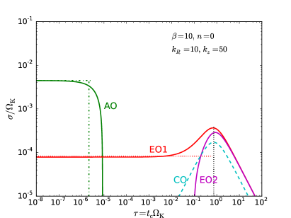
Figure 1.— Growth rate of the unstable mode versus thermal relaxation time. These solutions have been obtained without including vertical structure. The disk model parameters used are $(p,q,h,\gamma)=(-2,-1,0.05,1.4)$. The unstable growth rate $\sigma$ and the cooling time $\tau$ are non-dimensionalized in terms of $\Omega_{\rm K}$. The abbreviations used are: AO - Acoustic Overstability, EO1 - first radial epicyclic Overstability and EO2 - second radial epicyclic overstability

5.1. (Magneto-) Acoustic Overstability

In Figures 1, 2 and 3, we find an unstable mode, depicted by the solid green curve, that maintains an appreciable growth rate for very short cooling times and is swiftly damped beyond a critical time scale. This mode has an associated oscillatory part with a frequency, $\nu=Re[{\omega}]$, corresponding to that of acoustic waves in the disk. We, therefore, associate this mode with a rapidly oscillating overstable (magneto-)acoustic mode. The eigenvector of this acoustic overstable mode is shown in Figure 4(a).

The acoustic overstability is only present for very short cooling times. In order to capture the basic characteristic features of this mode, we reduce the dispersion relation (13) to the simpler form

$$\omega^{2}+it_{\rm c}F^{\rm A}_{3}\omega-F^{\rm A}_{4}=0\,,$$ (38)

with

$$F^{\rm A}_{3} =\gamma k^{2}c_{\rm i}^{2}\left(1+\frac{2}{\gamma\beta}\right)\,,$$ (39)

$$F^{\rm A}_{4} =k^{2}c_{\rm i}^{2}\left(1+\frac{2}{\beta}\right)+ik_{R}\frac{\partial c_{\rm i}^{2}}{\partial R}\,.$$ (40)

The coefficients $F^{\rm A}_{3}$ and $F^{\rm A}_{4}$ are reduced forms of the coeffcients $F_{3}$ and $F_{4}$ given by Equations (14) and (14). Here we have neglected terms containing shear and background pressure or density gradients from the coefficients in order to keep the analysis manageable yet retain the terms essential for instability. Notice that Equation (38) reduces to the quadratic form of the locally isothermal dispersion relation obtained when considering the limit, $t_{\rm c}\rightarrow 0$, in Equation (13). Substituting $\omega=\nu+i\sigma$, we can express the unstable growth rate as

$$\sigma\sim k_{R}\frac{\partial c_{\rm i}^{2}}{\partial R}\left[4k^{2}c_{\rm i}^{2}\left(1+\frac{2}{\gamma\beta}\right)\right]^{-1/2}\,.$$ (41)

The critical cooling time beyond which the overstable mode is rapidly damped is approximately

$$t_{\rm c,cr}\sim\sigma/F^{\rm A}_{3}\,.$$ (42)

The dash-dotted green colored lines in Figures 1 and 2 represent the numerical estimates for the growth rates and time scales obtained from Equations (41) and (42). Given the simplifications involved in obtaining these estimates, the agreement between the predictions for the growth rate and critical timescale from the analytical approximation and the numerical result is quite remarkable. In a magnetized disk, it is the fast magnetoacoustic waves that undergo overstable oscillations. The field itself has a very small effect on the growth rate and the tendency is to damp the amplification of the oscillations.

The thermal gradient is solely responsible for amplifying the otherwise stable acoustic waves. The thermal gradient adds to the restoring forces in such a way as to cause the amplitude of the near isothermal disturbances to grow exponentially with each oscillation.

5.2. Unstable Epicyclic Oscillations and the Convective Overstability

When the vertical structure of the disk is ignored, we find two overstable modes that are quite similar in character. Figure 1 shows two modes with peak growth rates around cooling time, $\tau\approx 1$. They have the exact same growth rates for $\tau>1$ but acquire different values for shorter cooling times, i.e., $\tau<1$. Interestingly, these modes are reminiscent of a recently discovered unstable mode that has been termed the convective overstability.

When considering disks without vertical structure, Klahr & Hubbard (2014); Lyra (2014) find that an unstable mode is present if the radial Brunt-Väisäla frequency of the system is negative, which corresponds to the familiar Schwarzschild criterion for convective instability to adiabatic perturbations. However, provided $k_{z}\gg k_{R}$, the overstable mode has significant growth rates for a small range of thermal relaxation times centred around, $\tau\approx 1$. For comparison, we plot in Figure 1 the growth rate of the convective overstable mode by solving the dispersion relation in (Lyra 2014, equation 25) for the same set of model parameters used here. It is apparent that there is a striking correspondence between the two nearly degenerate modes, that we see represented by the solid red and magenta curves in Figure 1, with the convective overstability represented by the dashed cyan curve. For ease of reference and to avoid confusion, we shall henceforth refer to the solid red curve as the first epicyclic mode and the solid magenta curve as the second epicyclic mode.Examination of the unstable eigenvalue and eigenvector, see Figures 4(a) and 4(b), reveals that these modes comprise of growing epicyclic oscillations. This is also the basic nature of the convective overstable modes as described by Klahr & Hubbard (2014); Lyra (2014).

Figure 1 also shows that the first epicyclic mode is present for shorter thermal relaxation times analogous to the acoustic overstable mode discussed in the previous section. In the locally isothermal limit, $t_{\rm c}\rightarrow 0$, the dispersion relation, Equation (13) becomes analytically tractable as it is in the locally adiabatic limit. When vertical structure is ignored, we find that two distinct overstable modes are present in this limit of infinitely fast thermal relaxation. One of them is the aforementioned overstable (magneto-)acoustic oscillations. The other mode is one in which the radial temperature gradient acts to drive epicyclic oscillations unstable. It is this other unstable mode that we observe as the first epicyclic mode in Figure 1.

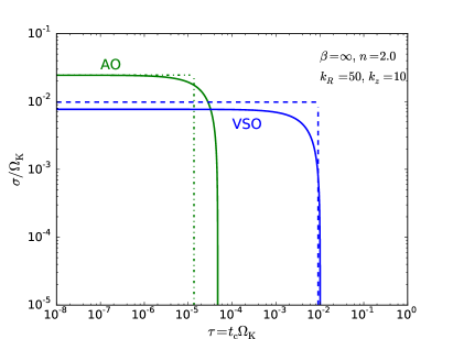
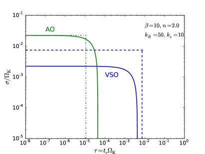
Figure 2.— Growth rate of the unstable mode versus thermal relaxation time. Inclusion of vertical gradients and in particular vertical shear gives rise to a different overstable mode. The disk model parameters used are $(p,q,h,\gamma)=(-2,-1,0.05,1.4)$. The unstable growth rate $\sigma$ and the cooling time $\tau$ are non-dimensionalized in terms of $\Omega_{\rm K}$. The abbreviations used are: AO - Acoustic Overstability, VSO - vertical shear overstability

We derive below characteristic growth rates and time scales associated with the first epicyclic mode. Performing a similar approximate analysis as in the previous subsection, we can derive analytical expressions that characterize the mode that persists at shorter cooling times. In the short cooling time limit, we obtain the reduced dispersion relation

$$\omega^{2}+it_{\rm c}F^{\rm E}_{5}\omega-F^{\rm E}_{6}=0,$$ (43)

with

$$F^{\rm E}_{5} =\gamma\mu^{2}(\kappa_{R}^{2}+N_{R}^{2})\left[1-\frac{ik_{R}}{k^{2}\left(1+2/\beta\right)}\frac{\partial\ln c_{\rm i}^{2}}{\partial R}\right],$$ (44)

$$F^{\rm E}_{6} =\mu^{2}\kappa_{R}^{2}\left[1-\frac{ik_{R}}{k^{2}\left(1+2/\beta\right)}\frac{\partial\ln c_{\rm i}^{2}}{\partial R}\right]\,,$$ (45)

where we have neglected the vertical background gradients. The growth rate is then approximately

$$\sigma\simeq-\frac{\kappa_{R}k_{R}k_{z}}{\sqrt{2}k^{3}\left(1+2/\beta\right)}\frac{\partial\ln c_{\rm i}^{2}}{\partial R}\,.$$ (46)

Were it not for the imaginary term containing the radial temperature gradient, this solution would simply represent stable epicyclic oscillations. The estimate for the growth rate (represented by the dotted red line) given by Equation (46) agrees remarkably well with the numerical result as seen in Figure 1. Continuing with the approximate analysis, we extract a characteristic timescale at which the growth rate declines rapidly

$$t_{\rm c,cr}\sim\sigma/F^{\rm E}_{5}.$$ (47)

Although derived assuming very small cooling times, the critical time expressed by Equation (47) coincides with the timescale for maximum growth provided that, $k_{R}\ll k_{z}$. While the growth rate does in fact fall beyond this critical time scale, it does not do so abruptly when an unstable radial entropy gradient is present.

The first epicyclic mode constitutes overstable epicyclic oscillations that are also referred to as acoustic-inertial oscillations. Isothermal perturbations in the presence of a radial temperature gradient add to the restoring forces as a fluid element is perturbed radially leading to overstability.

The second epicyclic overstable mode plotted in Figure 1 bears a much closer resemblance to the dashed cyan curve representing the convective overstability of Klahr & Hubbard (2014); Lyra (2014). Lyra (2014) performed a compressible local linear mode analysis of the convective overstability and derived analytical expressions for the characteristic growth rate and time scales. The dispersion relation given by Equation (13) in Section 3, reduces to Equation (17) in Lyra (2014) if we set all vertical gradients and the magnetic field to zero. However, the radial temperature gradient was omitted from the dispersion relation, Equation (19) in Lyra (2014) where it was argued that this term may be ignored as it is proportional to $1/R$. This exclusion cannot be rigorously justified and results in the divergent behaviour of the epicyclic modes remaining unseen. One possible argument to ignore the temperature gradient is to restrict the analysis to modes with $k_{R}=0$. However, this would go against the spirit of the short wave approximation upon which the entire local analysis is predicated. At the same time, it would also lead to growing modes that are essentially scale-independent. Ultimately, the justification for omitting any term ought to be consolidated by comparing against numerical solutions. Our results indicate that retaining the term containing the temperature gradient has a fundamental effect on the nature of the modes as illustrated by Figure 1 and should therefore not be discarded.

Despite these issues, the calculations by Lyra (2014) present the closest one can get to describing the second epicyclic mode analytically. Including the radial temperature gradient renders the dispersion relation intractable to analysis and it becomes difficult to extract even approximate expressions that characterize the unstable growth rate and time scales. Therefore, we rely on the analysis in Lyra (2014) and generalize it to include a toroidal magnetic field.

If we work in the anelastic approximation ($c_{\rm i}\rightarrow\infty$), as in Lyra (2014), the dispersion relation (13) assumes the form

$$\omega^{3}+i\varsigma\varepsilon\omega^{2}-\omega\left[\kappa_{R}^{2}+\bar{M}_{R}^{2}\right]-i\varsigma\mu^{2}\left[\kappa_{R}^{2}\varepsilon+\bar{L}_{R}^{2}\right]=0,$$ (48)

where we have made use of the definitions

$$\mu^{2} \equiv\frac{k_{z}^{2}}{k^{2}},$$ (49)

$$\varsigma \equiv\frac{1}{\gamma t_{\rm c}},$$ (50)

$$\varepsilon \equiv\frac{(1+2/\beta)}{(1+2/\gamma\beta)},$$ (51)

$$L_{R}^{2} \equiv-\frac{c_{\rm A}^{2}}{c_{\rm s}^{2}}\frac{1}{\rho_{0}}\frac{\partial P_{T}}{\partial R}\frac{\partial}{\partial R}\ln\left(\frac{B}{\rho}\right),$$ (52)

$$\bar{L}_{R}^{2} \equiv\frac{L_{R}^{2}}{(1+2/\gamma\beta)},$$ (53)

$$\bar{M}_{R}^{2} \equiv\frac{(N_{R}^{2}+L_{R}^{2})}{(1+2/\gamma\beta)}\,.$$ (54)

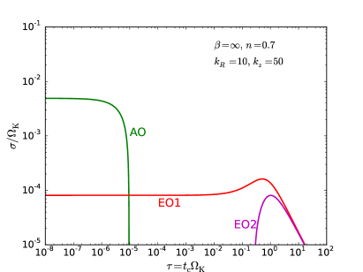
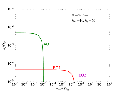
Figure 3.— Growth rate of the unstable mode versus thermal relaxation time. Illustration of the suppression of the epicyclic modes with increasing vertical shear. The disk model parameters used are $(p,q,h,\gamma)=(-2,-1,0.05,1.4)$. The unstable growth rate $\sigma$ and the cooling time $\tau$ are non-dimensionalized in terms of $\Omega_{\rm K}$. The abbreviations used are: AO - Acoustic Overstability, EO1 - first radial epicyclic Overstability and EO2 - second radial epicyclic overstability

In order to find approximate solutions to the dispersion relation (48), it is convenient to express $\omega$ explicitly as a complex variable, i.e., $\omega=\nu+i\sigma$, in the dispersion relation, Equation (48). The dispersion relation now splits it into a real and imaginary part both of which must equal to zero, respectively,

$$\nu^{2} - \mu^{2}\left[\kappa^{2}+\bar{M}_{R}^{2}\right]-3\sigma^{2}-2\sigma\varepsilon=0,$$ (55)

$$\sigma^{3} + \varsigma\varepsilon\sigma^{2}-\sigma\left[3\nu^{2}-\mu^{2}\bar{M}_{R}^{2}\right]$$ (56)

$$- \varsigma\left\{\nu^{2}-\mu^{2}\left[\varepsilon\kappa_{R}^{2}+\bar{L}_{R}^{2}\right]\right\}=0.$$

Substituting Equation (55) in Equation (56) yields

$$8\sigma^{3}+8\sigma^{2}\varsigma+2\sigma\left[\varsigma^{2}+\mu^{2}\left(\kappa^{2}+\bar{M}_{R}^{2}\right)\right]$$

$$+\varsigma\mu^{2}\left[\varepsilon\bar{N}_{R}^{2}+(\varepsilon-1)\bar{L}_{R}^{2}\right]=0.$$ (57)

We can obtain an approximate solution for this equation by noting that $\epsilon\simeq 1$ except for very small values of $\beta$ ($\varepsilon=1.23$ with $\beta=1$ and $\gamma=1.4$). Since $L_{R}^{2}\ll N_{R}^{2}$, except for very strong fields, in the limit of $\sigma\ll\varsigma$, we can neglect the cubic and quadratic terms, to obtain

$$\sigma\simeq-\frac{\varsigma\mu^{2}\bar{N}_{R}^{2}}{2\left\{\varsigma^{2}+\mu^{2}\left[\kappa^{2}+\bar{M}_{R}^{2}\right]\right\}}.$$ (58)

The criterion for this convective overstability is still effectively $N_{R}^{2}<0$ and the maximum growth rate

$$\sigma_{\rm max}=-\frac{|\mu|\bar{N}_{R}^{2}}{4\sqrt{\kappa^{2}+\bar{M}_{R}^{2}}}\,,$$ (59)

is achieved for

$$t_{\rm{c,max}}=\frac{1}{\sqrt{\gamma^{2}\mu^{2}\left[\kappa^{2}+\bar{M}_{R}^{2}\right]}}\,.$$ (60)

The effect of the magnetic field on the first epicyclic mode is to marginally dampen the growth rate. The growth rate of the second epicyclic mode appears slightly enhanced around $\tau\simeq 1$ for $\beta=10$. This is because the magnetic contribution to pressure support becomes larger for stronger fields and hence the effective radial gravitational acceleration increases. This causes the Brunt Väisäla frequency, in the manner we have defined it, to increase for stronger fields and consequently leads to a slight increase in growth rate.

(a) First Epicyclic Mode

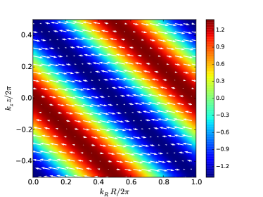
(b) Second Epicyclic Mode

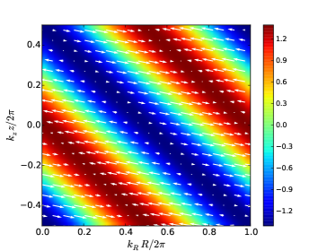
(c) Acoustic Mode

(d) Vertical Shear Mode

Figure 4.— Illustration of the unstable eigenvectors. The colored isocontours represent density perturbations and the arrows represent the flow in the $R-z$ plane. (a) and (b) represent the first and second epicyclic overstable mode respectively with $k_{R}H=10$ and $k_{z}H=50$ , (c) is the acoustic overstability with $k_{R}H=50$ and $k_{z}H=10$ and (d) the vertical shear overstable mode with $k_{R}H=50$ and $k_{z}H=10$. The disk model parameters used are $(p,q,h,\gamma,\beta)=(-2,-1,0.05,1.4,\infty)$.

5.3. Vertical Shear Overstability

When the vertical gradients of the background disk are taken into account, we identify another fundamental mode of instability, which is illustrated as the solid blue curve in Figure 2. As we shall see below, this mode can be attributed to the destabilizing effect of vertical shear in the disk.

Instability due to vertical shear has received much attention of late in connection with protoplanetary disks (Nelson et al., 2013; McNally & Pessah, 2014; Barker & Latter, 2015; Lin & Youdin, 2015). The destabilizing effect of vertical shear was first studied by Goldreich & Schubert (1967); Fricke (1968) and its role as a potential source of angular momentum transport in accretion disks was suggested by Urpin & Brandenburg (1998); Urpin (2003).

This unstable mode constitutes one of three overstable roots (along with the acoustic and acoustic-inertial modes) of the dispersion relation, Equation (13), in the locally isothermal limit, $t_{\rm c}\rightarrow 0$. Using indications obtained from the numerical solutions, we attempt to derive analytical approximations for the growth rate and critical timescale of the unstable mode due to vertical shear. By retaining only the terms essential to instability as done in the previous sections, we obtain a reduced dispersion relation in the short cooling time limit

$$\omega^{2}+it_{\rm c}F^{\rm V}_{5}\omega-F^{\rm V}_{6}=0,$$ (61)

with

$$F^{\rm V}_{5} =\frac{\gamma k_{R}^{2}M_{z}^{2}}{k^{2}(1+2/\beta)},$$ (62)

$$F^{\rm V}_{6} =\kappa_{R}^{2}\mu^{2}-\frac{i\kappa_{z}^{2}k_{R}}{k^{2}c_{\rm i}^{2}(1+2/\beta)}\frac{1}{\rho}\frac{\partial P_{\rm T}}{\partial z}.$$ (63)

Modes that are vertically elongated and radially narrow are known to tap the free energy in vertical shear more efficiently. For this reason, we have assumed $k_{R}\gg k_{z}$ in deriving the reduced form of the dispersion relation above. The unstable growth rate may then be approximated as

$$\sigma\sim\frac{\kappa_{z}^{2}k_{R}}{k^{2}c_{\rm i}^{2}(1+2/\beta)}\frac{1}{\sqrt{2}\kappa_{R}\mu\rho}\frac{\partial P_{\rm T}}{\partial z}\,,$$ (64)

and the critical cooling time beyond which the mode is rapidly damped is

$$t_{\rm c,cr}\sim\sigma/F^{\rm V}_{5}\,.$$ (65)

In the hydrodynamic limit, $\beta\rightarrow\infty$, and assuming vertical isothermality, the cooling time varies as

$$t_{\rm c,cr} \sim\frac{\sigma}{N_{z}^{2}}\propto\frac{1}{\gamma-1}\,,$$ (66)

Equation (66) is qualitatively similar to the critical cooling time estimate derived by Lin & Youdin (2015) in the radially local vertically global setting. The approximate estimates of the growth rate and critical cooling time have been over-plotted onto Figure 2. We find good agreement between the simplified estimates and the numerical values which implies that the basic ingredients of the instability are captured by the reduced analytical approximations. These modes are essentially overstable vertical epicyclic oscillations as is also suggested by the unstable eigenvector illustrated in Figure 4(d).

The unstable mode due to vertical shear that we have identified here has a different character to that which has been derived by linear analysis in previous studies. The unstable mode in Urpin & Brandenburg (1998); Urpin (2003) is a pure instability that is determined by the criterion

$$\kappa_{R}^{2}-\kappa_{z}^{2}\frac{k_{R}}{k_{z}}<0,$$ (67)

which is satisfied only if $k_{R}$ and $k_{z}$ are of opposite sign. The unstable mode due to vertical shear that we consider here under more general circumstances, is an overstable mode. In the isothermal limit $t_{c}\rightarrow 0$, the dispersion relation (13) reduces to Equation (32) derived in Nelson et al. (2013) if the radial background gradients are ignored and if we make the transformation $g\rightarrow g/2$, where $g$ is the vertical component of the gravitational acceleration. Note, however, that the crucial imaginary term in $F^{\rm V}_{6}$ is missing in Equation (32) of Nelson et al. (2013). We posit that this term is the real destabilizing source driving unstable motions in the disk. The fact that these unstable modes manifest as overstable oscillations is also borne out by the semi-global eigenmode calculations conducted in Nelson et al. (2013); McNally & Pessah (2014); Lin & Youdin (2015).

5.4. Coexistence of Epicyclic and Vertical Shear Modes

The numerical solutions in Section 5.2 were obtained without including the vertical gradients in the dispersion relation whereas those presented in Section 5.3 takes account of both radial and vertical gradients. The exclusion of vertical structure in Section 5.2 was performed with the intention to relate our results to previous studies where the analysis was similarly restricted to the horizontal plane. The question arises as to whether the overstable epicyclic modes occur in the presence of vertical stratification. Figure 2 does not contain the overstable radial epicyclic modes of Section 5.2 and seems to suggest that they are not present in a disk with vertical shear. We attempt below to analytically describe the observed trend by expanding the approximate analysis of the previous sections to include the terms relevant to the epicyclic and vertical shear modes in the reduced dispersion relation

$$\omega^{2}+i\gamma t_{\rm c}F^{EV}_{5}\omega-F^{EV}_{6}=0,$$ (68)

with

$$F^{EV}_{5} =\mu^{2}\kappa_{R}^{2}\left\{1-\frac{ik_{R}}{k^{2}\left(1+2/\beta\right)}\frac{\partial\ln c_{\rm i}^{2}}{\partial R}\right\},$$ (69)

$$F^{EV}_{6} =\left[\mu^{2}\kappa_{R}^{2}-\frac{i\kappa_{z}^{2}k_{R}}{k^{2}c_{\rm i}^{2}(1+2/\beta)}\frac{1}{\rho}\frac{\partial P_{\rm T}}{\partial z}\right]$$

$$\times\left\{1-\frac{ik_{R}}{k^{2}\left(1+2/\beta\right)}\frac{\partial\ln c_{\rm i}^{2}}{\partial R}\right\}.$$ (70)

The growth rate in this general situation can be approximated as

$$\sigma\simeq\left|\frac{\kappa_{R}k_{R}k_{z}}{\sqrt{2}k^{3}}\frac{\partial\ln c_{\rm i}^{2}}{\partial R}+\frac{\kappa_{z}^{2}k_{R}}{k^{2}c_{\rm i}^{2}}\frac{1}{\sqrt{2}\kappa_{R}\mu\rho}\frac{\partial P_{\rm T}}{\partial z}\right|$$ (71)

In the absence of vertical shear, the growth rate, given by Equation (71), reduces to that of the radial epicyclic mode. When vertical shear is present, Equation (71) suggests a competition of sorts between the radial epicyclic mode and vertical shear mode. For substantial vertical shear strengths and in particular for large radial wavenumbers, the overstable vertical shear mode alone survives. This is in accordance with the trend we observe from the numerical calculations. To illustrate the point, Figure 3 shows gradually weakening radial epicyclic modes as the vertical shear strength is increased. Our results suggest that the overstable radial epicyclic modes may not play a significant role in realistic accretion disks. Further studies of these modes in a global context will help to establish their relevance.

5.5. Scale Dependence of Unstable Modes

Our analysis thus far focussed on studying the unstable growthrates and critical timescales as a function of the thermal relaxation time and magnetic field strength. This was done for fixed representative values of the perturbation wavenumbers. Here, we examine the length scale preferences of the different modes identified in Figures 1 and 2. Figure 5 provides a graphical overview of the presence and strength of the unstable modes in wavenumber space obtained by numerically solving the general dispersion relation in Equation (13).

The acoustic overstable mode of Section 5.1 is seen to be dominant in the region of wavenumber space with $k_{R}\gg k_{z}$ in Figure 5(a). This is as one might expect since the disk has a non-zero radial temperature gradient that is coupled with the radial wavenumber. The modes representing radial epicyclic overstable oscillations of Section 5.2 show a preference for the $k_{z}\gg k_{R}$ region of wavenumber space. This aspect of the modes is in accord with the results of the local analysis by Lyra (2014). However, the two modes exhibit contrasting behaviors in the region $k_{R}H\simeq k_{z}H\leq 10$ of wavenumber space. The first epicyclic mode as represented by Figure 5(c) appears to be strongest for the above specified portion of wavenumber space. In contrast, the second epicyclic mode represented by Figure 5(b) is completely quenched in the said region. Note, however, that the inclusion of vertical structure in the computations quickly damp both these modes as pointed out in Section 5.3. A global or semi-global analysis can potentially shed more light on the relevance of the radial epicyclic modes. In Figure 5(d), we find that the vertical overstable mode dominates the $k_{R}\gg k_{z}$ region. A predisposition for that part of wavenumber space is also in accordance with expectation since destabilization by vertical shear occurs most effectively through radially narrow, vertically stretched perturbations (Nelson et al., 2013; McNally & Pessah, 2014; Barker & Latter, 2015; Lin & Youdin, 2015).

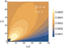
(a) First Epicyclic Mode

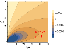
(b) Second Epicyclic Mode

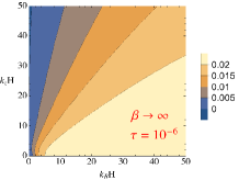
(c) Acoustic Mode

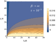
(d) Vertical Shear Mode

Figure 5.— The growth rates as a function of the perturbation wavenumbers for the disk model parameters $(p,q,h,\gamma)=(-1.5,-1,0.05,1.4)$. The coloured iso-contours represent the numerically computed values of the growth rates. (a) and (b) represent the first and second epicyclic overstable modes. (c) represents the acoustic overstable mode and (d) represents the vertical shear overstable mode. The preponderance of these modes stays the same for lower values of $\beta$.

6. Potential Relevance to Protoplanetary Disks

All the unstable modes that we find in the previous section have purely hydrodynamic manifestations and should therefore directly apply to protoplanetary disks. The applicability of the computations including a substantially strong toroidal magnetic field is not immediately obvious and requires some elaboration. Below we attempt to argue that our results including a magnetic field could be useful in addressing the question of axisymmetric stability within certain regimes of a disk.

While considering a purely toroidal magnetic field may seem a simplistic assumption, this provides important advantages that enable us to make connections to protoplanetary disks, where non-ideal effects play an important role: i) A purely toroidal field allows us to consider well-defined global equilibria for the disk. Both the global model, and its stability properties, can reach the hydrodynamic limit continuously. ii) The absence of a poloidal field eliminates the standard MRI, which nevertheless is expected to be significantly quenched in the bulk of the protoplanetary disk. iii) The fact that we can consider strong magnetic fields allows us to make connections with recent studies which suggest that fields with these characteristics can develop in certain intermediate regions within the disk, where ionization levels are very low.

The general consensus is that a sizeable extent of a protoplanetary disk constitutes an environment inhospitable to perfect coupling of magnetic fields to the disk gas. Yet, the standard accretion rates of $10^{-7}-10^{-9}M_{\odot}/$yr associated with such disks are most easily explained if one resorts to disk turbulence. The MRI is the most favored candidate by far, when it comes to explaining turbulent transport in disks. However, efficient operation of the MRI requires levels of ionization that are believed to be unattainable in significant portions of the disk. Several local and global studies have been undertaken to investigate MHD turbulence in the presence of some combination of the Ohmic, Hall and ambipolar effects. At intermediate densities, the Hall effect is believed to be the dominant non-ideal effect in a protoplanetary disk (Wardle, 1999).

Stratified shearing box simulations including all three non-ideal effects of ohmic diffusion, ambipolar diffusion and the Hall effect (Lesur et al., 2014; Simon et al., 2015) have lately challenged the magnetically inactive protoplanetary disk model. Lesur et al. (2014) have shown that if the initial magnetic field and angular velocity vector are aligned, the Hall effect, specifically the Hall-shear instability, leads to the generation of a strong azimuthal field that adds to pressure support. They speculate that this field geometry could possibly be found within the inner reaches of the disk, spanning between 1 and 10 AU. Local non-ideal MHD simulations by Bai (2014) also arrive at a similar picture. These studies find that the resulting field configurations generate laminar stresses that can account for the observed accretion rates, thereby, mitigating the need to appeal to hydrodynamic turbulence or even disk outflows. In a similar departure from a purely hydrostatic disk structure, Turner et al. (2014a) have appealed to magnetically supported atmospheres, with fields strong enough to alter the disk scale height, in order to explain the near-infrared excess seen emanating from disks around Herbig Ae/Be stars.

Diffusive non-ideal effects eventually smoothens out any gradients in the magnetic field distribution. Exact equilibrium disk models supporting non-uniform field configurations inclusive of non-ideal effects cannot therefore be derived. Unlike ohmic and ambipolar effects, the Hall effect is not diffusive but tends to rearrange field distributions. What is not yet clear, however, is whether the strong non-uniform field structures observed in simulations with Hall effect (Lesur et al., 2014; Bai, 2014; Simon et al., 2015) can sustain for extended periods. Under such circumstances, equilibrium disk models such as the one described in Section 2 may constitute useful, if not exact, representation of at least limited regions within the disk. The suitability of employing a localized version of such a disk model in a Hall dominated regime is aided by the fortuitous circumstance under which the linearized Hall term vanishes for axisymmetric perturbations. That is,

$$\nabla\times\eta_{\rm H}((\nabla\times\bm{B})\times\bm{B})=0\,,$$ (72)

where

$$\eta_{\rm H}=\frac{c}{4\pi n_{\rm e}e}$$ (73)

is the Hall coefficient taken to be uniform and $c$, $n_{\rm e}$, $e$, is the speed of light, the electron density, and the charge of the electron, respectively. Note also that $\bm{B}=(B_{0}+\delta b_{\phi})\bm{\hat{\phi}}$ represents the sum of the background and perturbed magnetic field in Equation (72). Therefore, even though our study does not explicitly account for non-ideal effects, our results may still shed light into the dynamics of disk regions where the Hall term dominates. While arguably rudimentary, this constitutes a first step towards an analytical understanding of the stability of disk environments suggested by the recent non-ideal MHD simulations.

7. Summary and Discussion

We have conducted a comprehensive axisymmetric local linear mode analysis of a stratified, differentially rotating disk threaded by a toroidal magnetic field in the ideal MHD limit. We employed a thermal relaxation model that allowed us to consider a wide range of physical conditions between (and including) the isothermal and adiabatic regimes. Our approach provides a framework to investigate the instabilities that can feed off of radial and vertical gradients in the dynamic and thermodynamic structure of the disk in a systematic way. This enables us to put into context previous studies that have addressed different aspects of this problem in isolation.

When thermal relaxation takes infinitely long, we find that a new criteria determines the local axisymmetric stability of disks in the presence of a purely toroidal field. For toroidal field configurations that contributes to pressure support, stronger fields act as a stabilizing influence. The new stability criterion we have derived reduces continuously to the Solberg-Høiland criteria in the hydrodynamic limit.

When thermal relaxation takes place on a finite timescale, the most important conclusions of this study can be summarized as follows. The mere presence of a background temperature gradient can give rise to overstable acoustic oscillations which dominate when thermal relaxation is rapid. A radial temperature gradient also gives rise to overstable radial epicyclic or acoustic-inertial oscillations. Combined with a negative radial entropy gradient, the growth rate of this epicyclic mode is amplified for longer cooling times. The negative radial entropy gradient also leads to the emergence of another overstable radial epicyclic mode that is similarly amplified by buoyancy but is present only for a narrow range of cooling times. The two epicyclic overstabilities have essentially the same eigenmode structure but differ with respect to growth rates for shorter cooling times. These epicyclic modes have been identified in a slightly different guise as the convective overstability. We posit that a spurious degeneracy due to the exclusion of the radial temperature gradient made its way into previous studies of the convective overstability. As a result, the dependence of the growth rate as a function of cooling time was not correctly captured in previous analysis. We believe that the true nature of these fundamental modes are best described by the results of our study. Strong vertical shear also leads to the development of overstable vertical epicyclic modes. These modes grow at an appreciable rate and are also present only for rather short cooling times. The critical value of the cooling time associated with the vertical shear overstability is longer than the corresponding time scale for the acoustic overstability. However, the growth rate of the overstable acoustic mode is larger than that of the mode due to vertical shear. In short, locally isothermal perturbations can generally give rise to unstable acoustic, radial epicyclic and vertical epicyclic oscillations. These three overstabilities are also present for finite albeit short values of cooling times and they are all quickly suppressed beyond a critical cooling times that is unique to each mode. Our results also indicate that the inclusion of both vertical and radial structure leads to the suppression of the radial epicyclic modes when vertical shear rates become substantial.

The thermal relaxation or cooling time has been taken as a free parameter in our analysis. The precise values or ranges of cooling time is a sensitive function of position, density, temperature, ionization degree, dust to gas ratio, magnetization and transport properties in the disk. Estimating the possible ranges of cooling times is a challenging enterprise and is beyond the scope of this work. Nonetheless, some amount of effort has been taken, to varying degrees of sophistication, in deriving theoretical estimates of cooling times in a disk in the context of the VSI. Both Nelson et al. (2013) and Lin & Youdin (2015) have attempted to analytically constrain the cooling times at different locations in the disk. They arrive at the general conclusion that the VSI should be active in the intermediate regions of the disk, generally between 5 AU and 50 AU. Our analysis reveals that the overstable acoustic modes have the strongest growth rates although they require much shorter cooling times. The overstable epicyclic modes grow with weaker growth rates although they can be present for a much wider range of cooling times. A thorough analysis of the extent and ranges of cooling times in a disk guided by observational constraints is thus warranted.

A global or semi-global analysis of all three overstabilities would certainly shed more light into the potential relevance of these modes. The non-linear evolution of these modes also merits further study.

References

- Acheson (1979) Acheson, D. J. 1979, Sol. Phys., 62, 23
- Armitage (2011) Armitage, P. J. 2011, ARA&A, 49, 195
- Avenhaus et al. (2014) Avenhaus, H., Quanz, S. P., Schmid, H. M., et al. 2014, ApJ, 781, 87
- Bai (2014) Bai, X.-N. 2014, ApJ, 791, 137
- Balbus (1995) Balbus, S. A. 1995, ApJ, 453, 380
- Balbus & Hawley (1991) Balbus, S. A., & Hawley, J. F. 1991, ApJ, 376, 214
- Balbus & Hawley (1992) —. 1992, ApJ, 400, 610
- Barker & Latter (2015) Barker, A. J., & Latter, H. N. 2015, MNRAS, 450, 21
- Christiaens et al. (2014) Christiaens, V., Casassus, S., Perez, S., van der Plas, G., & Ménard, F. 2014, ApJ, 785, L12
- Foglizzo & Tagger (1994) Foglizzo, T., & Tagger, M. 1994, A&A, 287, 297
- Foglizzo & Tagger (1995) —. 1995, A&A, 301, 293
- Fricke (1968) Fricke, K. 1968, ZAp, 68, 317
- Fukagawa et al. (2013) Fukagawa, M., Tsukagoshi, T., Momose, M., et al. 2013, PASJ, 65, L14
- Goldreich & Schubert (1967) Goldreich, P., & Schubert, G. 1967, ApJ, 150, 571
- Kato et al. (1998) Kato, S., Fukue, J., & Mineshige, S., eds. 1998, Black-hole accretion disks No. ISBN: 4876980535 (Kyoto University Press)
- Klahr & Hubbard (2014) Klahr, H., & Hubbard, A. 2014, ApJ, 788, 21
- Lesur et al. (2014) Lesur, G., Kunz, M. W., & Fromang, S. 2014, A&A, 566, A56
- Lesur & Ogilvie (2010) Lesur, G., & Ogilvie, G. I. 2010, MNRAS, 404, L64
- Lesur & Papaloizou (2010) Lesur, G., & Papaloizou, J. C. B. 2010, A&A, 513, A60
- Li et al. (2000) Li, H., Finn, J. M., Lovelace, R. V. E., & Colgate, S. A. 2000, ApJ, 533, 1023
- Lin & Papaloizou (1980) Lin, D. N. C., & Papaloizou, J. 1980, MNRAS, 191, 37
- Lin et al. (1993) Lin, D. N. C., Papaloizou, J. C. B., & Kley, W. 1993, ApJ, 416, 689
- Lin & Youdin (2015) Lin, M.-K., & Youdin, A. 2015, ArXiv e-prints, arXiv:1505.02163
- Lovelace et al. (1999) Lovelace, R. V. E., Li, H., Colgate, S. A., & Nelson, A. F. 1999, ApJ, 513, 805
- Lyra (2014) Lyra, W. 2014, ApJ, 789, 77
- Lyra & Lin (2013) Lyra, W., & Lin, M.-K. 2013, ApJ, 775, 17
- McNally & Pessah (2014) McNally, C. P., & Pessah, M. E. 2014, ArXiv e-prints, arXiv:1406.4864
- Muto et al. (2012) Muto, T., Grady, C. A., Hashimoto, J., et al. 2012, ApJ, 748, L22
- Nelson et al. (2013) Nelson, R. P., Gressel, O., & Umurhan, O. M. 2013, MNRAS, 435, 2610
- Newcomb (1961) Newcomb, W. A. 1961, Physics of Fluids, 4, 391
- Parker (1966) Parker, E. N. 1966, ApJ, 145, 811
- Parkin & Bicknell (2013a) Parkin, E. R., & Bicknell, G. V. 2013a, ApJ, 763, 99
- Parkin & Bicknell (2013b) —. 2013b, MNRAS, 435, 2281
- Pérez et al. (2014) Pérez, L. M., Isella, A., Carpenter, J. M., & Chandler, C. J. 2014, ApJ, 783, L13
- Pessah & Psaltis (2005) Pessah, M. E., & Psaltis, D. 2005, ApJ, 628, 879
- Ruden et al. (1988) Ruden, S. P., Papaloizou, J. C. B., & Lin, D. N. C. 1988, ApJ, 329, 739
- Rüdiger et al. (2002) Rüdiger, G., Arlt, R., & Shalybkov, D. 2002, A&A, 391, 781
- Ryu & Goodman (1992) Ryu, D., & Goodman, J. 1992, ApJ, 388, 438
- Schwarzschild (1958) Schwarzschild, M. 1958, Structure and evolution of the stars.
- Shu (1974) Shu, F. H. 1974, A&A, 33, 55
- Simon et al. (2015) Simon, J. B., Lesur, G., Kunz, M. W., & Armitage, P. J. 2015, ArXiv e-prints, arXiv:1508.00904
- Tassoul (2007) Tassoul, J.-L. 2007, Stellar Rotation
- Turner et al. (2014a) Turner, N. J., Benisty, M., Dullemond, C. P., & Hirose, S. 2014a, ApJ, 780, 42
- Turner et al. (2014b) Turner, N. J., Fromang, S., Gammie, C., et al. 2014b, Protostars and Planets VI, 411
- Urpin (2003) Urpin, V. 2003, A&A, 404, 397
- Urpin & Brandenburg (1998) Urpin, V., & Brandenburg, A. 1998, MNRAS, 294, 399
- Wardle (1999) Wardle, M. 1999, MNRAS, 307, 849