Red noise versus planetary interpretations in the microlensing event OGLE-2013-BLG-446

Abstract

For all exoplanet candidates, the reliability of a claimed detection needs to be assessed through a careful study of systematic errors in the data to minimize the false positives rate. We present a method to investigate such systematics in microlensing datasets using the microlensing event OGLE-2013-BLG-0446 as a case study. The event was observed from multiple sites around the world and its high magnification ($A_{\rm max}\sim 3000$) allowed us to investigate the effects of terrestrial and annual parallax. Real-time modeling of the event while it was still ongoing suggested the presence of an extremely low-mass companion ($\sim 3M_{\oplus}$) to the lensing star, leading to substantial follow-up coverage of the light curve. We test and compare different models for the light curve and conclude that the data do not favour the planetary interpretation when systematic errors are taken into account.

I. Introduction

For the past ten years, gravitational microlensing has been used to detect cool planets around G, K and M-stars in the Milky Way, allowing access to a planetary regime difficult to observe with the transit or radial velocity methods (i.e microlensing is sensitive to planets beyond the snowline). Due to the increased field of view of the OGLE-IV and MOA-II surveys, and the recently improved performance of follow-up teams, the number of planets detected by microlensing has gone up substantially (typically 10-20 planets detected per year and 33 published to date).

Another advantage of the microlensing method is that detection of planetary companions is possible over a larger mass-range [$\sim 1M_{\oplus},\sim 13M_{J}$], including brown dwarfs, if the projected orbital radius $s$ is in the range 0.6-1.6 $R_{E}$ (i.e the classical ”lensing zone”). Thanks to better photometric coverage of light curves, recent studies have advanced claims about the detection of small planets Bennett et al. (2014). However, smaller mass-ratios tend to produce smaller deviations from a single lens model most of the time. Failing to account for photometric systematics can potentially lead to false detections. The analysis of photometric systematics has been important in transit searches and has substantially improved the reliability of detections Kovács et al. (2005); Smith et al. (2012). This point is too often neglected by the microlensing community.

In this work, we present an extensive study of photometric systematics for the case of OGLE-2013-BLG-0446 and we compare the significance when different microlensing models are considered. Section II presents a summary of the observations of microlensing event OGLE-2013-BLG-0446 from multiple sites around the world. We present our modeling process in Section III and conduct a study of systematics in the data in Section IV. We present our conclusions in Section V.

II. Observations

Microlensing event OGLE-2013-BLG-0446 ($\alpha=18^{h}06^{m}56^{s}.18$, $\delta=-31^{\circ}39^{\prime}27^{\prime\prime}.2$ (J2000.0); $l=0.049^{\circ}$, $b=-5.344^{\circ}$) was discovered on the $6^{th}$ April 2013 by the Optical Gravitational Lens Experiment (OGLE) Early Warning System Udalski (2003b) and later alerted by the Microlensing Observations in Astrophysics (MOA) Bond et al. (2001). Observations obtained on the rising part of the light curve indicated that this event could be highly magnified and might therefore be highly sensitive to planets Griest & Safizadeh (1998); Yee et al. (2009); Gould et al. (2009). Follow-up teams, such as $\mu$FUN Gould et al. (2006), PLANET Beaulieu et al. (2006), RoboNet Tsapras et al. (2009) and MiNDSTEp Dominik et al. (2008), then began observations a few days before the peak of the event. The peak magnification was $\sim$ 3000 and the peak was densely sampled from different observatories.

The various teams used difference image analysis (DIA) to obtain photometry: $\mu$FUN used pySIS Albrow et al. (2009), with the exception of the Auckland data, which were re-reduced using DanDIA Bramich (2008); Bramich et al. (2013). DanDIA was also used to reduce the RoboNet and the Danish datasets. PLANET data were reduced online with the WISIS pipeline, and final data sets were prepared using pySIS. OGLE Udalski & Szymański (2015) and MOA Bond et al. (2001) used their own DIA code to reduce their frames. All other data sets were reduced using pySIS.

A total of 2955 data points from 16 telescopes were used for our analysis, after problematic data points were masked. A summary of each data set is available in Table 1.

Name	Collaboration	Location	Aperture(m)	Filter	Code	$N_{data}$	Longitude($\deg$)	Latitude($\deg$)
$\rm{OGLE\_I}$	OGLE	Chile	1.3	I	Woźniak	463	289.307	-29.015
$\rm{OGLE\_V}$	OGLE	Chile	1.3	V	Woźniak	24	289.307	-29.015
$\rm{Canopus\_I}$	PLANET	Tasmania	1.0	I	pySIS	132	147.433	-42.848
$\rm{Auckland\_R}$	$\mu$FUN	New Zealand	0.4	R	DanDIA	107	147.777	-36.906
$\rm{LSCB\_i}$	RoboNet	Chile	1.0	SDSS-i	DanDIA	378	289.195	-30.167
$\rm{LSCA\_i}$	RoboNet	Chile	1.0	SDSS-i	DanDIA	385	289.195	-30.167
$\rm{CPTA\_i}$	RoboNet	South Africa	1.0	SDSS-i	DanDIA	22	20.810	-32.347
$\rm{CTIO\_I}$	$\mu$FUN	Chile	1.3	I	pySIS	112	289.196	-30.169
$\rm{CTIO\_V}$	$\mu$FUN	Chile	1.3	V	pySIS	13	289.196	-30.169
$\rm{Danish\_z}$	MiNDSTEp	Chile	1.5	i+z	DanDIA	452	289.261	-29.255
$\rm{MOA\_Red}$	MOA	New Zealand	1.8	Red	Bond	454	170.464	-43.987
$\rm{Possum\_N}$	$\mu$FUN	New Zealand	0.4	N	pySIS	244	177.856	-38.623
$\rm{Salerno\_I}$	MiNDSTEp	Italy	0.4	I	pySIS	20	14.799	40.772
$\rm{Turitea\_R}$	$\mu$FUN	New Zealand	0.4	R	pySIS	31	175.630	-40.353
$\rm{Weizmann\_I}$	$\mu$FUN	Israel	0.4	I	pySIS	60	34.811	31.908
$\rm{SAAO\_I}$	PLANET	South Africa	1.0	I	pySIS	58	20.789	-32.374

Table 1Summary of observations. N is unfiltered dataset.

III. Modeling

III.1. Source properties

This event shows clear signs of finite-source effects and the limb darkening coefficients must be evaluated for each data set. We first consider a point-source point-lens model (PSPL) Paczyński (1986). The PSPL model allows the estimation of the source and blended fluxes in the V and I passbands for the calibrated OGLE photometry, leading to a good approximation for the V and I magnitudes of the source, which in turn allows us to derive a rough color for the source. We found $(I,(V-I))_{PSPL}=(19.07,1.48)$. Using the Interstellar Extinction Calculator on the OGLE website based on Nataf et al. (2013), we found that the Galactic Bulge true distance modulus for this line of sight is $\mu=14.578\pm 0.326$ mag ($d_{\rm{Bulge}}=8.2\pm 1.2$ kpc), the I band extinction is $A_{I}=0.804$ mag and the reddening is $E(V-I)=0.683\pm 0.036$ mag, leading to $R_{I}={A_{I}}/{E(V-I)}=1.177$, lower than the standard value of 1.5. This low extinction is known as the anomalous extinction law towards the Galactic Bulge, see Udalski (2003a). We derive the source properties as follows:

• Assuming that the source suffers the same extinction as the Red Giant Clump (i.e the source is at the same distance), we have $M_{I}=19.07-0.804-14.578=3.7$ mag, so the source star is most likely a main sequence star. We adopt $\log g\sim 4.5$.

• We derive its effective temperature using the dereddened color-magnitude relation for dwarfs and subgiants (relation (3) in Casagrande et al. (2010)) with solar metallicity.

• From Claret (2000) and using $\log g\sim 4.5$, we are able to find the linear limb-darkening coefficients $u_{\lambda}$ Milne (1921) for each filter. Following Albrow et al. (1999); Yoo et al. (2004), we use the transformation :

  $$\Gamma_{\lambda}={{2u_{\lambda}}\over{3-u_{\lambda}}}$$ (1)

These calculations form the starting point for an iterative fit of the FSPL (finite source point lens) model, together with error-bar rescaling as described in Section III.3. Our best FSPL model converges to source magnitude and color $(I,(V-I))=(19.00,1.49)$. Correcting for extinction and reddening we have $(I_{o},(V-I)_{o})=(18.20,0.81)$. The corresponding effective temperature of the source is $T_{\rm{eff}}\sim 5400~{}K$, leading to $\Gamma_{V}=0.63~{}(u_{V}=0.72)$, $\Gamma_{R}=0.55~{}(u_{R}=0.65)$ and $\Gamma_{I}=0.46~{}(u_{I}=0.56)$ for $\log g\sim 4.5$. Note that we also use $\Gamma_{I}=0.46$ for the RoboNet telescopes (SDSS-i filter). Finally, given the dereddened magnitude and colour of the source from our best FSPL model, we are able to estimate the angular source star radius $\theta_{*}$ using Kervella & Fouqué (2008):

$$\log_{10}(\theta_{*})=3.1982+0.4895(V-I)_{o}-0.0657(V-I)_{o}^{2}-0.2I_{o}$$ (2)

The uncertainty of this relation is 0.0238. The errors on our magnitude estimates are $(\Delta I,\Delta V)=(0.02,0.02)$ mag. Assuming a conservative estimate of the error on $A_{I}$ (0.1 mag) and using standard error propagation gives 9% precision: $\theta_{*}=0.82\pm 0.07~{}\mu as$. With the adopted source distance (8.234 kpc), the source star radius is $R_{*}=1.4\pm 0.3~{}R_{\odot}$. Therefore the source is a G6 or K0 star Bessell & Brett (1988).

III.2. Single lens model

The PSPL model is described by the standard single-lens parameters : $t_{E}$ the Einstein crossing time, $u_{o}$ the minimum impact parameter and $t_{o}$, the time of this minimum. The normalized angular source radius $\rho={\theta_{*}}/{\theta_{E}}$ Nemiroff & Wickramasinghe (1994); Witt & Mao (1994); Gould (1994); Bennett & Rhie (1996); Vermaak (2000), where $\theta_{E}$ is the angular Einstein ring radius, is included in the model along with the previous parameters to take into account finite-source effects close to the magnification peak. We used the method described in Yoo et al. (2004) to take into account the change in magnification due to the extended source. The FSPL model significantly improves the fit (see Table 3). The best FSPL model is shown in Figure 1.

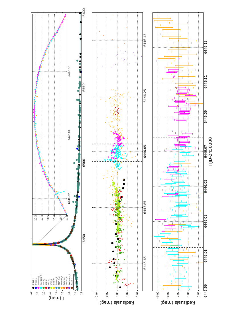
Figure 1.— Light curve of OGLE-2013-BLG-0446 with our best FSPL model. The top panel shows the full 2013 light curve with a maximum magnification at $HJD-2450000\sim 6446.0$ d. The insert on the right is a zoom of the peak. The pink model light curve is for $\Gamma_{I}=0.46$ and the orange dashed model light curve is for $\Gamma_{V}=0.63$. The cyan model for the R band is not shown for clarity. The cyan arrow indicates the position of the possible planetary anomaly. The middle panel shows residuals of the FSPL model close to the peak. The radius of each point is proportional to the inverse square of the error bar (bigger points have smaller error bars). The bottom panel is a closer view of the possible anomaly. For the bottom two panels, vertical dashed black lines indicate the time window corresponding to the insert in the top figure.

Using the value of $\rho$ from the FSPL model, we are able to estimate the angular radius of the Einstein ring $\theta_{E}={\theta_{*}}/{\rho}=1.57\pm 0.1$ mas and the lens-source proper motion $\mu={\theta_{E}}/{t_{E}}=7.4\pm 0.7~{}\rm{mas~{}yr}^{-1}$.

III.3. Treatment of photometric uncertainties and rejection of outliers

Because of the diversity of observatories and reduction pipelines used in microlensing, photometric uncertainties need careful rescaling to accurately represent the real dispersion of each data set. This is an important preliminary step in modeling the event. Following Bachelet et al. (2012b); Miyake et al. (2012); Yee et al. (2013), we rescale the uncertainties using :

$$e^{\prime}_{i}=\sqrt{(fe_{i})^{2}+e_{min}^{2}}$$ (3)

where $e_{i}$ are the original magnitude uncertainties, $f$ is the rescaling parameter for low magnification levels, $e_{min}$ is a minimal uncertainty to reproduce the practical limitations of photometry and $e^{\prime}_{i}$ are the adjusted magnitude uncertainties. The classical rescaling method is to adjust $f$ and $e_{min}$ to force ${\chi^{2}}/{dof}$ to be unity.

In this paper, we follow an alternative method of first adjusting $f$ and $e_{min}$ to force the residuals, normalized by $e^{\prime}_{i}$, to follow a Gaussian distribution around the model. If possible, we also aim to obtain a ${\chi^{2}}/{dof}\sim 1$. Note that these two methods lead to the same results, except for the OGLE_I dataset. For OGLE_I, the distribution without rescaling shows some data points with large residuals. This is not surprising because the OGLE_I data set covers the entire light curve with a large number of points, especially the faint baseline magnitude ($I\sim 17.8$), with a constant exposure time in order of 100 s. Inspection of the OGLE_I light curve reveals that the uncertainties during high magnification are underestimated, so we adjust the $e_{min}$ parameter. We tried to force ${\chi^{2}}/{dof}\sim 1$ for this dataset, but this generated large uncertainties for the low magnification part (i.e. the baseline) leading to a non-Gaussian distribution (lots of normalised residuals too close to the mean).

We finally checked isolated points far away from this Gaussian distribution, and reject as outliers ($>7\sigma$) two data points in the Auckland_R dataset. The rescaling coefficients are presented in Table 2.

Name	$N_{data}$	$\Gamma_{\lambda}$	f	$e_{min}$
$\rm{OGLE\_I}$	463	0.46	1.0	0.002
$\rm{OGLE\_V}$	24	0.63	10.25	0.0
$\rm{Canopus\_I}$	132	0.46	3.0	0.005
$\rm{Auckland\_R}$	107	0.55	1.75	0.005
$\rm{LSCB\_i}$	378	0.46	1.4	0.003
$\rm{LSCA\_i}$	385	0.46	2.0	0.007
$\rm{CPTA\_i}$	22	0.46	1.19	0.0
$\rm{CTIO\_I}$	112	0.46	1.5	0.004
$\rm{CTIO\_V}$	13	0.63	1.0	0.0
$\rm{Danish\_z}$	452	0.46	5.0	0.008
$\rm{MOA\_Red}$	454	0.51	1.0	0.0
$\rm{Possum\_N}$	244	0.63	1.5	0.008
$\rm{Salerno\_I}$	20	0.46	3.91	0.0
$\rm{Turitea\_R}$	31	0.55	1.0	0.005
$\rm{Weizmann\_I}$	60	0.46	3.2	0.01
$\rm{SAAO\_I}$	58	0.46	2.57	0.008

Table 2 Limg darkening and error bar rescaling coefficients used in this paper.

III.4. Annual and terrestrial parallaxes

We looked for second-order effects in the light curve. First, the relatively long Einstein-ring crossing-time ($t_{E}\sim 80$ days) should allow the measurement of the displacement of the line-of-sight towards the target due to the Earth’s rotation around the Sun. This annual parallax Gould & Loeb (1992); Gould (2000); Smith et al. (2003); Gould (2004); Skowron et al. (2011) is described by the vector $\pi_{E,a}={AU}/{\widetilde{r_{E}}}=(\pi_{EN},\pi_{EE})$, where $\widetilde{r_{E}}$ is the angular radius of the Einstein ring of the lens projected onto the observer plane and $\pi_{EN}$ and $\pi_{EE}$ are the components of this vector in the North and East directions respectively. In practice, the introduction of this parameter slightly changes the value of the impact parameter and $\tau={(t-t_{o})}/{t_{E}}$. Strong modifications of the light curve can be seen far from the peak of the event, i.e in the wings of the light curve, with few changes around the peak, see for example Smith et al. (2003). To model this effect, the constant $t_{o,par}$ Skowron et al. (2011) is added to give an invariant reference time for each model. We choose $t_{o,par}=2456446.0$ HJD for our models.

Since this event is so highly magnified, it should also be possible to measure the terrestrial parallax. Hardy & Walker (1995) first introduced the idea that for an ’Extreme Microlensing Event’ (EME), the difference in longitudes of observatories should result in light curves where tiny changes in the line-of-sight towards the target become apparent, allowing a measurement of the Einstein ring Holz & Wald (1996); Gould (1997); Dong et al. (2007). Again, this effect is described by the parallax vector $\pi_{E,t}={AU}/{r_{\oplus}}({\Delta t_{o}}/{t_{E}},\Delta U_{o})$, where $r_{\oplus}$ is the Earth radius. Gould & Yee (2013) estimated that the condition $\rho\widetilde{r_{E}}\leq 50r_{\oplus}$ is required to expect a measurable difference in terms of magnification. This condition leads to $\pi_{E}>0.24$ for this event by using an approximate value for the normalized source star radius $\rho\sim 5\times 10^{-4}$. A summary of longitudes and latitudes of the observatories is in Table 1 and results are summarized in Table 3.

Note that we also compute the annual parallax model for a positive impact parameter ($u_{0}>0$) and found no significant difference with the model reported in the Table 3. This is the $u_{0}$ degeneracy described in the literature Smith et al. (2003); Gould (2004); Skowron et al. (2011). For the terrestrial parallax, a positive impact parameter leads to a better fit ($\Delta\chi^{2}\sim 60$) for equivalent $\pi_{EN}$ and $\pi_{EE}$ values , which is a similar result to Yee et al. (2009).

III.5. Binary model

At the end of the 2013 observing season, several planetary models circulated (private communication) indicating the presence of the smallest microlensing planet ever detected ($q\sim 2\times 10^{-5}$). In order to investigate these claims of the existence of a very low-mass ratio planetary companion to the primary lens, and to exclude the possibility of a false alarm, we used a finite-source binary lens model (FSBL) with three extra parameters: the projected separation (normalized by $\theta_{E}$) between the two bodies $s$ , the mass ratio $q$ using the convention described in Bachelet et al. (2012a) (the most massive component on the left) and $\alpha$ the source trajectory angle measured from the line joining the two components (counterclockwise angle). We first used a grid search and we finally explore minima with a full Markov-Chain Monte Carlo algorithm (MCMC). Please see for example Dong et al. (2009) or Bachelet et al. (2012a) for more details. We find two local minima which correspond to the known theoretical degeneracy $s\Leftrightarrow s^{-1}$. We only explore the ’wide’ solution, which gives the best grid-search $\chi^{2}$, for three reasons. First, as explained in the next section, the reliability of the planetary model is not clear. Second, we expect a strong degeneracy in terms of $s\Leftrightarrow s^{-1}$, so models should converge to solutions with similar shapes for the central caustic and therefore similar residuals. Finally, due to the really small value of $\rho$, modeling this event is very time consuming. We present our results in Table 3, our best caustic-crossing geometry in Figure 2 and redisuals to the FSPL model for data sets covering the magnification peak are plotted in Figure  3.

Parameters	FSPL	FSPL+Annual parallax	FSPL+Terrestrial parallax	Wide planetary (FSBL)
$t_{o}$(HJD)	$6446.04790\pm 3~{}10^{-5}$	$6446.04678\pm 3~{}10^{-5}$	$6446.04681\pm 3~{}10^{-5}$	$6446.04659\pm 3~{}10^{-5}$
$U_{o}$($\theta_{E}$)	$-4.21~{}10^{-4}\pm 7~{}10^{-6}$	$-4.02~{}10^{-4}\pm 8~{}10^{-6}$	$-4.22~{}10^{-4}\pm 8~{}10^{-6}$	$-4.31~{}10^{-4}\pm 5~{}10^{-6}$
$t_{E}$(days)	$76.9\pm 1.3$	$80.4\pm 1.5$	$76.5\pm 1.4$	$76.0\pm 0.7$
$\rho$($\theta_{E}$)	$5.22~{}10^{-4}\pm 9~{}10^{-6}$	$4.99~{}10^{-4}\pm 1~{}10^{-5}$	$5.24~{}10^{-4}\pm 9~{}10^{-6}$	$5.31~{}10^{-4}\pm 5~{}10^{-6}$
$I_{s}$(mag)	$19.00\pm 0.02$	$19.05\pm 0.02$	$19.00\pm 0.02$	$18.99\pm 0.01$
$V_{s}$(mag)	$20.49\pm 0.02$	$20.54\pm 0.02$	$20.49\pm 0.02$	$20.48\pm 0.01$
$I_{b}$(mag)	$18.21\pm 0.01$	$18.18\pm 0.01$	$18.21\pm 0.01$	$18.22\pm 0.01$
$V_{b}$(mag)	$22.72\pm 0.11$	$22.35\pm 0.11$	$22.76\pm 0.13$	$22.85\pm 0.07$
$\Pi_{EN}$		$0.37\pm 0.15$	$0.07\pm 0.02$
$\Pi_{EE}$		$0.27\pm 0.005$	$0.01\pm 0.02$
$s$($\theta_{E}$)				$1.68\pm 0.05$
$q$				$3.1~{}10^{-5}\pm 2~{}10^{-6}$
$\alpha$(rad)				$-2.39\pm 0.02$
$\chi^{2}$	3900.781	3839.267	3877.241	3551.217

Table 3Model parameters.

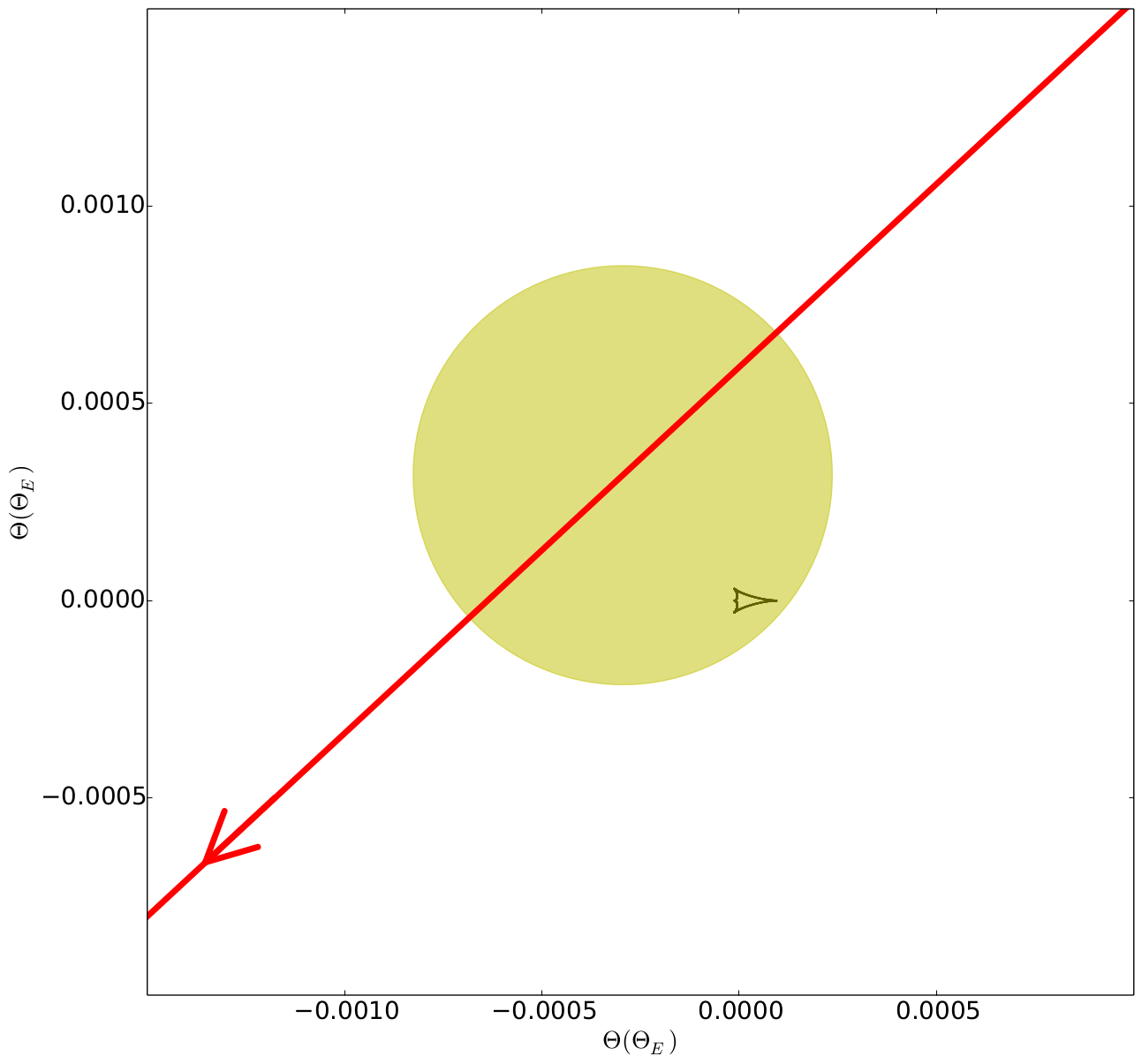
Figure 2.— Lens geometry for our best fit planetary model. The yellow disc represents the source, the red line indicates the source trajectory and the black closed curve represents the central caustic. The caustic signature in the light curve is highly ’diluted’ by the relatively large source star.

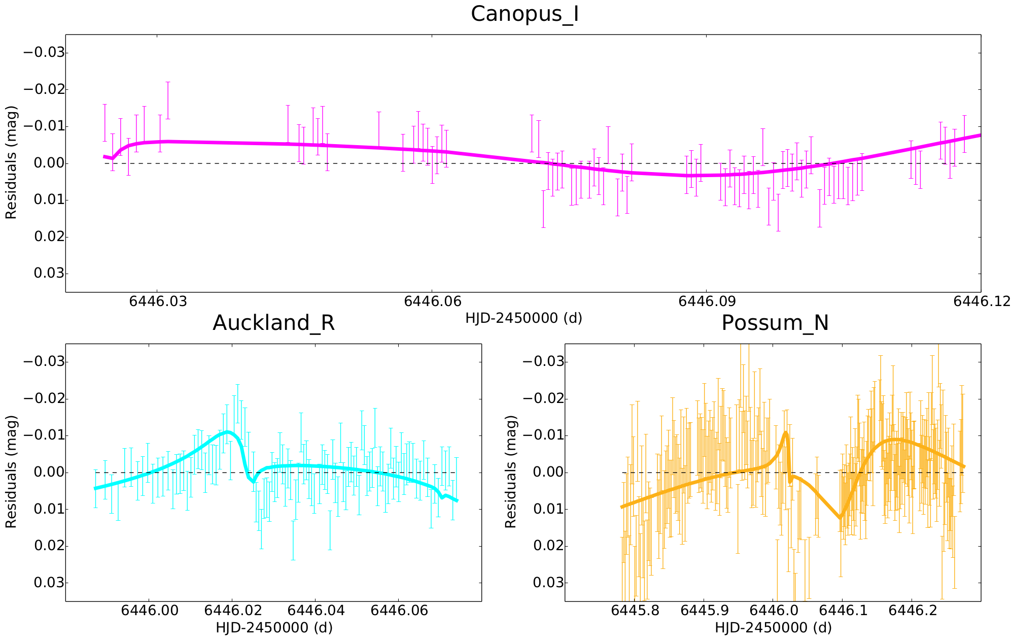
Figure 3.— FSPL residuals close to the peak. The curves represent the best planetary model.

IV. Study of systematic trends in the photometry

IV.1. Generality and method

Our best planetary model claims the detection of smooth deviations in the light curve away from the FSPL model at a peak-to-peak level of $\leq 1\%$, which is supposedly caused by the source passing over the central planetary caustic. It is well known to photometrists, however, that from ground-based telescopes the photometric precision at this level can be affected by systematic trends (or red noise) in the data.

In the early days of planet hunting using the transit method, researchers were confounded as to why they were not finding as many planets as predicted. The predictions were of course based on simulated light curves taking into account stochastic noise from the photons (sky and star) and the CCD, but ignoring the effects of sub-optimal data calibration/reduction that introduce correlated noise (e.g. Mallén-Ornelas et al. (2003) and Pepper & Gaudi (2005)). It was soon realised that transit detection thresholds were severely affected by systematic trends in the light curves Pont et al. (2006); Aigrain & Pont (2007) with the knock-on effect of reducing the predicted planetary yield of a transit survey, and at least partially explaining the unexpectedly low rate of transiting planet discoveries. The microlensing planet hunters face a similar problem for detecting low-amplitude ($\lesssim$1%) planetary deviations in microlensing light curves, especially when no “sharp” light curve features, caused by caustic crossing events, are predicted/observed. However, the microlensing community is now aiming for really low amplitude signal detection which requires extra care in the treatment of systematic errors Yee et al. (2013).

Systematic trends in light curve data can be caused by an imperfect calibration of the raw data and sub-optimal extraction of the photometry. For instance, on the calibration side, flat fielding errors which vary as a function of detector coordinates can induce correlated errors in the photometry as the telescope pointing drifts slightly during a set of time-series exposures. On the software side, systematic errors in the photometry can be caused by errors in the PSF model used during PSF fitting for example. Also the airmass and transparency variations in the datasets should be modeled in the DIA procedure by the photometric scale factor. However, there is no garantee that the DIA modeling is perfect and this can create systematics trends in the data. As recently discussed by Bramich et al. (2015), an error $\epsilon_{p}$ in the estimate of the photometric scale factor leads directly to an error $\epsilon_{p}$ in the photometry. For example, the passage of clouds during data acquisition can create inhomogeneous atmospheric transparency in the frames and lead to a spatially varying photometric scale factor. The estimation of the photometric scale factor in DIA by using a ’mean’ value for the whole frame will produce different systematic trends for each star in the field of view. In practice, the expected error $\epsilon_{p}$ is order of a few %, which is non-critical for the majority of microlensing deviations, but can easily imitate the smallest such as in OGLE-2013-BLG-0446.

Obtaining a photon-noise limited data calibration and photometric extraction is not always feasible. Therefore complementary techniques have been developed to perform a relative calibration of the ensemble photometry after the data reduction (i.e. a post-calibration). These techniques can be divided into two broad groups; namely, detrending methods that do not use any a priori knowledge about the data acquisition or instrumental set up (e.g. Tamuz et al. (2005)), and photometric modelling methods that attempt to model the systematic trends based on the survey/instrumental properties (e.g. Honeycutt (1992); Padmanabhan et al. (2008); Regnault et al. (2009)). Each data point is associated with a unique object and a unique image (epoch), and carries associated metadata such as magnitude uncertainty, airmass, $(x,y)$ detector coordinates, PSF FWHM, etc. To investigate the systematic trends in the photometry, we firstly identified a set of object/image properties which we suspected of having influenced the quality of the data reduction. For each of these quantities, we defined a binning that covers the full range of values with an appropriate bin size. For each bin, we introduced an unknown magnitude offset to be determined, the purpose of which is to model the mean difference of the photometric measurements within the corresponding bin from the rest of the photometric measurements. We constructed our photometric model by adopting the unknown true instrumental magnitude of each object and the magnitude offsets as parameters. Since the model is linear, the best-fit parameter values corresponding to the minimum in $\chi^{2}$ may be solved for directly (and in a single step using some matrix algebra - see Bramich & Freudling 2012). Iteration is of course mandatory to remove variable stars and strong outliers from the photometric data set. A valid criticism of this method is that the systematic trends are derived from the constant stars but then applied to all stars including the variable stars (the microlensing event in our case). The question arises as to whether this approach is consistent? To argue our case, we are limited to showing that the method works in practice and we direct the reader to Figure 1 of Kains (2015) where RR Lyrae light curves in M68 are much improved by this self-calibration method. We used this method to analyse systematic trends in three data sets. They are listed below.

IV.2. LSCA_i and LSCB_i : the twins paradox

We opted to employ the above methodology in order to investigate and understand the systematic trends in the LSCB_i and LSCA_i data sets using the algorithms described in Bramich & Freudling (2012). These telescopes are twins : both are LCOGT 1m telescope clones, both supporting Kodak SBIG STX-16803 CCDs at the time of these observations. SDSS-i prescription filters manufactured at the same time were use to observe OGLE-2013-BLG-0446 during the same period of observation, though not precisely synchronously.

We first chose to study LSCB_i because this telescope most strongly favors the planetary model ($\Delta\chi^{2}\sim 128.3$, see Table 6). For LSCB_i, the DanDIA pipeline extracted 4272 light curves from the images in the LSCB_i data set, each with 378 data points (or epochs), which yields a total of 1614816 photometric data points. We investigated each object/image property in turn using the above method, and determined the peak-to-peak amplitude of the magnitude offsets in each case. The results are reported in Table  4. The trends in the photometry were found to be at the sub-mmag level for all correlating properties except for the epoch (2.0 mmag). The magnitude offsets determined for each epoch (or image) serve to correct for any errors in the fitted values of the photometric scale factors during DIA. The magnitude offsets as a function of detector coordinates (commonly referred to as an illumination correction - e.g. Coccato et al. (2014)) were modelled using a two-dimensional cubic surface (as opposed to the binning previously described) so as to better capture the large-scale errors in the flat-fielding. The peak-to-peak amplitude of the cubic surface over the full detector area was found to be $\sim$60 mmag, but since the LSCB_i observations only drifted by $\sim$50 pixels in each coordinate, we found that the magnitude offsets applicable to the OGLE-2013-BLG-446 light curve have a peak-to-peak amplitude of only $\sim$0.2 mmag. This can be seen in Figure  4. The overall level of systematic trends in the LSCB_i data set for OGLE-2013-BLG-446 is $\sim$2.0mmag. To conclude, this analysis reveals that the illumination correction is not sufficient to explain the observed systematics.

Correlating Quantity	Possible Underlying Cause	Peak-To-Peak Amplitude(mmag)
		LSCA_i	LSCB_i	Auckland_R
Exposure time	CCD non-linearities	20	0.3	60
Airmass	Varying extinction	22	0.8	40
PSF FWHM	Varying seeing disk	25	0.4	28
Photometric scale factor	Reduction quality at different transparencies	20	0.2	40
Epoch	Errors in photometric scale factor	60	2.0	120
Detector coordinates	Flat-field errors	10	0.2	*
Background	Reduction quality	27	0.5	45

Table 4The peak-to-peak amplitude of the magnitude offsets for each object/image property that we investigated for causing systematic trends in the photometry for the LSCB_i, LSCA_i and Auckland_R. data sets We also list a possible underlying cause for any systematic trends that are found as a function of the corresponding object/image property.

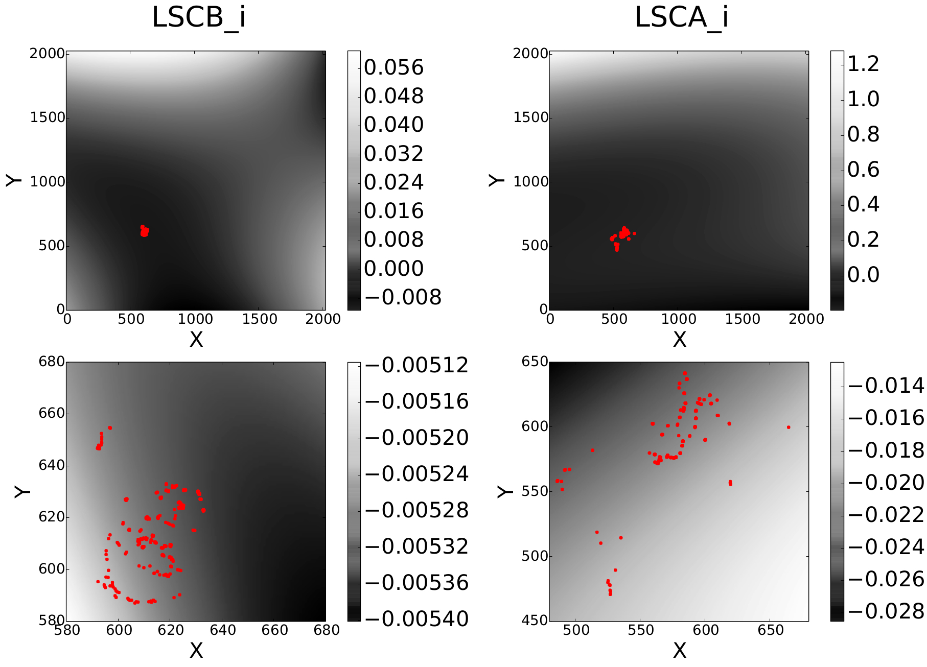
Figure 4.— Illumination correction for LSCB_i and LSCA_i data sets. The bottom figures are zoom close to the pointing area.

We chose also to study the LSCA_i data set because this telescope observed the target at the same time but does not show any planetary significance ($\Delta\chi^{2}\sim 20.7$). We conduct the same study and the results are summarized in Table  4 and Figure  4. The peak-to-peak amplitudes of the magnitude offsets are ten times bigger than for the LSCB_i dataset. It is surprising to see how two similar intruments can lead to such different data quality. A more careful check of the frames clearly shows a problem in the focus of the LSCA_i telescope. Because the Galactic Bulge fields are very crowded, this is a critical point for microlensing observations (e.g. increasing the blending). A plausible explanation of this difference between the twins is that during the time of observations, the telescopes were under commissioning, leading to non-optimal performance for LSCA_i.

IV.3. Auckland_R

We conducted the same study for the Auckland_R dataset because this telescope presents the clearest feature that mimics a planetary deviation, around $HJD\sim 6446.02$ as can be seen in Figure  3. Results can be seen in Table  4. Because the pointing for this dataset was extremely accurate (offset less than 2 pixels for the whole night of observation), the estimation of the illumination correction was not possible. There is not enough information in the matrix equations and they are degenerate. But this reflects the fact that the pointing did not induce systematic trends. However, a clear variation in the magnitude offset at each epoch is visible at the time of the deviation. Furthermore, we find that this offset is stronger for the brighter stars, as can be seen in Figure  5. There are strong similarities between the FSPL residuals and the magnitudes of the two brightest stars around the time of the anomaly $HJD\sim 6446.02$, especially when the FSPL residuals get brighter at $HJD\sim 6446.03$. Because the microlensing target is by far the brightest object in our field, we can expect that this systematics effect is probably even larger in our target. For this dataset, we slightly modified our strategy by computing the offset at each epoch only for the brightest stars ($mag<18$) and we rejected the microlensing target from the computation. Also, as can be seen in the bottom panel of Figure  5, the photometric scale factor shows variations during the night. This indicates the passage of clouds which can lead to systematics errors, as described previously. For example, the FSPL residuals in the interval $6446.01\leq HJD\leq 6446.02$ clearly share the pattern with the photometric scale factor.

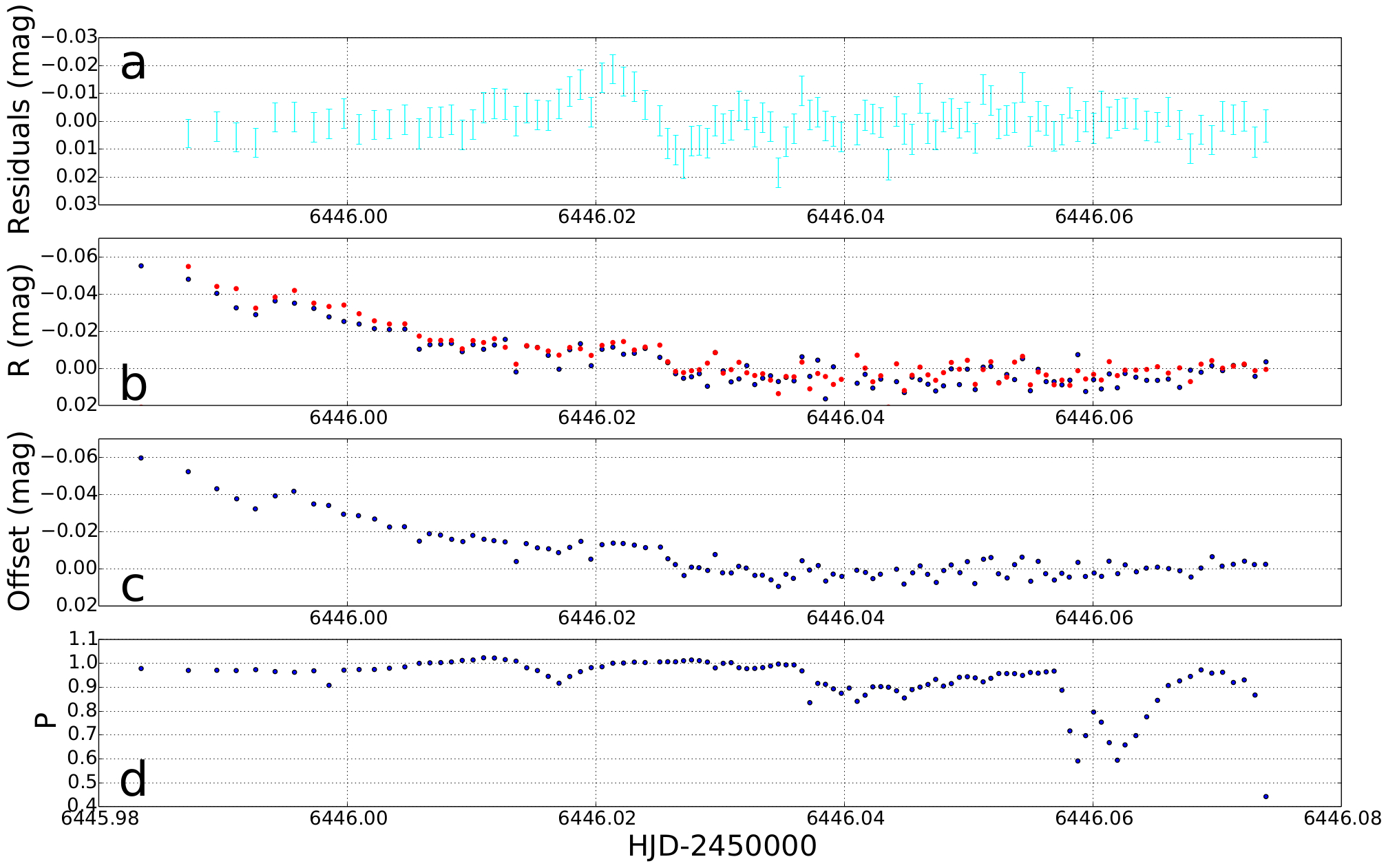
Figure 5.— a: Residuals of the FSPL model for the Auckland_R dataset. b: Light curves of the two other brightest stars in the field. c: Systematics magnitude offsets as a function of the epoch computed for this dataset, see text. d: Photometric scale factor (normalised to a single exposure).

IV.4. Correction of systematics

For the three studied datasets (LSCA_i, LSCB_i and Auckland_R), we corrected the systematics for the quantity that yielded the largest peak-to-peak amplitude in the magnitude offsets: namely the epoch. Moreover, this quantity is correlated with other quantities (airmass for example) and so the epoch correction should decrease the systematic trends measured for the other paramters listed in Table  4. We checked this and found that for the three datasets, the epoch correction leads to a significant improvement (order of a factor ten) for the systematics of the correlated quantities. This is a first order correction and we wanted to see the impact on the different models we analyzed. We repeated our modeling process with these new datasets using the previous models as starting points. The results are presented in Table 5. The new Auckland_R residuals can be seen in Figure  6. After correction, the amplitude of the ’anomaly’ is smaller but still exists. This is probably due to the fact that the amplitude of this feature in the light curves is brightness dependent , and the microlensing target is much brighter than all of the other stars, leading to an insufficient correcxtion fot the microlensing event.

Parameters	FSPL_c	FSPL_c+Annual parallax	FSPL_c+Terrestrial parallax	Wide planetary (FSBL_c)
$t_{o}$(HJD)	$6446.04818\pm 2~{}10^{-5}$	$6446.04681\pm 3~{}10^{-5}$	$6446.04680\pm 3~{}10^{-5}$	$6446.04665\pm 3~{}10^{-5}$
${\bf u_{o}}$($\theta_{E}$)	$-4.21~{}10^{-4}\pm 1~{}10^{-6}$	$-4.01~{}10^{-4}\pm 8~{}10^{-6}$	$-4.19~{}10^{-4}\pm 7~{}10^{-6}$	$-4.34~{}10^{-4}\pm 5~{}10^{-6}$
$t_{E}$(days)	$76.8\pm 0.1$	$80.6\pm 1.5$	$77.2\pm 1.3$	$74.9\pm 0.9$
$\rho$($\theta_{E}$)	$5.22~{}10^{-4}\pm 1~{}10^{-6}$	$4.97~{}10^{-4}\pm 4~{}10^{-5}$	$5.20~{}10^{-4}\pm 9~{}10^{-6}$	$5.40~{}10^{-4}\pm 7~{}10^{-6}$
$I_{s}$(mag)	$19.00\pm 0.01$	$19.05\pm 0.02$	$19.01\pm 0.02$	$18.97\pm 0.01$
$V_{s}$(mag)	$20.49\pm 0.01$	$20.55\pm 0.02$	$20.50\pm 0.02$	$20.46\pm 0.01$
$I_{b}$(mag)	$18.21\pm 0.01$	$18.19\pm 0.01$	$18.21\pm 0.01$	$18.23\pm 0.01$
$V_{b}$(mag)	$22.72\pm 0.10$	$22.35\pm 0.10$	$22.70\pm 0.11$	$22.98\pm 0.11$
$\Pi_{EN}$		$0.34\pm 0.12$	$0.05\pm 0.01$
$\Pi_{EE}$		$0.28\pm 0.04$	$-0.00\pm 0.01$
$s$($\theta_{E}$)				$1.50547\pm 0.04$
$q$				$2.304~{}10^{-5}\pm 1.9~{}10^{-6}$
$\alpha$(rad)				$-2.39\pm 0.02$
$\chi^{2}$	3647.999	3571.000	3625.150	3258.842

Table 5Model parameters after correction of systematics.

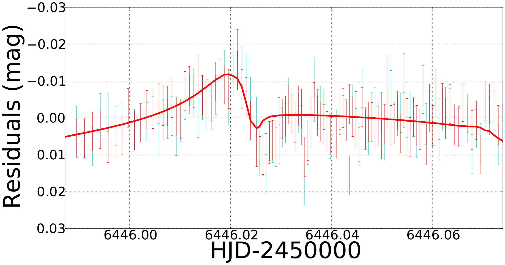
Figure 6.— FSPL residuals of the Auckland_R before (cyan) and after (red) correction for systematics using the magnitude offsets as a function of epoch. The best planetary model after correction (FSBL_c) is shown in red.

Telescope	RMS	Raw data			RMS	Corrected
	(mag)	$\chi^{2}_{FSPL}$	$\chi^{2}_{Pla}$	$\Delta\chi^{2}$	(mag)	$\chi^{2}_{FSPL}$	$\chi^{2}_{Pla}$	$\Delta\chi^{2}$
OGLE_I	0.029	770.308(459)	655.364(456)	114.944	0.029	765.677(459)	661.426(456)	104.251
OGLE_V	1.348	23.998(20)	24.005(17)	-0.007	1.348	23.998(20)	23.979(17)	0.019
Canopus_I	0.007	191.996(128)	132.410(125)	59.586	0.007	204.40(128)	137.769(125)	66.631
Auckland_R	0.006	142.839(103)	128.294(100)	14.545	0.006	112.917(103)	72.331(100)	40.586
LSCB_i	0.007	446.170(374)	317.883(371)	128.287	0.007	442.338(374)	311.049(371)	131.189
LSCA_i	0.015	399.723(381)	379.065(378)	20.658	0.013	173.683(381)	133.422(378)	40.261
CPTA_i	0.023	21.973(18)	21.926(15)	0.047	0.023	21.972(18)	21.925(15)	0.047
CTIO_I	0.006	159.174(108)	171.347(15)	-12.173	0.006	158.986(108)	167.376(105)	-8.48
CTIO_V	0.005	2.986(9)	5.385(6)	-2.399	0.005	3.036(9)	5.227(6)	-2.191
Danish_z	0.017	448.804(448)	470.960(445)	-22.156	0.017	450.589(448)	471.301(445)	-20.712
MOA_Red	0.785	727.979(450)	725.116(447)	2.863	0.783	727.760(450)	721.763(447)	5.997
Possum_N	0.012	355.767(240)	312.101(237)	43.666	0.012	354.002(240)	324.301(237)	29.701
Salerno_I	0.020	20.016(16)	18.911 (13)	1.105	0.020	19.990(16)	18.872(13)	1.118
Turitea_R	0.005	29.565(27)	29.341(24)	0.224	0.005	29.539(27)	28.965(24)	0.574
Weizmann_I	0.034	92.383(56)	92.667(53)	-0.284	0.034	92.389(56)	92.649(53)	-0.260
SAAO_I	0.014	67.100(54)	66.442(51)	0.658	0.014	67.085(54)	66 .487(51)	0.598
Total		3900.781	3551.217	349.564		3647.99	3258.842	389.157

Table 6$\chi^{2}$ and RMS of FSPL residuals for each data set before and after correction of systematics. The three corrected data sets are rendered in bold. Numbers in parentheses are the degrees of freedom for each model/data set.

As can be seen in Table  6, the correction of the systematics has a significant impact on the LSCA_i and Auckland_R data sets, which appear to suffer the most systematics. Note also that the planetary model is more significant after systematics correction, especially for these two telescopes. Even though the planetary model changes slightly before and after correction (the new $s$ and $q$ values are outside the error bars of the uncorrected data sets model), the caustic crossing is virtually unchanged (e.g the central caustic is similar). However, the clearest signature of the planetary anomaly is still in the Auckland_R dataset around $HJD\sim 6446.02$.

IV.5. Discussion

Due to strong finite source effects around a very small central caustic, the suspected planetary signature in OGLE-2013-BLG-0446 is very small. First of all, the low $\chi^{2}$ improvement ($\Delta\chi^{2}\sim 350$ and $\Delta\chi^{2}\sim 389$ before and after the sysematics correction respectively) of the planetary model is far from the minimum value generally adopted in microlensing for a safe detection Yee et al. (2013). Note also that even though the caustic crossing is similar, the two planetary models are not fully equivalent. As defined by Chung et al. (2005), the $R_{c}$ parameter is the ratio of the vertical length and the horizontal length of a central caustic. This caustic parameter before and after correction is significantly different ($\sim 30\%$). Secondly, the highest $\Delta\chi^{2}$ contributor (LSCB_i) presents photometric systematics at the same level as the planetary deviations (2 mmag versus 6 mmag). As can be seen in Figure  6, the systematics correction decreases the amplitude of the ’anomaly’ in the Auckland_R dataset and it is therefore better fit by the planetary model. However, the increase in the FSPL residuals after $HJD\sim 6446.02$ (from 1% to zero) is not explained by the planetary model, but similar behaviour is seen in other bright stars. This clearly indicates that bright stars suffer from systematic effects in this dataset which were not revealed by the different quantities we studied.

The planetary model is highly favoured by the Canopus_I dataset ($\Delta\chi^{2}\sim 60$). However, a closer look at Figure  3 reveals that the planetary deviations are at a very low level ($\leq 0.5\%$). It can not be excluded that the FSPL model correctly fits this data set and that this telescope also suffers from low level systematics errors. We however decided to not realize the same study of photometric systematic errors for the Canopus_I dataset because there is no obvious deviations in the FSPL residuals and also because enough doubt has already been place in the planetary model we found.

All these points reveal strong doubts about the reality of the planetary signature in OGLE-2013-BLG-0446. Even if we cannot firmly guarantee that the planet is not detected, we prefer to stay conservative and claim that we do not detect a planet in this event.

V. Conclusions

We presented the analysis of microlensing event OGLE-2013-BLG-0446. For this highly magnified event ($A\sim 3000$), several higher-order effects were investigated in the modeling process: annual and terrestrial parallax and planetary deviations. The study of photometric systematics for several data sets leads to various levels of confidence in the photometry. Moreover, a closer look at the data residuals and a precise study of photometric systematics reveals enough doubt to question any potential signals. Regarding the level of planetary signal ($\sim 1\%$) versus the various levels of systematics, we are not confident about the planetary signature in OGLE-2013-BLG-0446. Unfortunately, the clearest signature of the planetary signal was observed only in a single dataset which presents some unexplained behaviour for the brightest stars at the time of the anomaly. These doubts in addition to the relatively low improvement in $\chi^{2}$ ($\Delta\chi^{2}\leq 400$) encourage us to remain conservative and not to claim a planetary detection. This study stresses the importance of studying and quantifying the photometric systematic errors down to the level of 1 % or lower for the detecion of the smallest microlensing planets.

References

- Aigrain & Pont (2007) Aigrain, S. & Pont, F. 2007, MNRAS, 378, 741
- Albrow et al. (1999) Albrow, M. D., Beaulieu, J.-P., Caldwell, J. A. R., et al. 1999, ApJ, 522, 1011
- Albrow et al. (2009) Albrow, M. D., Horne, K., Bramich, D. M., et al. 2009, MNRAS, 397, 2099
- Bachelet et al. (2012a) Bachelet, E., Fouqué, P., Han, C., et al. 2012a, A&A, 547, A55
- Bachelet et al. (2012b) Bachelet, E., Shin, I.-G., Han, C., et al. 2012b, ApJ, 754, 73
- Beaulieu et al. (2006) Beaulieu, J.-P., Bennett, D. P., Fouqué, P., et al. 2006, Nature, 439, 437
- Bennett et al. (2014) Bennett, D. P., Batista, V., Bond, I. A., et al. 2014, ApJ, 785, 155
- Bennett & Rhie (1996) Bennett, D. P. & Rhie, S. H. 1996, ApJ, 472, 660
- Bessell & Brett (1988) Bessell, M. S. & Brett, J. M. 1988, PASP, 100, 1134
- Bond et al. (2001) Bond, I. A., Abe, F., Dodd, R. J., et al. 2001, MNRAS, 327, 868
- Bramich (2008) Bramich, D. M. 2008, MNRAS, 386, L77
- Bramich et al. (2015) Bramich, D. M., Bachelet, E., Alsubai, K. A., Mislis, D., & Parley, N. 2015, A&A, accepted
- Bramich & Freudling (2012) Bramich, D. M. & Freudling, W. 2012, MNRAS, 424, 1584
- Bramich et al. (2013) Bramich, D. M., Horne, K., Albrow, M. D., et al. 2013, MNRAS, 428, 2275
- Casagrande et al. (2010) Casagrande, L., Ramírez, I., Meléndez, J., Bessell, M., & Asplund, M. 2010, A&A, 512, A54
- Chung et al. (2005) Chung, S.-J., Han, C., Park, B.-G., et al. 2005, ApJ, 630, 535
- Claret (2000) Claret, A. 2000, A&A, 363, 1081
- Coccato et al. (2014) Coccato, L., Bramich, D. M., Freudling, W., & Moehler, S. 2014, MNRAS, 438, 1256
- Dominik et al. (2008) Dominik, M., Horne, K., Allan, A., et al. 2008, Astronomische Nachrichten, 329, 248
- Dong et al. (2009) Dong, S., Bond, I. A., Gould, A., et al. 2009, ApJ, 698, 1826
- Dong et al. (2007) Dong, S., Udalski, A., Gould, A., et al. 2007, ApJ, 664, 862
- Gould (1994) Gould, A. 1994, ApJ, 421, L71
- Gould (1997) Gould, A. 1997, ApJ, 480, 188
- Gould (2000) Gould, A. 2000, ApJ, 542, 785
- Gould (2004) Gould, A. 2004, ApJ, 606, 319
- Gould et al. (2009) Gould, A., Dong, S., Bennett, D. P., et al. 2009, arXiv0910.1832
- Gould & Loeb (1992) Gould, A. & Loeb, A. 1992, ApJ, 396, 104
- Gould et al. (2006) Gould, A., Udalski, A., An, D., et al. 2006, ApJ, 644, L37
- Gould & Yee (2013) Gould, A. & Yee, J. C. 2013, ApJ, 764, 107
- Griest & Safizadeh (1998) Griest, K. & Safizadeh, N. 1998, ApJ, 500, 37
- Hardy & Walker (1995) Hardy, S. J. & Walker, M. A. 1995, MNRAS, 276, L79
- Holz & Wald (1996) Holz, D. E. & Wald, R. M. 1996, ApJ, 471, 64
- Honeycutt (1992) Honeycutt, R. K. 1992, PASP, 104, 435
- Kains (2015) Kains, N. 2015, submitted
- Kervella & Fouqué (2008) Kervella, P. & Fouqué, P. 2008, A&A, 491, 855
- Kovács et al. (2005) Kovács, G., Bakos, G., & Noyes, R. W. 2005, MNRAS, 356, 557
- Mallén-Ornelas et al. (2003) Mallén-Ornelas, G., Seager, S., Yee, H. K. C., et al. 2003, ApJ, 582, 1123
- Milne (1921) Milne, E. A. 1921, MNRAS, 81, 361
- Miyake et al. (2012) Miyake, N., Udalski, A., Sumi, T., et al. 2012, ApJ, 752, 82
- Nataf et al. (2013) Nataf, D. M., Gould, A., Fouqué, P., et al. 2013, ApJ, 769, 88
- Nemiroff & Wickramasinghe (1994) Nemiroff, R. J. & Wickramasinghe, W. A. D. T. 1994, ApJ, 424, L21
- Paczyński (1986) Paczyński, B. 1986, ApJ, 304, 1
- Padmanabhan et al. (2008) Padmanabhan, N., Schlegel, D. J., Finkbeiner, D. P., et al. 2008, ApJ, 674, 1217
- Pepper & Gaudi (2005) Pepper, J. & Gaudi, B. S. 2005, ApJ, 631, 581
- Pont et al. (2006) Pont, F., Zucker, S., & Queloz, D. 2006, MNRAS, 373, 231
- Regnault et al. (2009) Regnault, N., Conley, A., Guy, J., et al. 2009, A&A, 506, 999
- Skottfelt et al. (2015) Skottfelt, J., Bramich, D. M., Hundertmark, M., et al. 2015, A&A, 574, A54
- Skowron et al. (2011) Skowron, J., Udalski, A., Gould, A., et al. 2011, ApJ, 738, 87
- Smith et al. (2012) Smith, J. C., Stumpe, M. C., Van Cleve, J. E., et al. 2012, PASP, 124, 1000
- Smith et al. (2003) Smith, M. C., Mao, S., & Paczyński, B. 2003, MNRAS, 339, 925
- Tamuz et al. (2005) Tamuz, O., Mazeh, T., & Zucker, S. 2005, MNRAS, 356, 1466
- Tsapras et al. (2009) Tsapras, Y., Street, R., Horne, K., et al. 2009, Astronomische Nachrichten, 330, 4
- Udalski (2003a) Udalski, A. 2003a, ApJ, 590, 284
- Udalski (2003b) Udalski, A. 2003b, Acta Astron., 53, 291
- Udalski & Szymański (2015) Udalski, A. & Szymański, M. 2015, Acta Astron., 65, 1
- Vermaak (2000) Vermaak, P. 2000, MNRAS, 319, 1011
- Witt & Mao (1994) Witt, H. J. & Mao, S. 1994, ApJ, 430, 505
- Yee et al. (2013) Yee, J. C., Hung, L.-W., Bond, I. A., et al. 2013, ApJ, 769, 77
- Yee et al. (2009) Yee, J. C., Udalski, A., Sumi, T., et al. 2009, ApJ, 703, 2082
- Yoo et al. (2004) Yoo, J., DePoy, D. L., Gal-Yam, A., et al. 2004, ApJ, 603, 139