Electrical phase diagram of bulk BiFeO₃

Abstract

We study the electrical behavior of multiferroic BiFeO₃ by means of first-principles calculations. We do so by constraining a specific component of the electric displacement field along a variety of structural paths, and by monitoring the evolution of the relevant physical properties of the crystal along the way. We find a complex interplay of ferroelectric, antiferroelectric and antiferrodistortive degrees of freedom that leads to an unusually rich electrical phase diagram, which strongly departs from the paradigmatic double-well model of simpler ferroelectric materials. In particular, we show that many of the structural phases that were recently reported in the literature, e.g. those characterized by a giant aspect ratio, can be accessed via application of an external electric field starting from the $R3c$ ground state. Our results also reveal ways in which non-polar distortions (e.g., the antiferrodistortive ones associated with rotations of the oxygen octahedra in the perovskite lattice) can be controlled by means of applied electric fields, as well as the basic features characterizing the switching between the ferroelectric and antiferroelectric phases of BiFeO₃. We discuss the multi-mode couplings behind this wealth of effects, while highlighting the implications of our work as regards both theoretical and experimental literature on BiFeO₃.

I Introduction

Our current understanding of ferroelectric materials is based on the concept of “soft mode”, a polar phonon that is unstable in the centrosymmetric reference phase and whose condensation leads to a spontaneous macroscopic polarization in the ferroelectric phase.Lichtensteiger et al. (2011) As a function of the soft mode amplitude, the energy landscape has typically a double-well shape, with a negative curvature at the origin due to the aforementioned instability, and a quartic (or higher order) positive term stabilizing the two ferroelectric minima. Recent research, however, has demonstrated that in many materials such a picture is way too simplistic: additional degrees of freedom often compete (or, sometimes, cooperate) with the polar modes in a nontrivial way, substantially complicating the energy landscape and consequently the phase diagram of the material. In most perovskites, these additional modes consist in strain degrees of freedom (deformation of the unit cell) and antiferrodistortive (AFD) tilts of the oxygen octahedra; magnetism is also very important, especially in the context of magnetoelectric multiferroic materials; finally there are some notable cases (and more are appearing weekly as this research topic has been gaining considerable momentum recently) where antiferroelectric (AFE) modes play an important role as well. All these lattice distortions, taken individually, are nonpolar in nature, but their coupling (either mutual or to the polar modes) often leads to unusual and potentially useful physical properties, of interest to both information and energy technologies. Understanding such couplings is crucial to devising new materials with enhanced properties, and to gaining new fundamental insight into the rich physics that these compounds display.

BiFeO₃ is an especially attractive material in this context, and it has been intensely studied in the past few years as it remains one of the very few known room-temperature multiferroics (i.e. compounds where ferroelectricity and magnetism coexist in the same phase). In its ground-state phase, BiFeO₃ adopts a distorted perovskite structure with $R3c$ symmetry, where the spontaneous ferroelectric polarization coexists with antiphase AFD tilts, and both are oriented along the [111] pseudocubic direction. Recent studies, both experimentalZeches et al. (2009); Guennou et al. (2011) and theoretical,Diéguez et al. (2011); Hatt et al. (2010); Wojdeł and Íñiguez (2010); Yang et al. (2012) have revealed that BiFeO₃ is a true polymorphic material: in addition to the ground-state $R3c$ structure, it can adopt a rich variety of low-energy metastable phases. Some of these phases, characterized by peculiar physical properties (e.g. a monoclinic structure with a giant $c/a$ ratio, where $c$ and $a$ are the out-of-plane and in-plane lattice parameters), can be stabilized via application of an epitaxial strain in a thin-film sample. Interestingly, in many of these metastable states, distortion patterns (e.g. AFE, or in-phase AFD) that are not present in the ground state appear, pointing to a complex behavior that largely escapes the traditional models of ferroelectrics. Thus BiFeO₃ provides us with a unique playground to explore the interplay of competing order parameters, how they interact with external perturbations (e.g. strain, electric fields, etc.) and how these interactions may lead to enhanced functional properties.

From the point of view of first-principles theory, a significant number of studies have focused on using strain as a means to exploring the available configuration space,Hatt et al. (2010); Wojdeł and Íñiguez (2010); Yang et al. (2012) in order to simulate epitaxial thin-film growth conditions. Such studies have been very successful at revealing key physical features, e.g. the isosymmetric transition from the ground-state rhombohedral structure to the “supertetragonal” phase under strong in-plane compression.Hatt et al. (2010) However, relying on just strain as an external parameter provides a necessarily limited perspective of the energy landscape, especially in the present case where many order parameters coexist. Another option that has also been quite successful is the so-called “effective Hamiltonian” approach,Zhong et al. (1994); Kornev et al. (2007) which consists in analyzing the phonon spectrum of the high-symmetry reference phase and the energetics of the dominant structural instabilities, and using such information to build an approximate low-energy model of the system under consideration. This allows to study the behavior of the material in a larger variety of conditions, for example at finite temperature or under an applied electric field.Lisenkov et al. (2009) Such an approach is most accurate when the amplitude of the distortion is relatively small, and the number of higher-order terms that one needs to incorporate in the Hamiltonian is limited. In other cases, e.g. perovskites based on the lone-pair-active cations Pb or Bi, anharmonicities are much stronger, and writing a reliable functional with a small number of terms (and degrees of freedom) becomes more problematic.Diéguez et al. (2011)

Recently, methodologies have appeared that allow one to go beyond many of the limitations described above, by directly controlling the electrical variables (polarization and electric field) in a simulation of a crystalline insulator.Souza et al. (2002); Stengel and Spaldin (2007) In particular, the possibility of performing a calculation at a fixed value of the electric displacement field (the so-called “constrained-$D$” technique)Stengel et al. (2009) enables the study of the direct interaction between polar and other (AFD, AFE, elastic, magnetic) degrees of freedom. This is of great help for identifying the microscopic couplings that govern the stability of a given phase, understanding the nature of the switching paths (and potential barriers) between two local minima, and ultimately enrichening our perspective on the mechanisms that are most relevant for the functional properties of interest (piezoelectricity, magnetoelectricity).

Here we perform a detailed study of bulk BiFeO₃ by means of the constrained-$D$ technique. In particular, by considering four different paths in electric displacement space, we develop a comprehensive map where most of the relevant low-energy phases can be readily located, clarifying their mutual relationship. Furthermore, the evolution of all relevant degrees of freedom is studied along each path, providing unique insight into their coupling to the polar vector. We show that the paradigmatic double-well potential of simple ferroelectrics becomes, in the case of BiFeO₃, either a three- or a four-well potential curve depending on the chosen path, with several phase transitions (either first- or second-order) occurring along the way. Of particular note, we identify an important region of the phase diagram where the physics is dominated by strong antiferroelectric displacements of the Bi atoms, whose switching behavior under an applied field is fundamentally interesting even beyond the specifics of BiFeO₃. (In fact, we could not find earlier works where the field-induced switching of an antiferroelectric phase is studied from first principles, except for a couple of recent investigations based on approximate potentials.Xu et al. (2015a, b)) Interestingly, we could also identify some ranges of $D$ values where BiFeO₃ displays complex tilts (i.e. an in-phase and anti-phase AFD mode coexisting along the same axis), which appears to be a rare occurrence in the physics of simple perovskites.

II Methods

Our calculations are performed within the local density approximation to density functional theory, with an on-site Hubbard $U$ ($U=3.3$ eV) applied to the $3d$ orbitals of Fe. The core-valence interactions are dealt with in the framework of the projector-augmented wave method,Blöchl (1994) with a plane-wave cutoff of 50 Ry. We use a 20-atom monoclinic BiFeO₃ cell, which we construct as follows. Let ${\bf a}_{1,2,3}$ be the real-space translation vectors of a hypothetical 5-atom perovskite cell; then the corresponding 20-atom cell is defined by $\bar{\bf a}_{3}=2{\bf a}_{3}$, $\bar{\bf a}_{1}={\bf a}_{1}-{\bf a}_{2}$, and $\bar{\bf a}_{2}={\bf a}_{1}+{\bf a}_{2}$. (Note that, even if our calculations are always performed with the 20-atom cell, in some cases we find it convenient for presentation purposes to convert our data into the 5-atom cell representation by inverting the above formulas; such instances are clearly marked in the text.) The larger $\sqrt{2}\times\sqrt{2}\times 2$ cell allows us to describe, in addition to the ferroelectric polarization (${\bf P}$), the magnetic order (we assume G-type antiferromagnetism throughout) and the relevant structural distortions. These are in-phase antiferrodistortive tilts of the oxygen octahedral network along $z$ (AFD${}_{z}^{+}$), anti-phase AFD modes along all Cartesian axes (AFD${}_{x,y,z}^{-}$) and possible antiferroelectric modes. The Brillouin zone of the 20-atom cell is sampled with a special $k$-point set that is equivalent to a $4\times 4\times 4$ Monkhorst-Pack sampling of the primitive (5-atom) perovskite unit.

The fundamental variable in the context of this work is the electric displacement vector, ${\bf D}$,

$${\bf D}=\epsilon_{0}\bm{\mathcal{E}}+{\bf P}.$$

In practice, in the BiFeO₃ results presented here, the contribution of the electric field to ${\bf D}$ is always negligible compared to that of ${\bf P}$; therefore, when looking at the graphs, we can assume that we are essentially fixing the corresponding polarization component to a given target value.

We perform our calculations by constraining only one component of the reduced (see Section II.1) electric displacement field $\hat{\bf D}$ at the time, thus mimicking a parallel-plate capacitor with a fixed free charge at the surface. The choice of the component of $\hat{\bf D}$ corresponds to fixing a certain crystallographic orientation for the surface. In this work we shall work with either the $\hat{D}_{001}$ (“out of plane”, also indicated as $\hat{D}_{z}$) or the $\hat{D}_{110}$ (“in plane”, also indicated as $\hat{D}_{xy}$) component, corresponding to the $[001]$ and $[110]$ pseudocubic directions, respectively. The calculation is repeated several times while varying the relevant component of $\hat{\bf D}$ (and hence while describing a path in electric displacement space); at each point, the energy, internal electric field, and all structural distortions of interest are monitored and analyzed. Note that we often find several coexisting phases at certain values of $\hat{D}$, and sometimes the structure undergoes an abrupt change within a small interval of $\hat{D}$; whenever such changes are discontinuous, we shall identify them as first-order phase transitions, second-order otherwise.

II.1 Note on the parameters used in the analysis

Since the system undergoes substantial relaxations of the cell shape and volume as a function of ${\bf D}$, it is extremely convenient Stengel et al. (2009) to represent all quantities (electrical and structural) in reduced coordinates. First, in addition to the real-space translation vectors, it is helpful to introduce the “dual” reciprocal-space vectors, $\bar{\bf b}_{1,2,3}$, in such a way that

$$\bar{\bf a}_{i}\cdot\bar{\bf b}_{j}=\delta_{ij}.$$

Then, in close analogy with the definition of the reduced atomic coordinates, we introduce the reduced electric displacement field and polarization (both with the dimension of a charge) as

$$\hat{D}_{i}=\Omega\bar{\bf b}_{i}\cdot{\bf D},\qquad\hat{P}_{i}=\Omega\bar{\bf b}_{i}\cdot{\bf P}.$$

The reduced electric field is, instead, written as

$$\hat{E}_{i}=\bar{\bf a}_{i}\cdot\bm{\mathcal{E}}$$

and has the dimension of a voltage. In the remainder of this work we shall indicate the relevant components of $\hat{\bf D}$ by $[ijk]$ or $xyz$ subscripts, which better clarify their orientation with respect to the pseudocubic axes. One should keep in mind, however, that the $\bar{\bf b}_{i}$ and $\bar{\bf a}_{i}$ triads that appear in the above definition are rotated, as they refer to the 20-atom cell that we used in the calculations. Whenever needed, one can easily convert between the two references (such a conversion will be performed systematically, e.g. when presenting the results for the “rigid-ion” polarization, which we shall introduce shortly). It is important to stress, in this context, that the “reduced” electrical variables that we just introduced are extensive physical quantities, i.e. they depend both on the choice of unit cell axes and on cell size. The simulated cell can be simply thought as a parallel-plate capacitor: $\hat{E}$ is the applied voltage, and $\hat{D}$ is the total polarization and displacement charge that has flowed through the cell facet. Both evidently grow with the size of the system, if the applied electric field is kept constant.

In addition to the energy, internal field, electric displacement and cell parameters, we further analyze our structures by extracting the amplitude of four inequivalent AFD distortions (see figure captions) and the reduced “rigid-ion” polarization. The latter is a vector sum of the reduced atomic positions in the 20-atom cell, each weighted by the nominal ionic charge of each specie (+3 for Bi and Fe, $-$2 for O). From this value we remove a fixed number of “quanta of polarization” in order to ensure that the result vanishes in centrosymmetric phases. The primary reason for considering this quantity and not the Berry phase polarization is that the latter is only available along the field direction in our in-house first-principles code. This is not a major issue: despite of the quantitative discrepancy, the qualitative behavior (especially in relation to symmetries) of the rigid-ion ${\bf P}$ is analogous to that of the full Berry-phase ${\bf P}$. Nevertheless, it should be kept in mind that genuine electronic effects (e.g. anomalies in the Born dynamical charge tensor, or response of the electron cloud to the macroscopic electric field) are absent from the rigid-ion ${\bf P}$.

III Results

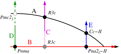
Figure 1: Schematic phase diagram of BiFeO₃. The horizontal and vertical axes correspond to $P_{001}$ and $P_{110}/\sqrt{2}$, respectively. The five different paths (A, B, C, D, E) in electric displacement space that were considered in this work are represented by lines/curves with arrows. The most relevant phases are indicated by circles (filled and empty circles are used, respectively, for local minima and saddle points). The dashed portion of line D indicates that the corresponding path follows a potential ridge, rather than a valley (symmetry was imposed by hand to constrain the system along the $P_{001}=0$ line). The thinner portion of line C indicates that the polarization acquires an out-of-plane component there; this path, therefore does not cross path B – the phase marked $R3c$ at $P_{110}=0$ bears a different color as a reminder.

Phase	$\Delta E$	$P_{xy}$	$P_{z}$	AFD pattern
$R3c$	0	76.8	54.2	$(a^{-}a^{-}a^{-})$
$Cc$-II	98	42.1	140.1	$(a^{-}a^{-}c^{-})$
$Pnma$	26	0	0	$(a^{-}a^{-}c^{+})$
$Pna2_{1}$-II	101	0	141.5	$(a^{-}a^{-}c^{+})$
$Pmc2_{1}$-II	106	116.1	0	$(a^{0}a^{0}c^{+})$
$Pmc2_{1}$ (*)	69	83.4	0	$(a^{-}a^{-}c^{+})$
$Ima2$ (*)	72	94.0	0	$(a^{-}a^{-}c^{0})$

Table 1: Relative energy, spontaneous polarization and AFD distortion pattern of the main phases of BiFeO₃ discussed in this work. The energy ($\Delta E$), in meV per formula unit, is referred to the $R3c$ ground state. The polarization vector is reported in units of $\mu$C/cm² ($xy$ refers to the in-plane component, $z$ to the out-of-plane one). The notation for the AFD pattern follows that of Glazer.Glazer (1975) Star symbols in the first column indicate phase that are not local minima but saddle points.

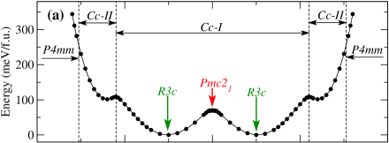
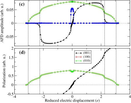
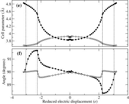
Figure 2: Evolution of the system along path A, obtained by starting from the $R3c$ ground state of BiFeO₃ and varying $\hat{D}_{001}$. (a): Energy (the zero is set to the the $R3c$ ground state); (b): internal electric field; (c): anti-phase AFD${}_{z}^{-}$ (filled black triangles), AFD${}_{x,y}^{-}$ (empty red circles and green diamonds, respectively), and in-phase AFD${}_{z}^{+}$ (filled blue squares) amplitudes, (d): rigid-ion polarization vector (the same convention as in the AFD^- case is used to label the individual $x$, $y$ and $z$ components); (e): $|{\bf a}_{3}|$ (filled circles) and $|{\bf a}_{1,2}|$ (empty circles); (f): angle formed by ${\bf a}_{1}$ and ${\bf a}_{2}$ (empty circles), and by ${\bf a}_{3}$ and ${\bf a}_{1,2}$ (filled circles). Data in (e-f) are referred to the 5-atom cell; values of the reduced electric displacement field, $\hat{D}_{001}$, are referred to the 20-atom cell. Vertical dashed lines indicate second-order phase transitions.

In order to explore the phase diagram of BiFeO₃ as a function of the electrical degrees of freedom, we investigate the evolution of the equilibrium crystal structure along five selected paths in electric displacement space, as schematically illustrated in Fig. 1. These were obtained by using one of the lowest-energy (meta)stable phases of BiFeO₃ as a starting point, and by subsequently constraining either $\hat{D}_{001}$ or $\hat{D}_{110}$ to the physically relevant range of values. ($\hat{D}_{001}$ or $\hat{D}_{110}$ indicate, respectively, the projection of the reduced electric displacement vector, $\hat{\bf D}$, along either the out-of-plane [001] or the in-plane [110] pseudocubic axis.) The majority of the resulting phases (the main ones are explicitly indicated in Fig. 1) present a $(\bar{1}10)$ mirror-symmetry plane; in such cases, $\hat{D}_{\bar{1}10}$ vanishes, and the resulting structures can be conveniently mapped on a two-dimensional diagram spanned by $\hat{D}_{001}$ and $\hat{D}_{110}$. An exception to this rule occurs along path C, where the system acquires a nonzero value of $\hat{P}_{\bar{1}10}$, and hence breaks the aforementioned mirror symmetry.

Before discussing the specifics of each path, it is useful to briefly summarize (both for future reference and for comparison with earlier works) the main phases of BFO that we have encountered in our study. In Table 1 we report the energy (relative to the $R3c$ ground state), spontaneous polarization and AFD distortion pattern characterizing each phase. The overall picture appears to be well in line with existing literature data;Diéguez et al. (2011) there are some minor differences at the quantitative level, which are most likely due to the choice of the pseudopotential and/or other computational parameters.

III.1 Path A

We start from the fully relaxed $R3c$ ground state of BiFeO₃ (at $\hat{D}\sim 1.0$ in Fig. 2) and vary $\hat{D}_{001}$, i.e. apply an electric field along the out-of-plane pseudocubic direction (corresponding to the reciprocal-space vector $\bar{\bf b}_{3}$). At the energy minimum, the internal electric field [panel (b)] vanishes, all AFD^- [panel (c)] and ${\bf P}$ [panel (d)] components are equal, as well as the cell parameters [(e)] and angles [(f)]; this is fully consistent with the rhombohedral symmetry of the relaxed crystal. In a vicinity of the global minimum the symmetry reduces to monoclinic $Cc$ – we shall refer to this region as $Cc$-I, in loose analogy to earlier works. (In the recent literature, $Cc$-I has often been used to indicate the phase of BiFeO₃ that results from the application of an epitaxial strain; the present case of an electric field perturbation at relaxed cell parameters yields a similar structure of the same symmetry, hence our naming choice.) The symmetry breaking produced by the field is obvious in all relevant degrees of freefom of the system: The $\hat{P}_{001}$ component of the polarization grows at the expense of the in-plane one [Fig. 2(d)], and a similar behavior characterizes the anti-phase AFD^- vector [Fig. 2(c)]; also, the $c/a$ ratio increases, as well as the monoclinic angle [panels (e) and (f), respectively].

At a sufficiently large field, BiFeO₃ undergoes an isosymmetric transition to a structure with a much larger polarization and axial ratio. The transition is accompanied by a drastic suppression of the AFD${}^{-}_{001}$ mode and a significant change in the monoclinic angle of the cell. Such a structure has been the topic of several studies in the recent past, and will be indicated as $Cc$-II henceforth. Note that this structure is a local minimum, and that the transition is continuous, i.e. of second-order character. A further increase in the electric displacement field produces a progressive increase of the aspect ratio and a reduction of the AFD${}^{-}_{110}$ amplitude and of the monoclinic angle. At $\hat{D}_{001}\sim 3.1$, both AFD${}^{-}_{110}$ and $\hat{P}_{110}$ go to zero, and the crystal adopts the higher $P4mm$ (tetragonal) symmetry. Note that $P4mm$ is not a metastable state, nor even a saddle point in our simulations. In fact, such a structure can be sustained only by an unrealistically large electric field, at the limit of what one can afford even in a computer simulation. We consider it unlikely that such extreme conditions may be accessible in the laboratory. (Yet, it is possible to obtain such a $P4mm$ phase by growing thin films on strongly compressive substrates.Christen et al. (2011))

When moving towards smaller $\hat{D}_{001}$ values (which corresponds to applying an $\mathcal{E}$-field antiparallel to $\hat{P}_{001}$), the out-of-plane components of both the polarization and the AFD vector are progressively suppressed, as expected, while the in-plane components tend to a constant. In a vicinity of the saddle point at $\hat{D}_{001}=0$, however, something quite unexpected happens: The in-phase AFD${}_{z}^{+}$ mode softens, eventually inducing a second-order phase transition to a configuration where both AFD${}_{z}^{-}$ and AFD${}_{z}^{+}$ coexist. To explain such an outcome, recall that AFD${}_{z}^{+}$ is an active instability of the cubic reference phase; yet, in the ground state $R3c$ phase such a mode is stabilized by its strong biquadratic repulsion with AFD${}_{z}^{-}$. The strong suppression of AFD${}_{z}^{-}$ at $\hat{D}_{001}\sim 0$ brings AFD${}_{z}^{+}$ back into play, explaining the second-order transition. At this point, AFD${}_{z}^{-}$ should become stable as the two distortions are mutually exclusive; hovever, the existence of a small residual out-of-plane component of ${\bf P}$ “drives” the AFD^- vector to acquire an out-of-plane component as well, even if such a distortion is no longer an active lattice instability. (The coupling responsible for such an effect will be discussed in Section IV.1.) When $\hat{D}_{001}$ is forced to be exactly zero, the system recovers a $(001)$ mirror plane, and the symmetry becomes $Pmc2_{1}$. Note that a stable phase of this same symmetry was recently predicted to occur in BiFeO₃ thin films at very large tensile strain. The present $Pmc2_{1}$ phase differs from the previously reported one in that it is unstable with respect to an out-of-plane polar distortion, and has an aspect ratio that is close to $1:1$. Thus, the present $Pmc2_{1}$ phase can be regarded, as far as $\hat{P}_{001}$ is concerned, as a “centrosymmetric” reference structure for the $R3c$ ground state. ($Pmc2_{1}$, of course, is not centrosymmetric overall, as it is characterized by a large $\hat{P}_{110}$.)

III.2 Path B

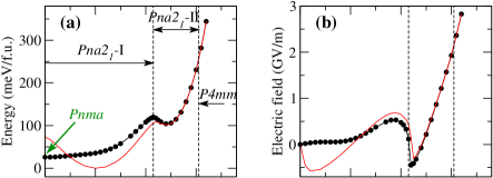
Figure 3: Evolution of the system along path B, obtained by starting from the $Pnma$ metastable state of BiFeO₃ (at $\hat{\bf D}=0$) and varying $\hat{D}_{001}$. (a): Energy (filled circles); (b): internal electric field (filled circles); (c): anti-phase AFD${}_{z}^{-}$ (filled black triangles), AFD${}_{x,y}^{-}$ (empty red circles and green diamonds, respectively), and in-phase AFD${}_{z}^{+}$ (filled blue squares) amplitudes, (d): antiferroelectric (AFE) mode amplitude; (e): $|\bar{\bf a}_{3}|$ (filled circles); (f): $|{\bf a}_{1}|$ (empty circles) and $|{\bf a}_{2}|$ (squares). Data in (e-f) are referred to the 20-atom cell (we use a red color to distinguish them from the 5-atom cell data that are presented in other plots). Values of the reduced electric displacement field, $\hat{D}_{001}$, are referred to the 20-atom cell. Red curves without symbols in (a-b) refer to path A [same as in Fig. 2(a-b)], and are shown here for comparison. Vertical dashed lines indicate second-order phase transitions.

Excluding the $R3c$ structural ground state, the lowest-energy (meta)stable configuration of BiFeO₃ is the $Pnma$ phase. It is natural, therefore, to perform an analogous computational experiment as above (i.e. by controlling $\hat{D}_{001}$), but this time using $Pnma$ as starting point. Note that the polarization identically vanishes in the centrosymmetric $Pnma$ phase, so this “path B” in electric displacement space passes through the origin (see Fig. 1). As we shall see, the system preserves two mirror planes for all values of $\hat{D}_{001}$: The ${\bf P}$ vector stays parallel to the $z$ axis, and the lattice remains orthorhombic.

In Fig. 3(a-b) we show the internal energy and electric field that we obtained along this path; for comparison, we also report the corresponding physical quantities that we have calculated along path A (see Section III.1). The electrical properties of the system look very different in the central region of the phase diagram, i.e. for small to intermediate values of $\hat{D}_{001}$. At $\hat{D}_{001}=0$, the $Pnma$ state largely wins over the unstable $Pmc2_{1}$ state discussed earlier. While increasing $\hat{D}_{001}$, the energy difference between the two configurations becomes smaller, until the corresponding curves sharply cross at $\hat{D}_{001}\sim 0.5$. For higher $\hat{D}_{001}$ values the path-A structures become favorable, until the curves merge at very large fields ($\hat{D}_{001}\sim 3.1$) into the same supertetragonal ($P4mm$) structure. Several things are interesting to note here, as we shall illustrate in the following.

First, the energy as a function of $\hat{D}$ displays a remarkably flat plateau around $\hat{D}_{001}\sim 1.0$, pointing to an unusual dielectric softness of the lattice in that region of parameter space. Closer inspection of the corresponding evolution of the electric field [Fig. 3(b)] shows a slight dip around the same value of $\hat{D}_{001}$ – this indicates that the system is on the verge of having a metastable minimum there, of $Pna2_{1}$ symmetry and an out-of-plane ${\bf P}$ of about 0.5 C/m². Interestingly, earlier calculations indicate that a $Pna2_{1}$ metastable state with these characteristics indeed exists.Diéguez et al. (2011) However, only gradient-corrected functionals seem to lead to a local minimum – such a structure was not found whithin LDA, consistent with our present results. This $Pna2_{1}$ state can be thought as the original $Pnma$ structure, with a AFD${}_{z}^{+}$, AFD${}_{xy}^{-}$ tilt pattern, plus a symmetry-lowering out-of-plane polarization [see Fig.3(c)], which in our case is “barely not spontaneous” (i.e. it is induced by the electric field).

Second, note the presence of a strong antiferroelectric distortion [Fig. 3(d)] at essentially all values of $\hat{D}_{001}$, except for the very largest ones ($\hat{D}_{001}>3.0$). Such an AFE mode is, in many perovskites, a direct consequence of the $Pnma$-like tilt pattern, which induces an antiparallel displacement of the A-site cations (Bi in this case) in different (001) atomic planes.Bellaiche and Íñiguez (2013) The lone-pair activity of the Bi cations, however, leads to a distortion amplitude that is unusually large (i.e. much larger that one would expect if the AFE mode were only a secondary effect of the tilts). We shall go back to the specific role played by the AFE distortion in the following Sections, where we study the effects of an in-plane oriented electric field.

Finally, note the region $1.5<\hat{D}_{001}<3.0$. Here the energetics and the electrical properties of the system [Fig. 3(a-b)] qualitatively follow the same evolution regardless of whether we are considering path A or path B. Such an observation has two logical implications: (i) even if the structures along paths A and B are quite different (in-plane ${\bf P}$ and AFD${}_{z}^{-}$ in the former case, in-plane AFE and AFD${}_{z}^{+}$ in the latter), their response to an out-of-plane field (and therefore the couplings between such distortions and $\hat{P}_{001}$) must be comparable; (ii) the very similar energies of the two metastable minima encountered along these paths, respectively $Cc$-II and $Pna2_{1}$-II (the energy difference at the secondary minimum, $\hat{D}_{001}\sim 2.5$, approximately amounts to 3 meV per formula unit), suggest that it might be possible to switch between these two phases upon application of an in-plane field; such a study will be taken on in Section III.5.

III.3 Path C

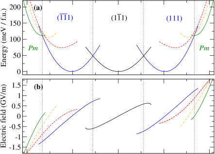
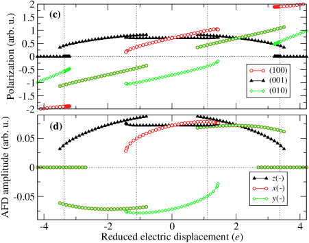
Figure 4: Evolution of the system along path C, obtained by starting from the $R3c$ ground state, and varying $\hat{D}_{110}$ via an in-plane electric field. (a): Energy (a different color or line style is used to highlight different segments in configuration space); (b): internal electric field; (c): anti-phase AFD${}_{z}^{-}$ (filled black triangles), AFD${}_{x,y}^{-}$ (empty red circles and green diamonds, respectively); (d): components of the rigid-ion polarization. Vertical dotted lines indicate second-order phase transitions; horizontal dotted lines in (c) and (d) mark the zero of the graph. The zero of the energy is set to the $R3c$ ground state, as usual.

In order to gain further insight on the electrical behavior of BiFeO₃, it is particularly interesting to apply, starting from the $R3c$ ground state, an electric field along the in-plane [110] direction, rather than [001] as we did for path A. We expect this study to shed some light on how ferroelectric switching proceeds in this material, e.g. whether the polarization vector prefers to continuously rotate (as it is customarily assumed), or rather jump at once from one orientation to the other. It will be also interesting to clarify how the other order parameters (i.e. those that are not directly acted upon by the electric field) evolve during switching. Of course, a realistic simulation of switching would require a much more sophisticated theory, including temperature and disorder effects. Here we focus on the (necessarily limited) information that can be extracted from a hypothetical zero-temperature experiment, where the sample is forced to remain single-domain throughout the electrical cycle.

The internal energy and electric field as a function of the reduced electric displacement, $\hat{D}_{110}$, are shown in Fig. 4(a-b); the evolution of the internal degrees of freedom, respectively polarization and AFD modes, is plotted in Figs. 4(c) and 4(d). Note, in Fig. 4(a), the presence of three degenerate global minima, all corresponding to the ground-state $R3c$ structure, but with the polarization vector oriented in different directions: At $\hat{D}\sim\pm 2$, ${\bf P}$ is parallel to [111], while at $\hat{D}=0$ it is oriented along [$1\bar{1}1$]. When the displacement field is varied around each of these minima, the material behaves like a standard dielectric, with the internal electric field growing linearly with $\hat{D}$ [black and blue curves in Fig. 4(b)]. The evolution of the internal degrees of freedom [Fig. 4(c-d)] is, however, rather different depending on whether the electric field acts perpendicular to the spontaneous ${\bf P}$ (as in the central region of the diagram) or at $\sim 35$ degrees to it (as in the regions surrounding $\hat{D}\sim 2$). At $\hat{D}=0$, we have a replica of the $R3c$ ground state, where both ${\bf P}$ and the AFD vector are oriented along the $[1\bar{1}1]$ direction; all components of the corresponding (pseudo)vector quantities are equal in absolute value. By applying an electric field along [110], $P_{001}$ remains roughly constant, while both $P_{100}$ and $P_{010}$ undergo a linear increase. AFD${}^{-}_{z}$ remains also constant, while the in-plane components progressively rotate away from the $[1\bar{1}0]$ direction, moving towards $[100]$; this behavior is in line with the known tendency of the AFD vector to align with ${\bf P}$. At large enough values of the displacement field (around $\hat{D}\sim 1.5$), the structure loses stability and an abrupt transition occurs to the neighboring phase; note that the energy curves cross each other somewhat earlier (at $\hat{D}\sim 1$), confirming the first-order nature of the corresponding field-induced transition. In the course of this transition, two main things happen: (i) the $P_{1\bar{1}0}$ component [red curve in Fig. 4(c)] drops to zero (i.e. $P_{100}$ and $P_{010}$ become equal); (ii) the $y$ component of the AFD^- pseudovector [diamond symbols in panel (d)] switches sign, adopting the same value as AFD${}^{-}_{x}$. Both facts unambiguously indicate that the crystal has switched to a different configuration. In fact, this structure reduces to the [111]-oriented $R3c$ phase at $\hat{D}\sim 2.0$. These results indicate that the polarization does not follow the paradigmatic picture that is usually assumed for ferroelectric materials, i.e. that of a smooth rotation between one state and the closest symmetry equivalent. The polar degrees of freedom seem to abruptly jump, instead, between different configurations. We ascribe this behavior to the peculiar chemistry of the Bi cation, whose lone pair is prone to forming rather stiff bonds with the neighboring atoms. It is reasonable to speculate that the Bi ions, as they are pulled away from their equilibrium position by a strong enough field, prefer to break free and directly switch site, rather than gradually moving through the transition state. (Our conclusions are in line with a recent first-principles investigation in which the lowest-energy transition paths for ferroelectric switcihng in BiFeO₃ were computed.Heron et al. (2014))

When forcing the in-plane polarization to larger values (i.e. at either extreme, left or right, of the graphs in Fig. 4), a new structure appears, of $Pm$ symmetry. As one can see from Fig. 4(c-d), here all the AFD distortions disappear; conversely, there is a large in-plane polarization, with a larger component along $[100]$ and a smaller one along $[010]$. While increasing $\hat{D}_{110}$ (and hence $\hat{E}_{110}$), this phase again behaves like a linear dielectric material, as one can appreciate from Fig. 4(b).

The transition to the $Pm$ phase is another example of the peculiar behavior of BiFeO$3$, which largely deviates from what one would expect from common wisdom. In fact, one would naively think that, by applying a [110]-oriented field, one would end up increasing $P_{110}$ at the expense of $P_{001}$ and, in parallel, increasing AFD${}^{-}_{xy}$ at the expense of AFD${}^{-}_{z}$, until both order parameters eventually align with [110]. This would yield a hypothetical phase of $Ima2$ symmetry. In order to check whether this scenario might apply to our case, we constrained by hand the symmetry of the system to $Ima2$ and investigated how the resulting structure responds to a varying electrical displacement field. The results for the energy and internal electric field are shown as dashed lines in Fig. 4(a-b). Looking at the energy graphs, the high-$\hat{D}$ part of the blue curve seems indeed to join smoothly the dashed red curve, as one would expect from a second-order transition to $Ima2$. However, before this happens, the system loses stability and spontaneously falls into the $Pm$ state, which thereafter remains stable at arbitrarily large values of the electric field. As a result, the hypothetical transition to $Ima2$ never occurs, contrary to the conclusions of Ref. Lisenkov et al., 2009.

To further corroborate our finding of $Pm$ being the ground state at large $\hat{D}_{110}$ values, we have examined one more alternative structure, of $Pmc2_{1}$ symmetry. (We indicate this metastable phase as $Pmc2_{1}$-II, to distinguish it from the unstable $Pmc2_{1}$-I phase that will be detailed in Sec. III.4.) Our motivation for considering this trial structure comes from Ref. Yang et al., 2012, where an analogous phase characterized by a large [110]-oriented polarization and an AFD${}^{+}_{z}$ distortion was found to become favorable at large tensile strain. As it can be appreciated from the corresponding curves in Fig. 4(a) (orange dot-dashed), the energy is lower than that of the $Ima2$ phase over the whole relevant range of $\hat{D}_{110}$, confirming that $Pmc2_{1}$-II is indeed a valid low-energy candidate. However, the $Pm$ structure is clearly favored over $Pmc2_{1}$-II, in agreement with the result of Ref. Lisenkov et al., 2009 that a $Pm$ structure becomes stable in the high-field regime.

III.4 Path D

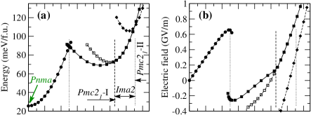
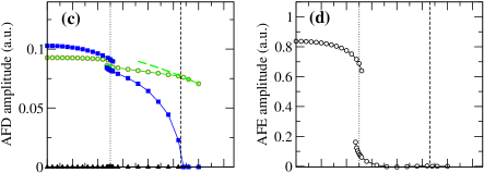
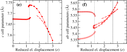
Figure 5: Evolution of the system along path D, obtained by starting from the $Pnma$ metastable state of BiFeO₃ (at $\hat{\bf D}=0$) and varying $\hat{D}_{110}$ via an in-plane electric field. (a): Energy. $Pmc2_{1}$ symmetry is imposed by hand in the data points shown as filled symbols; empty symbols refer to an analogous calculation where we impose the higher $Ima2$ symmetry; different symbols (circles, squares, diamonds) are used to highlight separate segments in configuration space. (b): Internal electric field [same symbol convention as in panel (a)]. (c): Anti-phase AFD${}_{z}^{-}$ (filled black triangles), AFD${}_{x,y}^{-}$ (empty red circles and green diamonds, respectively), and in-phase AFD${}_{z}^{+}$ (filled blue squares) amplitudes, (d): Antiferroelectric (AFE) mode amplitude. (e): $|\bar{\bf a}_{3}|$ (filled circles); the dashed line refers to the calculations with imposed $Ima2$ symmetry. (f): $|{\bf a}_{1}|$ (empty circles) and $|{\bf a}_{2}|$ (squares). Data in (e-f) are referred to the 20-atom cell. Values of the reduced electric displacement field, $\hat{D}_{110}$, are referred to the 20-atom cell. Red curves without symbols in (a-b) refer to path A [same as in Fig. 2(a-b)], and are shown here for comparison. Vertical dashed lines indicate second-order phase transitions.

The $Pnma$ phase described in Section III.2 and the $Pmc2_{1}$ phase described in Section III.1 have several things in common. In fact, all distortions are qualitatively similar, except that the former has an AFE pattern in plane, while the latter is characterized by an in-plane ${\bf P}$. Based on this observation, it seems reasonable to suppose that one could switch the AFE pattern of $Pnma$ into the FE pattern of $Pmc2_{1}$ by applying an in-plane field. What remains to be seen is whether this will happen at physically realistic values of the electric field, $\mathcal{E}$, and if yes, how the AFD modes behave along this path. (Note that this path does not always follow the bottom of a valley in the two-dimensional electrical displacement diagram; the instability of the $Pmc2_{1}$ state indicates that, at least in some segments of this path, the system may follow a ridge. To prevent the system from falling into the adjacent basins, we impose $Pmc2_{1}$ symmetry by hand throughout the path.)

In Fig. 5 we show the results of the aforementioned computational experiment. At small values of the in-plane field, the $Pnma$ phase behaves like a linear dielectric, with the energy increasing quadratically as a function of $\hat{D}_{110}$. [Note that the electric field, shown in Fig. 5(b), is an almost perfectly linear function of $\hat{D}_{110}$.] In the same interval, the amplitude of AFD${}_{z}^{+}$ undergoes a small reduction, especially at larger fields, but remains large throughout; the other AFD modes show little change.

At $\hat{D}_{110}$ values slightly larger than 1.0, an abrupt transition occurs, where the electric field suddenly switches sign. This transition is associated with the reorientation of the electrical dipoles of the cell, whose ordering goes from antiferro to ferro [the evolution of the AFE amplitude is shown in Fig. 5(d)]. Remarkably, the AFD${}_{z}^{+}$ mode survives even after the transition, although at a slightly reduced amplitude. The antiferroelectric Bi displacement pattern, therefore, is not necessarily a prerequisite to having a AFD${}_{z}^{+}$ distortion, although these two modes clearly cooperate. Indeed, even after the transition to a ferroelectric ordering, a small AFE component survives, most likely as a secondary effect of the AFD${}_{z}^{+}$ mode. (This is complementary to the example of Section III.5, where a small AFD${}_{z}^{+}$ amplitude develops as a secondary effect of the large AFE distortion.)

By increasing the in-plane polarization the AFD${}_{z}^{+}$ mode becomes progressively weaker, until it disappears completely at $\hat{D}_{110}>2.7$. Here, the system undergoes a second-order transition to a phase of (higher) $Ima2$ symmetry. (As we mentioned in the previous section, this phase is, again, unstable – it could occur in this specific example solely because of the imposed symmetry constraints.) If we perform a backward sweep starting from the $\hat{D}_{110}>2.7$ region, and progressively decrease the field while imposing the $Ima2$ symmetry by hand, we obtain the energy and field values that are represented as empty symbols in Fig. 5(a-b). The difference between these new points and the original ones (which were obtained within the lower $Pmc2_{1}$ symmetry) illustrates how much energy is gained (and how the relevant properties of the system are altered) by the condensation of the AFD${}_{z}^{+}$ tilts. [The evolution of the AFD${}_{x,y}^{-}$ amplitude and of the cell parameters in the $Ima2$ phase is shown as dashed curves in Figs. 5(c) and 5(e-f).]

At even larger values of $\hat{D}$, the system eventually adopts the $Pmc2_{1}$-II structure that we described earlier. (We omitted the structural information about this phase in the figures, to avoid overcharging them with redundant data.) This phase is stable at large fields; its energy and internal field are indicated by a dashed line with diamond symbols in Fig. 5(a-b).

III.5 Path E

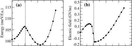
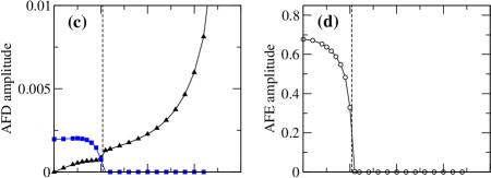
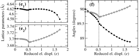
Figure 6: Evolution of the system along path E, obtained by starting from the $Pna2_{1}$-II state, and varying $\hat{D}_{110}$ via an in-plane electric field. (a): Energy. (b): Internal electric field. (c): Anti-phase AFD${}_{z}^{-}$ (filled black triangles), and in-phase AFD${}_{z}^{+}$ (filled blue squares) amplitudes (AFD${}_{x,y}^{-}$ mode amplitudes remain roughly constant throughout, and are not shown). (d): Antiferroelectric (AFE) mode amplitude. (e): $|{\bf a}_{3}|$ (filled circles) and $|{\bf a}_{1,2}|$ (empty circles). (f): angle formed by ${\bf a}_{1}$ and ${\bf a}_{2}$ (empty circles), and by ${\bf a}_{3}$ and ${\bf a}_{1,2}$ (filled circles). Data in (e-f) are referred to the 5-atom cell, as in Fig. 2. Values of the reduced electric displacement field, $\hat{D}_{110}$, are referred to the 20-atom cell. The vertical dashed line indicates a second-order phase transition.

In Fig. 3(a) we have, at $\hat{D}_{001}\sim$2.5, two almost overlapping minima. The lower one, of $Cc$ symmetry, is reached by progressively increasing $\hat{D}_{001}$ from the ground-state $R3c$ phase (red curve). It is characterized by a high aspect ratio with a noticeable tilt of the $c$ axis [see Fig. 2(f)], both in-plane and out-of-plane components of the polarization [the latter is much larger, see Fig. 2(d)], and anti-phase AFD distortions along all three directions (AFD${}_{x,y}^{-}$ are both significant, while AFD${}_{z}^{-}$ is small). The other (3 meV higher in energy) local minimum, of $Pna2_{1}$ symmetry, is reached when starting from $Pnma$ (black curve). It is similar to the $Cc$-type minimum that we have just discussed, except for a few important details: the $c$ axis is not tilted; the in-plane components of ${\bf P}$ vanish identically, and are replaced by a significant in-plane AFE distortion; the small (anti-phase) AFD${}_{z}^{-}$ is replaced by an equally small (in-phase) AFD${}_{z}^{+}$. If it weren’t for such small AFD_z components and for the AFE pattern, one could think of the latter phase as the “centrosymmetric” reference structure for the former when the polarization is switched in plane. If this were true, it would be reasonable to expect the $Pna2_{1}$ phase to be a saddle point for switching, and therefore be unstable. This is, however, not the case: both phases are local minima. A possible hypothesis to explain this outcome is that the either the small AFD${}_{z}^{+}$ distortion or the AFE mode play a key role in stabilizing $Pna2_{1}$.

To shed some light on this point, and investigate whether (and how) it may be possible to electrically switch the system between the $Pna2_{1}$-II and $Cc$-II states, we have performed a study similar to that of Section III.4, i.e. applying an in-plane field along [110], but this time starting from $Pna2_{1}$-II. As shown in Fig. 6(a), the energy first grows quadratically as a function of $\hat{D}$ [note the initially linear evolution of $\mathcal{E}$ in panel (b)], and a small AFD${}_{z}^{-}$ component appears (as a consequence of the tilting of the ${\bf P}$ vector away from the vertical axis); interestingly, here (in close analogy to the situation discussed in the context of path A) both AFD${}_{z}^{-}$ and AFD${}_{z}^{+}$ coexist for a certain range of $\hat{D}$ values. At larger values of $\hat{D}_{110}$, the dielectric response of the system progressively softens, and the AFE modes undergo an increasingly drastic suppression. Eventually, a second-order transition occurs that is driven by the disappearence of the AFE modes. At the same time, the AFD${}_{z}^{+}$ modes also disappear (recall that they are a secondary effect of the AFE distortion in this region of the electrical phase diagram). At even larger fields, the AFD${}_{z}^{-}$ modes progressively grow in magnitude, and the system overall recovers a linear dielectric behavior.

Thus, we can conclude that the strong AFE distortions (the amplitude of the AFE mode in $Pna2_{1}$ is comparable to that in the $Pnma$ phase: Bi atoms move by about 0.19 Å and 0.29 Å from their “ideal” position in the $Pna2_{1}$ and $Pnma$ structures, respectively), rather than the small AFD${}_{z}^{+}$ modes drive the transition between $Pna2_{1}$-II and $Cc$-II. One can think in the following terms. Imagine a hypothetical “reference” structure, obtained from the $Pna2_{1}$ by removing both the AFE and AFD${}_{z}^{+}$ modes. Such a structure has an unstable polar branch, reflecting the marked tendency of the Bi atoms to off-center in-plane. If we condense the zone-boundary mode, we obtain the AFE $Pna2_{1}$ state. The AFE mode, in turn, couples with the AFD${}_{z}^{+}$ mode: even if the latter is stable in this region of the BiFeO₃ phase diagram, it “feels” the large amplitude of the former, and is therefore brought slightly off its equilibrium position. (In other words, we can regard the AFD${}_{z}^{+}$ distortion as a consequence of the AFE mode, the latter acting on the former as a “geometric field”. The couplings responsible for such an effect are described in Section IV.1.) Conversely, if we go back to the reference structure and condense the zone-center polar mode, there is no driving force whatsoever for an AFD${}_{z}^{+}$ distortion to appear. Instead, the uniform $\hat{P}_{xy}$ couples cooperatively with AFD${}_{z}^{-}$. As before, the latter mode is stable and would not occur by itself – only as a secondary effect of having $\hat{P}_{xy}$. (The cooperative coupling is obvious from the progressive increase of the AFD${}_{z}^{-}$ amplitude for increasingly large values of the in-plane electric displacement field, $\hat{D}_{xy}$.)

IV Discussion

IV.1 Couplings

The main couplings that are of relevance for this work are between polarization and AFD modes, polarization and strain, and antiferroelectricity and AFD modes. The ${\bf P}$-AFD coupling is well known in BiFeO₃, as it tends to align the anti-phase AFD pseudovector with the polar ${\bf P}$ vector.Kornev et al. (2006, 2007) In particular, consider the following term, which is quartic in the mode amplitudes,

$$E^{{\rm AFD}-{\bf P}}=D\hat{P}_{xy}\hat{P}_{z}\omega^{-}_{xy}\omega^{-}_{z}.$$ (1)

(Here $\omega_{i}$ indicates the amplitute of the $AFD^{-}_{i}$ mode, following the notation of Refs. Kornev et al., 2006 and Kornev et al., 2007. In our simulations along path A we calculate, for $\hat{D}_{001}\sim 0$, large values of both $\hat{P}_{xy}$ and $\omega^{-}_{xy}$ (both tend to a finite constant at $\hat{D}_{001}=0$). In such a regime, Eq. (1) states that $\omega^{-}_{z}$ must grow linearly with $\hat{P}_{z}$ at small values of the latter, which is indeed what we observe. Along path D, on the other hand, we start from a situation (at $\hat{D}_{110}=0$) where $\hat{P}_{z}$ and $\omega^{-}_{xy}$ are both large, while the other two degrees of freedom vanish. Application of an in-plane electric field induces a small $\hat{P}_{xy}$, which in turn linearly induces a comparatively small $\omega^{-}_{z}$ due to the coupling in Eq. (1). (This coupling is precisely responsible for the coexistence of out-of-phase and in-phase octahedral rotations along the $z$ axis.)

Another important coupling of interest in the context of this work is the well-known trilinear term in the AFE, $\omega^{-}_{xy}$ and $\omega^{+}_{z}$,

$$E^{{\rm AFE}-\bm{\omega}}=CQ_{\rm AFE}\omega^{-}_{xy}\omega^{+}_{z}.$$ (2)

In presence of large $\omega^{-}_{xy}$, this term yields a cooperative coupling between $Q_{\rm AFE}$ and $\omega^{+}_{z}$. This means that the energy will be significantly lowered when the two instabilities condense together (and thus possibly explain the surprisingly low energy of the $Pnma$ phaseDiéguez et al. (2011) – it is only few meVs higher than that of the $R3c$ ground state). Also, in those regions of the phase diagram where only one of the latter two modes is an active instability of the system, the stable mode will feel a “geometric field” that forces it slightly off-center. We have seen examples of such a behavior along both path D and path E: in the former, a small $Q_{\rm AFE}$ amplitude persists even in a region of the phase diagram where the $Q_{\rm AFE}$ mode is no longer “soft” (i.e. for $\hat{D}_{110}>1.25$), see Fig. 5(d); in the latter, a small $\omega^{+}_{z}$ is present at $|\hat{D}_{110}|<0.5$, see Fig. 6(c) [the fact that $\omega^{+}_{z}$ is a secondary effect of $Q_{\rm AFE}$ there can be inferred from the evolution of these two order parameters along path B].

IV.2 Behavior as a function of applied electric field

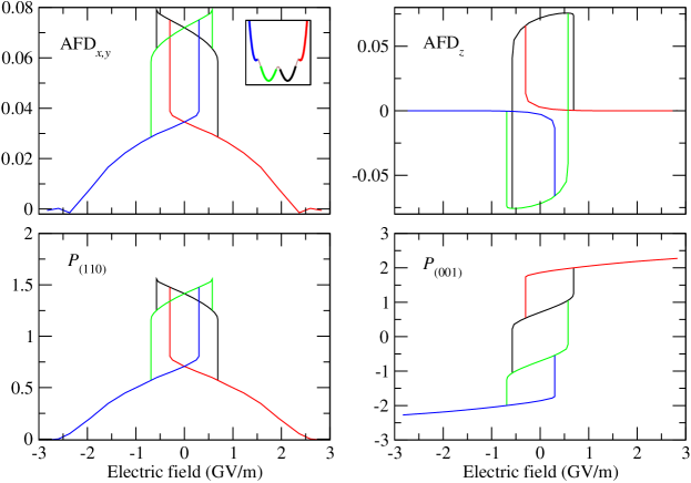
Figure 7: Switching via a [001]-oriented electric field. The four main panels represent the evolution of the relevant order parameters as a function of the applied field. The inset represents the potential energy curve [same as in Fig. 2(a)], where the various segments have been highlighted according to the color code used in the main panels (unstable regions are marked in brown). Polarization and AFD amplitudes are in arbitrary units (consistent with the fixed-$\hat{D}$ plots presented earlier).

We can use our results to inspect the behavior of BiFeO₃ as a function of applied electric field, rather than the reduced electric displacement. This way we are able to simulate a hypothetical ferroelectric switching experiment, performed at zero temperature and by constraining the sample to remain in a monodomain configuration throughout. This also allows us to compare our results with those of previous first-principles-derived approaches, e.g. those of Ref. Lisenkov et al., 2009.

We shall discuss two different switching paths, obtained respectively by applying an electric field along the pseudocubic [001] or [110] directions. Interestingly, such information can also be used to access important functional properties of BiFeO₃, and their evolution under an external field of arbitrary magnitude. For example, a recent experimental work has reported a significant nonlinearity in the electromechanical response of BiFeO₃, with an increase of the piezoelectric coefficient at high fields;Chen et al. (2012) we shall address this topic in the last part of this Section.

IV.2.1 Switching along [001]

To represent the evolution of the system as a function of the electric field, we start from the data discussed in Section III.1, referring to path A in electric displacement space. First, we identify the segments where the system is in a (meta)stable state, i.e. the parts of the curves where the electric field increases for increasing $\hat{D}_{001}$. (The remainder of the data points are characterized by a negative capacitance, and as such they correspond to unstable regions of the electrical phase diagram.) Then, we replace the abscissas with the calculated value of the internal electric field, and finally we connect the different segments with vertical jumps wherever appropriate. Note that such jumps always occur when a given phase reaches its limit of (meta)stability, i.e. when a small increase in the electric field magnitude produces a large variation in the structural parameters, indicating a transition to a different phase. These transitions are hysteretic, i.e. the system usually can be switched back to the original phase, but at a different critical field value.

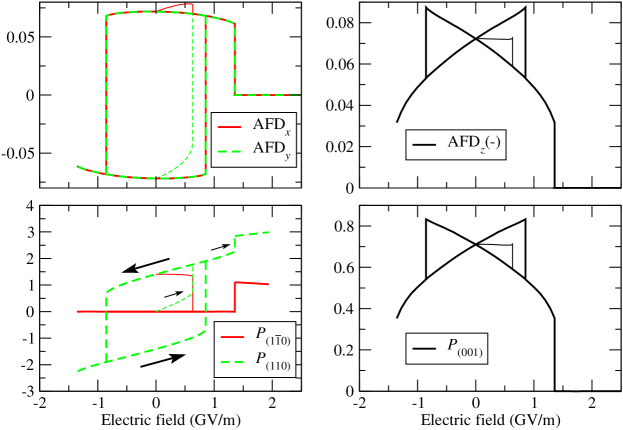
Figure 8: Switching via a [110]-oriented electric field. As the paths described by the system are uncomplicated to follow, we have reverted to the usual color code of the manuscript. Thinner lines refer to the evolution of the system when the initial state is the $\hat{D}_{110}=0$ configuration of Fig. III.3. Large arrows indicate the direction along which the system evolves within the main hysteresis loop. Small arrows indicate the evolution of the systems along secondary paths that lead into (or, alternatively, out from) the main loop. Polarization and AFD amplitudes are in arbitrary units (consistent with the fixed-$\hat{D}$ plots presented earlier).

The resulting plots are shown in Fig. 7. In the four different panels we show, respectively, the AFD amplitude (top) and the three components of the “rigid-ion” polarization; the inset illustrates, as a guide, the color code that we used to represent the different segments. Note the multivalued character of the graphs, which is typical of multistable ferroeoectric materials. At difference with common ferroelectrics, however, BiFeO₃ displays four different states at zero field, corresponding respectively to the two stable and two metastable minima in the energy curve (inset). As expected, the graphs referring to in-plane components are symmetric with respect to an electric field inversion, while the out-of-plane ones are antisymmetric. At low to moderate fields, the AFD pseudovector behaves identically to the polarization vector. Conversely, at high fields AFD${}^{-}_{z}$ drops abruptly to zero while the corresponding component of the polarization keeps increasing ($Cc$-II phase). At very high fields, also the in-plane AFD components go to zero, and the system transitions to the $P4mm$ phase. From our data, we can extract the four critical fields that will bring the system through the following path: $Cc$-II$(-)$, $Cc$-I$(-)$, $Cc$-I$(+)$, $Cc$-II$(+)$, $P4mm$$(+)$. These are, respectively, 0.30 GV/m, 0.57 GV/m, 0.69 GV/m, and $\sim$2.3 GV/m. Note that the sequence of transitions is different from that of Ref. Lisenkov et al., 2009: the $Cc$-II phase was presumably not known when Lisenkov et al. constructed their effective Hamiltonian, and the authors were therefore unaware of the two corresponding metastable minima. Even regarding the transition [$Cc$-I$(-)$ $\rightarrow$ $Cc$-I$(+)$] that was studied in Ref. Lisenkov et al., 2009, our results show important differences at the quantitative level. Most importantly, the critical field of Ref. Lisenkov et al., 2009 appears to be largely overestimated with respect to ours ($\sim 1.5$ GV/m vs. our value of 0.57 GV/m). This discrepancy probably originates from the approximations that are typically used to build a simplified effective model. These consist in discarding all the electronic and most of the lattice degrees of freedom, preserving only few active variables in the problem. As noted by others,Diéguez et al. (2011) we suspect that BiFeO₃ might be a particularly difficult material in this context, because of the strong nonlinearities induced by the lone-pair activity of Bi, which lead to a remarkably rich and complex energy landscape. Here many degrees of freedom interact in a highly nontrivial way, making a simplified description particularly tricky.

It is interesting to note that the transition to a phase with large aspect ratio ($Cc$-II) occurs, according to our results, at a relatively small value of the electric field, 0.69 GV/m. This may be within experimental reach (values up to 0.28 GV/m were probed in Ref. Chen et al., 2012), and thus open new opportunities for the study of the supertetragonal phase of BiFeO₃.

IV.2.2 Switching along [110]

Here we perform the same post-processing procedure described earlier, only applying it to path C [which refers to an electric field applied along the [110] direction] instead than path A. The results are shown in Fig. 8. When applying a [110]-oriented field to the $R3c$ structural ground state, one can obtain different results depending on the orientation of the spontaneous polarization in the initial state. If we start with ${\bf P}\sim[1\bar{1}1]$, the field is initially perpendicular to ${\bf P}$, and will tend to rotate the polarization vector towards the $[111]$ direction; the evolution of the relevant structural degrees of freedom along this path is illustrated by thin lines in Fig. 8. As we observed above, however, the rotation of ${\bf P}$ does not proceed smoothly, but instead happens abruptly once the limit of stability of the $[1\bar{1}1]$-oriented phase is attained. In particular, at first $P_{001}$, $P_{1\bar{1}0}$ and AFD${}^{-}_{z}$ remain constant while both $P_{110}$ and AFD${}^{-}_{x,y}$ increase linearly. For larger fields some nonlinearities show up, until eventually, at a critical field of 0.63 GV/m, the system transitions to the [111]-oriented structure. [Note that, once such a transition has occurred, the system will not go back to the $[1\bar{1}0]$-oriented state, hence the absence of a corresponding hystheresis loop in the plots.] For larger fields, the polarization component that is collinear with the field, $P_{110}$, keeps increasing at the expense of $P_{001}$ and AFD${}^{-}_{z}$; in the same interval AFD${}^{-}_{x,y}$ remain roughly constant (actually, our results show a slight decrease). At a second critical field of 1.36 GV/m, the system switches to the $Pm$ state described in Section III.3, where the AFD distortions disappear completely and a large polarization develops along an off-axis in-plane direction.

If after the first transition, from the $[1\bar{1}1]$- to the [111]-oriented phase, instead of further increasing the electric field we decrease it again to zero, we end up in the [111]-oriented $R3c$ ground state. From here, by applying a negative field, we obtain the opposite result compared to above, i.e. $P_{110}$ decreases while both $P_{001}$ and AFD${}^{-}_{z}$ simultaneously increase. At a sufficiently large negative field of $-$0.85 GV/m, the system switches directly to a $[\bar{1}\bar{1}1]$-oriented state; as we said above, this happens without visiting ever again the $[1\bar{1}1]$ region of the phase diagram. Here, AFD${}^{-}_{x,y}$ and $P_{110}$ both switch sign, while $P_{001}$ and AFD${}^{-}_{z}$ remain positive, in spite of undergoing a significant reduction.

This latter observation is in qualitative disagreement with the simulations of Ref. Lisenkov et al., 2009, where all the components of ${\bf P}$ were found to switch simultaneously when a sufficiently large [110]-oriented field is applied to a $[\bar{1}\bar{1}1]$-type $R3c$ starting point. The reasons behind such a discrepancy are presently unknown. We can only speculate that the dynamics of the transition might play a role (in our calculations we evolve the system quasistatically along the switching path, while some thermal activation is considered in Ref. Lisenkov et al., 2009). Or, alternatively, subtle differences in the potential landscape (possibly associated with the effective Hamiltonian generation procedure) might be the real culprit. Further calculations and cross-checks will be necessary to clarify this point. Apart from this, the critical fields that we obtain here appear to be, again, much smaller than those calculated by Lisenkov et al. For example, reversal of the in-plane polarization occurs in our calculations at a field of 0.85 GV/m, compared to the value of 1.62 GV/m reported in Ref. Lisenkov et al., 2009. At higher fields, Lisenkov et al. report a transition to a $Ima2$ state, which in our calculations never occurs, at a field of 4.26 GV/m, and a second transition to $Pm$ at 5.5 GV/m. We find, instead, that the system transitions directly to $Pm$, without passing through the $Ima2$ state (the $Ima2$ phase appears to be unstable at any value of the electrical displacement field in our calculations), and at a substantially smaller field of 1.36 GV/m. Such a large difference in the critical fields suggests that the potential landscapes of our BiFeO₃ model and that of Ref. Lisenkov et al., 2009 significantly differ, which would justify the aforementioned discrepancy in our respective switching paths.

IV.2.3 Piezoelectric coefficient at high field

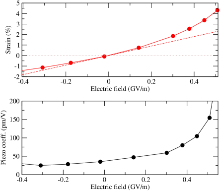
Figure 9: Piezoelectric coefficient as a function of the applied electric field.

Chen et al.Chen et al. (2012) have recently studied the piezoelectricity of a BiFeO₃ thin film, and found that at high electric fields the response deviates significantly from the low-field values. In particular, the out-of-plane strain component displays a strong nonlinearity, reaching values of up to 2% at the highest fields (0.28 GV/m); consequently, the piezoelectric constant increases from 55 pm/V up to 86 pm/V. This outcome was ascribed to the lattice softening that occurs in the proximity of a phase transition; the electric field would drive the system close to the $Cc$-II state, and thus induce the observed nonlinearities.

Verifying such a scenario is relatively straightforward with the data that we already have in our hands. It suffices, along path A, to express the $c$ parameter of the cell as a function of the applied potential, $V$; then, the piezoelectric coefficient is readily given by differentiating the former with respect to the latter. (Strictly speaking, our data should be compared with some caution to those of Ref. Chen et al., 2012: in the latter the in-plane lattice parameters are clamped to the substrate, and do not show any variation with the applied field; in our computational experiment, all structural parameters of the cell are left free to relax.)

The results for the equilibrium out-of-plane strain and piezoelectric constant are shown, as a function of the applied field in Fig. 9. At high values of the field, the system undergoes a drastic increase of the $c$ parameter, reaching a strain of 4% at $E\sim$0.5 GV/m; at 0.3 GV/m the strain is about 2%, in nice agreement with the experimental data of Ref. Chen et al., 2012. Such a strongly nonlinear behavior (the hypothetical linear regime is represented by a thin dashed line, for comparison) is clearly a consequence of lattice softening in proximity of the $Cc$-II phase, confirming the arguments of Chen et al. – as we said, the transition itself occurs in our calculations at fields (0.69 GV/m) that are only slightly larger than those shown in Fig. 9. The piezoelectric coefficient at zero field is significantly smaller in our calculations than in Ref. Chen et al., 2012: 37 pm/V versus 55 pm/V. (This may be a consequence of our use of the LDA approximation, which tends to harden the phonon frequencies and hence the lattice response to a field.) Nevertheless, the field-induced increase appears to be in excellent agreement: from 37 pm/V to 60 pm/V in our calculations, versus 55 pm/V to 86 pm/V in the experiment, i.e., about 60% in both cases.

IV.3 Stability under an applied field

Figure 10: Phase stability as a function of the applied electric field. (a): energy versus a [001]-oriented electric displacement under an applied external voltage $V_{\rm ext}$ = 0.33 V. (b): energy versus a [110]-oriented electric displacement under an applied external voltage $V_{\rm ext}$ = 0.41 V.

In the examples above, the transition between different phases was determined by the stability range of the starting point, without regards for the relative energetics of the final configuration. Because of the assumption of an ideal monodomain crystal, the resulting critical fields are largely overestimated, e.g. with respect to the experimental coercive fields. Defects and/or inhomogeneities in a real material typically facilitate switching by providing nucleation centers and alternative transition paths (e.g. via domain wall motion). This needs to be kept in mind when comparing our results with the available experimental data.

From our data there, however, one can extract other pieces of information that are, in principle, much less sensitive to the above issue. In particular, one may be interested in the stability range of a given phase, rather than in the actual transition path that leads from one phase to another. More concretely, one can ask the following question: “What voltage do I need to apply to the sample in order for a given phase to be the structural ground state?” In the context of our fixed-$D$ calculations, answering this question is particularly easy – it only involves operating a simple modification to the total energy curves that takes into account the applied external voltage. This implies, in practice, adding a linear function to the internal energy,

$$U^{\prime}(\hat{D})=U(\hat{D})+V_{\rm ext}\hat{D},$$ (3)

where $V_{\rm ext}$ is the external bias applied to the relevant facet of the simulation cell. The critical voltage corresponds then to the value of $V_{\rm ext}$ for which two configurations, belonging to two separate segments of the electrical equation of state, become degenerate in energy. (The situation is in all respects analogous to the study of phase stability under applied mechanical stress; the electric displacement field can be thought as the “volume” coordinate, whereas the applied voltage is the counterpart of the hydrostatic pressure.)

In Fig. 10 we show the results of such an analysis, which we performed in the two cases described in the previous Section of [001]-oriented and [110]-oriented voltage drops, respectively. An external voltage of 0.33 V/cell is sufficient to make the supertetragonal $Cc$-II phase degenerate with the lowest-energy point in the $Cc$-I region. This is, therefore, the minimum voltage that is necessary for the high-field $Cc$-II phase to become accessible; it corresponds to an electric field of about 400 MV/m and is, therefore, very close to the experimentally accessible range. The corresponding analysis of the [110]-oriented case leads to a stability limit of the $Pm$ phase of 0.41 V/cell, corresponding to a comparatively larger electric field of 700 MV/m. Note that this critical value is, in any case, significantly smaller than 1.36 GV/m, which we found in the previous Section when studying the actual transition.

V Conclusions

We have studied the electrical phase diagram of bulk BiFeO₃ by describing four different paths in electric displacement space. Four important aspects of the physics of BiFeO₃ emerge from the results presented here: (i) the presence of nontrivial couplings between the polar and other structural degrees of freedom; (ii) the possibility of controlling antiferrodistortive modes of BiFeO₃ via application of an electric field; (iii) the relevance of antiferroelectricity in some regions of the electrical phase diagram, where it leads to a characteristic triple-well potential as a function of $\hat{D}_{110}$ [one can regard (ii) and (iii) as consequences of (i)]; (iv) the five-well potential of BiFeO₃ as a function of $\hat{D}_{001}$, which results from the presence of a metastable $Pnma$ phase at small values of $\hat{D}_{001}$, and of a high-aspect ratio $Cc$ phase at large values of $\hat{D}_{001}$.

The above results provide original physical insight into the complex energy landscape of BiFeO₃, which can be taken as a model system to study the interplay between different structural modes and, in particular, the competition between ferroelectric and antiferroelectric phases. Our results also constitute a stringent benchmark for future development of approximate (e.g. effective Hamiltonian) models.