A review of the neutrino emission processes in the late stages of the stellar evolutions

Abstract

In this paper the neutrino emission processes being supposed to be the main sources of energy loss in the stellar core in the later stages of stellar evolution are reviewed. All the calculations are carried out in the framework of electro-weak theory based on the Standard Model. It is considered that the neutrino has a little mass, which is very much consistent with the phenomenological evidences and presupposes a minimal extension of the Standard Model. All three neutrinos (i.e., electron neutrino, muon neutrino and tau neutrino) are taken into account in the calculations. It is evident that the strong magnetic field, present in the degenerate stellar objects such as neutron stars, has remarkable influence on some neutrino emission processes. The intensity of such magnetic field is very close to the critical value ($H_{c}=4.414\times 10^{13}$ G) and sometimes exceeds it. In this paper the region of dominance of different neutrino emission processes in absence of magnetic field is picturized. The region of importance of the neutrino emission processes in presence of a strong magnetic field is indicated by a picture. The study reveals the significant contributions of some neutrino emission processes, both in absence and in presence of a strong magnetic field in the later stages of stellar evolution.
Keywords: Neutrino emission processes; late stages of stellar evolution; electro-weak interaction; scattering cross section; neutrino energy loss rate.

Introduction:
The life span of a star is governed mostly by the mode of energy loss in it. In the later phases of stellar evolution the life time of stars depends mainly due to the emission of neutrinos via a number of processes. The effect of the neutrino emission processes, that are so important in the later stages, is suppressed by the electromagnetic emission in the early stages of stellar evolution. In the stellar objects, for examples, white dwarves, neutron stars etc. neutrinos correspond to a sink of energy coming out during their cooling period. The neutrino emission occurs when the core of stars collapses in the high temperature and density. In fact, the neutrino emission processes draw attention of the scientists and researchers because of their significant role to carry away the energy from the stellar core, particularly in the later phases. In 1940 Gamow and Schoenberg [1] speculated that the neutrino emission might be significant during the collapse of evolved stars. They calculated the energy losses through the neutrinos produced in the reactions between free electrons and oxygen nuclei and suggested that such energy losses could cause a complete collapse of the star within a time period of half an hour. They named such interaction as URCA process. At a very high temperature and density, which exist in the interior of the contracting stars during the late stages, the URCA process may cause the emission of large number of neutrinos. These neutrinos penetrating almost without difficulty the body of the star, must carry away quite a large amount of energy and prevent the central temperature from rising above a certain limit, which would result in a catastrophic collapse. Pontecorvo [2] predicted that the neutrino-antineutrino pair might be formed as a result of bremsstrahlung process, i.e., when the electron would collide with a heavy nucleus. He first emphasized that the existence of a direct weak interaction between low-energy neutrinos and electrons would have interesting and profound implications for stellar evolution. Later, this bremsstrahlung process was developed in the non-relativistic as well as relativistic situations. Chiu and his collaborators [3, 4, 5] considered a number of neutrino emission processes to carry out the calculations in order to obtain the neutrino luminosity of hot stars. Their works included some neutrino emission processes and indicated the importance of those processes during stellar evolution. After that many attempts were made to study other neutrino emission processes in the context of stellar evolution. In 1961 Matinyan and Tsilosani [6] investigated a new kind of mechanism in which neutrino-antineutrino pair would be emitted by the interaction of the photon with nucleus. In 1967 Landstreet [7] studied neutrino emission by the synchrotron process. That is very much analogous to the electromagnetic synchrotron radiation. Against this backdrop the need was felt for a detailed study of all neutrino emission processes and the importance of their role in stellar evolution.
It is known that the stellar matter (even under some extreme conditions as in white dwarves or in neutron stars) is almost transparent to the neutrinos, in contrast to its behavior with respect to photons. The neutrino emission is quite dissimilar to the other mechanisms of energy transport from the core of the star. The other mechanisms, such as electromagnetic radiations, require the transport of internal energy to the surface to get radiated and as a result the rate of energy loss is related to the temperature gradient of the star. It has been observed that when stellar core contracts considerably the neutrino emission increases and the neutrinos, created in the stellar core, directly come out of the star. This happens owing to its large mean free path; since the cross-section of the interaction of neutrino with charged particles is very low $(<10^{-44}$ $cm^{2})$. Consequently, the weakness of the neutrino coupling with matter leads to a situation where the very weakly emitted neutrino bears more significance than emitted photons. In the higher density the mean free path of the neutrinos much exceeds typical stellar radii. As the neutrinos emerge directly from the point of origin, the energy outflow does not depend upon the temperature gradient, but is given directly by the rate at which these are produced. In the astrophysical perspective it is very important to study those neutrino emission processes as the energy loss mechanisms from stellar objects in the later stages. There is a number of neutrino emission processes which are supposed to play a very important role in this regard. Earlier all those processes were studied mostly in the framework of the current current coupling theory. In 1958 Feynman and Gell-Mann [8] as well as Sudarshan and Marshak [9] proposed the universal V-A interaction theory, according to which the weak interactions would be, in fact, a mixture of vector and axial vector interactions. This theory could explain the electron-neutrino elastic scattering characterized by the strength of the Fermi coupling constant $G_{F}$. The noticeable property of the neutrino is the weakness of its interactions with other particles. These spectacular neutrino interactions are characterized by the Fermi coupling constant that measures the size of the matrix element for the various processes. The development of this beautiful V-A theory helped the scientists and researchers to explain those processes in the low energy region. But V-A theory failed to explain the high energy phenomena and the neutral current in weak interaction. Introducing this neutral current a more generalized theory called electro-weak theory was developed by Salam [10], Glashow [11] and Weinberg [12]. This theory succeeded to unify electromagnetic and weak interactions and became an important ingredient of the Standard Model [13]. According to this elegant theory the neutrino pair emission takes place through the exchange of neutral $Z$-boson or charged $W$-boson depending upon the charge conservation. In 1972 Dicus [14] calculated a number of neutrino emission processes in the framework of this electro-weak theory and obtained the analytical expression for energy loss rate in different regions to study their role in the astrophysical scenario. His work clearly indicates the importance of those neutrino emission processes to carry away the energy from the stars. It may be mentioned that another theory which was advanced by Bandyopadhyay and Raychaudhuri is photon neutrino weak coupling theory [15]. Some processes, such as, neutrino synchrotron process [16], plasma neutrino process [17] etc. give some important astrophysical findings (specially in the cooling of white dwarves and neutron stars etc.) in the framework of this photon neutrino weak coupling theory as the cross-section is much smaller in the high energy region than that obtained in the electro-weak theory. Unfortunately, this photon neutrino weak coupling theory has not been verified in the laboratory.
In the earlier works the neutrino emissions were believed to be governed by three important processes which are given as follows:

$$(i)\hskip 14.22636pt\Gamma\rightarrow\nu+\overline{\nu}\hskip 176.407pt(plasma\hskip 5.69046ptneutrino\hskip 5.69046ptprocess),$$

$$(ii)\hskip 14.22636pt\gamma+e^{-}\rightarrow e^{-}+\nu+\overline{\nu}\hskip 128.0374pt(photo-neutrino\hskip 5.69046ptprocess),$$

and

$$(iii)\hskip 14.22636pte^{+}+e^{-}\rightarrow\nu+\overline{\nu}\hskip 142.26378pt(pair\hskip 5.69046ptannihilation\hskip 5.69046ptprocess).$$

There exist a few more, such as, neutrino bremsstrahlung process ($e^{-}+Z\longrightarrow^{magnetic\hskip 5.69046ptfield}e^{-}+Z+\nu+\overline{\nu}$), photon-photon scattering ($\gamma+\gamma\longrightarrow\nu+\overline{\nu}$ [14, 18, 19, 20]; $\gamma+\gamma\longrightarrow\gamma+\nu+\overline{\nu}$ [21, 22]) etc. that may also have some significant effects under certain circumstances. In this paper we consider the following four important neutrino emission processes.

$$(1)\hskip 14.22636pt\gamma+Z\longrightarrow\gamma+Z+\nu+\overline{\nu}\hskip 79.6678pt(photo-coulomb\hskip 5.69046ptneutrino\hskip 5.69046ptprocess),$$

$$(2)\hskip 14.22636pte^{-}+e^{-}\longrightarrow e^{-}+e^{-}+\nu+\overline{\nu}\hskip 49.79231pt(electron-neutrino\hskip 5.69046ptbremsstrahlung),$$

$$(3)\hskip 14.22636pte^{-}\longrightarrow^{magnetic\hskip 5.69046ptfield}e^{-}+\nu+\overline{\nu}\hskip 73.97733pt(neutrino\hskip 5.69046ptsynchrotron\hskip 5.69046ptprocess),$$

$$(4)\hskip 14.22636pte^{-}+Z\longrightarrow^{magnetic\hskip 5.69046ptfield}e^{-}+Z+\nu+\overline{\nu}\hskip 5.69046pt(bremsstrahlung\hskip 5.69046ptin\hskip 5.69046ptmagneticfield).$$

It merits careful attention that the (3) and (4) of the above processes are considered in presence of a strong magnetic field since the stellar core may be magnetized in some cases. The presence of magnetic field may influence some neutrino emission processes. In the subsequent chapters we have considered all four processes and carried out a detailed calculations in the framework of the electro-weak theory with a minimal extension of the Standard Model as the presence of small neutrino mass has been assumed. In the Standard Model neutrino was considered a massless particle, but some phenomenological consequences viz. ‘solar neutrino problem’ and ‘atmospheric neutrino anomaly’ [23] led to the concept of tiny neutrino mass. In some works [24, 25] related to the photon-neutrino interaction process ($\gamma+\nu\longrightarrow\gamma+\nu$) this small neutrino mass was already taken into account. In our calculations we have put the neutrino mass by hand and since it is very small the basic assumptions of the Standard Model are not violated. We have also considered all three types of neutrino $(\nu_{e},\nu_{\mu},\nu_{\tau})$ in our entire calculations. With all such considerations we have calculated exhaustively the four neutrino emission processes. In the first two chapters the neutrino emission processes in absence of magnetic field have been considered, whereas in the next two we have studied the processes in presence of strong magnetic fields. In our entire paper we have followed the standard notations of QFT [26] and Standard Model [27] and used the Gaussian system of units.

1 Photo-Coulomb Neutrino Process

1.1 Introduction

In 1961 Matinyan and Tsilosani [6] indicated that there might exist a new kind of mechanism that would contribute to the energy loss during a particular stage of stellar evolution. Gell-Mann [28] showed that the process wherein two $\gamma$ quanta are converted into neutrino-antineutrino pair $(\gamma+\gamma\longrightarrow\nu+\overline{\nu})$, is forbidden under current current coupling theory. He argued that a local weak interaction, to the lowest order of $G_{F}$ (Fermi coupling constant), would lead to a vanishing amplitude for the above process. If one of the photon is replaced by a coulomb field the process would be no longer forbidden and termed as photo-coulomb neutrino process $(\gamma+Z\longrightarrow Z+\nu+\overline{\nu})$. Matinyan and Tsilosani [6] calculated the scattering cross-section and neutrino luminosity for this process in the non-relativistic approximations. This calculation indicated that at the density $\rho=10^{5}$ $gm/cc$ and temperature $5\times 10^{8}$ K the energy loss rate via this process would be $10^{3}$ $erg/gm-sec$, which is much greater than the energy loss rate due to the photon emissions at the same temperature and density. They pointed out that the rate of energy release obtained by the photo-coulomb neutrino process would be many times smaller than that in hydrogen reactions, and therefore the neutrino loss can compete with the thermonuclear loss provided the thermonuclear reactions in the star are non-existent and the star is characterized by a large value of $Z$ (nucleus). They compared their result (neutrino luminosity) with that of the neutrino bremsstrahlung process obtained by Gandel’man and Pinaev [29]. Their investigation showed that in a wide range of stellar density and temperatures this mechanism might be dominant over the neutrino bremsstrahlung. In 1962 Rosenberg [30] considered this process in detail according to the current current coupling theory, assuming the existence of a direct electron-neutrino weak interaction. Chiu and Morrison [3] suggested in their paper that the direct electron-neutrino interaction implied by the current current coupling theory would give rise to the processes that might increase the neutrino luminosity of stars, thereby affecting stellar evolution. The matrix element of the photo-coulomb neutrino mechanism contains a diverging term arising out of the presence of electronic loop in the Feynman diagrams. Rosenberg imposed the gauge invariant condition explicitly to obtain a finite result which, he indicated, would be analogous to the situation in standard quantum electrodynamics leading to Ward’s identity. Neutrino was considered massless in his calculations. According to his considerations only electron type of neutrino-antineutrino pair would be emitted in this process. This had rationale as the process was studied in the direct electron-neutrino weak interaction theory. Rosenberg calculated the scattering cross-section and the energy loss rate for the low photon energy. He argued that for $T\geq 10^{9}$ K the photo-coulomb neutrino would give smaller contribution in comparison to pair annihilation or photo-neutrino process. In 1969 Raychaudhuri [31] considered this process assuming that the photons could interact weakly with the neutrinos. He calculated the scattering cross-section and energy loss rate in the framework of this photon neutrino weak coupling theory. He also computed the neutrino luminosity expressed in the unit of solar luminosity and compared the result with that obtained in the current current coupling theory. It was observed from the comparison that at the density $\rho=10^{5}$ $gm/cc$ and in the temperature range $T\geq 10^{8}$ K, the photo-coulomb neutrino calculated in the current current coupling theory would be dominating over that in the photon neutrino weak coupling theory. This showed that current current coupling theory could explain this process successfully and thus strongly supported Rosenberg’s work on photo-coulomb neutrino process.
The above works motivated us to study this process in the framework of electro-weak theory. It is known that in the low energy region the electro-weak theory conforms to the current current coupling theory and since the photo-coulomb neutrino process was successfully explained by current current coupling theory, it should give, at least in principle, the same result when calculating in the electro-weak theory. According to the electro-weak theory the neutrino pair emission always takes place through the exchange of intermediate vector boson and the interaction Lagrangian contains neutral current as well as charged current. Therefore, we consider the diagram exhibiting $e^{-}-W^{-}-\nu_{e}$ effect, which has a significant contribution in calculating the scattering cross-section. In addition to that, all three types of neutrino are involved in this process, which contribute a greater cross-section compared to what was calculated by Rosenberg [30]. It is worth noting that there is no scope to consider muon and tau neutrinos under the local electron-neutrino interaction theory. We also like to consider the process in a more generalized manner and hence the virtual electronic loop is replaced by a fermionic loop consisting of all first generation fermions, i.e., electrons along with $u$ and $d$ quarks. The consideration is quite reasonable as it includes all possible fermions in the theory. All possible Feynman diagrams are taken into account, though many of them would have almost negligible effect in the matrix element. We are going to calculate the total scattering cross-section and to obtain an analytical expression for the energy loss rate depending on absolute temperature. We also like to compute the neutrino luminosity and the process is studied in the temperature range $10^{8}-10^{9}$ K, which characterizes a low energy region. The calculation is also carried out when the energy of the incoming photon is quite high compared to the rest energy of the electron (but still very much smaller than that of intermediate boson). Though this case is not much relevant in the astrophysical scenario, we should give more emphasis on the process wherein low energy photon is involved. An important point to be noted that is unlike Rosenberg’s consideration [30] we consider the neutrino mass. The nucleus involved in this process is taken to be at rest. In principle, it may not be at rest, but because of the heavy rest mass its motion is ignored. The situation is quite similar to the process like coulomb scattering in quantum electrodynamics. The calculations related to the photo-coulomb neutrino process are shown here in more detail.

1.2 Calculation of scattering cross-section

In the photo-coulomb neutrino process a real photon interacts with a space-like photon coming out of a heavy nucleus, which is assumed to be at rest. All Feynman diagrams pertaining to this process are shown in Figures-1, 2 and 3, though the diagrams in Figure-3 would have negligible contribution as each of those contains more than one intermediate bosons. According to electro-weak theory the photon cannot directly interact with neutrino; therefore, the diagram has a loop. This loop gives unwanted divergent term in the matrix element. Taking Figure-1 and Figure-2 the matrix element can be constructed as follows:

$$M_{fi}=\frac{ie^{2}}{(2\pi)^{4}}A_{0}(\overrightarrow{k_{2}})\varepsilon_{1\sigma}\varepsilon_{2\rho}J_{\mu}[\frac{4g_{Z}^{2}}{M_{Z}^{2}}\sum_{f}I_{3}(f)C_{f}q_{f}^{2}R_{f}^{\sigma\rho\mu}+\frac{g_{W}^{2}}{M_{W}^{2}}R_{e}^{\sigma\rho\mu}]$$

where,

$$R_{f}^{\sigma\rho\mu}(k_{1},k_{2})=2\int Tr[\frac{m_{f}+q_{\alpha}\gamma^{\alpha}+k_{1\alpha}\gamma^{\alpha}}{(q+k_{1})^{2}-m_{f}^{2}+i\epsilon}\gamma^{\sigma}\frac{m_{f}+q_{\alpha}\gamma^{\alpha}}{q^{2}-m_{f}^{2}+i\epsilon}\gamma^{\rho}\frac{m_{f}+q_{\alpha}\gamma^{\alpha}-k_{2\alpha}\gamma^{\alpha}}{(q-k_{2})^{2}-m_{f}^{2}+i\epsilon}\gamma^{\mu}\gamma_{5}]d^{4}q$$

$$J_{\mu}=\overline{u}(p_{1})\gamma_{\mu}(1-\gamma_{5})v(p_{2})$$

$$\varepsilon_{2\rho}=\delta_{\rho 0}$$

$$A_{0}(\overrightarrow{k_{2}})=-\frac{4\pi Ze}{\mid\overrightarrow{k_{2}}\mid^{2}}$$

$C_{f}$ is the color factor and $q_{f}$ is the fermionic charge taken in the unit of $\mid e\mid$; $f$ stands for all first generation quarks and electron. In the equation (1.2.1) $g_{Z}$ and $g_{W}$ stand for the coupling constants for intermediate $Z$ and $W$-bosons, respectively.
The expression $\varepsilon_{1\sigma}\varepsilon_{2\rho}R_{f}^{\sigma\rho\mu}$ is symmetric under the interchange of the labels 1 and 2. An important part of this calculation is to evaluate the integral $R_{f}^{\sigma\rho\mu}(k_{1},k_{2})$; or in other words, to remove the divergent term arising in it. Rosenberg [30] imposed the gauge invariant condition explicitly to solve this problem. We have used almost the same procedure and it is shown in detail in the Appendix at the end of this chapter. After removing the divergent factor we can obtain the following expression.

$$\varepsilon_{1\sigma}\varepsilon_{2\rho}J_{\mu}R^{\sigma\rho\mu}_{f}=\mid\overrightarrow{k_{2}}\mid^{2}I_{f}(k_{1},k_{2})\overrightarrow{J}.(\overrightarrow{\varepsilon_{1}}\times\overrightarrow{k_{1}})$$

where,

$$I_{f}(k_{1},k_{2})=16\pi^{2}\int_{0}^{1}dx_{1}\int_{0}^{1-x_{1}}\frac{x_{1}(x_{1}+x_{2}-1)}{x_{1}(1-x_{1})k^{2}_{2}+2x_{1}x_{2}(k_{1}k_{2})-m_{f}^{2}}dx_{2}$$

We can use the equation (1.2.5) to get the expression for $M_{fi}$. Our aim is to calculate the scattering cross-section for this process. The scattering cross-section for the photo-coulomb neutrino process is calculated by using the following formula.

$$\sigma=\frac{4\pi}{2k_{1}^{0}}\int\frac{\sum\mid M_{fi}\mid^{2}}{2p_{1}^{0}2p_{2}^{0}}2\pi\delta(p_{1}^{0}+p_{2}^{0}-k_{1}^{0})\frac{d^{3}p_{1}}{(2\pi)^{3}}\frac{d^{3}p_{2}}{(2\pi)^{3}}$$

Here, the summation is taken over the spin states of the neutrino and antineutrino. So our task is to calculate the term $\sum\mid M_{fi}\mid^{2}$. For that purpose we calculate the term $\sum\mid\overrightarrow{J}.(\overrightarrow{\varepsilon_{1}}\times\overrightarrow{k_{1}})\mid^{2}$ and obtain

$$\sum\mid\overrightarrow{J}.(\overrightarrow{\varepsilon_{1}}\times\overrightarrow{k_{1}})\mid^{2}=\frac{2}{m_{\nu_{e}}^{2}}(k_{1}^{0})^{2}[(p_{1}^{0})^{2}+\mid\overrightarrow{p_{1}}\mid^{2}\cos 2\theta]$$

[$\theta$ is the angle between the directions of motion of the incoming photon and the neutrino]
In the low energy limit the term $I_{f}(k_{1},k_{2})$ is approximated to $I_{f}(0,0)$, since $k^{0}_{1}\ll m_{e}$. Thus we can obtain the expression of $\sum\mid M_{fi}\mid^{2}$. To calculate the scattering cross-section we carry out the integration given in the equation (1.2.7) and obtain the following.

$$\int\frac{\sum\mid M_{fi}\mid^{2}}{2p_{1}^{0}2p_{2}^{0}}2\pi\delta(p_{1}^{0}+p_{2}^{0}-k_{1}^{0})\frac{d^{3}p_{1}}{(2\pi)^{3}}\frac{d^{3}p_{2}}{(2\pi)^{3}}$$

$$=\frac{Z^{2}\alpha^{3}}{4(2\pi)^{9}}\frac{(k_{1}^{0})^{7}}{m_{\nu_{e}}^{2}}[\frac{4g_{Z}^{2}}{M_{Z}^{2}}\sum_{f}I_{3}(f)C_{f}q_{f}^{2}I_{f}+\frac{g_{W}^{2}}{M_{W}^{2}}I_{e}]^{2}[1-10(\frac{m_{\nu_{e}}}{k_{1}^{0}})^{2}+16(\frac{m_{\nu_{e}}}{k_{1}^{0}})^{4}]$$

Finally, introducing some normalized factors and using equation (1.2.8) with some simplifications the scattering cross-section is obtained as follows.

$$\sigma_{\nu_{e}}=4.92\times 10^{-28}\times Z^{2}(\frac{k_{1}^{0}}{m_{e}})^{6}[1+\frac{m_{e}^{2}}{6m_{u}^{2}}-\frac{2m_{e}^{2}}{3m_{d}^{2}}]^{2}[1-10(\frac{m_{\nu_{e}}}{k_{1}^{0}})^{2}+16(\frac{m_{\nu_{e}}}{k_{1}^{0}})^{4}]\hskip 5.69046ptcm^{2}$$

This is the scattering cross-section obtained for the emission of electron type of neutrino. The other two types of neutrino may be emitted by this process and the calculations for obtaining scattering cross-section will be almost same as the previous case , though there will be no contribution for $W$-boson exchange. This part of scattering-cross section is calculated as

$$\sigma_{\nu_{\mu},\nu_{\tau}}=2.49\times 10^{-28}\times Z^{2}(\frac{k_{1}^{0}}{m_{e}})^{6}[1+\frac{m_{e}^{2}}{3m_{u}^{2}}-\frac{4m_{e}^{2}}{3m_{d}^{2}}]^{2}$$

$$[2-10(\frac{m_{\nu_{\mu}}}{k_{1}^{0}})^{2}-10(\frac{m_{\nu_{\tau}}}{k_{1}^{0}})^{2}+16(\frac{m_{\nu_{\mu}}}{k_{1}^{0}})^{4}+16(\frac{m_{\nu_{\tau}}}{k_{1}^{0}})^{4}]\hskip 14.22636ptcm^{2}$$

Considering all three types of neutrino the total scattering cross-section will be

$$\sigma=\sigma_{\nu_{e}}+\sigma_{\nu_{\mu},\nu_{\tau}}$$

whereas $\sigma_{\nu_{e}}$ and $\sigma_{\nu_{\mu},\nu_{\tau}}$ are given by the equations (1.2.10) and (1.2.11). Taking the leading term resulting from the approximations we get

$$\sigma\approx 2.87\times 10^{-55}\times Z^{2}(\frac{E}{m_{e}c^{2}})^{6}\hskip 14.22636ptcm^{2}$$

where,

$$E=k_{1}^{0}c$$

The scattering cross-section, given by the equation (1.2.13), is approximately six times of the scattering cross-section calculated by Rosenberg [30].
Let us consider the case when the energy is much higher, i.e.,

$$M_{Z}^{2}>M_{W}^{2}\gg(p_{1}+p_{2})^{2}=(k_{1}+k_{2})^{2}\gg m_{f}^{2}$$

In this case the term $I_{f}(k_{1},k_{2})$ will develop an imaginary part as

$$I_{f}(k_{1},k_{2})\approx\frac{2\pi^{2}}{(k_{1}^{0})^{2}}[2-i\pi]$$

and the scattering cross-section is calculated as

$$\sigma_{high}\approx 6.64\times 10^{-55}\times Z^{2}(\frac{E}{m_{e}c^{2}})^{2}\hskip 14.22636ptcm^{2}$$

This high energy case has no significance in the stellar energy loss.

1.3 Calculation of energy loss rate and luminosity

The energy loss rate is calculated to see how much energy can be radiated from the stellar core per unit mass per unit time as the result of photo-coulomb neutrino process. We can calculate the energy loss rate with the aid of the following formula.

$$\rho\mathcal{E}_{\nu}=2\sum_{i}N_{i}Z_{i}^{2}\int\frac{d^{3}k}{(2\pi)^{3}}[e^{\frac{\hbar\omega}{\kappa T}}-1]^{-1}(\hbar\omega c)\sigma$$

with $\hbar\omega=\hbar\mid\overrightarrow{k}\mid c=$ photon energy, $N_{i}=$ number of nuclei of atomic number $Z_{i}$ per unit volume (cubic centimeter) and $\rho=$ stellar density
In the low energy limit and at the fixed density $\rho=10^{5}$ $gm/cc$ the energy loss rate is obtained as

$$\mathcal{E}_{\nu}=0.99\times 10^{-9}T_{8}^{10}\hskip 5.69046pterg/gm-sec$$

where, $T_{8}=T\times 10^{-8}$
We can compare this with the energy loss rate obtained by Rosenberg [30] according to the current current coupling theory.
We are now going to calculate the neutrino luminosity expressed in the unit of solar luminosity in the non-degenerate stellar core. It is calculated from the following formula [33]

$$\frac{L_{\nu}}{L_{\odot}}=\frac{0.736}{\mu_{e}^{2}}A^{\frac{3}{2}}(\frac{1-\beta}{\beta})^{\frac{1}{2}}\mathcal{E}_{\nu}$$

where,

$$\mathcal{E}_{\nu}=\mathcal{E}_{\nu}^{0}\rho^{p}T^{s}$$

and

$$A=\frac{3n+3}{[n-3(1-\beta)(1+p)+\beta s]}$$

We see that $\beta$ plays an important role to find the neutrino luminosity. In the stellar body the pressure $P$ is composed of two parts: radiation pressure $P_{r}$ and gas pressure $P_{g}$. The fraction of the gas pressure is denoted by $\beta$, i.e.,

$$P_{g}=\beta P$$

In the case of perfect gas, the gas pressure is given by

$$P_{g}=\frac{\kappa\rho T}{\mu_{H}m_{H}}$$

where $\mu_{H}$ is the mean molecular weight. In the non-degenerate gas we cannot neglect radiation pressure and it becomes

$$P_{r}=\frac{aT^{4}}{3}=(1-\beta)P$$

where $a$ represents Steafan-Boltzman constant.
Finally, the neutrino luminosity for the photo-coulomb neutrino process is obtained as

$$\frac{L_{\nu}}{L_{\odot}}=1.62\times 10^{-10}\frac{(1-\beta)^{\frac{1}{2}}}{\beta^{2}}T_{8}^{10}$$

In the similar manner the neutrino luminosity can be obtained from Rosenberg’s result. In the Table-1 we compare these two results in the temperature range $10^{8}-10^{9}$ K and it shows that the result obtained in electro-weak theory dominates that obtained in current current coupling theory. The table also shows that both the results seem to be significant near the temperature $10^{9}$ K.

1.4 Discussion

Photo-coulomb neutrino process is studied anticipating that it may play an important role in a particular stage during stellar evolution. This process is very much similar to the neutrino bremsstrahlung process. In the bremsstrahlung the neutrino pair emission takes place when an electron collides with a heavy nucleus, whereas in the photo-coulomb neutrino process the photon interacts with nucleus to emit neutrino-antineutrino pair. It has already been mentioned that earlier this process was calculated and explained by Rosenberg. However, he did not design a general structure of this kind of interaction in the framework of electro-weak theory. To realize a complete picture we have intended to consider this process according to the Standard Model. In the framework of electro-weak theory we have calculated the scattering cross-section which is larger than that obtained by Rosenberg. The scattering cross-section is obtained in the low energy limit, that is, when the energy of the incoming photon is much lower than the rest energy of the electron. This situation can be realized in terms of astrophysical observable quantities $-$ the temperature and density. The energy being much lower than the rest energy of electron signifies that the stellar temperature (core temperature) is well below $5.93\times 10^{9}$ K and density is less than or equal to $10^{5}$ $gm/cc$. For that reason we have computed the neutrino luminosity in the temperature range $10^{8}-10^{9}$ K and at the density $10^{5}$ $gm/cc$. It has also been found from Table-1 that the relative luminosity obtained in the electro-weak theory is greater than that obtained in the current current coupling theory. If we study this table carefully, we see that at the beginning of the table the relative luminosity is very small, but as we move towards the end of the table, i.e., towards the temperature $10^{9}$ K, the relative luminosity increases rapidly and the process exhibits the significant effect. In this temperature range the neutrino luminosity is comparable to the photon luminosity, which clearly indicates that the photo-coulomb neutrino process is important in the temperature range indicated in the Table-1.
Let us now consider the case when the energy of the photon is much greater than $m_{f}c^{2}$ (rest energy of any kind of first generation fundamental fermion), but well below the rest energy of the intermediate bosons. Astrophysically this is not an interesting case. The neutrino luminosity for the photo-coulomb neutrino process is negligibly small in this energy range. Therefore, the process has no significant role in high temperature and density. In particular the process has the maximum effect at the temperature close to $10^{9}$ K and density $10^{5}$ $gm/cc$. Thus the photo-coulomb neutrino process plays a crucial role for energy loss in the star having low luminosity.

1.5 Appendix

The term $R^{\sigma\rho\mu}(k_{1},k_{2})$ related to the fermionic loop can be expressed as

$$R^{\sigma\rho\mu}(k_{1},k_{2})=A_{1}k_{1\tau}\epsilon^{\tau\sigma\rho\mu}+A_{2}k_{2\tau}\epsilon^{\tau\sigma\rho\mu}+A_{3}k_{1}^{\rho}k_{1\xi}k_{2\tau}\epsilon^{\xi\tau\sigma\mu}+$$

$$A_{4}k_{2}^{\rho}k_{1\xi}k_{2\tau}\epsilon^{\xi\tau\sigma\mu}+A_{5}k_{1}^{\sigma}k_{1\xi}k_{2\tau}\epsilon^{\xi\tau\rho\mu}+A_{6}k_{2}^{\sigma}k_{1\xi}k_{2\tau}\epsilon^{\xi\tau\rho\mu}$$

where,

$$A_{3}(k_{1},k_{2})=-I_{11}(k_{1},k_{2})=-A_{6}(k_{1},k_{2})$$

$$A_{4}(k_{1},k_{2})=[I_{20}(k_{1},k_{2})-I_{10}(k_{1},k_{2})]=-A_{5}(k_{1},k_{2})$$

$$I_{st}(k_{1},k_{2})=16\pi^{2}\int_{0}^{1}dx_{1}\int_{0}^{1-x_{1}}\frac{x_{1}^{s}x_{2}^{t}}{x_{2}(1-x_{2})k^{2}_{1}+x_{1}(1-x_{1})k^{2}_{2}+2x_{1}x_{2}(k_{1}k_{2})-m^{2}}dx_{2}$$

[Instead of $R^{\sigma\rho\mu}_{f}$ we present here $R^{\sigma\rho\mu}$.]
The terms $A_{1}$ and $A_{2}$ are represented by the divergent integrals, which create a difficulty. To get rid of this difficulty the following conditions (gauge invariancy) are imposed.

$$k_{1\sigma}R^{\sigma\rho\mu}=k_{2\rho}R^{\sigma\rho\mu}=0$$

which give

$$[-A_{2}+k_{1}^{2}A_{5}+(k_{1}k_{2})A_{6}]k_{1\xi}k_{2\tau}\epsilon^{\xi\tau\rho\mu}=0$$

$$[-A_{1}+k_{2}^{2}A_{4}+(k_{1}k_{2})A_{3}]k_{1\xi}k_{2\tau}\epsilon^{\xi\tau\sigma\mu}=0$$

Let us take

$$A_{2}=k_{1}^{2}A_{5}+(k_{1}k_{2})A_{6}$$

$$A_{1}=k_{2}^{2}A_{4}+(k_{1}k_{2})A_{3}$$

and use the following identity.

$$(af)\mid bcde\mid+(bf)\mid cdea\mid+(cf)\mid deab\mid+(df)\mid eabc\mid+(ef)\mid abcd\mid=0$$

where,

$$\mid abcd\mid=a_{\alpha}b_{\beta}c_{\gamma}d_{\delta}\epsilon^{\alpha\beta\gamma\delta}$$

Inserting the expressions of $A_{1}$ and $A_{2}$ into the equation (1) along with using the identity (8) and the conditions

$$(\varepsilon_{1}k_{1})=(\varepsilon_{2}k_{2})=0$$

it can be obtained

$$\varepsilon_{1\sigma}\varepsilon_{2\rho}J_{\mu}R^{\sigma\rho\mu}=k_{1}^{2}(A_{3}+A_{5})\mid k_{2}J\varepsilon_{1}\varepsilon_{2}\mid+k_{2}^{2}(A_{4}+A_{6})\mid k_{1}J\varepsilon_{1}\varepsilon_{2}\mid$$

$$+[A_{3}(k_{1}J)-A_{6}(k_{2}J)]\mid k_{1}k_{2}\varepsilon_{1}\varepsilon_{2}\mid$$

The above expression can be simplified by expressing $A_{5}$ and $A_{6}$ in terms of $A_{4}$ and $A_{3}$ respectively from the conditions given by (2). Again, it is known that $k_{1}$ represents the four momentum of the external photon and thus the following condition holds.

$$k_{1}^{2}=0$$

Let us choose the frame of reference such that

$$\overrightarrow{k_{1}}+\overrightarrow{k_{2}}=\overrightarrow{p_{1}}+\overrightarrow{p_{2}}=0$$

In this frame it is found that

$$\mid k_{1}k_{2}\varepsilon_{1}\varepsilon_{2}\mid=\overrightarrow{k_{2}}.(\overrightarrow{\varepsilon_{1}}\times\overrightarrow{k_{1}})=0$$

Therefore, finally the equation (11) is written as

$$\varepsilon_{1\sigma}\varepsilon_{2\rho}J_{\mu}R^{\sigma\rho\mu}=k_{2}^{2}(A_{4}-A_{3})\mid k_{1}J\varepsilon_{1}\varepsilon_{2}\mid$$

This gives the equation (1.2.5).

2 Electron-Neutrino Bremsstrahlung Process

2.1 Introduction

In this chapter we are going to study the electron-neutrino bremsstrahlung process in which two electrons interact with each other to produce neutrino antineutrino pair and thus in the final state there are four fermionic particles (two electrons and a pair of neutrino antineutrino). Here the interaction takes place between two identical electrons. Through this interaction the neutrino antineutrino pair is produced. In quantum electrodynamics there is a similar kind of process, where photon is emitted instead of neutrino antineutrino pair and whose scattering cross-section was obtained by Wheeler and Lamb [34], and the calculations were also carried out by I. Hodes [35] and E. Huang [36]. Previously, the electron-neutrino bremsstrahlung process was considered by Cazzola and Saggion [37]. They calculated the energy loss rate in the non-degenerate stellar region and discussed the implications of this process. They took all possible diagrams to carry out the calculations numerically by using Monte Carlo method, although they did not obtain the scattering cross-section explicitly. They considered only the non-degenerate case, though many important stellar objects in the later phases such as white dwarves, neutron stars etc. are degenerate in nature; therefore, the possibility of occurring the electron-neutrino bremsstrahlung in degenerate stars cannot be ruled out. Although they did not carry out the calculations in the degenerate region, but they pointed the process might be significant in the degenerate region as well. By the work of Cazzola and Saggion [37] we are motivated to calculate the process in the framework of electro-weak theory. In our work we consider both non-degenerate and degenerate cases separately and discuss all possible outcomes of the electron-neutrino bremsstrahlung process. We also visualize a picture of the stellar regions in which the process will have some significant effect. It cannot be denied that due to some approximations a little bit deviation may occur from the original result, but that will not deter to realize the physical picture. The role of this process is studied thoroughly at different temperature and density ranges during the late stages of the stellar evolution.

2.2 Calculation of scattering cross-section

In the electron-neutrino bremsstrahlung process a slight complication arises since the identical particles (electrons) are involved. It is not possible to identify which of the two outgoing particles is the ‘target’ particle for a particular ‘incident’ electron. In classical physics such identification can be done by tracing out the trajectories. In quantum physics the two alternatives are completely indistinguishable; therefore, the two cases may interfere. There exist 8 possible Feynman diagrams shown in Figure-4 and Figure-5. The total scattering amplitude for all possible diagrams can be constructed as follows:

$$\mathcal{M}^{Z}=-\frac{4\pi ie^{2}g^{2}}{8\cos^{2}\theta_{W}M_{Z}^{2}}[(\mathcal{M}_{1}^{Z}+\mathcal{M}_{2}^{Z}+\mathcal{M}_{3}^{Z}+\mathcal{M}_{4}^{Z})-(\mathcal{M}_{5}^{Z}+\mathcal{M}_{6}^{Z}+\mathcal{M}_{7}^{Z}+\mathcal{M}_{8}^{Z})]$$

$$\mathcal{M}_{1}^{Z}=[\overline{u}(p^{\prime}_{1})(C_{V}-C_{A}\gamma_{5})\gamma_{\rho}\frac{(q^{\tau}\gamma_{\tau}+p_{1}^{{}^{\prime}\tau}\gamma_{\tau}+m_{e})}{(q+p^{\prime}_{1})^{2}-m_{e}^{2}+i\epsilon}\gamma_{\mu}u(p_{1})]$$

$$\hskip 113.81102pt[\overline{u}(p^{\prime}_{2})\frac{\gamma^{\mu}}{(p_{2}-p^{\prime}_{2})^{2}+i\epsilon}u(p_{2})][\overline{u}_{\nu}(q_{1})(1-\gamma_{5})\gamma^{\rho}v_{\nu}(q_{2})]$$

$$\mathcal{M}_{2}^{Z}=[\overline{u}(p^{\prime}_{1})\gamma_{\mu}\frac{(-q^{\tau}\gamma_{\tau}+p_{1}^{\tau}\gamma_{\tau}+m_{e})}{(q-p_{1})^{2}-m_{e}^{2}+i\epsilon}(C_{V}-C_{A}\gamma_{5})\gamma_{\rho}u(p_{1})]$$

$$\hskip 113.81102pt[\overline{u}(p^{\prime}_{2})\frac{\gamma^{\mu}}{(p_{2}-p^{\prime}_{2})^{2}+i\epsilon}u(p_{2})][\overline{u}_{\nu}(q_{1})(1-\gamma_{5})\gamma^{\rho}v_{\nu}(q_{2})]$$

$$\mathcal{M}_{3}^{Z}=\mathcal{M}_{1}^{Z}(p_{1}\leftrightarrow p_{2},p^{\prime}_{1}\leftrightarrow p^{\prime}_{2})\hskip 56.9055pt\mathcal{M}_{4}^{Z}=\mathcal{M}_{2}^{Z}(p_{1}\leftrightarrow p_{2},p^{\prime}_{1}\leftrightarrow p^{\prime}_{2})$$

$$\mathcal{M}_{5}^{Z}=\mathcal{M}_{1}^{Z}(p^{\prime}_{1}\leftrightarrow p^{\prime}_{2})\hskip 56.9055pt\mathcal{M}_{6}^{Z}=\mathcal{M}_{2}^{Z}(p^{\prime}_{1}\leftrightarrow p^{\prime}_{2})$$

$$\mathcal{M}_{7}^{Z}=\mathcal{M}_{3}^{Z}(p^{\prime}_{1}\leftrightarrow p^{\prime}_{2})\hskip 56.9055pt\mathcal{M}_{8}^{Z}=\mathcal{M}_{4}^{Z}(p^{\prime}_{1}\leftrightarrow p^{\prime}_{2})\hskip 28.45274pt$$

where,

$$C_{V}=-\frac{1}{2}+2\sin^{2}\theta_{W}\hskip 56.9055ptC_{A}=-\frac{1}{2}$$

The superscript $Z$ associated with the matrix element and each of its component indicates that the neutrino antineutrino pair emission takes place through the exchange of $Z$ boson.
We have carried out our calculations in the CM frame in which

$$\overrightarrow{p_{1}}+\overrightarrow{p_{2}}=\overrightarrow{p}^{\prime}_{1}+\overrightarrow{p}^{\prime}_{2}+\overrightarrow{q_{1}}+\overrightarrow{q_{2}}=0$$

where $\overrightarrow{q_{1}}$ and $\overrightarrow{q_{2}}$ are the linear momenta of the neutrino and antineutrino, respectively. In this frame we have to calculate the term $|\mathcal{M}^{Z}|^{2}$ over the spin sum. It is not a very easy task and can be done with some choices and approximations. Let us first try to calculate the term $\sum|\mathcal{M}_{1}^{Z}|^{2}$ that can be written as

$$\sum|\mathcal{M}_{1}^{Z}|^{2}=X_{\rho\sigma\alpha\beta}(p_{1},p_{2},p^{\prime}_{1},p^{\prime}_{2})Y^{\alpha\beta}(p_{2},p^{\prime}_{2})N^{\rho\sigma}(q_{1},q_{2})$$

$$X_{\rho\sigma\alpha\beta}(p_{1},p_{2},p^{\prime}_{1},p^{\prime}_{2})=\frac{1}{4m_{e}^{2}|(q+p^{\prime}_{1})^{2}-m_{e}^{2}+i\epsilon|^{2}}[C_{V}^{2}T_{1}-C_{A}^{2}T_{2}+C_{V}C_{A}T_{3}-C_{V}C_{A}T_{4}]$$

$$T_{1}=Tr[(p_{1}^{\tau}\gamma_{\tau}+m_{e})\gamma_{\alpha}(P^{\tau}\gamma_{\tau}+m_{e})\gamma_{\rho}(p_{1}^{\prime\tau}\gamma_{\tau}+m_{e})\gamma_{\sigma}(P^{\tau}\gamma_{\tau}+m_{e})\gamma_{\beta}]$$

$$T_{2}=Tr[(p_{1}^{\tau}\gamma_{\tau}+m_{e})\gamma_{\alpha}(P^{\tau}\gamma_{\tau}+m_{e})\gamma_{\rho}(-p_{1}^{\prime\tau}\gamma_{\tau}+m_{e})\gamma_{\sigma}(P^{\tau}\gamma_{\tau}+m_{e})\gamma_{\beta}]$$

$$T_{3}=Tr[(p_{1}^{\tau}\gamma_{\tau}+m_{e})\gamma_{\alpha}(P^{\tau}\gamma_{\tau}+m_{e})\gamma_{\rho}(p_{1}^{\prime\tau}\gamma_{\tau}+m_{e})\gamma_{5}\gamma_{\sigma}(P^{\tau}\gamma_{\tau}+m_{e})\gamma_{\beta}]$$

$$T_{4}=Tr[(p_{1}^{\tau}\gamma_{\tau}+m_{e})\gamma_{\alpha}(P^{\tau}\gamma_{\tau}+m_{e})\gamma_{\rho}\gamma_{5}(-p_{1}^{\prime\tau}\gamma_{\tau}+m_{e})\gamma_{\sigma}(P^{\tau}\gamma_{\tau}+m_{e})\gamma_{\beta}]$$

$$Y^{\alpha\beta}(p_{2},p^{\prime}_{2})=\frac{1}{m_{e}^{2}|(p_{2}-p^{\prime}_{2})^{2}+i\epsilon|^{2}}[p_{2}^{\alpha}p_{2}^{{}^{\prime}\beta}+p_{2}^{\beta}p_{2}^{{}^{\prime}\alpha}+\{(p_{2}p^{\prime}_{2})-m_{e}^{2}\}g^{\alpha\beta}]$$

$$N^{\rho\sigma}(q_{1},q_{2})=\frac{2}{m_{\nu}^{2}}[q_{1}^{\rho}q_{2}^{\sigma}+q_{1}^{\sigma}q_{2}^{\rho}-(q_{1}q_{2})g^{\rho\sigma}+iq_{1\tau_{1}}q_{2\tau_{2}}\epsilon^{\tau_{1}\tau_{2}\rho\sigma}]$$

$$q=q_{1}+q_{2}=(p_{1}+p_{2})-(p^{\prime}_{1}+p^{\prime}_{2})$$

$$P=q+p^{\prime}_{1}$$

We evaluate various trace terms ($T_{1},T_{2},T_{3}$ and $T_{4}$), present in the above equations, by using the formula deduced in the Appendix. Instead of calculating the term $\sum|\mathcal{M}_{1}^{Z}|^{2}$ it is easy to calculate

$$\int\sum|\mathcal{M}_{1}^{Z}|^{2}\frac{d^{3}q_{1}}{2q_{1}^{0}}\frac{d^{3}q_{2}}{2q_{2}^{0}}\delta^{4}(q-q_{1}-q_{2})$$

Let us consider

$$I^{\rho\sigma}(q)=\frac{2}{m_{\nu}^{2}}\int[q_{1}^{\rho}q_{2}^{\sigma}+q_{1}^{\sigma}q_{2}^{\rho}-(q_{1}q_{2})g^{\rho\sigma}+iq_{1\tau_{1}}q_{2\tau_{2}}\epsilon^{\tau_{1}\tau_{2}\rho\sigma}]\frac{d^{3}q_{1}}{2q_{1}^{0}}\frac{d^{3}q_{2}}{2q_{2}^{0}}\delta^{4}(q-q_{1}-q_{2})$$

$$=\frac{1}{m_{\nu}^{2}}(Aq^{2}g^{\rho\sigma}+Bq^{\rho}q^{\sigma})$$

It is to be remembered that the neutrino mass is very small compared to the magnitude of its linear momentum. This is valid throughout our calculations, even in the non-relativistic case. Even if it is comparably nearer to the magnitude of the linear momentum, no such neutrino-antineutrino pair will be emitted and the process will become superfluous. This is very much consistent with the Standard Model which is based on the concept of massless neutrino. Thus taking $m_{\nu}\ll q^{0}$ we evaluate the integral $I^{\rho\sigma}(q)$ and find the value of $A$ and $B$ as follows:

$$A=-B=-\frac{\pi}{3}$$

We also have,

$$\int\sum|\mathcal{M}_{1}^{Z}|^{2}\frac{d^{3}q_{1}}{2q_{1}^{0}}\frac{d^{3}q_{2}}{2q_{2}^{0}}\delta^{4}(q-q_{1}-q_{2})=X_{\rho\sigma\alpha\beta}(p_{1},p_{2},p^{\prime}_{1},p^{\prime}_{2})Y^{\alpha\beta}(p_{2},p^{\prime}_{2})I^{\rho\sigma}(q)$$

In the same manner the term $\Sigma|\mathcal{M}_{2}^{Z}|^{2}$ is evaluated to obtain an expression similar to that given by the set of equations (2.2.7) to (2.2.11a); in that case $P$ is replaced by $Q$, where

$$Q=p_{1}-q$$

Evaluating the various trace terms rigorously and simplifying those expressions we obtain

$$\int\sum|\mathcal{M}^{Z}|^{2}\frac{d^{3}q_{1}}{2q_{1}^{0}}\frac{d^{3}q_{2}}{2q_{2}^{0}}\delta^{4}(q-q_{1}-q_{2})=F(p_{1},p_{2},p^{\prime}_{1},p^{\prime}_{2})$$

The right hand side of this equation is a scalar obtained by the various combinations of the scalar product of initial and final momenta of the electrons. Thus $F$ becomes the function of either energies or momenta of incoming and outgoing electrons. The scattering cross-section for this process is calculated by using the formula

$$\sigma=\frac{\mathcal{S}}{4\sqrt{(p_{1}p_{2})^{2}-m_{e}^{4}}}N_{p_{1}}N_{p_{2}}\frac{1}{(2\pi)^{2}}\int\frac{N_{p^{\prime}_{1}}d^{3}p^{\prime}_{1}}{2p_{1}^{{}^{\prime}0}(2\pi)^{3}}\frac{N_{p^{\prime}_{2}}d^{3}p^{\prime}_{2}}{2p_{2}^{{}^{\prime}0}(2\pi)^{3}}N_{q_{1}}N_{q_{2}}F(p_{1},p_{2},p^{\prime}_{1},p^{\prime}_{2})$$

Here, all incoming and outgoing particles are spin-$\frac{1}{2}$ fermions. For that reason $N_{i}$ $(i=p_{1},p_{2},p^{\prime}_{1},p^{\prime}_{2},q_{1},q_{2})$ is twice the mass of the corresponding fermion. The square root term present in the denominator of the equation (2.2.15) comes from the incoming flux which is directly proportional to the relative velocity of the incoming electrons and written in the Lorentz invariant way. As the final state contains the fermionic particles there must be a non-unit statistical degeneracy factor $\mathcal{S}$ given by

$$\mathcal{S}=\prod_{l}\frac{1}{g_{l}!}$$

if there are $g_{l}$ particles of the kind $l$ in the final state. This factor arises since for $g_{l}$ identical final particles there are exactly $g_{l}!$ possibilities of arranging those particles, but only one such arrangement is measured experimentally. We Calculate the expression of $F(p_{1},p_{2},p^{\prime}_{1},p^{\prime}_{2})$ in the equation (2.2.15) and then integrating that expression the scattering cross-section is obtained. We are interested to obtain a clear analytical expression and so do not use any numerical technique. Instead, with some special choice of approximations we calculate the integral present in (2.2.15). Now, we proceed to evaluate the integral $\int\frac{F}{p^{{}^{\prime}0}_{2}}d^{3}p^{\prime}_{2}$. For that purpose we use an approximation $F(p_{1},p_{2},p^{\prime}_{1},p^{\prime}_{2})\approx F(\mid\overrightarrow{p}^{\prime}_{2}\mid=\mid\overrightarrow{p}^{\prime}_{1}\mid,...)$ within the integral sign and obtain

$$\int\frac{F}{p^{{}^{\prime}0}_{2}}d^{3}p^{\prime}_{2}=\frac{4\pi}{3}\frac{\mid\overrightarrow{p}^{\prime}_{1}\mid^{3}}{p^{{}^{\prime}0}_{1}}F(\mid\overrightarrow{p}^{\prime}_{2}\mid=\mid\overrightarrow{p}^{\prime}_{1}\mid,...)+\epsilon$$

The error term $\epsilon$ arises for using the approximation mentioned above. Here, neglecting this error term we can use the following approximation.

$$\int\frac{F}{p^{{}^{\prime}0}_{2}}d^{3}p^{\prime}_{2}\approx\frac{4\pi}{3}\frac{\mid\overrightarrow{p}^{\prime}_{1}\mid^{3}}{p^{{}^{\prime}0}_{1}}F(\mid\overrightarrow{p}^{\prime}_{2}\mid=\mid\overrightarrow{p}^{\prime}_{1}\mid,...)$$

Next, we integrate over $d^{3}p^{\prime}_{1}$ without any more approximation and obtain the following expression of the scattering cross-section:

$$\sigma\approx\frac{(C_{V}^{2}+C_{A}^{2})}{9\pi^{2}}(\frac{eg}{M_{Z}\cos\theta_{W}})^{4}\frac{(p^{0})^{2}}{\sqrt{1-(\frac{m_{e}}{p^{0}})^{2}}}[\ln(\frac{p^{0}}{m_{e}})+f(p^{0},r)]$$

where,

$$f(p^{0},r)=\ln r-[r-\frac{m_{e}}{p^{0}}][14-\frac{16}{(1+\frac{C_{V}^{2}}{C_{A}^{2}})}(\frac{m_{e}}{p^{0}})^{2}+\frac{3(1+\frac{3C_{V}^{2}}{2C_{A}^{2}})}{(1+\frac{C_{V}^{2}}{C_{A}^{2}})}(\frac{m_{e}}{p^{0}})^{4}]$$

$$+\frac{1}{2}[r^{2}-(\frac{m_{e}}{p^{0}})^{2}][31-\frac{12(1+\frac{27C_{V}^{2}}{24C_{A}^{2}})}{(1+\frac{C_{V}^{2}}{C_{A}^{2}})}(\frac{m_{e}}{p^{0}})^{2}-3(\frac{m_{e}}{p^{0}})^{4}]$$

$$-\frac{2}{3}[r^{3}-(\frac{m_{e}}{p^{0}})^{3}][7-3(\frac{m_{e}}{p^{0}})^{2}]+\frac{1}{4}[r^{4}-(\frac{m_{e}}{p^{0}})^{4}]$$

$$-3(\frac{m_{e}}{p^{0}})^{2}\ln(\frac{rp^{0}}{m_{e}})[\frac{4(1+\frac{27C_{V}^{2}}{24C_{A}^{2}})}{(1+\frac{C_{V}^{2}}{C_{A}^{2}})}-(\frac{m_{e}}{p^{0}})^{2}-\frac{1}{(1+\frac{C_{V}^{2}}{C_{A}^{2}})}(\frac{m_{e}}{p^{0}})^{4}]$$

$$+3(\frac{m_{e}}{p^{0}})^{2}[\frac{p^{0}}{m_{e}}-\frac{1}{r}][2-\frac{(1+\frac{2C_{V}^{2}}{3C_{A}^{2}})}{(1+\frac{C_{V}^{2}}{C_{A}^{2}})}(\frac{m_{e}}{p^{0}})^{2}]$$

$$-\frac{3}{2}(\frac{m_{e}}{p^{0}})^{4}[(\frac{p^{0}}{m_{e}})^{2}-(\frac{1}{r})^{2}][1-\frac{1}{(1+\frac{C_{V}^{2}}{C_{A}^{2}})}(\frac{m_{e}}{p^{0}})^{2}]$$

and

$$\frac{m_{e}}{p^{0}}<r=\frac{max(p^{{}^{\prime}0}_{1},p^{{}^{\prime}0}_{2})}{p^{0}}<1$$

$p^{0}$ represents the CM energy, i.e.,

$$p_{1}^{0}=p_{2}^{0}=p^{0}$$

whereas $p^{{}^{\prime}0}_{1}$ and $p^{{}^{\prime}0}_{2}$ stand for energies of the outgoing electrons.
It is to be noted that all three types of neutrino are involved in this process. So far we have used the technique which is applicable for both muon and tau neutrino, but for electron type of neutrino other 8 Feynman diagrams having $e-W^{-}-\nu_{e}$ effect contribute. Four of them are related to the direct process (Figure-6) and rest four represent exchange diagrams (Figure-7). These extra diagrams are to be considered only for the electron type of neutrino emission. In that case the matrix element has to be modified as

$$M_{fi}=\mathcal{M}^{Z}+\mathcal{M}^{W}$$

where,

$$\mathcal{M}^{W}=-\frac{4\pi ie^{2}g^{2}}{8M_{W}^{2}}[(\mathcal{M}_{1}^{W}+\mathcal{M}_{2}^{W}+\mathcal{M}_{3}^{W}+\mathcal{M}_{4}^{W})-(\mathcal{M}_{5}^{W}+\mathcal{M}_{6}^{W}+\mathcal{M}_{7}^{W}+\mathcal{M}_{8}^{W})]$$

$$\mathcal{M}_{1}^{W}=[\overline{u}(p^{\prime}_{1})(1-\gamma_{5})\gamma_{\rho}\frac{(q^{\tau}\gamma_{\tau}+p_{1}^{{}^{\prime}\tau}\gamma_{\tau}+m_{e})}{(q+p^{\prime}_{1})^{2}-m_{e}^{2}+i\epsilon}\gamma_{\mu}v_{\nu}(q_{2})]$$

$$\hskip 119.50148pt[\overline{u}(p^{\prime}_{2})\frac{\gamma^{\mu}}{(p_{2}-p^{\prime}_{2})^{2}+i\epsilon}u(p_{2})][\overline{u}_{\nu}(q_{1})(1-\gamma_{5})\gamma^{\rho}u(p_{1})]$$

$$\mathcal{M}_{2}^{W}=[\overline{u}(p^{\prime}_{1})\gamma_{\mu}\frac{(-q^{\tau}\gamma_{\tau}+p_{1}^{\tau}\gamma_{\tau}+m_{e})}{(q-p_{1})^{2}-m_{e}^{2}+i\epsilon}(1-\gamma_{5})\gamma_{\rho}v_{\nu}(q_{2})]$$

$$\hskip 119.50148pt[\overline{u}(p^{\prime}_{2})\frac{\gamma^{\mu}}{(p_{2}-p^{\prime}_{2})^{2}+i\epsilon}u(p_{2})][\overline{u}_{\nu}(q_{1})(1-\gamma_{5})\gamma^{\rho}u(p_{1})]$$

Other $\mathcal{M}^{W}_{i}$’s (i=3,….8) have similar expressions as defined in the equations (2.2.4) and (2.2.5). We use Fierz rearrangement to obtain the full expression for $M_{fi}$ containing the contributions for both $Z$ and $W$ bosons exchanged diagrams. If we introduce Fierz rearrangement on $\mathcal{M}_{1}^{W}$ in $(2.2.20a)$ and add it to (2.2.2) we obtain

$$\mathcal{M}_{1}=[\overline{u}(p^{\prime}_{1})(C_{V}^{\prime}-C_{A}^{\prime}\gamma_{5})\gamma_{\rho}\frac{(q^{\tau}\gamma_{\tau}+p_{1}^{{}^{\prime}\tau}\gamma_{\tau}+m_{e})}{(q+p^{\prime}_{1})^{2}-m_{e}^{2}+i\epsilon}\gamma_{\mu}u(p_{1})]$$

$$\hskip 119.50148pt[\overline{u}(p^{\prime}_{2})\frac{\gamma^{\mu}}{(p_{2}-p^{\prime}_{2})^{2}+i\epsilon}u(p_{2})][\overline{u}_{\nu}(q_{1})(1-\gamma_{5})\gamma^{\rho}v_{\nu}(q_{2})]$$

where,

$$C^{\prime}_{V}=\frac{1}{2}+2\sin^{2}\theta_{W}\hskip 56.9055ptC^{\prime}_{A}=-\frac{1}{2}$$

Thus the complete scattering matrix takes the form as

$$M_{fi}=-\frac{4\pi ie^{2}G_{F}}{\sqrt{2}}[(\mathcal{M}_{1}+\mathcal{M}_{2}+\mathcal{M}_{3}+\mathcal{M}_{4})-(\mathcal{M}_{5}+\mathcal{M}_{6}+\mathcal{M}_{7}+\mathcal{M}_{8})]$$

We have

$$\frac{G_{F}}{\sqrt{2}}=\frac{g^{2}}{8M_{W}^{2}}=\frac{g^{2}}{8M_{Z}^{2}\cos^{2}\theta_{W}}$$

Each $\mathcal{M}_{i}$ (i=1,2…..8) is formed by adding $\mathcal{M}^{Z}_{i}$ and $\mathcal{M}^{W}_{i}$ (after Fierz rearrangement). Then we proceed in the same way as before and calculate the scattering cross-section for the electron type of neutrino as

$$\sigma_{\nu_{e}}\approx\frac{4(C_{V}^{{}^{\prime}2}+C_{A}^{{}^{\prime}2})}{9\pi^{2}}\alpha^{2}G_{F}^{2}\frac{(p^{0})^{2}}{\sqrt{1-(\frac{m_{e}}{p^{0}})^{2}}}[\ln(\frac{p^{0}}{m_{e}})+f_{\nu_{e}}(p^{0},r)]$$

The expression of $f_{\nu_{e}}(p^{0},r)$ present in the equation (2.2.22) is almost similar to the expression of $f(p^{0},r)$ given by the equation (2.2.17a). In fact when we replace $C_{V}$ and $C_{A}$ present in $f(p^{0},r)$ by $C^{\prime}_{V}$ and $C^{\prime}_{A}$, respectively, the expression $f_{\nu_{e}}(p^{0},r)$ is formed.
In the equation (2.2.22) we have obtained the scattering cross-section for electron type of neutrino, whereas the scattering cross-section for both muon and tau neutrino is obtained by using the equation (2.2.17). Now, we proceed to approximate the expression of scattering cross-section in the extreme-relativistic as well as non-relativistic limit. In these two limits the total scattering cross-section in c.g.s unit, for all three types of neutrino are approximated as

$$\sigma\approx 5.8\times 10^{-50}\times(\frac{E_{ER}}{m_{e}c^{2}})^{2}\ln(\frac{E_{ER}}{m_{e}c^{2}})\hskip 14.22636ptcm^{2}\hskip 14.22636pt[extreme-relativistic]$$

$$\approx 3.44\times 10^{-49}\times(\frac{E_{NR}}{m_{e}c^{2}})^{\frac{1}{2}}\hskip 48.36958ptcm^{2}\hskip 14.22636pt[non-relativistic]$$

It is to be noted that $E_{ER}$ and $E_{NR}$ represent the energy of the single electron related to the extreme-relativistic and non-relativistic limits, respectively.
Now, we check the goodness of our approximated analytical method. For that purpose let us obtain the scattering cross-section for electron type of neutrino in the relativistic case from the equation (2.2.22). It gives

$$\sigma_{\nu_{e}}\approx 4.16\times 10^{-51}\times(\frac{E}{m_{e}c^{2}})^{2}\ln(\frac{E}{2m_{e}c^{2}})\hskip 14.22636ptcm^{2}$$

where, $E$ is the CM energy.
In the Table-2 this result is compared with the scattering cross-section for electron type of neutrino obtained by using CalcHep software (version-2.3.7).

2.3 Calculation of energy loss rate

A number of different stellar regions are to be taken into account to calculate the energy loss rate for the electron-neutrino bremsstrahlung process. We have already calculated the scattering cross-section for this process and obtained its approximate expression in the extreme-relativistic and non-relativistic limit. The later stage of the stellar evolution may be degenerate as well as non-degenerate depending on the chemical potential. In the evolution of some stars the electron gas exerts degenerate pressure which prevents the star from contraction by its gravitational force. The complete degenerate gas is such in which all the lower states below the Fermi energy become occupied. There may exist some ranges of temperature and density where electron energy is not bounded by Fermi-energy. This non-degeneracy may be evident for both relativistic and non-relativistic limit, i.e., for $\kappa T<m_{e}c^{2}$ and $\kappa T>m_{e}c^{2}$ respectively, where $\kappa$ is Boltzmann’s constant. To calculate the energy loss rate we use the formula given by

$$\rho\mathcal{E_{\nu}}=\frac{4}{(2\pi)^{6}\hbar^{6}}\int_{0}^{\infty}\int_{0}^{\infty}\frac{d^{3}p_{1}}{[e^{\frac{E_{1}}{\kappa T}-\psi}+1]}\frac{d^{3}p_{2}}{[e^{\frac{E_{2}}{\kappa T}-\psi}+1]}(E_{1}+E_{2})$$

$$\times\hskip 14.22636pt\int d\sigma(E^{\prime}_{1},E^{\prime}_{2})g(E^{\prime}_{1},E^{\prime}_{2})|\overrightarrow{v_{1}}-\overrightarrow{v_{2}}|$$

where $\rho$ is the mass density of the electron gas and $g(E^{\prime}_{1},E^{\prime}_{2})$ stands for Pauli’s blocking factor, given by

$$g(E^{\prime}_{1},E^{\prime}_{2})=[1-\frac{1}{e^{\frac{E^{\prime}_{1}}{\kappa T}-\psi}+1}][1-\frac{1}{e^{\frac{E^{\prime}_{2}}{\kappa T}-\psi}+1}]$$

$\psi=\frac{\mu}{\kappa T}$ ($\mu$ represents the chemical potential of the electron gas) is related to the number density of the electron by the following formula.

$$n=\frac{2(\kappa T)^{3}}{\pi^{2}(c\hbar)^{3}}\int_{0}^{\infty}\frac{x[x^{2}-(\frac{m_{e}c^{2}}{\kappa T})^{2}]^{\frac{1}{2}}}{[e^{x-\psi}+1]}dx$$

It is to be noted that in the equations (2.3.1) and $(2.3.2b)$ the upper limit of the electron momentum has been taken to infinity; this may give an impression that the CM energy of the electron is very high as if it can be comparable to $M_{Z}$ or $M_{W}$. Clearly it is not true since, practically, the temperature and density of the stellar core in the later stages of the stellar evolution do not allow the electron to gain that much energy. Therefore, in the equations (2.3.1) and $(2.3.2b)$ the upper limit depends on the temperature and density of the electron gas so that the electron energy cannot go beyond a certain limit. Now we go through the following cases.
Case-I:      In the extreme-relativistic non-degenerate case the chemical potential becomes very small compared to $E_{ER}$. In this case the energy loss rate is calculated as

$$\mathcal{E_{\nu}}\approx 5.04\times 10^{12}\times T_{10}^{6}[1+0.82\ln(1.7\hskip 2.84544ptT_{10})]\hskip 22.76228pterg/gm-sec$$

where,

$$T_{10}=T\times 10^{-10}$$

From this analytical expression it is found that the energy loss rate may be significantly high when the core temperature is more than $10^{10}$ K.
Case-II:      In the extreme-relativistic degenerate region the density is very high. In case of the neutron star it reaches to $10^{15}$ $gm/cc$. Pauli’s blocking factor plays an important role to calculate the energy loss rate for degenerate electron. In extreme-relativistic limit it can be approximated as

$$\int d\sigma(E^{\prime}_{1},E^{\prime}_{2})g(E^{\prime}_{1},E^{\prime}_{2})\approx e^{2(1-x_{F})}\sigma$$

where $x_{F}$ represents the ratio of the Fermi temperature to the maximum temperature of the degenerate electron gas at the maximum density ($\sim 10^{15}$ $gm/cc$). The energy loss rate in the extreme degenerate case is obtained as

$$\mathcal{E_{\nu}}\approx 6.56\times 10^{10}\times T_{10}^{6}[1+0.56\ln(1.7\hskip 2.84544ptT_{10})]\hskip 22.76228pterg/gm-sec$$

It is high in some degenerate stellar objects.
Case-III:      The non-relativistic effect becomes important when the central temperature of the star remains below the $5.93\times 10^{9}$ K and the electron becomes non-degenerate if $(\frac{\rho}{2})^{\frac{2}{3}}\leq(\frac{T}{2.97\times 10^{5}K})$. In this case $\mu<m_{e}c^{2}$, but $\psi$ cannot be neglected as is done in the extreme-relativistic case. We calculate the energy loss rate as follows:

$$\mathcal{E_{\nu}}\approx 0.88\times 10^{-3}\times T_{8}\rho\hskip 22.76228pterg/gm-sec$$

where $T_{8}$ is defined in the same manner as $T_{10}$. This energy loss rate is not very low in the region having the temperature $10^{8}-10^{9}$ K and density less than $10^{6}$ gm/cc, which signifies the importance of this process in the non-relativistic non-degenerate region.
It is worth noting that the energy loss rate in the non-relativistic degenerate region is very small. Hence this case has not been considered here.

2.4 Discussion

Here, we have calculated the scattering cross-section and obtained its expression both in the relativistic and non-relativistic limit. In our calculation we have used an approximation given by the equation (2.2.16). The error arising out of this approximation is very small. The Table-2 shows that our result (scattering cross-section for the electron type of neutrino) is close to that generated by the software. It strongly supports the approximation that we have used. Cazzola and Saggion [37] did not obtain any explicit expression of the scattering cross-section. Therefore, it is significant to obtain the analytical expression of the scattering cross-section for this process. We have calculated the energy loss rate in different regions characterized by the temperature and density. Our work shows that the electron-neutrino bremsstrahlung process causes a large amount of energy loss in the stellar core when the core temperature $\geq 10^{10}$ K, both in non-degenerate as well as in degenerate region. In that temperature range the radiation pressure is so dominating that the gas pressure has negligible effect [39]. In this extreme-relativistic region the process contributes significantly when the electron gas is non-degenerate. That was clearly shown by Cazzola and Saggion [37] by the numerical calculations. But they did not calculate the energy loss rate in the degenerate region, though they indicated that the electron-neutrino bremsstrahlung process might be highly significant in that region. We have also obtained the expression of the energy loss rate when the electrons are strongly degenerate. The neutron star, born as a result of type-II Supernova, is a typical example of the extreme-relativistic degenerate stellar object. Our study reveals that the energy loss rate in the non-degenerate region is higher than that in the degenerate region. This clearly indicates that though during the neutron star cooling electron-neutrino bremsstrahlung may play a significant role, the process becomes more important to carry away the energy from the core of pre-Supernova star, which is a relativistic non-degenerate stellar object.
Non-relativistically, the process becomes significant when the temperature attains $10^{8}$ K. At this temperature the burning of helium gas in the stellar core takes place [33]. In the temperature range $10^{8}-10^{9}$ K the gas pressure is dominating over the radiation pressure, though the effect of radiation pressure cannot be neglected. In addition to that the region will be non-degenerate if the density $<2\times 10^{6}$ $gm/cc$. The electron-neutrino bremsstrahlung process may have some effect in this region though the energy loss rate is not so high as it is in the extreme-relativistic case. Thus we find the process is important in non-degenerate region, especially when the electrons are highly relativistic. The process may also have significant effect for the degenerate electron gas only when the temperature and density of the electron gas is high enough. Therefore, we can say that the electron-neutrino bremsstrahlung is an important mechanism for the energy loss in the stellar core during the late stages of stellar evolution.

2.5 Appendix

The trace rule for the $\gamma$ matrices is given as follows:

$$\frac{1}{4}Tr[(a_{1}^{\tau}\gamma_{\tau})(a_{2}^{\tau}\gamma_{\tau})(a_{3}^{\tau}\gamma_{\tau}).........(a_{n}^{\tau}\gamma_{\tau})]=(a_{1}a_{2})Tr[(a_{3}^{\tau}\gamma_{\tau})(a_{4}^{\tau}\gamma_{\tau}).........(a_{n}^{\tau}\gamma_{\tau})]$$

$$-(a_{1}a_{3})Tr[(a_{2}^{\tau}\gamma_{\tau})(a_{3}^{\tau}\gamma_{\tau}).........(a_{n}^{\tau}\gamma_{\tau})]+.........+(a_{1}a_{n})Tr[(a_{2}^{\tau}\gamma_{\tau})(a_{3}^{\tau}\gamma_{\tau}).........(a_{n-1}^{\tau}\gamma_{\tau})]$$

We construct the following formula with the aid of this trace rule.

$$\frac{1}{4}Tr[(p_{1}^{\tau}\gamma_{\tau}+m_{e})\gamma_{\alpha}(P^{\tau}\gamma_{\tau}+m_{e})\gamma_{\rho}(p_{1}^{\prime\tau}\gamma_{\tau}+m_{e})\gamma_{\sigma}(Q^{\tau}\gamma_{\tau}+m_{e})\gamma_{\beta}]\vspace{0.2cm}=$$

$$[g_{\alpha\beta}g_{\rho\sigma}-g_{\alpha\sigma}g_{\rho\beta}+g_{\alpha\rho}g_{\sigma\beta}][(p_{1}P)(p_{1}^{\prime}Q)+(p_{1}Q)(p_{1}^{\prime}P)-(p_{1}p_{1}^{\prime})(PQ)$$

$$+m_{e}^{2}\{(p_{1}p_{1}^{\prime})+(PQ)-(p_{1}P)-(p_{1}^{\prime}P)-(p_{1}Q)-(p_{1}^{\prime}Q)\}+m_{e}^{4}]$$

$$+$$

$$[(p_{1}^{\prime}P)-m_{e}^{2}][g_{\sigma\beta}(p_{1\alpha}Q_{\rho}-p_{1\rho}Q_{\alpha})+g_{\rho\beta}(p_{1\sigma}Q_{\alpha}-p_{1\alpha}Q_{\sigma})+g_{\alpha\sigma}(p_{1\beta}Q_{\rho}+p_{1\rho}Q_{\beta})$$

$$-g_{\alpha\rho}(p_{1\sigma}Q_{\beta}+p_{1\beta}Q_{\sigma})-g_{\rho\sigma}(p_{1\alpha}Q_{\beta}+p_{1\beta}Q_{\alpha})+g_{\alpha\beta}(p_{1\rho}Q_{\sigma}-p_{1\sigma}Q_{\rho})]$$

$$+$$

$$[(p_{1}^{\prime}Q)-m_{e}^{2}][-g_{\sigma\beta}(p_{1\alpha}P_{\rho}+p_{1\rho}P_{\alpha})+g_{\rho\beta}(p_{1\sigma}P_{\alpha}+p_{1\alpha}P_{\sigma})-g_{\alpha\sigma}(p_{1\beta}P_{\rho}-p_{1\rho}P_{\beta})$$

$$-g_{\alpha\rho}(p_{1\sigma}P_{\beta}-p_{1\beta}P_{\sigma})-g_{\rho\sigma}(p_{1\alpha}P_{\beta}+p_{1\beta}P_{\alpha})-g_{\alpha\beta}(p_{1\rho}P_{\sigma}-p_{1\sigma}P_{\rho})]$$

$$+$$

$$[(p_{1}P)-m_{e}^{2}][-g_{\sigma\beta}(p_{1\alpha}^{\prime}Q_{\rho}-p_{1\rho}^{\prime}Q_{\alpha})+g_{\rho\beta}(p_{1\sigma}^{\prime}Q_{\alpha}+p_{1\alpha}^{\prime}Q_{\sigma})+g_{\alpha\sigma}(p_{1\beta}^{\prime}Q_{\rho}-p_{1\rho}^{\prime}Q_{\beta})$$

$$-g_{\alpha\rho}(p_{1\sigma}^{\prime}Q_{\beta}+p_{1\beta}^{\prime}Q_{\sigma})+g_{\rho\sigma}(p_{1\alpha}^{\prime}Q_{\beta}-p_{1\beta}^{\prime}Q_{\alpha})-g_{\alpha\beta}(p_{1\rho}^{\prime}Q_{\sigma}+p_{1\sigma}^{\prime}Q_{\rho})]$$

$$+$$

$$[(p_{1}Q)-m_{e}^{2}][-g_{\sigma\beta}(p_{1\alpha}^{\prime}P_{\rho}+p_{1\rho}^{\prime}P_{\alpha})-g_{\rho\beta}(p_{1\sigma}^{\prime}P_{\alpha}-p_{1\alpha}^{\prime}P_{\sigma})+g_{\alpha\sigma}(p_{1\beta}^{\prime}P_{\rho}+p_{1\rho}^{\prime}P_{\beta})$$

$$+g_{\alpha\rho}(p_{1\sigma}^{\prime}P_{\beta}-p_{1\beta}^{\prime}P_{\sigma})-g_{\rho\sigma}(p_{1\alpha}^{\prime}P_{\beta}-p_{1\beta}^{\prime}P_{\alpha})-g_{\alpha\beta}(p_{1\rho}^{\prime}P_{\sigma}+p_{1\sigma}^{\prime}P_{\rho})]$$

$$+$$

$$[(p_{1}p^{\prime}_{1})-m_{e}^{2}][g_{\sigma\beta}(P_{\alpha}Q_{\rho}+P_{\rho}Q_{\alpha})-g_{\rho\beta}(P_{\sigma}Q_{\alpha}+P_{\alpha}Q_{\sigma})-g_{\alpha\sigma}(P_{\beta}Q_{\rho}+P_{\rho}Q_{\beta})$$

$$+g_{\alpha\rho}(P_{\sigma}Q_{\beta}+P_{\beta}Q_{\sigma})-g_{\rho\sigma}(P_{\alpha}Q_{\beta}-P_{\beta}Q_{\alpha})-g_{\alpha\beta}(P_{\rho}Q_{\sigma}-P_{\sigma}Q_{\rho})]$$

$$+$$

$$[(PQ)-m_{e}^{2}][-g_{\sigma\beta}(p_{1\alpha}^{\prime}p_{1\rho}-p_{1\rho}^{\prime}p_{1\alpha})-g_{\rho\beta}(p_{1\sigma}^{\prime}p_{1\alpha}+p_{1\alpha}^{\prime}p_{1\sigma})-g_{\alpha\sigma}(p_{1\beta}^{\prime}p_{1\rho}+p_{1\rho}^{\prime}p_{1\beta})$$

$$+g_{\alpha\rho}(p_{1\beta}^{\prime}p_{1\sigma}-p_{1\sigma}^{\prime}p_{1\beta})+g_{\rho\sigma}(p_{1\alpha}^{\prime}p_{1\beta}+p_{1\beta}^{\prime}p_{1\alpha})+g_{\alpha\beta}(p_{1\rho}^{\prime}p_{1\sigma}+p_{1\sigma}^{\prime}p_{1\rho})]$$

$$+$$

$$[(p_{1\sigma}^{\prime}p_{1\alpha}+p_{1\alpha}^{\prime}p_{1\sigma})(P_{\beta}Q_{\rho}+P_{\rho}Q_{\beta})+(p_{1\beta}^{\prime}p_{1\rho}+p_{1\rho}^{\prime}p_{1\beta})(P_{\sigma}Q_{\alpha}+P_{\alpha}Q_{\sigma})+$$

$$(p_{1\rho}^{\prime}p_{1\alpha}-p_{1\alpha}^{\prime}p_{1\rho})(P_{\sigma}Q_{\beta}+P_{\beta}Q_{\sigma})+(p_{1\sigma}^{\prime}p_{1\beta}-p_{1\beta}^{\prime}p_{1\sigma})(P_{\alpha}Q_{\rho}+P_{rho}Q_{\alpha})+$$

$$(p_{1\alpha}^{\prime}p_{1\beta}+p_{1\beta}^{\prime}p_{1\alpha})(P_{\rho}Q_{\sigma}-P_{\sigma}Q_{\rho})+(p_{1\rho}^{\prime}p_{1\sigma}+p_{1\sigma}^{\prime}p_{1\rho})(P_{\alpha}Q_{\beta}-P_{\beta}Q_{\alpha})]$$

where,

$$P=q+p_{1}^{\prime}$$

$$Q=p_{1}-q$$

In order to evaluate the various trace terms the formula constructed in the equation (2) is very much helpful.

3 Neutrino Synchrotron Radiation

3.1 Introduction

In the stellar interior the neutrino emission can be greatly enhanced by the presence of a high magnetic field. When the core of the star contracts considerably the strength of the magnetic field existing in the stellar interior is increased. The fast moving electron not only emits photon as in the case of synchrotron radiation, but it may also emit neutrinos, when the electron gets spiraled along the magnetic field lines. The influence of a high magnetic field on the free electron causes the emission of neutrino-antineutrino pair and the process is called neutrino synchrotron radiation (NSR) in analogy with the electromagnetic synchrotron radiation (ESR) in which electromagnetic radiation occurs by a magnetically accelerated electron. Emission of the ESR or ordinary synchrotron radiation was first discovered as a by-product in the motion of electrons in circular accelerator synchrotron and hence the name of the radiation. It was found that, at relativistic speed of the electrons in the magnetic field of the accelerator, synchrotron radiation plays a fundamental role; precisely, it determines the dynamics of the particles in the accelerator: radiative energy losses, the classical radiative damping of betatron oscillations and the quantum fluctuations of the particle trajectories. White dwarves are the end stages of low mass stars. In some white dwarves having the core density $1.6\times 10^{7}-10^{10}$ $gm/cc$ and temperature $10^{7}-5.5\times 10^{7}$ K the magnetic field with intensity $10^{9}-10^{11}$ G may exist. This value is high in such kind of degenerate stellar object. A strong magnetic field, which is very much relevant in the context of our discussion, may be present also in the neutron stars. The neutron star is a dense stellar structure formed as the result of type-II supernova and in the newly born neutron star it would have central density near about $10^{15}$ $gm/cc$ and temperature more than $10^{11}$ K. In some of the neutron stars the high magnetic field ($10^{12}-10^{16}$ G) may be found. It is found in a few cases that the highly relativistic degenerate stellar objects like neutron stars are magnetized.
In 1967 Landstreet [7], first time, considered the neutrino synchrotron radiation process under the hypothesis that there would exist a direct $e-\nu_{e}$ coupling. He computed, approximately, the neutrino radiation from a completely relativistic electron gas in presence of a large magnetic field. He pointed that the process would have astrophysical significance in the evolution of stars with large electron energy and potentially large magnetic field, such as white dwarves; but the computation of the total neutrino luminosity of several model of white dwarves showed that the neutrino luminosity would be limited by electron degeneracy to values much less than photon luminosity. It is found from Landstreet’s calculation that for white dwarf with magnetic field $H\leq 10^{11}$ G, the NSR luminosity is smaller than the photon luminosity by a factor of $10^{3}$ or more, whereas that is smaller than the photon luminosity by a factor of $10^{7}$ or more when $H\leq 10^{9}$ G. It is evident from his work that the process might have some effect in the neutron star where the magnetic field would be very high and the stellar core is highly relativistic as well as degenerate. In 1970 Canuto et al. [40] reviewed the neutrino synchrotron process to calculate the neutrino luminosity due to completely relativistic gas in the framework of V-A theory of the universal weak Fermi interaction, by standard field theoretic method. In high density their result agreed to that of Landstreet [7]. Raychaudhuri [16] considered this process according to the photon neutrino weak coupling theory in presence of a strong magnetic field for completely relativistic electron gas. He showed [16] that in the framework of photon neutrino weak coupling theory for any white dwarf with $T\leq 5.5\times 10^{7}$ K and $H\leq 10^{11}$ G, the NSR luminosity is greater than the photon luminosity by a factor $10^{3}$ or more; even for $H\leq 10^{9}$ G the NSR luminosity is of higher order than the photon luminosity. According to the photon neutrino weak coupling theory, this process might be significant during the cooling of white dwarf. In his subsequent paper [16] he indicated that by the application of this theory the NSR process alone should be responsible for cooling of the core of neutron star. After that, a number of works [41, 42, 43, 44, 45] were carried out on the NSR process relating to the stellar physics. Out of these the paper of Bezchastnov et al. [45] draws our particular attention. They studied the NSR process by relativistic degenerate electrons in presence of a strong magnetic field with the emphasis on the electron transitions associated with one or several cyclotron harmonics. They calculated the luminosity using quantum as well as quasi-classical treatment and showed the NSR emissivity might give dominant contribution at a strong magnetic field in the high density layers of the neutron star crusts. Their result indicated that the NSR would play a significant role in the cooling theories of magnetized neutron stars. All these works, therefore, clearly indicate that the NSR could be thought as an important process for neutrino energy loss in the later stages of the stellar evolution when the stellar objects are highly magnetized.
We are strongly motivated to calculate this process according to the Standard Model. In the framework of electro-weak theory each neutrino-antineutrino pair is emitted via exchange of the intermediate $Z$-boson. Though in NSR the scattering process occurs between a particle and a field, still it can be considered and calculated in the framework of electro-weak interaction theory. It is significant to calculate the scattering cross-section for this process which may reflect some information regarding it. It is also worth noting that the process is considered in the highly relativistic and degenerate electron gas, when a strong magnetic field is present. We also calculate the energy loss rate and then the NSR luminosity in the white dwarf and neutron star. Our result is compared with Landstreet’s result [7] and its astrophysical significance is discussed briefly.

3.2 Calculation of scattering cross-section

It has already been mentioned that in the neutrino synchrotron process an electron is scattered by a magnetic field to release the neutrino-antineutrino pair, and thus the NSR radiation takes place. Let us consider a situation where an electron travels in high momentum, or in other words, it has highly relativistic energy, in a strong magnetic field. This phenomenon is represented by a special choice of minimal coupling. The magnetic field compels the electron to move in a spiral orbit. The energy of the electron is quantized in the direction perpendicular to the field $H$. Without any loss of generality the direction of magnetic field $H$ is taken along the $z$-axis. Due to that quantization of energy the components of transverse momentum $p_{x}$ and $p_{y}$ are replaced by the field strength $H$, while the longitudinal component $p_{z}$ remains unaffected. If we consider $p_{1}^{0}$ and $p_{2}^{0}$ be the energy of the electron just before and after the release of neutrino-antineutrino pair, respectively, in presence of a magnetic field, we can write

$$(p_{1}^{0})^{2}=(p_{\parallel}^{0})^{2}+2n_{1}\frac{H}{H_{c}}m_{e}^{2}$$

$$(p_{2}^{0})^{2}=(p_{\parallel}^{0})^{2}+2n_{2}\frac{H}{H_{c}}m_{e}^{2}$$

where,

$$(p_{\parallel}^{0})^{2}=m_{e}^{2}+p_{z}^{2}$$

To be noted that $n_{1}$ and $n_{2}$ are the Landau levels for the incoming and outgoing electrons, respectively. This Landau level is very much analogous to the principal quantum number in the Bohr’s atomic theory. Here the terms ‘incoming’ and ‘outgoing’ are used in the sense of ‘before’ and ‘after’ release of the neutrino pair. The range of $n_{2}$ should be $0,1,2...n_{1}$. It is quite obvious that $n_{1}$ does not depend on $p^{0}_{\parallel}$, but depends on the strength of the magnetic field. Here $H_{c}$ is called critical magnetic field having the value $4.414\times 10^{13}$ G. In the quasi-classical limit the Landau level $n$ is related to the transverse component of the momentum by the relation

$$(\frac{2n}{eH})^{\frac{1}{2}}=\frac{p_{\perp}}{eH}=R_{n}$$

where $R_{n}$ is called Larmor radius. Bezchastnov et al. [45] discussed this quasi-classical treatment in the neutrino synchrotron process and carried out the neutrino emissivity numerically. It is convenient to start our study with ordinary QED process and we, at first, intend to construct the matrix element for the ordinary synchrotron radiation given by

$$e^{-}\longrightarrow^{magneticfield}e^{-}+\gamma$$

Let us consider the case when an electron is scattered by an electromagnetic field characterized by the electromagnetic vector potential $A_{\rho}(k)$. The scattering amplitude can be constructed [26] according to the Feynman rule as follows:

$$M_{fi}^{em}=-ie[(\overline{u}(p_{2})\gamma^{\rho}A_{\rho}(k)u(p_{1})]$$

In particular, $A_{0}=-\frac{4\pi Ze}{|\overrightarrow{q}|^{2}}$ and $\overrightarrow{A}=0$ represent well known coulomb scattering. It is to be noted that here the scattering process takes place in presence of an external field. In the same manner we try to construct the matrix element for the synchrotron process. In the matrix element for electromagnetic synchrotron radiation process the term $A_{\rho}(k)$ will be replaced by the polarization four vector $\varepsilon_{\rho}$ indicating the outgoing photon, since the photon is emitted by the ESR. Thus the matrix element for the ESR can be constructed as

$$M_{fi}^{\prime}=-ie(\frac{H}{H_{c}})^{\frac{1}{2}}[(\overline{u}(p_{2})\gamma^{\rho}u(p_{1})]\varepsilon_{\rho}(q)$$

Here the factor $(\frac{H}{H_{c}})^{\frac{1}{2}}$ indicates that in absence of a magnetic field no transition of electron is possible. This factor has some similarity with dimensionless coupling constant $\sqrt{\alpha}$ in QED, though $(\frac{H}{H_{c}})^{\frac{1}{2}}$ is not a constant at all, but depends on the field strength $H$. It is clear that the transition of electron from one Landau level to the next lower one is due to the emission of photon.
In this section we concentrate on the neutrino synchrotron process in which the neutrino-antineutrino pair is emitted instead of the emission of photon. We consider that the electron moving in a magnetic field has highly relativistic longitudinal component of the momentum and this component is not affected throughout the process. In other words, the longitudinal component $p_{z}$ remains same before and after the emission of neutrino pair. Figure-8 represents the Feynman diagram for the NSP, while the scattering amplitude of this process may take the form

$$M_{fi}=\frac{ig^{2}}{(4\cos\theta_{W})^{2}M_{Z}^{2}}(\frac{H}{H_{c}})^{\frac{1}{2}}[\overline{u}(p_{2})\gamma^{\rho}(g^{\prime}_{V}-\gamma_{5})u(p_{1})][v_{\nu}(q_{2})\gamma_{\rho}(1-\gamma_{5})u_{\nu}(q_{1})]$$

where,

$$g^{\prime}_{V}=1-4\sin^{2}\theta_{W}$$

Let us calculate the sum of $|M_{fi}|^{2}$ over the spin as follows.

$$\frac{1}{2}\sum|M_{fi}|^{2}=\frac{g^{4}}{M_{Z}^{4}m_{\nu}^{2}(4\cos\theta_{W})^{4}}(\frac{H}{H_{c}})X^{\rho\sigma}(p_{1},p_{2})Y_{\rho\sigma}(q_{1},q_{2})$$

where,

$$X^{\rho\sigma}(p_{1},p_{2})=p_{1}^{\rho}p_{2}^{\sigma}+p_{1}^{\sigma}p_{2}^{\rho}+\{m_{e}^{2}-(p_{1}p_{2})g^{\rho\sigma}\}$$

and

$$Y_{\rho\sigma}(q_{1},q_{2})=2[q_{1\rho}q_{2\sigma}+q_{1\sigma}q_{2\rho}-(q_{1}q_{2})g_{\rho\sigma}+iq_{1}^{\alpha}q_{2}^{\beta}\varepsilon_{\alpha\beta\rho\sigma}]$$

We have already stated that our aim is to calculate the scattering cross-section for the NSR process. Basically, the scattering cross-section can be defined as the transition rate per unit of incident flux; the likelihood of any particular final state can be expressed in terms of such cross-section. For NSR process the scattering cross-scetion is related to the matrix element by the following relation.

$$\sigma=\frac{\mathcal{S}}{\mid\overrightarrow{v}\mid}\frac{2m_{e}}{2p_{1}^{0}}\sum_{n_{2}=0}^{n_{1}}\frac{2m_{e}}{2p_{2}^{0}}\int\frac{2m_{\nu}}{2q_{1}^{0}}\frac{d^{3}q_{1}}{(2\pi)^{3}}\frac{2m_{\nu}}{2q_{2}^{0}}\frac{d^{3}q_{2}}{(2\pi)^{3}}(2\pi)^{4}\delta^{4}(p_{1}-p_{2}-q_{1}-q_{2})$$

$$\hskip 199.16928pt\frac{1}{2}\sum\mid M_{fi}(p_{1},p_{2},q_{1},q_{2})\mid^{2}$$

where, $\mathcal{S}$ is the degeneracy factor.
Let us now reconsider the physics behind the neutrino synchrotron process. The electron moving in a spiral path changes the Landau level one by one after emitting neutrino-antineutrino pair at every level. Instead of considering each individual level we consider initial and final level. Each individual Landau level does not contain any information in the scattering theory that we have developed. So we put

$$n_{1}=n\hskip 56.9055pt[p_{1}^{0}=p^{0}]$$

and

$$n_{2}=0\hskip 56.9055pt[p_{2}^{0}=p_{\parallel}^{0}]$$

. In the scattering process, though there is no exact localized scattering centre, we consider the point, in approximation, where the electron jumps from the $n$th state to the ground state to release the neutrino-antineutrino pair, as the scattering centre. Considering all three types of neutrino the expression for scattering cross-section takes the form as follows.

$$\sigma=\frac{3g^{4}}{32(2\pi)^{2}M_{Z}^{4}}(\frac{H}{H_{c}})\frac{X^{\rho\sigma}(p_{1},p_{2})I_{\rho\sigma}(q)}{p_{1}^{0}p_{2}^{0}|\overrightarrow{v}|}$$

where,

$$I_{\rho\sigma}(q)=\int\int\delta^{4}(q-q_{1}-q_{2})\frac{Y_{\rho\sigma}(q_{1},q_{2})}{q_{1}^{0}q_{2}^{0}}d^{3}q_{1}d^{3}q_{2}$$

and

$$q=p_{1}-p_{2}=q_{1}+q_{2}$$

We are now going to evaluate the integral $I_{\rho\sigma}(q)$ given by the equation (3.2.13). This integral depending on the four vector $q$ is a rank-2 tensor, and therefore, its most general form becomes

$$I_{\rho\sigma}(q)=Aq^{2}g_{\rho\sigma}+Bq_{\rho}q_{\sigma}$$

We can calculate the dimensionless quantity $A$ and $B$ in the frame where $\overrightarrow{q}=0$. Here an important point is to be noted that the mass of the neutrino can be ignored with respect to its energy, i.e.,

$$q^{0}=q^{0}_{1}+q^{0}_{2}\gg m_{\nu}$$

Taking it into account we can obtain

$$-A=B=\frac{2\pi}{3}$$

and putting these into the equation (3.2.15) we get the complete expression for $I_{\rho\sigma}(q)$. We can also find the expression for $X^{\rho\sigma}(p_{1},p_{2})$ from the equation (3.2.9) and so it is now easy to obtain the scalar product $X^{\rho\sigma}I_{\rho\sigma}$ given in the equation (3.2.12). Obtaining this term and simplifying the expression we evaluate the scattering cross-section. We like to obtain the scattering cross-section in C.G.S. unit and for that purpose we introduce the conversion factor $(c\hbar)^{2}$. Thus the scattering cross-section is obtained as

$$\sigma\approx 2.06\times 10^{-46}(\frac{H}{H_{c}})\frac{1}{|\overrightarrow{v}|}(\frac{p_{\perp}c}{E_{\parallel}})^{2}f_{n}(p_{\perp}c,E_{\parallel})\hskip 14.22636ptcm^{2}$$

where,

$$f_{n}(p_{\perp}c,E_{\parallel})=[1+\frac{1}{4}(\frac{p_{\perp}c}{E_{\parallel}})^{2}+2(\frac{m_{e}c^{2}}{E_{\parallel}})^{2}+....][1-(\frac{m_{e}c^{2}}{E_{\parallel}})^{2}]^{\frac{-1}{2}}[1+(\frac{p_{\perp}c}{E_{\parallel}})^{2}]^{\frac{-1}{2}}$$

$E_{\parallel}$ and $p_{\perp}$ are defined as follows:

$$E_{\parallel}=p_{\parallel}^{0}c$$

and

$$p_{\perp}^{2}=2n\frac{H}{H_{c}}m_{e}^{2}c^{2}$$

which is taken to be completely independent parameter in our development. The theory will be consistent if $p_{\perp}c<E_{\parallel}$, i.e., the maximum value of the energy generated due to the magnetic field does not exceed the amount $E_{\parallel}$ given by

$$E_{\parallel}^{2}=m_{e}^{2}c^{4}+p_{z}^{2}c^{2}$$

To be noted that we obtain the scattering cross-section given by the equation (3.2.17) assuming the electron is ultra-relativistic. In the neutrino synchrotron process this consideration does not violate the generality of the theory. For simplification it is taken that

$$f_{n}(p_{\perp}c,E_{\parallel})\simeq 1$$

and thus we can simplify the expression of the scattering cross-section.

3.3 Calculation of energy loss rate and luminosity

We are going to study the NSR process to verify whether it is important during the evolution of star, especially in the later stages. Therefore, we should calculate how much energy can be radiated per unit mass per second by this process. In calculating the energy loss rate it is important to consider $p_{\perp}$ and $p_{z}$ as two independent parameters. The scattering cross-section contains both of these terms. We are to take the summation over the Landau level $n$, but here we replace discrete summation by continuous integration over $p_{\perp}$ [45]. The energy loss rate can be obtained from the following relation:

$$\rho\mathcal{E}_{\nu}=\int d\overrightarrow{N}(p_{\perp})d\overrightarrow{N}(p_{z})E\sigma|\overrightarrow{v}|$$

where $d\overrightarrow{N}(p_{\perp})$ and $d\overrightarrow{N}(p_{z})$ are the momentum distribution given by

$$d\overrightarrow{N}(p_{\perp})=\frac{2}{\pi^{2}\hbar^{3}}p_{\perp}^{2}dp_{\perp}$$

$$d\overrightarrow{N}(p_{z})=\frac{2}{\pi^{2}\hbar^{3}}\frac{p_{z}^{2}dp_{z}}{[e^{\frac{E_{\parallel}-E_{F}}{\kappa T}}+1]}$$

and

$$E=p^{0}c$$

Here $E$ is the total energy of the electron just before emission of the neutrino-antineutrino pair. To be noted that $p^{0}$ is given by the relation

$$(p^{0})^{2}=(p_{\parallel}^{0})^{2}+p_{\perp}^{2}$$

It is assumed that $p_{\perp}$ related to the Landau level does not exceed $p_{\parallel}^{0}$. Here we exploit the fact that the electron is ultra-relativistic, i.e., $p_{z}\gg m_{e}c$; it is also assumed that the electron is degenerate, i.e., the energy of the electron due to its linear motion always stays behind the Fermi energy level $E_{F}$. Finally, the energy loss rate is calculated as

$$\mathcal{E}_{\nu}=2.25\times 10^{-1}(\frac{H}{H_{c}})T_{7}^{6}\rho^{\frac{-2}{3}}\hskip 14.22636pterg/gm-sec$$

where,

$$T_{7}=T\times 10^{-7}$$

From the Landstreet’s result [7] we can find

$$\mathcal{E}^{L}_{\nu}=2.32\times 10^{-3}(\frac{H}{H_{c}})^{\frac{2}{3}}T_{7}^{\frac{19}{3}}\rho^{\frac{-5}{9}}\hskip 14.22636pterg/gm-sec$$

These two results are plotted and compared graphically both for the white dwarf and neutron star to observe the deviations. In the Figure-9 the energy loss rate (obtained by our method and also from Landstreet’s result) is plotted against the temperature varying from $10^{7}$ K to $5.5\times 10^{7}$ K at the density $10^{8}$ $gm/cc$, characterizing the white dwarf. The magnetic field is taken to be $10^{11}$ G, a maximum possible magnetic field present in the white dwarf. In this comparison it is found that the two graphs almost coincide, i.e., our result is very close to that of Landstreet. The same comparison has been carried out for neutron star in the Figure-10. In this case the range of temperature is taken as $6\times 10^{9}-10^{10}$ K at the maximum possible density ($10^{15}$ $gm/cc$) and the critical magnetic field ($4.414\times 10^{13}$ G). Here, also, our result is close to that of Landstreet, although our approach to obtain the expression of energy loss rate is different from that adopted by Landstreet. The neutrino luminosity expressed in the unit of solar luminosity is obtained for our case as well as for Landstreet’s calculations. In Table-3 we have computed the neutrino luminosity by the NSR in a white dwarf having central density $10^{8}$ $gm/cc$ at the magnetic field $10^{11}G$, in the temperature range $10^{7}-5.5\times 10^{7}$ K. The neutrino luminosity obtained in this range is very low. In Table-4 the neutrino emissivity is obtained in the neutron star, at the magnetic field $H=H_{c}=4.414\times 10^{13}$ G, at the density $\rho=10^{15}$ $gm/cc$, $10^{14}$ $gm/cc$, $10^{13}$ $gm/cc$ and in the temperature range $6\times 10^{9}-10^{10}$ K. This table indicates that the NSR luminosity is significantly high in case of neutron star. The NSR is considered in the degenerate stellar object. In the non-degenerate region the neutrino synchrotron process is not significant.

3.4 Discussion

An important aspect of our work is the calculation of scattering cross-section, which reflects, no doubt, a new approach in comparison with the earlier works on the NSR process. Since, earlier, it was not attempted to calculate the process in the Standard Model, there was indeed no scope for considering the fact that the NSR would occur through the exchange of the intermediate boson. We have carried out the calculation in the framework of electro-weak theory and the matrix element, we have constructed, contains the expression for intermediate Z-boson. The $z$-component of the electron momentum $p_{z}$ is not affected by the influence of the magnetic field and therefore, the neutrino pair emission takes place only due to the change of Landau levels, i.e., the change in $p_{\perp}$. It is obvious that both the NSR and ESR occur simultaneously during stellar evolution, but the ‘weak’ one might dominate when the electron would be extreme-relativistic and degenerate in nature.
Canuto et al. [40] suggested that at the low density their results would have some discrepancies compared to that of Landstreet [7]. This is, perhaps, due to the different approximations used by different authors. Anyway, this is beyond the scope of our verification as we are concentrating solely on the neutrino emission in the later phases of stellar evolution where the density is high enough. If we study Figure-9 we observe that our result matches with that of Landstreet [7], although Table-3 shows that the NSR gives very low neutrino luminosity. Comparatively low temperature $(\sim 10^{7}$ K) in the white dwarf core is the reason for such kind of low neutrino luminosity. Therefore, the process has very little significance in the white dwarf, even in presence of a high magnetic field ($\sim 10^{11}$ G). The scenario changes a bit when the neutrino luminosity is calculated in the neutron star. Table-4 indicates that in the temperature range $6\times 10^{9}-10^{10}$ K the NSR luminosity is very high in the neutron star. Thus this process may play a significant role in the cooling of highly magnetized neutron star. Therefore, we can say the neutrino synchrotron process is important during the later phase of the stellar evolution, especially in the degenerate, extreme-relativistic and highly magnetized stellar objects.

4 Neutrino Bremsstrahlung Process in Magnetic Field

4.1 Introduction

In 1959 it was pointed out by Pontecorvo [2] that neutrino-antineutrino pair could be emitted when electron collides with a heavy nucleus. He calculated the rate of the probabilities for the emission of photon as well as neutrino pair by the bremsstrahlung radiation and concluded that at certain stages of stellar evolution it might be possible that the energies sent into space in the form of photons and neutrinos would be comparable, in spite of very low rate. He noted further that due to strong temperature dependence of the probability of the process of neutrino bremsstrahlung radiation and also with the increase of the nuclei $Z$, resulting into the decrease of photon mean free path, the importance of the neutrino bremsstrahlung process would be greater for energy balance. All these would lead to the supposition that the neutrino bremsstrahlung process could be important in certain stages of stellar evolution at which the temperature and average $Z$ (nuclei) considerably exceed the corresponding values for the sum. In 1960 Gandel’man and Pinaev [29] investigated this process for non-relativistic non-degenerate electron gas in the context of the intended astrophysical application. They showed that in a certain range of high density and high temperature the energy loss by bremsstrahlung emission of neutrino pairs would become greater than the loss due to radiative thermal conductivity. They calculated the scattering cross-section and then neutrino luminosity, and the comparison was done with respect to the photon luminosity. Such comparison indicated that the neutrino luminosity could produce an appreciable effect only in the stars with high density. They speculated that the bremsstrahlung process would lead to even greater energy loss than that by URCA process. Though they did not investigate the regime of the degenerate equation of state, but from quantitative considerations they concluded that the neutrino effect might play an important role in higher density than that in the non-degenerate regime. In 1969 Festa and Ruderman [47] extended the earlier calculations of neutrino bremsstrahlung to the relativistic and degenerate region considering the screening of the coulomb field, important at high density, and also assuming some lattice effects. In the limit of infinite density where the electrons are very much relativistic, their calculations indicated, the energy loss rate would depend on the temperature. It was then pointed out that the neutrino bremsstrahlung process must have maximum effect at the high density and moderate temperature. In 1971 Saha [48] studied this process in the framework of photon neutrino weak coupling theory and compared his result with that obtained in the current current coupling theory. He finally concluded that the process would be important only in the cases of highly dense stars having the temperature below $10^{7}$ K. Cazzola et al. [49] carried out the detailed calculations of neutrino bremsstrahlung numerically to cover the full range of electron degeneracy, and it supported the work of Festa and Ruderman [47]. In 1973 Flowers [50] studied the process extensively using a many-body approach and got the similar results. In 1976 Dicus et al. [51] reconsidered the process for the relativistic degenerate electron gas in the framework of electro-weak theory including the neutral current. They carried out the calculations related to this process considering weak as well as strong screening effect, which would not change the energy loss rate by more than a factor of 2. Their result revealed that in the Standard Model the energy loss rate would become 1.3 times the rate in V-A theory.
The works of most of the researchers indicate that the process has got maximum effect when the electron gas is highly degenerate and relativistic. Even though Gandel’man and Pinaev [29] calculated the process in the non-degenerate non-relativistic region, still they comprehended the process would become important in the degenerate case. The calculation of this process undergone by Festa and Ruderman [47], and then by Dicus et al. [51] is important in the relativistic degenerate regime when the density is very high. It is known that the region in which the neutrino bremsstrahlung process is supposed to have the maximum effect, may be highly magnetized in a few cases. We are going to study the neutrino bremsstrahlung process in presence of a magnetic field. We are strongly motivated by the supposition that the bremsstrahlung process may be influenced by the high magnetic field, present in some neutron stars and magnetars. In the previous chapter we have discussed that a strong magnetic field causes neutrino-antineutrino emission through neutrino synchrotron radiation, while in the present case the magnetic field affects the bremsstrahlung process externally. We consider the neutrino bremsstrahlung process in presence as well as in absence of a magnetic field as two independent processes , and intend to calculate the scattering cross-section and energy loss rate for both of them. A comparative study can also be carried out to see how a magnetic field influences the rate of neutrino-antineutrino emission. It is worth mentioning that the screening effect is taken into account for the process in absence of a magnetic field; but in presence of a magnetic field such screening effect is no longer effective.

4.2 Calculation of scattering cross-section

The neutrino bremsstrahlung process occurs when an electron collides with a nucleus to emit neutrino-antineutrino pair. If there exists a strong magnetic field it will affect the momentum of the electron and so will influences the bremsstrahlung process. In that case the motion of the electron is dissimilar compared to the situation when there is no magnetic field and thus the basic structures for these two processes will be different. Figure-11 and Figure-12 represent the Feynman diagrams for neutrino bremsstrahlung in presence of a magnetic field. In our calculations the presence of a magnetic field plays a crucial role and as such it is to be handled with care. Without violating the generality we can choose $z$-axis along the direction of magnetic field. The component of electron momentum along the direction of magnetic field remains unaffected. It is clear that the effect of the magnetic field on the electron quantizes its energy to the direction perpendicular to $H$ and thus transverse components get replaced by $p_{x}^{2}+p_{y}^{2}\longrightarrow 2nm_{e}^{2}\frac{H}{H_{c}}$, whereas the longitudinal component $p_{z}$ is directed along the magnetic field. The Feynman diagrams for the neutrino bremsstrahlung process are almost similar for both in presence and in absence of a magnetic field; only we have to keep in mind that four momenta of the electronic lines in the diagrams, are to be modified when a magnetic field is present. In presence of a magnetic field the energy momentum relation of the electron is modified to

$$(p_{n}^{0})^{2}=m_{e}^{2}+p_{z}^{2}+2n\frac{H}{H_{c}}m_{e}^{2}$$

where $H_{c}=4.414\times 10^{13}$ G stands for the critical magnetic field and $n$ represents the Landau level for the electron in the magnetic field. It is to be mentioned that the twice averaged value of the fermion spin projection $s$ is related to the Landau level $n$ by the following relation.

$$n=\nu+(1-\frac{e}{\mid e\mid}s)/2$$

where $\nu=0,1,2.....$. Clearly, $s=1$ if the electron spin is along the magnetic field direction, and $s=-1$ if it is opposite to the magnetic field direction. For the ground Landau level the value of $s$ is taken as 1.
Let us consider and calculate the bremsstrahlung process in absence of a magnetic field. In this case the coulomb field has the potential as follows.

$$\Phi(\overrightarrow{r})=\frac{Ze}{\mid\overrightarrow{r}\mid}e^{-\mid\overrightarrow{r}\mid/\lambda_{d}}$$

i.e., a single charge with an exponential screening cloud (Yukawa like charge distribution), where $\lambda_{d}$ is the Debye screening length given by

$$\frac{1}{\lambda_{d}^{2}}=\frac{4e^{2}}{\pi}E_{F}P_{F}$$

$P_{F}$ and $E_{F}$ represent the Fermi momentum and energy, respectively. We consider the potential, given by (4.2.2), because the screening effect is important in the high density region. The matrix element is constructed as

$$M_{fi}=-ie\frac{G_{F}}{\sqrt{2}}A_{0}(\overrightarrow{k})J_{\mu}\mathcal{M}^{\mu}$$

where,

$$\mathcal{M}^{\mu}=\hskip 28.45274pt\overline{u}(p^{\prime})[\gamma^{\mu}(C_{V}-C_{A}\gamma_{5})\frac{(p^{{}^{\prime}\tau}\gamma_{\tau}+q^{\tau}\gamma_{\tau}+m_{e})}{(p^{\prime}+q)^{2}-m_{e}^{2}+i\epsilon}\gamma^{0}$$

$$\hskip 142.26378pt+\hskip 5.69046pt\gamma^{0}\frac{(p^{\tau}\gamma_{\tau}-q^{\tau}\gamma_{\tau}+m_{e})}{(p-q)^{2}-m_{e}^{2}+i\epsilon}\gamma^{\mu}(C_{V}-C_{A}\gamma_{5})]u(p)$$

$$J_{\mu}=\overline{u}_{\nu}(q_{1})\gamma_{\mu}(1-\gamma_{5})v_{\nu}(q_{2})$$

$$A_{0}(\overrightarrow{k})=\int\Phi(\overrightarrow{r})e^{-(\overrightarrow{k}.\overrightarrow{r})}d^{3}r=-\frac{4\pi Ze}{\mid k^{2}+q_{sc}^{2}\mid}$$

and

$$q=q_{1}+q_{2}$$

The energy momentum conservation gives

$$k+p=p^{\prime}+q$$

where $k$ is purely space-like as in the case of photo-coulomb neutrino process [30, 32]. The term $q_{sc}$, present in the equation (4.2.7), arises due to the screening effect and can be expressed as

$$q_{sc}=\frac{1}{\lambda_{d}}$$

Using some simplifications we can express the term $J_{\mu}\mathcal{M}^{\mu}$ in the following way.

$$J_{\mu}\mathcal{M}^{\mu}=[\frac{(p^{\prime}J)}{q^{2}/2+(p^{\prime}q)}+\frac{(pJ)}{q^{2}/2-(pq)}]\overline{u}(p^{\prime})\gamma^{0}(C_{V}-C_{A}\gamma_{5})u(p)$$

We put this expression to the equation (4.2.4) to obtain the expression of the scattering matrix. It is sufficient to calculate the expression $\sum\mid\overline{u}(p^{\prime})\gamma^{0}(C_{V}-C_{A}\gamma_{5})u(p)\mid^{2}$. Thus we obtain

$$\sum\mid\overline{u}(p^{\prime})\gamma^{0}(C_{V}-C_{A}\gamma_{5})u(p)\mid^{2}=(C_{V}^{2}-C_{A}^{2})+(C_{V}^{2}+C_{A}^{2})\frac{(p^{{}^{\prime}0}p^{0}-\overrightarrow{p}^{\prime}.\overrightarrow{p})}{m_{e}^{2}}$$

To be noted that in the equation (4.2.10) there is no term of the neutrino momentum, so this part is not considered when we integrate over the final momenta of neutrinos. Let us now evaluate the squared spin sum of the expression $\mid\frac{(p^{\prime}J)}{q^{2}/2+(p^{\prime}q)}+\frac{(pJ)}{q^{2}/2-(pq)}\mid$ and then integrating over final momenta of the neutrinos we obtain [Appendix-A]

$$\int\sum\mid\frac{(p^{\prime}J)}{q^{2}/2+(p^{\prime}q)}+\frac{(pJ)}{q^{2}/2-(pq)}\mid^{2}\frac{d^{3}q_{1}d^{3}q_{2}}{(2\pi)^{3}2q^{0}_{1}(2\pi)^{3}2q^{0}_{2}}(2\pi)\delta(q^{0}-q^{0}_{1}-q^{0}_{2})$$

$$\approx\frac{1}{18(2\pi)^{3}m_{\nu}^{2}}(p^{0}-p^{{}^{\prime}0})^{3}\frac{\mid\overrightarrow{p}-\overrightarrow{p}^{\prime}\mid^{2}}{(p^{0}+p^{{}^{\prime}0})^{2}}$$

Up to this step the calculations for the neutrino bremsstrahlung process is identical in both situations $-$ in presence as well as in absence of a magnetic field. It is assumed that in presence of a magnetic field the quantized transverse components of the momentum do not participate directly during the interaction between nucleus and electron. Only the $z$-component of the electron momentum takes part in this process. Thus in this case we obtain an expression almost similar to the equation (4.2.11) replacing $\mid\overrightarrow{p}^{\prime}\mid$ and $\mid\overrightarrow{p}\mid$ by $p^{\prime}_{z}$ and $p_{z}$ respectively. Now, to integrate the squared sum of the matrix element over all final momenta we shall utilize the result obtained in the equation (4.2.10) and (4.2.11). We are to remember that there is no screening effect in presence of a strong magnetic field. In presence of a magnetic field the phase space factor takes the form [Appendix-B]

$$\int d^{3}p^{\prime}=\pi\frac{H}{H_{c}}m_{e}^{2}\int dp_{z}^{\prime}$$

whereas in the ordinary neutrino bremsstrahlung process the integration over the final momentum of electron is done in the usual manner. In the extreme-relativistic limit we evaluate the integral over the final momentum of electron and obtain the following expression.

$$\int\sum\mid M_{fi}\mid^{2}\frac{d^{3}q_{1}d^{3}q_{2}d^{3}p^{\prime}}{(2\pi)^{3}2q^{0}_{1}(2\pi)^{3}2q^{0}_{2}(2\pi)^{3}2p^{{}^{\prime}0}}(2\pi)\delta(q^{0}-q^{0}_{1}-q^{0}_{2})$$

$$=\hskip 14.22636pt\frac{8G_{F}^{2}\alpha^{2}Z^{2}}{9(2\pi)^{3}(1+r^{2})^{2}}(C_{V}^{2}+C_{A}^{2})\frac{(p^{0})^{3}}{m_{e}^{2}m_{\nu}^{2}}$$

This expression is obtained for the neutrino bremsstrahlung process in absence of a magnetic field. In presence of a magnetic field this expression becomes

$$\frac{2G_{F}^{2}\alpha^{2}Z^{2}}{9(2\pi)^{3}}(C_{V}^{2}+C_{A}^{2})\frac{p^{0}}{m_{\nu}^{2}}(\frac{H}{H_{c}})$$

The term $r$ arises in the equation (4.2.13) due to the weak screening effect. It is given by

$$r\approx\frac{q_{sc}}{p^{0}}$$

The terms $C_{V}$ and $C_{A}$ for the electron type of neutrino emission differ from those in case of muon and tau neutrino emissions, since $W$-boson exchange diagrams are present only when the electron neutrino-antineutrino pair is emitted. Now, inserting the above two expressions [from the equations (4.2.13) and (4.2.14)] into the expression of the scattering cross-section for both the cases and switching over to the C.G.S. unit we finally obtain

$$\sigma\approx 1.76\times 10^{-50}(\frac{E}{m_{e}c^{2}})^{2}\frac{1}{(1+r^{2})^{2}}\hskip 14.22636ptcm^{2}$$

in absence of a magnetic field, whereas

$$\sigma_{mag}\approx 4.41\times 10^{-51}(\frac{H}{H_{c}})\hskip 14.22636ptcm^{2}$$

in presence of a magnetic field.
To be noted that in our calculations we have considered all the three types of neutrino as earlier cases. Our result (equation 4.2.16) shows that the scattering cross-section for the neutrino bremsstrahlung process in presence of a magnetic field depends not on the energy of the incoming electron, but on the intensity of a magnetic field present.

4.3 Calculation of energy loss rate

In the extreme-relativistic case the energy loss rate in erg per nucleus per second for the neutrino bremsstrahlung process is calculated by the formula

$$\mathcal{E}_{\nu}^{Z}=\frac{2}{(2\pi)^{3}\hbar^{3}}\int\frac{d^{3}p}{[e^{\frac{E-E_{F}}{\kappa T}}+1]}c\sigma Ee^{\frac{E-E_{F}}{\kappa T}}$$

where $E_{F}$ stands for the Fermi energy of the electron. We are considering the situation where the electrons are highly degenerate. We know that in the degenerate region the energy of the electron remains below the Fermi energy level. To obtain the energy loss rate in erg per gram per second, $\mathcal{E}_{\nu}^{Z}$ is divided by $Am_{p}$ which comes to

$$\mathcal{E_{\nu}}=\frac{Z^{2}}{A}\times 5.26\times 10^{-3}\times\frac{x_{F}^{6}e^{1-x_{F}}}{(1+r^{2})^{2}}T_{10}^{6}\hskip 14.22636pterg/gm-sec$$

where, $T_{10}=T\times 10^{-10}$
The $x_{F}$ represents the ratio of the Fermi temperature to the maximum temperature of the degenerate electron gas. The degeneracy is attained only when the following condition is satisfied [39].

$$x_{F}^{2}>2\pi^{2}$$

We have calculated $x_{F}\approx 6$, considering the fact that the temperature and density of the electron gas present in the core of a newly born neutron star would be approximately $10^{12}$ K and $10^{15}$ $gm/cc$, respectively. The term $r$, arising due to the weak screening in absence of a magnetic field, is related to $x_{F}$ by $r\approx 0.096\times x_{F}$. Thus we can calculate the term $r$. Finally, the expression for the energy loss rate in absence of a magnetic field is obtained as

$$\mathcal{E_{\nu}}=\frac{Z^{2}}{A}\times 0.93\times 10^{12}\times T_{10}^{6}\hskip 14.22636pterg/gm-sec$$

In the same manner we obtain the energy loss rate in presence of a magnetic field. In that case the phase space factor is replaced according to the rule defined in (4.2.12). Thus we calculate the energy loss rate in presence of a magnetic field as

$$\mathcal{E_{\nu}}^{mag}=\frac{Z^{2}}{A}\times 0.51\times 10^{6}\times H_{13}^{2}T_{10}^{2}\hskip 14.22636pterg/gm-sec$$

where, $H_{13}=H\times 10^{-13}$
We have computed (Table-5) the logarithmic value of the energy loss rate in the temperature range $0.8\times 10^{10}-10^{11}$ K and the magnetic field $10^{14}-10^{16}$ G at a fixed density $\rho=10^{15}$ $gm/cc$.

4.4 Discussion

The neutrino bremsstrahlung process is an important mechanism for ascertaining the energy loss in the stellar core during the stellar evolution. This process may be very effective in the highly degenerate region, for example, the core of the low mass red giant, white dwarf etc. Along with this degenerate nature if the electron gas is highly relativistic, the energy loss rate through the bremsstrahlung process becomes significantly high. Therefore, it may be a significant source of energy loss through neutrino-antineutrino emission during neutron star cooling which characterizes a highly relativistic degenerate region. It was calculated that the neutrino luminosity in the crust of a neutron star is high enough, but it is to be verified what will be the effect of neutrino emission by the bremsstrahlung process in the core region, particularly when the core is strongly magnetized. We know in the neutron stars and magnetars the magnetic field may reach to $10^{16}$ G and may influence the neutrino bremsstrahlung process. We are, here, verifying how a magnetic field affects the bremsstrahlung process $-$ whether it increases the rate of energy loss or decreases it. In the neutrino synchrotron radiation, neutrino-antineutrino pair emission takes place since the electron changes its Landau levels, but in the bremsstrahlung the Landau levels are assumed to remain unchanged throughout the process. The neutrino bremsstrahlung process occurs through the change of magnitude of the longitudinal component of the electron linear momentum directed along the magnetic field.
Our calculations show that the presence of a strong magnetic field weakens the neutrino bremsstrahlung process in the early stage of neutron star cooling resulting the decrease of energy loss rate, whereas in some stages it (the strong magnetic field) facilitates the process. This is clear if we study the Table-5 where the energy loss rate is computed in the logarithmic scale. It is observed from this table that in the temperature range $10^{10}$ K $\leq T\leq 10^{11}$ K and at the density $10^{15}$ $gm/cc$ the energy loss rate for the neutrino bremsstrahlung process in absence of a magnetic field is greater than that in presence of a strong magnetic field ($10^{14}-10^{16}$ G). We interpret that in the early stage of neutron star cooling, when the temperature remains above $10^{10}$ K, the effect of the neutrino bremsstrahlung process gets lowered due to the presence of a strong magnetic field, although the energy loss rate is still very high. If the strength of the magnetic field goes well below the critical value, the process becomes free from the influence of this magnetic field, and a greater amount of energy is lost. If we look at the table more carefully then it appears that there exists a particular region ($5.93\times 10^{9}$ K $<T<10^{10}$ K, $H\sim 10^{16}$ G and $\rho\sim 10^{15}$ $gm/cc$) during a neutron star cooling where the neutrino bremsstrahlung process contributes a greater amount of energy loss by the influence of a magnetic field compared to the situation when there is no magnetic field at all. This is an important consequence of our study that in a particular region the magnetic field makes the neutrino bremsstrahlung process more rapid, but in general the process becomes less effective in presence of a magnetic field. Therefore, it is ascertained that if the temperature falls below $10^{10}$ K, the process gives maximum effect due to the presence of a strong magnetic field. We emphasize the point that the process is accelerated by a magnetic field when its intensity reaches $10^{16}$ G, i.e., it is possible only in case of neutron stars and magnetars having a very high magnetic field. Our study reveals that the neutrino bremsstrahlung process has an important contribution to the energy loss in the highly degenerate stellar core during the late stages of stellar evolution in presence of a strong magnetic field.

4.5 Appendix-A

We have chosen a frame in which

$$\overrightarrow{q}=\overrightarrow{q}_{1}+\overrightarrow{q}_{2}=0$$

In this frame we obtain

$$\frac{q^{2}}{2}+(p^{\prime}q)=-\frac{(p^{{}^{\prime}0}-p^{0})(p^{{}^{\prime}0}+p^{0})}{2}$$

$$\frac{q^{2}}{2}-(pq)=\frac{(p^{{}^{\prime}0}-p^{0})(p^{{}^{\prime}0}+p^{0})}{2}$$

Thus,

$$\sum\mid\frac{(p^{\prime}J)}{q^{2}/2+(p^{\prime}q)}+\frac{(pJ)}{q^{2}/2-(pq)}\mid^{2}=\frac{4}{(p^{{}^{\prime}0}-p^{0})^{2}(p^{{}^{\prime}0}+p^{0})^{2}}\sum\mid(p^{\prime}-p)J\mid^{2}$$

Let us take

$$P=p-p^{\prime}=q-k$$

We have,

$$\sum\mid(PJ)\mid^{2}=\sum\mid\overline{u}_{\nu}(q_{1})P^{\mu}\gamma_{\mu}(1-\gamma_{5})v(q_{2})\mid^{2}$$

$$\hskip 42.67912pt=\frac{2}{m_{\nu}^{2}}[2(q_{1}P)(q_{2}P)-(q_{1}q_{2})P^{2}]$$

$$\hskip 142.26378pt=\frac{2}{m_{\nu}^{2}}[(m_{\nu}P^{0})^{2}+\{(1-2\cos^{2}\alpha)\mid\overrightarrow{q}_{1}\mid^{2}+(q_{1}^{0})^{2}\}\mid\overrightarrow{P}\mid^{2}]$$

Now using

$$\int d^{3}q_{2}=\frac{4\pi}{3}\mid\overrightarrow{q}_{2}\mid^{3}=\frac{4\pi}{3}\mid\overrightarrow{q}_{1}\mid^{3}$$

and

$$d^{3}q_{1}=\mid\overrightarrow{q}_{1}\mid^{2}d\mid\overrightarrow{q}_{1}\mid\sin\alpha\hskip 1.42271ptd\alpha\hskip 1.42271ptd\phi$$

we obtain

$$\int\sum\mid(PJ)\mid^{2}\frac{d^{3}q_{1}}{2q_{1}^{0}}\frac{d^{3}q_{2}}{2q_{2}^{0}}\delta(2q_{1}^{0}-q^{0})$$

$$=\frac{2\pi^{2}}{3m_{\nu}^{2}}\int\int_{\alpha=0}^{\pi}\frac{\mid\overrightarrow{q}_{2}\mid^{4}}{q_{1}^{0}}[(m_{\nu}P^{0})^{2}+\{(1-2\cos^{2}\alpha)\mid\overrightarrow{q}_{1}\mid^{2}+(q_{1}^{0})^{2}\}\mid\overrightarrow{P}\mid^{2}]$$

$$\delta(q_{1}^{0}-\frac{q^{0}}{2})dq_{1}^{0}\hskip 1.42271pt\sin\alpha\hskip 1.42271ptd\alpha\hskip 1.42271ptd\phi$$

$$=\frac{4\pi^{2}}{3m_{\nu}^{2}}\int\frac{\mid\overrightarrow{q}_{2}\mid^{4}}{q_{1}^{0}}[(m_{\nu}P^{0})^{2}+\{\frac{\mid\overrightarrow{q}_{1}\mid^{2}}{3}+(q_{1}^{0})^{2}\}\mid\overrightarrow{P}\mid^{2}]\delta(q_{1}^{0}-\frac{q^{0}}{2})dq_{1}^{0}$$

$$\approx\frac{\pi^{2}}{18m_{\nu}^{2}}(p^{0}-p^{{}^{\prime}0})^{5}\mid\overrightarrow{p}-\overrightarrow{p}^{\prime}\mid^{2}$$

We have assumed $m_{\nu}\ll q_{1}^{0}<q^{0}$ and used the following criteria:

$$m_{\nu}\longrightarrow 0$$

$$P^{0}=q^{0}=p^{0}-p^{{}^{\prime}0}$$

$$\overrightarrow{P}=\overrightarrow{k}=\overrightarrow{p}-\overrightarrow{p}^{\prime}$$

since $k$ is space-like, whereas $q$ is time-like in our chosen frame.
Now introducing normalized factors and also using $(A.4)$ we obtain

$$\int\sum\mid\frac{(p^{\prime}J)}{q^{2}/2+(p^{\prime}q)}+\frac{(pJ)}{q^{2}/2-(pq)}\mid^{2}\frac{d^{3}q_{1}d^{3}q_{2}}{(2\pi)^{3}2q^{0}_{1}(2\pi)^{3}2q^{0}_{2}}(2\pi)\delta(q^{0}-q^{0}_{1}-q^{0}_{2})$$

$$\approx\frac{1}{18(2\pi)^{3}m_{\nu}^{2}}(p^{0}-p^{{}^{\prime}0})^{3}\frac{\mid\overrightarrow{p}-\overrightarrow{p}^{\prime}\mid^{2}}{(p^{0}+p^{{}^{\prime}0})^{2}}$$

This is same as the equation (4.2.11).

4.6 Appendix-B

In presence of a magnetic field the phase space factor is replaced by the following relation [53]

$$\frac{2}{(2\pi)^{3}}\int d^{3}p=\frac{1}{(2\pi)^{2}}\sum_{n=0}^{n_{max}}g_{n}\int dp_{z}$$

where $g_{n}$ represents degeneracy factor of the Landau levels, i.e.,

$$g_{0}=1,\hskip 113.81102ptg_{n}=2\hskip 56.9055pt(n\geq 1)$$

The maximum Landau level $n_{max}$ is obtained from the following relation

$$n_{max}=\frac{1}{2m_{e}^{2}}(\frac{H}{H_{c}})[(p^{0}_{n_{max}})^{2}-(p^{0})^{2}]$$

where,

$$(p^{0})^{2}=p_{z}^{2}+m_{e}^{2}$$

For $n_{max}<1$ we have,

$$H>\frac{1}{2m_{e}^{2}}[(p^{0}_{n_{max}})^{2}-(p^{0})^{2}]H_{c}$$

It shows that for a high magnetic field only $n=0$ Landau level contributes in the phase space. In this article we consider the stellar region is highly magnetized. It gives

$$(p^{0}_{n_{max}})^{2}-(p^{0})^{2}>2m_{e}^{2}$$

and therefore,

$$H>H_{c}$$

In that case from (B.1) we obtain

$$\int d^{3}p=\pi\frac{H}{H_{c}}m_{e}^{2}\int dp_{z}$$

It is same as the equation (4.2.12).
If the magnetic field is comparatively lower the higher Landau levels contribute in the phase space as per the condition (B.3).

5 Some more important processes

Now we shall discuss some neutrino emission processes which may play important role during the late stages of stellar evolution, other than the four we have considered in this paper.

5.1 Plasma neutrino process

The decay of plasmons $(\Gamma\rightarrow\nu+\overline{\nu})$, termed as plasma neutrino process, into neutrino-antineutrino pair is considered to be very effective mechanism to bring out energy from the stellar core, particularly in the degenerate region. In the plasma the vibrations of both electromagnetic waves and the charged particles generate transverse as well as longitudinal waves. When the dielectric constant of the electron gas becomes less than unity the photon behaves as if it has a rest mass that is equal to the plasma frequency. If the plasma frequency ($\hbar\omega_{p}$) is not negligible relative to the temperature ($\kappa T$) of the stellar core, the collective behavior of the plasmon is more significant than the effect from a single photon and electron. In 1963 Adams et al. [54] considered the plasma decay process to carry out the calculations in astrophysical scenario. They calculated the energy loss rate for the decay of both transverse and longitudinal plasma in the low as well as high temperature limit. They also indicated that the neutrino luminosity of a star could far exceed its photon luminosity at a central temperature higher than $10^{8}$ K, and also at the higher density where it would have dominant effect compared to the pair annihilation process resulting in neutrino pair emission. In 1972 Dicus [14] considered various neutrino emission processes in the electro-weak theory. In that paper he outlined the plasma neutrino process and briefly discussed its importance. In 1990 Braaten [55] modified the dispersion relation used in the earlier calculations. In the high temperature limit, the use of the new ultra-relativistic dispersion relation would increase the emissivity by a factor of 3.185. In 1991 Braaten and Segel [56] carried out a detailed calculations related to the plasma neutrino process. They deduced a generalized dispersion relation and obtained a bit modified expression of the neutrino emissivity for the decay of plasma in the transverse, longitudinal and axial-vector modes. Their result indicated that the longitudinal emissivity would be suppressed relative to the transverse emissivity by a factor of $\frac{\hbar\omega_{p}}{\kappa T}$ in the high-temperature limit. The decay of plasma into neutrino-antineutrino pair is thus a widely discussed topic and believed to be one of the very important process in the stages where the neutrino emission dominates over the electromagnetic radiation.
The plasma neutrino process is also important in presence of a magnetic field. Canuto et al. [57] considered plasma neutrino process in presence of a strong magnetic field ($10^{12}-10^{13}$ G). They studied two cases in which the propagations are parallel and perpendicular to the magnetic field. In the first paper [57] they considered the effect of an intense magnetic field on the decay of transverse plasmon into neutrino-antineutrino pair. It was found that the effect would be negligible in the regions of astrophysical interest since the cyclotron frequency $\omega_{c}=\frac{H}{H_{c}}\frac{mc^{2}}{\hbar}$ is very small in comparison with the plasma frequency $\omega_{p}$. In the subsequent paper [57] they studied the decay of longitudinal plasmon in presence of the strong magnetic field. Contrary to the transverse case, the decay of longitudinal plasmons would have a significant contribution in presence of a magnetic field. In 1998 Kennett and Melrose [58] carried out detailed calculations of such anisotropic plasma decay into $\nu\overline{\nu}$ pair. They calculated the response tensor in presence of a strong magnetic field for cold as well as thermal plasma. They introduced a vertex function to include the axial vector current of the weak interaction and showed that contrary to the case of unmagnetized plasma the axial vector coupling could have a role in affecting the neutrino emission via plasma process. They also suggested a criterion with which to estimate such axial vector effects that would be important. Hence, the decay of plasma is not only highly significant in absence of a magnetic field, but in presence of a magnetic field it may have an important contribution in the late stages of stellar evolution.

5.2 Photo-neutrino process

The photo-neutrino process ($\gamma+e^{-}\rightarrow e^{-}+\nu+\overline{\nu}$) is one of the significant neutrino emission processes carrying away energy from the evolved star. In 1961 Chiu and Stabler [4] considered this process and calculated the energy loss rate (in $erg/gm-sec$) for non-degenerate as well as degenerate electron. Dicus recalculated [14] the photo-neutrino process in the framework of the electro-weak theory in which neutrino pair production takes place through the exchange of intermediate Z and W bosons. In his calculation Dicus included the muon neutrino (but not the tau neutrino) and obtained a modified result. Dutta et al. [59] derived the neutrino emissivity for the photo-neutrino process in hot and dense matter, although here instead of ordinary photon the massive photon (plasmon) was considered. They presented numerical results for widely varying conditions of temperature and density. As regards ordinary photon the photo-neutrino process is supposed to play an important role for the low density $\frac{\rho}{\mu_{e}}\leq 10^{5}$ $gm/cc$ and comparatively low temperature $T\leq 4\times 10^{8}$ K.

5.3 Pair-annihilation process

Another important process having significant contribution to the energy loss in the stellar core is pair-annihilation process ($e^{+}+e^{-}\rightarrow\nu+\overline{\nu}$). In 1960 Chiu and Morrison [3] for the first time considered the pair-annihilation process. After that Chiu recalculated the process in the paper [4] with Stabler and obtained the energy loss rate $\mathcal{E}^{pair-annihilation}_{\nu}$ in different regions. Dicus [14] carried out detailed calculations of pair-annihilation process in different regions. That was an extensive work. He calculated the energy loss rate for this process as well as other important neutrino emission processes. The pair-annihilation process is important in the non-degenerate case, especially when the electron gas becomes relativistic. Undoubtedly, the process has such a dominant role in this region that it is considered to be an important mechanism during the stellar evolution.
All these neutrino emission processes, discussed in this section, are already known to be important processes occurring in the stellar core. It is found that the combination of such neutrino emission processes is the main source of energy loss during the later phases of the evolution of stars. In the following section we have discussed different regions which are relevant during the stellar evolution.

6 Some important stellar regions

In the later stages of the stellar evolution the stellar objects can be classified into four major regions depending upon the density and temperature of the electron gas present in their cores. It is obvious that the temperature of the stellar core during the later stages of the evolution of stars is nearer to or even more than $10^{8}$ K. In some cases like white dwarf cores the temperature may be around $10^{7}$ K. In the highly relativistic and degenerate stellar objects, such as neutron stars, the core temperature may be higher than $10^{11}$ K. We have considered such regions in our study since the neutrino emissions depend on the temperature and density (and sometime on magnetic field). We have got an impression from the study of different neutrino emission processes that all mechanisms may not be effective throughout the entire stages of stellar evolution, rather in a specific region a particular process may have a significant effect. Let us first brief the four main regions [60].

1. Non-relativistic non-degenerate region: This region is characterized by the temperature $T\leq 5.93\times 10^{9}$ K and $(\frac{\rho}{\mu_{e}})^{2/3}\leq\frac{T}{2.97\times 10^{5}K}$. The important stellar objects in this region are massive stars beyond helium burning stage, nuclei of the planetary nebula and possibly quasars.

2. Non-relativistic degenerate region: This region is confined within the range $T\leq 5.93\times 10^{9}$ K, $\rho\leq 10^{6}$ $gm/cc$ and $(\frac{\rho}{\mu_{e}})^{2/3}\geq\frac{T}{2.97\times 10^{5}K}$. Along with the massive stars beyond helium burning stage other stellar objects in this region are white dwarf, pre-white dwarf stars and population-II red giant.

3. Relativistic non-degenerate region: This region is observed in the stellar bodies when the electron gas, present within them, becomes relativistic in nature. The physical conditions required to attain this region are $T\geq 5.93\times 10^{9}$ K and $\frac{\rho}{\mu_{e}}\leq(\frac{T}{5.93\times 10^{7}K})^{3}$. Pre-supernova stars belong to this region. The stellar collapse too is an example of the relativistic non-degenerate region.

4. Relativistic degenerate region: This is an important region related to the end stage of the stellar evolution and most of the neutrino emission processes we have studied in this paper, are relevant in this region. This region is characterized by the physical conditions $T\geq 5.93\times 10^{9}$ K and $\frac{\rho}{\mu_{e}}\geq(\frac{T}{5.93\times 10^{7}K})^{3}$. The main stellar object in this region is the neutron star, especially in its newly born stage. The magnetar is another stellar object in the relativistic degenerate region.

Besides these four regions there is another factor which plays an important role in some neutrino emission processes $-$ the presence of strong magnetic field. Although we know very little about the magnetic field inside the stars, it is possible that some of the degenerate stars may have very large internal magnetic field. A number of stars on or near the main sequence, particularly A-type stars, have been observed to have surface magnetic field of the order of $10^{3}-10^{4}$ G, which suggests that there are fields of the same order of magnitude in the interior of these stars. It has already been indicated in Chapter 3 that in some white dwarves, which are the end stages of low mass stars, the magnetic field may reach up to $10^{11}$ G. It has also been mentioned that the neutron star, which is extremely relativistic and highly degenerate, may have a strong magnetic field. In some neutron stars the magnetic field, if present, may be very high ($10^{12}-10^{16}$ G). The neutron star having a very high magnetic field is called a magnetar [61]. When in a supernova a star collapses to a neutron star, its magnetic field increases drastically in strength. It is estimated that about 1 in 10 supernova explosions results in a magnetar instead of a standard neutron star or pulsar. In the following sections we discuss the effect of neutrino emission processes in different regions in both absence and presence of a strong magnetic field.

7 Region of importance of different processes in absence of magnetic field

Most of the stellar objects during their evolution period are non-magnetic. In the later stages of the stellar evolution, when there is no magnetic field, the photo-neutrino, pair annihilation, plasma neutrino and neutrino bremsstrahlung are considered to have significant contributions to carry away the energy through the emission of neutrinos. The details are in the book written by Chiu [60] and later the most updated considerations of the above processes are discussed in the book written by Raffelt [62]. It is found that in the comparatively low temperature and density range the photo-neutrino process is much effective and dominating over all other processes. Thus the photo-neutrino is the dominating process in the non-relativistic non-degenerate region. The scenario changes with the increasing temperature in the same density range characterizing the relativistic non-degenerate region. In this region the pair annihilation process becomes the main source of energy loss. In the degenerate region the plasma neutrino process plays a dominant role over other neutrino emission processes. It is to be noted that although the neutrino bremsstrahlung has a significant contribution in the relativistic degenerate region, the plasma neutrino process has the greater effect. A diagram is provided in Chiu’s book [60] to show in which region which process has the dominant role. It clearly indicates the region of importance of different processes during the later stages of the stellar evolution. This diagram was drawn from the results obtained from current current coupling theory. The diagram is also consistent with the result obtained by Dicus [14], although he calculated the process according to the electro-weak theory. In this paper we have studied two important non-magnetic processes. We would like to study in which region those processes have important effect. It is to be pointed out that Dicus [14] considered two types of neutrino in his calculations, whereas we consider all three types. We include tau neutrino in our calculations. We have calculated all processes (non-magnetic and magnetic) strictly following the Standard Model; only a minor relaxation is allowed when we consider a small neutrino mass in our calculations.
At first, we have considered the photo-coulomb neutrino process and found this process to have some effect in the non-degenerate region, especially at the temperature close to $10^{9}$ K. In the non-relativistic and non-degenerate region the most dominating process is the photo-neutrino process, but with the high temperature and low density (relativistic non-degenerate region) pair annihilation process is more dominating. The photo-coulomb neutrino process at the temperature $10^{9}$ K in this region with its maximum possible effect has the lesser contribution compared to the above two processes. Thus the photo-coulomb neutrino process is not the dominant mechanism in any particular region, though its role cannot be ignored. A point is to be noted that the analytical expression of energy loss rate for the photo-coulomb neutrino process has a strong temperature dependence $(\sim T^{10})$; therefore, the energy loss rate increases rapidly with the increasing temperature. Thus in a very short range of temperature this process has a significant contribution. Below the temperature $5\times 10^{8}$ K this process practically has insignificant contribution, but around $10^{9}$ K it suddenly becomes significant.
Another important process (non-magnetic) we have studied, is the electron-neutrino bremsstrahlung. We have calculated this process in the framework of the electro-weak theory in the different regions of the stellar evolution in late stages. In the non-relativistic non-degenerate region the electron-neutrino bremsstrahlung has a little effect. In the range of temperature $10^{8}-10^{9}$ K and density $10^{2}-10^{6}$ $gm/cc$ the contribution of this process cannot be more than that of photo-neutrino process. The electron-neutrino bremsstrahlung process has significant contribution in the extreme-relativistic region. In the extreme-relativistic non-degenerate region the dominating neutrino emission process is pair annihilation. Its effect is so dominating that the contribution of the electron-neutrino bremsstrahlung remains suppressed, though the energy loss rate of the later process is also very high in the relativistic non-degenerate region. In the same manner, though the electron-neutrino bremsstrahlung contributes a high energy loss rate in the extreme-relativistic degenerate region, the plasma neutrino process has a greater contribution in this region. Therefore, the electron-neutrino bremsstrahlung process cannot be dominating in any particular region, although its effect must be taken into account when we consider the neutrino emission processes from stellar core. In Figure-13 we have presented the region of dominance of different neutrino emission processes in absence of magnetic field. Of course, the photo-coulomb neutrino and electron-neutrino bremsstrahlung have not been shown in the figure as none of these is dominant in any particular region, but the contributions of both of these processes are to be taken into account while calculating the total energy loss rate by all neutrino emission processes during the later stages of stellar evolution.

8 Region of importance of different processes in presence of magnetic field

The presence of a high magnetic field may influence the neutrino emission rate during the evolution of stars. We have considered two important processes which are relevant in presence of a strong magnetic field. This kind of high magnetic field, close to or greater than the critical magnetic field, is observed when the stellar core is highly degenerate and relativistic in nature. It is important to note that we have not calculated the plasma neutrino process in presence of a strong magnetic field. In fact, in absence of a magnetic field the decay of plasma is dominating in the region indicated here (highly degenerate and extremely relativistic). Also in presence of a strong magnetic field the plasma neutrino process may have a significant contribution in this region. However, in our study we are not considering this effect. Here, we consider only the processes which have been studied in this paper $-$ neutrino synchrotron radiation and neutrino bremsstrahlung. The neutrino synchrotron process is a widely discussed topic and found to have enormous effect in the cooling of magnetized neutron stars. In addition to this we have considered the effect of a strong magnetic field on the neutrino bremsstrahlung process. We have found that this magnetic neutrino bremsstrahlung process has also some remarkable effects during the cooling of magnetar like stellar objects, particularly, in their newly born stages. We have carried out a comparative study between these two important magnetic processes at $H=10^{12}$ G in the density range $10^{12}-10^{15}$ $gm/cc$ to find out the regions of dominance. It comes out from our study that both the processes have significant effects in the extreme-relativistic degenerate region in presence of a strong magnetic field. Consequently, the neutrino bremsstrahlung process is dominating at a comparatively low temperature, although in the region under consideration (extreme-relativistic and highly degenerate) the temperature is much greater than $5.93\times 10^{9}$ K. In the Figure-14 the region of importance of these two processes are indicated at the magnetic field $H=10^{12}$ G. Such a picture in presence of the strong magnetic field is the result of our detailed study. Of course, the regions of dominance change if we consider the comparison at different magnetic field which may vary from $10^{12}-10^{16}$ G in the magnetized neutron stars or magnetars. Our study confirms that the above two processes are necessarily to be considered for the energy loss in the star where the magnetic field is very high.

9 Concluding Remarks

We have carried out a study concerning the role of some neutrino emission processes as the stellar energy loss mechanisms. All those processes may not be effective simultaneously, rather in a specific region a particular process may have a remarkable effect. In this paper we have calculated four neutrino emission processes $-$ two in presence of strong magnetic field. In the preceding sections we have discussed the role of different neutrino emission processes in different regions during stellar evolution. It has been pointed out that although the electron-neutrino bremsstrahlung and photo-coulomb neutrino are not dominating neutrino emission processes in any stage of stellar evolution, but they may play significant role in some stages. Besides that, the other two processes, we have studied in presence of a strong magnetic field, are important when the stellar objects are extremely magnetized ($10^{12}-10^{16}$ G). Finally, we have indicated the region of dominance of different neutrino emission processes both in absence and in presence of a magnetic field, which gives an idea about the significance of different neutrino emission processes in the different stellar regions during the late stages of evolution of stars.
Acknowledgement:
I am highly grateful to Prof. Probhas Raychaudhuri, Ex-Professor, Department of Applied Mathematics, University of Calcutta for his valuable suggestions and unstinted support. I would also like to thank Mr. Asoke Mukherjee for sparing his valuable time to go through the manuscript and gave some useful suggestions. I must thank Council of Scientific and Industrial Research, India for funding the research work.

$T_{8}$	$\frac{L_{\nu}}{L_{\odot}}$
	Current current coupling th.	Electro-weak th.
1	$2.21\times 10^{-11}$	$6.07\times 10^{-11}$
2	$7.68\times 10^{-9}$	$2.11\times 10^{-8}$
3	$8.1\times 10^{-7}$	$2.22\times 10^{-6}$
4	$2.32\times 10^{-5}$	$6.36\times 10^{-5}$
5	$3.17\times 10^{-4}$	$8.68\times 10^{-4}$
6	$2.79\times 10^{-3}$	$7.65\times 10^{-3}$
7	$1.8\times 10^{-2}$	$4.96\times 10^{-2}$
8	$9.47\times 10^{-2}$	$2.59\times 10^{-1}$
9	$4.24\times 10^{-1}$	$1.16$
10	$5.8$	$1.59\times 10$

Table 1: Neutrino luminosity due to the photo-coulomb neutrino process at a fixed density $10^{5}$ $gm/cc$ in the temperature range $10^{8}-10^{9}$ K

CM Energy $(MeV)$	$\sigma_{\nu_{e}}(cm^{2})$
	Software generated result	Our result
10	$3.45\times 10^{-48}$	$3.64\times 10^{-48}$
20	$1.19\times 10^{-47}$	$1.88\times 10^{-47}$
30	$4.47\times 10^{-47}$	$4.84\times 10^{-47}$
40	$1.17\times 10^{-46}$	$0.92\times 10^{-46}$
50	$1.23\times 10^{-46}$	$1.56\times 10^{-46}$
60	$1.95\times 10^{-46}$	$2.32\times 10^{-46}$
70	$4.06\times 10^{-46}$	$3.28\times 10^{-46}$
80	$4.45\times 10^{-46}$	$4.44\times 10^{-46}$

Table 2: Comparison of the scattering cross-section for the electron-neutrino bremsstrahlung process for electron type of neutrino obtained by our calculation relative to that generated by CalcHep software.

$T_{7}$	$log\frac{L_{\nu}}{L_{\odot}}$
	Our result.	Landstreet’s result
$1.0$	$-8.75$	$-8.96$
$1.5$	$-7.69$	$-7.85$
$2.0$	$-6.94$	$-7.06$
$2.5$	$-6.36$	$-6.44$
$3.0$	$-5.88$	$-5.94$
$3.5$	$-5.48$	$-5.52$
$4.0$	$-5.13$	$-5.15$
$4.5$	$-4.83$	$-4.83$
$5.0$	$-4.55$	$-4.54$
$5.5$	$-4.3$	$-4.28$

Table 3: Neutrino luminosity (logarithmic scale) due to the neutrino synchrotron radiation in a white dwarf ($\rho=10^{8}$ $gm/cc$ and $H=10^{11}$ G)

$T_{9}$		$log\frac{L_{\nu}}{L_{\odot}}$
		Our result			Landstreet’s result
	$10^{15}$	$10^{14}$	$10^{13}$	$10^{15}$	$10^{14}$	$10^{13}$
$6$	$5.9$	$6.55$	$7.23$	$6.51$	$7.06$	$7.62$
$7$	$6.30$	$6.95$	$7.64$	$6.93$	$7.49$	$8.04$
$8$	$6.65$	$7.3$	$7.98$	$7.3$	$7.85$	$8.41$
$9$	$6.96$	$7.6$	$8.29$	$7.62$	$8.18$	$8.73$
$10$	$7.23$	$7.88$	$8.56$	$7.91$	$8.47$	$9.02$

Table 4: Neutrino luminosity (logarithmic scale) due to the neutrino synchrotron radiation in a neutron star ($\rho=10^{15},10^{14},10^{13}$ $gm/cc$ and $H=H_{c}=4.414\times 10^{13}$ G)

$T_{10}$			$log(\frac{A}{Z^{2}}\mathcal{E_{\nu}})$
			Presence of magnetic field	Absence of magnetic field
	$10^{14}$	$10^{15}$	$10^{16}$
$0.8$	$7.51$	$9.51$	11.51	$11.39$
$0.9$	$7.62$	$9.61$	$11.62$	$11.69$
$1$	$7.71$	$9.71$	$11.71$	$11.97$
$2$	$8.31$	$10.31$	$12.31$	$13.77$
$3$	$8.66$	$10.67$	$12.67$	$14.83$
$4$	$8.91$	$10.91$	$12.91$	$15.58$
$5$	$9.10$	$11.10$	$13.10$	$16.16$
$6$	$9.26$	$11.26$	$13.26$	$16.64$
$7$	$9.40$	$11.40$	$13.40$	$17.04$
$8$	$9.51$	$11.51$	$13.51$	$17.39$
$9$	$9.62$	$11.62$	$13.62$	$17.69$
$10$	$9.71$	$11.71$	$13.71$	$17.97$

Table 5: Logarithmic expression for energy loss rate at $\rho=10^{15}$ $gm/cm^{3}$, and the magnetic field $H=10^{16}$, $10^{15}$, $10^{14}$ G due to the neutrino bremsstrahlung process in presence and absence of a magnetic field, respectively, in the temperature range $0.8\times 10^{10}-10^{11}$ K. The bold number indicates that the former process dominates over the later.

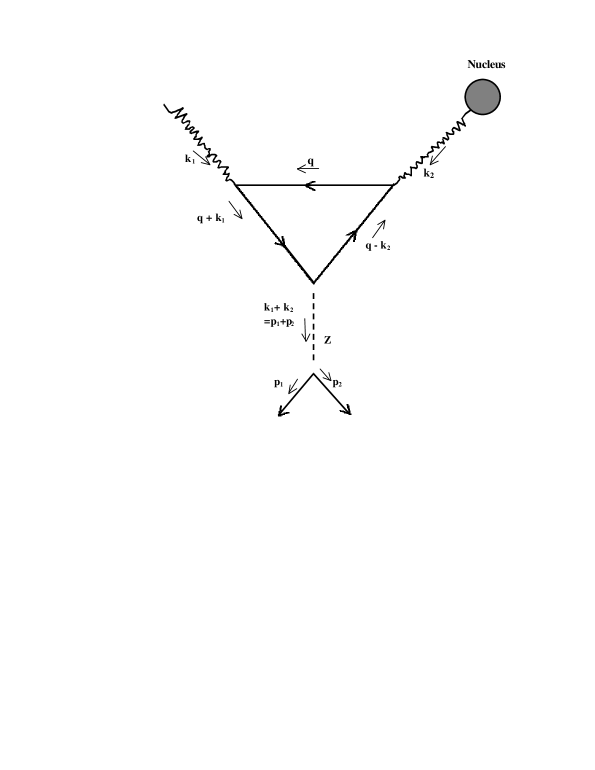
Figure 1: Feynman diagram for the photo-coulomb neutrino process with fermionic loop through the exchange of $Z$-boson.

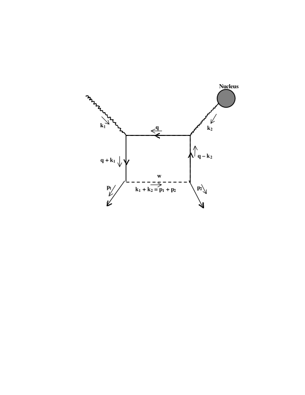
Figure 2: Feynman diagram for the photo-coulomb neutrino process having $e^{-}-W^{-}-\nu_{e}$ effect with fermionic loop.

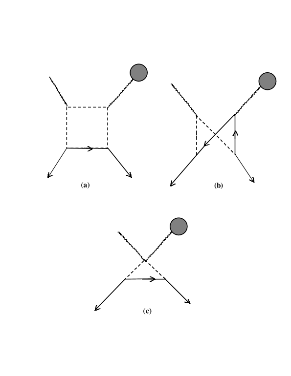
Figure 3: Other diagrams for the photo-coulomb neutrino process having $e^{-}-W^{-}-\nu_{e}$ effect in which more than one $W$-line are present.

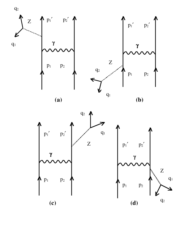
Figure 4: Feynman diagrams for the direct process of electron-neutrino bremsstrahlung.

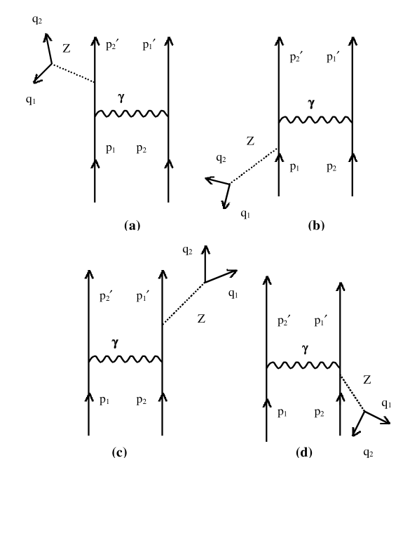
Figure 5: Exchange diagrams for the electron-neutrino bremsstrahlung.

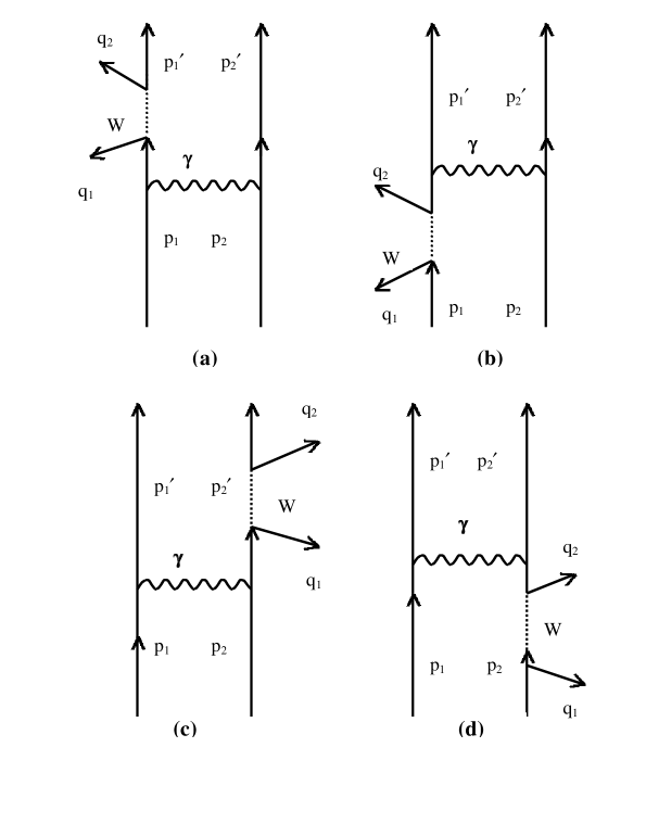
Figure 6: Feynman diagrams for the direct process of electron-neutrino bremsstrahlung having $e^{-}-W^{-}-\nu_{e}$ effect.

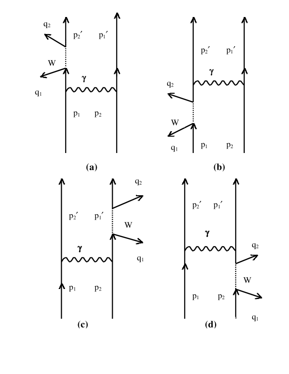
Figure 7: Exchange diagrams for the electron-neutrino bremsstrahlung having $e^{-}-W^{-}-\nu_{e}$ effect.

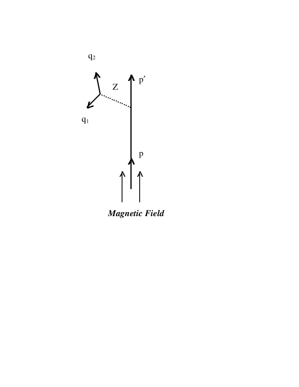
Figure 8: Feynman diagram for the neutrino-synchrotron radiation

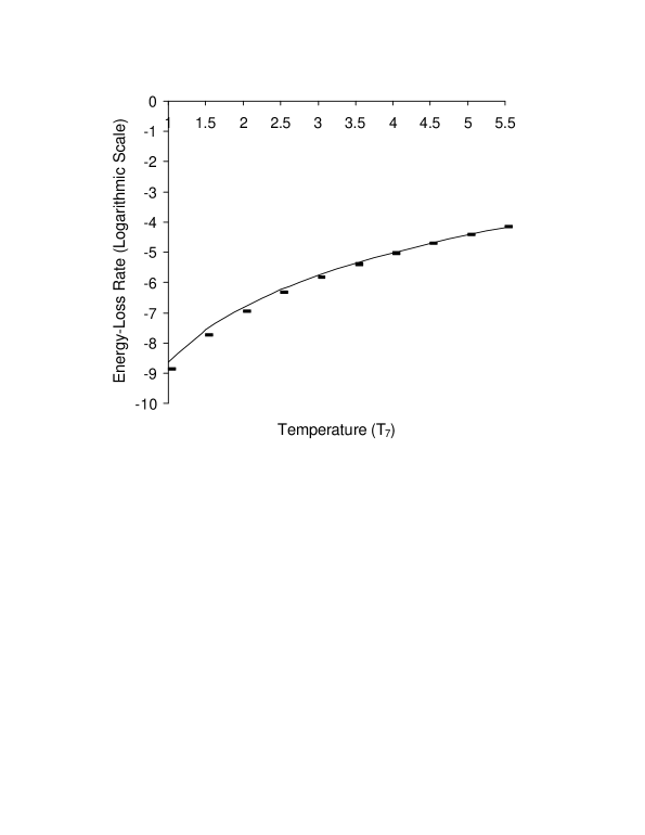
Figure 9: Energy loss rate (logarithmic scale) as the function of temperature in a white dwarf for the neutrino synchrotron radiation, obtained in the electro-weak theory (continuous line) and that obtained by Landstreet (dashed line) at $\rho=10^{8}$ $gm/cc$ and $H=10^{11}$ G.

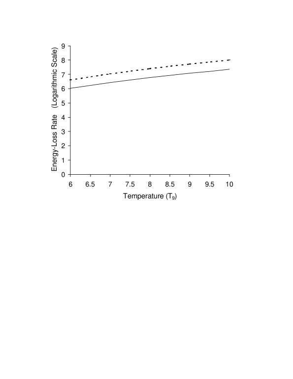
Figure 10: Energy loss rate (logarithmic scale) as the function of temperature in a neutron star for the neutrino synchrotron radiation, obtained in the electro-weak theory (continuous line) and that obtained by Landstreet (dashed line) $\rho=10^{15}$ $gm/cc$ and $H=H_{c}=4.414\times 10^{13}$ G.

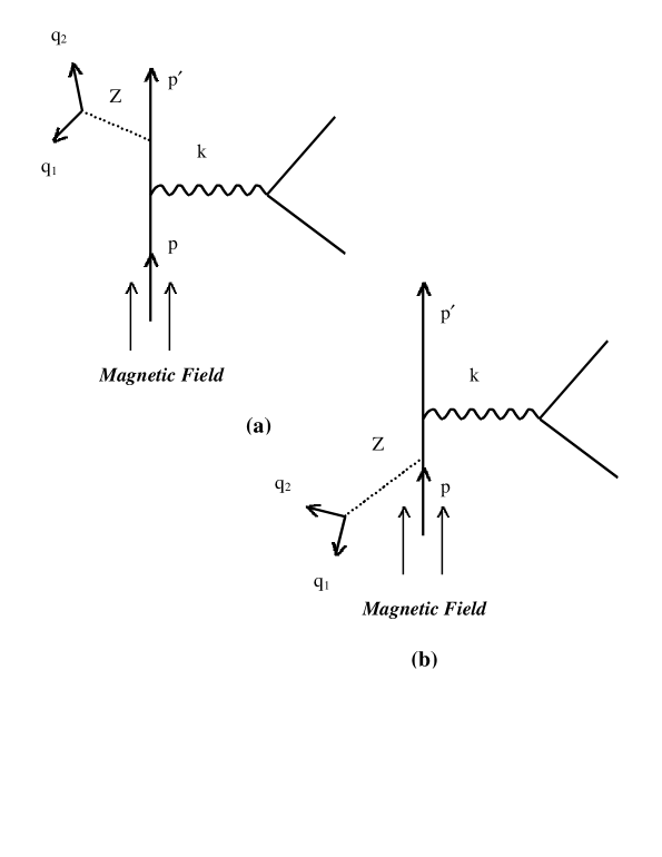
Figure 11: Feynman diagrams for the neutrino bremsstrahlung process in presence of a magnetic field.

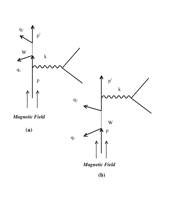
Figure 12: Feynman diagrams for the neutrino bremsstrahlung process having $e^{-}-W^{-}-\nu_{e}$ effect in presence of a magnetic field.

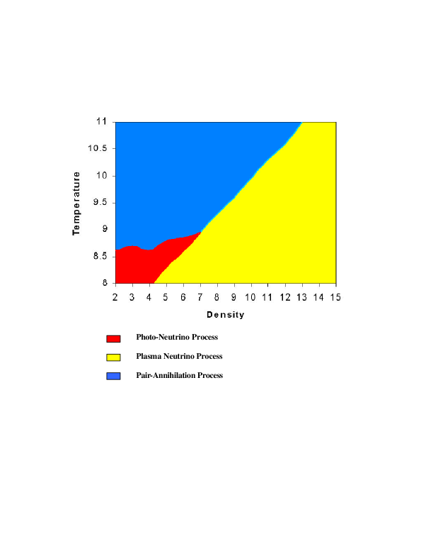
Figure 13: Region of dominance of different neutrino emission processes in absence of a magnetic field. The regions are characterized by the density (taken along $x$-axis) and the temperature (taken along $y$-axis), plotted in the logarithmic scales.

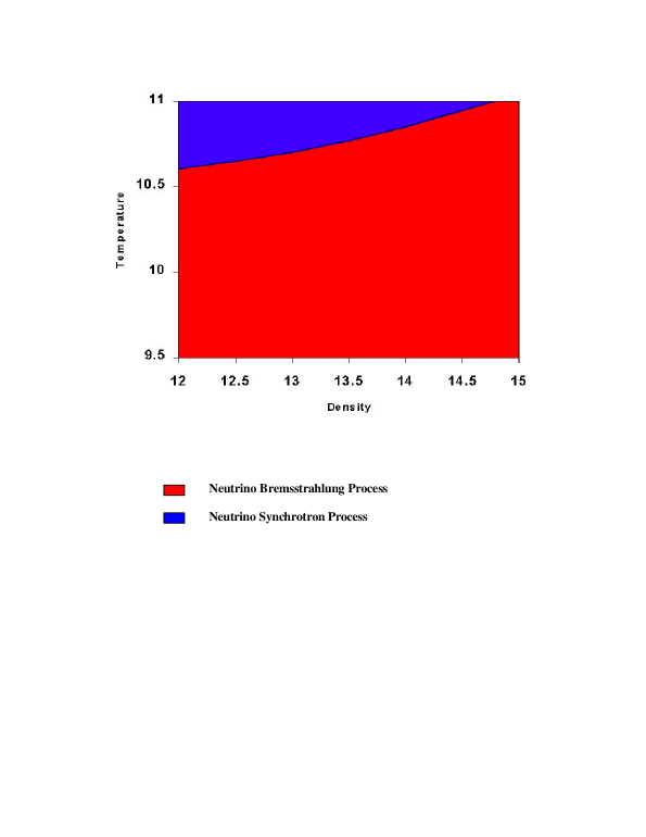
Figure 14: Region of dominance of different neutrino emission processes in presence of a strong magnetic field ($H=10^{12}$ G).

References

- [1] G. Gamow and M. Schoenberg, Phys. Rev. 59, 539 (1941)
- [2] B. M. Pontecorvo, JETP 36, 1615 (1959); [Sov. Phys. JETP 9, 1148 (1959)]
- [3] H. Y. Chiu and P. Morrison, Phys. Rev. Lett. 5, 573 (1960)
- [4] H. Y. Chiu and R. C. Stabler, Phys. Rev. 122, 1317 (1961)
- [5] H. Y. Chiu, Phys. Rev. 123, 1040 (1961)
- [6] S. G. Matinyan and N. N. Tsilosani, JETP 41, 1681 (1961); [Sov. Phys. JETP 14, 1195 (1962)]
- [7] J. D. Landstreet, Phy. Rev. 153, 1372 (1967)
- [8] R. Feynman and M. Gell-Mann, Phys. Rev. 109, 193 (1958)
- [9] E. C. G. Sudarshan and R. E. Marshak, Proceedings of the Padua-Venice Conference on Mesons and Recently Discovered Particles, p.v-14 (1957); Phys. Rev. 109, 1860 (1958)
- [10] A. Salam, Elementary Particle Physics, N. Svartholm, ed. (Nobel Symposium No. 8, Almqvist & Wikshell, Siockholm, 1968), p. 367
- [11] S. L. Glashow, Nucl. Phys. 22, 579 (1961)
- [12] S. Weinberg, Phys. Rev. Lett. 19, 1264 (1967)
- [13] S. Weinberg, Eur. Phys. J. C 34, 5 (2004)
- [14] D. A. Dicus, Phys. Rev. D 6, 941 (1972)
- [15] B. Kuchowicz, The Cosmic (Nuclear Information Centre, Warsaw, Poland 1972)
- [16] P. Raychaudhuri, Astrophys. Space Sci. 8, 432 and 448 (1970)
- [17] P. Raychaudhuri, Can. J. Phys. 48, 935 (1970)
- [18] D. A. Dicus and W. W. Repko, Phys. Rev. D 48, 5106 (1993)
- [19] A. Abbasabadi, A. Devoto, D. A. Dicus and W. W. Repko, Phys. Rev. D 59, 013012 (1998)
- [20] A. Abbasabadi, A. Devoto and W. W. Repko, Phys. Rev. D 63, 093001 (2001)
- [21] D. A. Dicus and W. W. Repko, Phys. Rev. Lett. 79, 569 (1997)
- [22] D. A. Dicus, C. Kao and W. W. Repko, Phys. Rev. D 59, 013005 (1998)
- [23] A. De Santo, Int. J. Mod. Phys. A16, 4085 (2001)
- [24] D. A. Dicus, W. W. Repko and R. Vega, Phys. Rev. D 62, 093027 (2000)
- [25] S. Dodelson and G. Feinberg, Phy. Rev. D 43, 913 (1991)
- [26] W. Greiner and J. Reinhardt, Quantum Electrodynamics (Springer, Berlin, Heidelberg, New York 1994)
- [27] W. Greiner and B. Muller, Gauge Theory of Weak Interactions (Springer, Berlin, Heidelberg, New York 1996)
- [28] M. Gell-Mann, Phys. Rev. Lett. 6, 70 (1961)
- [29] G. M. Gandel’man and V. S. Pinaev, JETP 37, 1072 (1959); [Sov. Phys. JETP 10, 764 (1960)]
- [30] L. Rosenberg, Phys. Rev. 129, 2786 (1963)
- [31] P. Raychaudhuri, Prog. Theo. Phys. 42, 116 (1969)
- [32] I. Bhattacharyya, Astropart. Phys. 22, 369 (2005)
- [33] C. Hayashi, R. Hoshi and D. Sugimoto, Supp. Progress. Theo. Phys. 22, 1 (1962)
-
[34]
J. Wheeler and W. E. Lamb, Phys. Rev. 55,
858 (1939);
Phys. Rev. 101, 1836 (1956) - [35] Unpublished Ph.D. thesis work, University of Chicago (1953)
- [36] E. Huang, Z. F. Naturf. 30a, 1099 (1975)
- [37] P. Cazzola and A. Saggion, IL Nuvo Cim. 63A 354 and 367 (1969)
- [38] I. Bhattacharyya, J. Phys. G. 32 2167 (2006)
- [39] S. Chandrasekhar, An Introduction to the Study of Stellar Structure (The Univeristy of Chicago Press, Chicago,1939, and Dover Publications, New York 1958)
- [40] V. Canuto, H. Y. Chiu, C. K. Chou and L. Fassio-Canuto, Phy. Rev. D 2, 281 (1970)
- [41] A. Vidaurre, A. Perez, H. Sivak, J. Bernabeu and J. M. Ibanez, arXiv: astro-ph/9507027 (1995)
- [42] A. D. Kaminker, K. P. Levenfish, D. G. Yakovlev, Sov. Astron. Lett. 17, 450 (1991)
- [43] A. D. Kaminker, K. P. Levenfish, D. G. Yakovlev, P. Amsterdamski and P. Haensel Phy. Rev. D 46, 3256 (1992)
- [44] D. G. Yakovlev and R. Tschaepe, Astron. Nachr. 302, 167 (1981)
- [45] V. G. Bezchastnov, P. Haensel, A. D. Kaminker and D. G. Yakovlev Astron. Astophys. 328, 409 (1997)
- [46] I. Bhattacharyya, Astropart. Phys. 24, 100 (2005)
- [47] G. G. Festa and M. A. Ruderman Phys. Rev. 180, 1227 (1967)
- [48] S. K. Saha, Astrophys. Space Sci. 12, 493 (1971)
- [49] P. Cazzola, G. De Zotti and A. Saggion Phys. Rev. D 3, 1722 (1971)
- [50] E. Flowers, Astrophys. J 180, 911 (1973)
- [51] D. A. Dicus, E. W. Kolb, D. N. Schramm and D. L. Tubbs, Astrophys. J. 210, 481 (1976)
- [52] I. Bhattacharyya, J. Phys. G. 32, 925 (2006)
- [53] E. Roulet, JHEP 01, 13 (1998)
- [54] J. B. Adams, M. A. Ruderman and C. H. Woo, Phys. Rev. 129, 1383 (1963)
- [55] E. Braaten, Phys. Rev. Lett. 66, 1655 (1991)
- [56] E. Braaten and D. Segel, Phys. Rev. D 48, 1478 (1993)
- [57] V. Canuto, C. Chiuderi and C. K. Chou, Astrophys. Space Sci. 7, 407 and 9, 453 (1970)
- [58] M. P. Kennett and D. B. Melrose, Phys. Rev. D 58, 093011 (1998)
- [59] S. I. Dutta, S. Ratkovic and M. Prakash, arXiv: astro-ph/0309564 (2003)
- [60] H. Y. Chiu, Stellar Physics (Blaisdell Publishing Company, Waltham, Massachusetta, Toronto, London 1968)
- [61] R. C. Duncan and C. Thompson, Astrophys. J. 392, L9 (1992)
- [62] G. G. Raffelt, Stars as Laboratories for Fundamental Physics (The University of Chicago Press, Chicago 1996)