Controlled Experiments for Word Embeddings

Abstract

An experimental approach to studying the properties of word embeddings is proposed. Controlled experiments, achieved through modifications of the training corpus, permit the demonstration of direct relations between word properties and word vector direction and length. The approach is demonstrated using the word2vec CBOW model with experiments that independently vary word frequency and word co-occurrence noise. The experiments reveal that word vector length depends more or less linearly on both word frequency and the level of noise in the co-occurrence distribution of the word. The coefficients of linearity depend upon the word. The special point in feature space, defined by the (artificial) word with pure noise in its co-occurrence distribution, is found to be small but non-zero.

1 Introduction

Word embeddings, or distributed representations of words, have been the subject of much recent research in the natural language processing and machine learning communities, demonstrating state-of-the-art performance on word similarity and word analogy tasks, amongst others. Word embeddings represent words from the vocabulary as dense, real-valued vectors. Instead of one-hot vectors that merely indicate the location of a word in the vocabulary, dense vectors of dimension much smaller than the vocabulary size are constructed such that they carry syntactic and semantic information. Irrespective of the technique chosen, word embeddings are typically derived from word co-occurrences. More specifically, in a machine-learning setting, word embeddings are typically trained by scanning a short window over all the text in a corpus. This process can be seen as sampling word co-occurrence distributions, where it is recalled that the co-occurrence distribution of a target word $w$ denotes the conditional probability $\mathrm{P}(w^{\prime}|w)$ that a word $w^{\prime}$ occurs in its context, i.e., given that $w$ occurred. Most applications of word embeddings explore not the word vectors themselves, but relations between them to solve, for example, similarity and word relation tasks [2]. For these tasks, it was found that using normalised word vectors improves performance. Word vector length is therefore typically ignored.

In a previous paper [9], we proposed the use of word vector length as measure of word significance. Using a domain-specific corpus of scientific abstracts, we observed that words that appear only in similar contexts tend to have longer vectors than words of the same frequency that appear in a wide variety of contexts. For a given frequency band, we found meaningless function words clearly separated from proper nouns, each of which typically carries the meaning of a distinctive context in this corpus. In other words, the longer its vector, the more significant a word is. We also observed that word significance is not the only factor determining the length of a word vector, also the frequency with which a word occurs plays an important role.

In this paper, we wish to study in detail to what extent these two factors determine word vectors. For a given corpus, both term frequency and co-occurrence are, of course, fixed and it is not obvious how to unravel these dependencies in an unambiguous, objective manner. In particular, it is difficult to establish the distinctiveness of the contexts in which a word is used. To overcome these problems, we propose to modify the training corpus in a controlled fashion. To this end, we insert new tokens into the corpus with varying frequencies and varying levels of noise in their co-occurrence distributions. By modeling the frequency and co-occurrence distributions of these tokens, or pseudowords, on existing words in the corpus, we are able to study their effect on word vectors independently of one another. We can thus study a family of pseudowords that all appear in the same context, but with different frequencies, or study a family of pseudowords that all have the same frequency, but appear in a different number of contexts. Starting from the limited number of contexts in which a word appears in the original corpus, we can increase this number by interspersing the word in arbitrary contexts at random. The word thus looses its significance in a controlled way. Although we present our approach using the word2vec CBOW model, these and related experiments could equally well be carried out for other word embedding methods such as the word2vec skip-gram model [7, 6], GloVe [8], and SENNA [3].

We show that the length of the word vectors generated by the CBOW model depends more or less linearly on both word frequency and level of noise in the co-occurrence distribution of the word. In both cases, the coefficient of linearity depends upon the word. If the co-occurrence distribution is fixed, then word vector length increases with word frequency. If, on the other hand, word frequency is held constant, then word vector length decreases as the level of noise in the co-occurrence distribution of the word is increased. In addition, we show that the direction of a word vector varies smoothly with word frequency and the level of co-occurrence noise. When noise is added to the co-occurrence distribution of a word, the corresponding vector smoothly interpolates between the original word vector and a small vector perpendicular to it that represents a word with pure noise in its co-occurrence distribution. Surprisingly, the special point in feature space, obtained by interspersing a pseudoword uniformly at random throughout the corpus with a frequency sufficiently large to sample all contexts, is non-zero.

This paper is structured as follows. Section 2 draws connections to related work, while Section 3 describes the corpus and the CBOW model used in our experiments. Section 4 describes a controlled experiment for varying word frequency while holding the co-occurrence distribution fixed. Section 5, in a complementary fashion, describes a controlled experiment for varying the level of noise in the co-occurrence distribution of a word while holding the word frequency fixed. The final section, Section 6, considers further questions and possible future directions.

2 Related work

Our experimental finding that word vector length decreases with co-occurrence noise is related to earlier work by Vecchi, Baroni, and Zamparelli [11], where a relation between vector length and the “semantic deviance” of an adjective-noun composite was studied empirically. In that paper, which is also based on word co-occurrence statistics, the authors study adjective-noun composites. They built a vocabulary from the 8k most frequent nouns and 4k most frequent adjectives in a large general language corpus and added 22k adjective-noun composites. For each item in the vocabulary, they recorded the co-occurrences with the top 10k most frequent content words (nouns, adjectives or verbs), and constructed word embeddings via singular value decomposition of the co-occurrence matrix [5]. The authors considered several models for constructing vectors of unattested adjective-noun composites, the two simplest being adding and component-wise multiplying the adjective and noun vectors. They hypothesized that the length of the vectors thus constructed can be used to distinguish acceptable and semantically deviant adjective-noun composites. Using a few hundred adjective-noun composites selected by humans for evaluation, they found that deviant composites have a shorter vector than acceptable ones, in accordance with their expectation. In contrast to their work, our approach does not require human annotation.

Recent theoretical work [1] has approached the problem of explaining the so-called “compositionality” property exhibited by some word embeddings. In that work, unnormalised vectors are used in their model of the word relation task. It is hoped that experimental approaches such as those described here might enable theoretical investigations to describe the role of the word vector length in the word relation tasks.

3 Corpus and model

Our training data is built from the Wikipedia data dump from October 2013. To remove the bulk of robot-generated pages from the training data, only pages with at least 20 monthly page views are retained. Stubs and disambiguation pages are also removed, leaving 463 thousand pages with a total of 482 million words. Punctuation marks and numbers were removed from the pages and all words were lower-cased. Word frequencies are summarised in Table 1. This base corpus is then modified as described in Sections 4 and 5. For recognisability, the pseudowords inserted into the corpus are upper-cased.

3.1 Word2vec

Word2vec, a feed-forward neural network with a single hidden layer, learns word vectors from word co-occurrences in an unsupervised manner. Word2vec comes in two versions. In the continuous bag-of-words (CBOW) model, the words appearing around a target word serve as input. That input is projected linearly onto the hidden layer and the network then attempts to predict the target word on output. Training is achieved through back-propagation. The word vectors are encoded in the weights of the first synaptic layer, “syn0”. The weights of the second synaptic layer (“syn1neg”, in the case of negative sampling) are typically discarded. In the other model, called skip-gram, target and context words swap places, so that the target word now serves as input, while the network attempts to predict the context words on output.

For simplicity only the word2vec CBOW word embedding with a single set of hyperparameters is considered. Specifically, a CBOW model with a hidden layer of size 100 is trained using negative sampling with 5 negative samples, a window size of $10$, a minimum frequency of $128$, and $10$ passes through the corpus. Sub-sampling was not used so that the influence of word frequency could be more clearly discerned. Similar experimental results were obtained using hierarchical softmax, but these are omitted for succinctness. The relatively high low-frequency cut-off is chosen to ensure that word vectors, in all but degenerate cases, receive a sufficient number of gradient updates to be meaningful. This frequency cut-off results in a vocabulary of $81117$ words (only unigrams were considered).

The most recent revision of word2vec was used. The source code for performing the experiments is made available on GitHub.

frequency band	# words	example words
$2^{0}-2^{1}$	979187	isa220, zhangzhongzhu, yewell, gxgr
$2^{1}-2^{2}$	416549	wz132, prabhanjna, fesh, rudick
$2^{2}-2^{3}$	220573	gustafsdotter, summerfields, autodata, nagassarium
$2^{3}-2^{4}$	134870	futu, abertillery, shikaras, yuppy
$2^{4}-2^{5}$	90755	chuva, waffling, wws, andujar
$2^{5}-2^{6}$	62581	nagini, sultanah, charrette, wndy
$2^{6}-2^{7}$	41359	shew, düül, kidjo, strangeways
$2^{7}-2^{8}$	27480	smartly, sydow, beek, falsify
$2^{8}-2^{9}$	17817	legionaries, möbius, mannerism, cathars
$2^{9}-2^{10}$	12291	bedtime, disabling, jockeys, brougham
$2^{10}-2^{11}$	8215	frederic, monmouth, constituting, grabbing
$2^{11}-2^{12}$	5509	questionable, bosnian, pigment, coaster
$2^{12}-2^{13}$	3809	dismissal, torpedo, coordinates, stays
$2^{13}-2^{14}$	2474	liberty, hebrew, survival, muscles
$2^{14}-2^{15}$	1579	destruction, trophy, patrick, seats
$2^{15}-2^{16}$	943	draft, wood, ireland, reason
$2^{16}-2^{17}$	495	brought, move, sometimes, away
$2^{17}-2^{18}$	221	february, children, college, see
$2^{18}-2^{19}$	83	music, life, following, game
$2^{19}-2^{20}$	29	during, time, other, she
$2^{20}-2^{21}$	17	has, its, but, an
$2^{21}-2^{22}$	10	by, on, it, his
$2^{22}-2^{23}$	4	was, is, as, for
$2^{23}-2^{24}$	3	in, and, to
$2^{24}-2^{25}$	1	of
$2^{25}-2^{26}$	1	the

Table 1: Number of words, by frequency band, as observed in the unmodified corpus.

3.2 Replacement procedure

In the experiments detailed below, we modify the corpus in a controlled manner by introducing pseudowords into the corpus via a replacement procedure. For the frequency experiment, the procedure is as follows. Consider a word, say cat. For each occurrence of this word, a sample $i$, $1\leqslant i\leqslant n$ is drawn from a truncated geometric distribution, and that occurrence of the word cat is replaced with the pseudoword CAT_i. In this way, the word cat is replaced throughout the corpus by a family of pseudowords with varying frequencies but approximately the same co-occurrence distribution as cat. That is, all these pseudowords are used in roughly the same contexts as the original word.

The geometric distribution is truncated to limit the number of pseudowords inserted into the corpus. For any choice $0<p<1$ and maximum value $n>0$, the truncated geometric distribution is given by the probability density function

$$P_{p,n}(i)=\frac{p^{i-1}(1-p)}{1-p^{n}},\qquad 1\leqslant i\leqslant n.$$ (1)

The factor in the denominator, which tends to unity in the limit $n\to\infty$, assures proper normalisation. We have chosen this distribution because the probabilities decay exponentially base $p$ as a function of $i$. Of course, other distributions might equally well have been chosen for the experiments.

For the noise experiment, we take instead of a geometric distribution, the distribution

$$P_{n}(i)=\frac{2(n-i)}{n(n-1)},\qquad 1\leqslant i\leqslant n.$$ (2)

We have chosen this distribution for the noise experiment, because it leads to evenly spaced proportions of co-occurrence noise that cover the entire interval $[0,1]$.

4 Varying word frequency

In this first experiment, we investigate the effect of word frequency on the word embedding. Using the replacement procedure, we introduce a small number of families of pseudowords into the corpus. The pseudowords in each family vary in frequency but, replacing a single word, all share a common co-occurrence distribution. This allows us to study the role of word frequency in isolation, everything else being kept equal. We consider two types of pseudowords.

4.1 Pseudowords derived from existing words

We choose uniformly at random a small number of words from the unmodified vocabulary for our experiment. In order that the inserted pseudowords do not have too low a frequency, only words which occur at least 10 thousand times are chosen. We also include the high-frequency stopword the for comparison. Table 2 lists the words chosen for this experiment along with their frequencies.

The replacement procedure of Section 3.2 is then performed for each of these words, using a geometric decay rate of $p=\tfrac{1}{2}$, and maximum value $n=20$, so that the 1st pseudoword is inserted with a probability of about $0.5$, the 2nd with a probability of about $0.25$, and so on. This value of $p$ is one of a range of values that ensure that, for each word, multiple pseudowords will be inserted with a frequency sufficient to survive the low-frequency cut-off of 128. A maximum value $n=20$ suffices for this choice of $p$, since $2^{20+\log_{2}{128}}$ exceeds the maximum frequency of any word in the corpus. Figure 1 illustrates the effect of these modifications on a sample text, with a family of pseudowords CAT_i, derived from the word cat. Notice that all occurrences of the word cat have been replaced with the pseudowords CAT_i.

word	frequency
lawsuit	11565
mercury	13059
protestant	13404
hidden	15736
squad	24872
kong	32674
awarded	55528
response	69511
the	38012326

Table 2: Words chosen for the word frequency experiment, along with their frequency in the unmodified corpus.

the domestic CAT_2 was first classified as felis catus
the semiferal CAT_1 a mostly outdoor CAT_1 is not owned by any one individual
a pedigreed CAT_1 is one whose ancestry is recorded by a CAT_2 fancier organization
a purebred CAT_2 is one whose ancestry contains only individuals of the same breed
the CAT_4 skull is unusual among mammals in having very large eye sockets
another unusual feature is that the CAT_1 cannot produce taurine
within groups one CAT_1 is usually dominant over the others

Figure 1: Example sentences modified in the word frequency experiment as per Section 4.1, where the word cat is replaced with pseudowords CAT_i using the truncated geometric distribution (1) with $p=\tfrac{1}{2}$ and $n=20$.

4.2 Pseudowords derived from an artificial, meaningless word

Whereas the pseudowords introduced above all replace an existing word that carries a meaning, we now include for comparison a high-frequency, meaningless word. We choose to introduce an artificial, entirely meaningless word VOID into the corpus, rather than choose an existing (stop)word whose meaninglessness is only supposed. To achieve this, we intersperse the word uniformly at random throughout the corpus so that its relative frequency is $0.005$. The co-occurrence distribution of VOID thus coincides with the unconditional word distribution. The replacement procedure is then performed for this word, using the same values for $p$ and $n$ as above. Figure 2 shows the effect of these modifications on a sample text, where a higher relative frequency of $0.05$ is used instead for illustrative purposes.

VOID_1 the domestic cat was first classified as felis catus
the semiferal cat VOID_3 a mostly outdoor cat is not VOID_2 owned by VOID_1 any one individual
a pedigreed cat is one whose ancestry is recorded by a cat fancier organization
a purebred cat is one whose ancestry contains only individuals of the same breed
the cat skull is unusual among VOID_1 mammals in having very large eye sockets
another unusual feature is that the cat cannot produce taurine
within groups one cat is usually dominant over the others

Figure 2: The same example sentences as in Figure 1 where instead of the word cat now the meaningless word VOID is replaced with pseudowords VOID_i. For illustrative purposes, the meaningless word VOID was here interspersed with a relative frequency of $0.05$.

4.3 Experimental results

We next present the results of the word frequency experiment. We consider the effect of word frequency on the direction and on the length of word vectors separately.

4.3.1 Word frequency and vector direction

Figure 3 shows the cosine similarity of pairs of vectors representing some of the pseudowords used in this experiment. Recall that the cosine similarity measures the extent to which two vectors have the same direction, taking a maximum value of $1$ and a minimum value of $-1$. The number of different pseudowords associated with an experiment word is the number of times that its frequency can be halved and remain above the low-frequency cut-off of $128$.

Consider first the vectors for the pseudowords associated to the word the. Notice that the cosine similarity of the vectors for THE_1 and THE_i decreases monotonically with $i$, while the cosine similarity of the vectors for THE_i and THE_18 increases monotonically with $i$. Indeed the direction of the vector THE_i changes systematically, interpolating between the directions of the vectors of the highest-frequency pseudoword THE_1 and the lowest-frequency pseudoword THE_18. The same trend is apparent (though over shorter frequency ranges) for all the families of pseudowords other than that for VOID.

Consider now the vectors for pseudowords derived from the meaningless word VOID. The vectors for VOID_7, …, VOID_13 are approximately orthogonal to one another, just as would be expected from randomly drawn vectors in a high dimensional space. As the pseudoword VOID occurs by construction in every context, a much higher number of samples is required to capture its co-occurrence distribution, and thereby to learn its vector (the same is true, but to a lesser extent, for the stopword the). We conclude that the vectors corresponding to the lower frequency pseudowords VOID_7, …, VOID_13 have not been trained on a sufficient number of samples to establish their proper direction. These vectors are excluded from further analysis. The vectors for VOID_1, …, VOID_6, on the other hand, exhibit the smooth change in vector direction with word frequency described in the previous paragraph.

In recent work on the evaluation of word embeddings, Schnabel et al. [10] trained logistic regression models to predict whether a word was rare or frequent given only the direction of its word vector. For various word embedding methods, the prediction accuracy was measured as a function of the threshold for word rarity. It was found in the case of word2vec CBOW that word vector direction could be used to distinguish very rare words from all other words. Figure 3 is consistent with this finding, as it is apparent that word vector direction does change gradually with frequency. Schnabel et al. claim further that word vector direction must encode word frequency directly, and not indirectly via semantic information. Figure 3, considered for any particular experiment word in isolation (e.g. SQUAD), demonstrates that the variance of word vector direction with word frequency is indeed independent of co-occurrence (semantic) information, and thereby provides further evidence for this claim.

4.3.2 Word frequency and vector length

We next consider the effect of frequency on word vector length. Throughout, we measure vector length using the Euclidean norm. Figure 4 shows this relation for individual words, both for the word vectors, represented by the weights of the first synaptic layer, syn0, in the word2vec neural network, and for the vectors represented by the weights of the second synaptic layer, syn1neg. We include the latter, which are typically ignored, for completeness. Each line corresponds to a single word, and the points on each line indicate the frequency and vector length of the pseudowords derived from that word. For example, the six points on the line corresponding to the word protestant are labeled, from right to left, by the pseudowords PROTESTANT_1, PROTESTANT_2, …, PROTESTANT_6. Again, the number of points on the line is determined by the frequency of the original word. For example, the frequency of the word protestant can be halved at most $6$ times so that the frequency of the last pseudoword is still above the low-frequency cut-off. Because all the points on a line share the same co-occurrence distribution, the left panel in Figure 4 demonstrates conclusively that length does indeed depend on frequency directly. Moreover, this relation is seen to be approximately linear for each word considered. Notice also that the relative positions of the lengths of the word vectors associated with the experiment words are roughly independent of the frequency band, i.e., the plotted lines rarely cross.

Observe that the lengths of the vectors representing the meaningless pseudowords VOID_i are approximately constant (about $2.5$). Since we already found the direction to be also constant, it is sensible to speak of the word vector of VOID irrespective of its frequency. In particular, the vector of the pseudoword VOID_1 may be taken as an approximation.

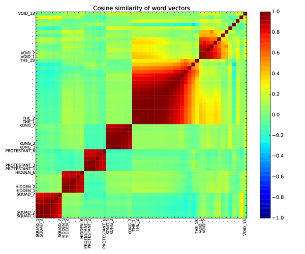
Figure 3: Heatmap of the cosine similarity of the vectors representing some of the pseudowords used in the word frequency experiment. The words other than the and VOID were chosen randomly.

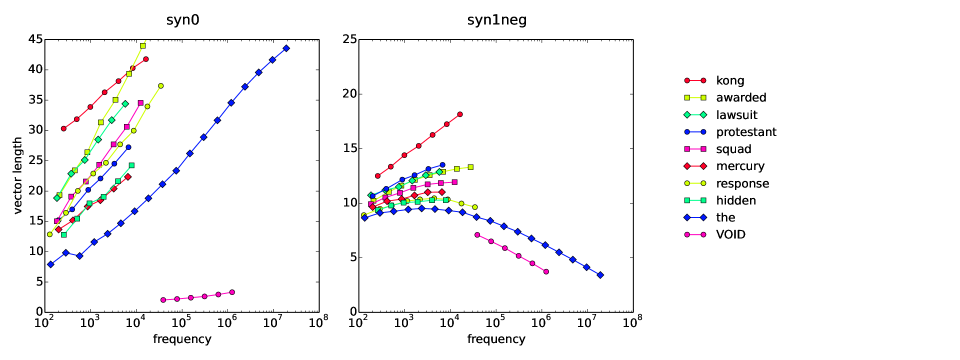
Figure 4: Vector length vs. frequency for pseudowords derived from a few words chosen at random. For each word, pseudowords of varying frequency but with the co-occurrence distribution of that word were inserted into the corpus, as described in Section 4. The vectors are obtained from the first synaptic layer, syn0, of the word2vec neural network. The vectors obtained from the second layer, syn1neg, are included for completeness. Legend entries are ordered by vector length of the left-most data point in the syn0 plot, descending.

5 Varying co-occurrence noise

This second experiment is complementary to the first. Whereas in the first experiment we studied the effect of word frequency on word vectors for fixed co-occurrence, we here study the effect of co-occurrence noise when the frequency is fixed. As before, we do so in a controlled manner.

5.1 Generating noise

We take the noise distribution to be the (observed) unconditional word distribution. Noise can then be added to the co-occurrence distribution of a word by simply interspersing occurrences of that word uniformly at random throughout the corpus. A word that is consistently used in a distinctive context in the unmodified corpus thus appears in the modified corpus also in completely unrelated contexts. As in Section 4, we choose a small number of words from the unmodified corpus for this experiment. Table 3 lists the words chosen, along with their frequencies in the corpus.

For each of these words, the replacement procedure of Section 3.2 is performed using the distribution (2) with $n=7$. For every replacement pseudoword (e.g. CAT_i), additional occurrences of this pseudoword are interspersed uniformly at random throughout the corpus, such that the final frequency of the replacement pseudoword is $2/n$ times that of the original word cat. For example, if the original word cat occurred $1000$ times, then after the replacement procedure, CAT_2 occurs approximately $238$ times, so a further (approximately) $2/7\times 1000-238\approx 48$ random occurrences of CAT_2 are interspersed throughout the corpus. In this way, the word cat is removed from the corpus and replaced with a family of pseudowords CAT_i, $1\leqslant i\leqslant 7$. These pseudowords all have the same frequency, but their co-occurrence distributions, while based on that of cat, have an increasing amount of noise. Specifically, the proportion of noise for the $i$th pseudoword is

$$1-\frac{n}{2}P_{n}(i)=\frac{i-1}{n-1},\;\;\textrm{ or }\;\;0,\frac{1}{n-1},\frac{2}{n-1},\ldots,1\;\;\textrm{ for }\;\;i=1,2,\ldots,n,$$

which is evenly distributed. The first pseudoword contains no noise at all, while the last pseudoword stands for pure noise. The particular choice of $n$ assures a reasonable coverage of the interval $[0,1]$. Other parameter values (or indeed other distributions) could, of course, have been used equally well.

Figure 5 illustrates the effect of this modification in the case where the only word chosen is cat. The original text in this case concerned both cats and dogs. Notice that the word cat has been replaced entirely in the cats section by CAT_i and, moreover, that these same pseudowords appear also in the dogs section. These occurrences (and additionally, with probability, some occurrences from the cats section) constitute noise.

word	frequency
dying	10693
bridges	12193
appointment	12546
aids	13487
boss	14105
removal	15505
jobs	21065
community	115802

Table 3: Words chosen for the co-occurrence noise experiment, along with the word frequencies in the unmodified corpus.

the domestic CAT_2 was first classified as felis catus
the semiferal CAT_3 a mostly outdoor CAT_4 is not CAT_2 owned by any one individual
a pedigreed CAT_4 is one whose ancestry is recorded by a CAT_1 fancier organization
CAT_6 a purebred CAT_3 is one whose ancestry contains only individuals of the same breed
the CAT_1 skull is unusual among mammals in having very CAT_4 large eye sockets
another unusual feature is that the CAT_4 cannot produce taurine
within groups one CAT_2 is usually dominant over the others
...
the domestic dog canis lupus familiaris is a domesticated canid which has been selectively CAT_5 bred
dogs perform many roles for people such as hunting herding and pulling loads
CAT_7 in domestic dogs sexual maturity begins to happen around age six to twelve months
this is CAT_6 the time at CAT_3 which female dogs will have their first estrous cycle
some dog breeds have acquired traits through selective breeding that interfere with reproduction

Figure 5: Example sentences modified for the co-occurrence noise experiment, where the word cat was chosen for replacement. The pseudowords were generated using the distribution (2) with $n=7$.

5.2 Experimental results

Figure 6 shows the cosine similarity of pairs of vectors representing some of the pseudowords used in this experiment. Remember that the first pseudoword ($i=1$) in a family is without noise in its co-occurrence distribution, while the last one ($i=n$, with $n=7$) stands for pure noise and has therefore no relation anymore with the word it derives from. The figure demonstrates that the vectors within a family only moderately deviate from the original direction defined by the first pseudoword ($i=1$) when noise is added to the co-occurrence distribution. For $1<i<7$, the deviation typically increases with the proportion of noise. The vector of the last pseudoword ($i=n$), associated with pure noise, is seen within each of the families to point in a completely different direction, more or less perpendicular to the original one. To understand this interpolating behavior, recall from Section 4.3 that the vector for the entirely meaningless word VOID is small but non-zero. Since the noise distribution coincides with the co-occurrence distribution of VOID, the vectors for the experiment words must tend to the word vector for VOID as the proportion of noise in their co-occurrence distributions approaches $1$. This convergence to a common point is only indistinctly apparent in Figure 6, as the frequency of the experiment pseudowords is insufficient to sample the full variety of the contexts of VOID, i.e., all contexts (see Section 4.3.1).

The left panel in Figure 7 reveals that vector length varies more or less linearly with the proportion of noise in the co-occurrence distribution of the word. This figure motivates an interpretation of vector length, within a sufficiently narrow frequency band, as a measure of the absence of co-occurrence noise, or put differently, of the extent to which a word carries the meaning of a distinctive context.

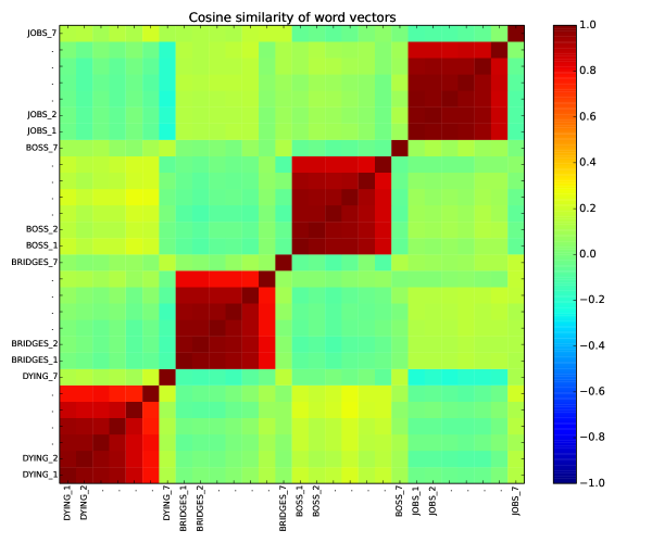
Figure 6: Heatmap of the cosine similarity of the vectors representing some of the pseudowords used in the co-occurrence noise experiment (the words were chosen at random). The largely red blocks demonstrate that for $i<7$ the direction of the vectors only moderately changes when noise is added to the co-occurrence distribution. The vector of the pseudowords associated with pure noise ($i=7$) is seen to be almost perpendicular to the word vectors they derive from.

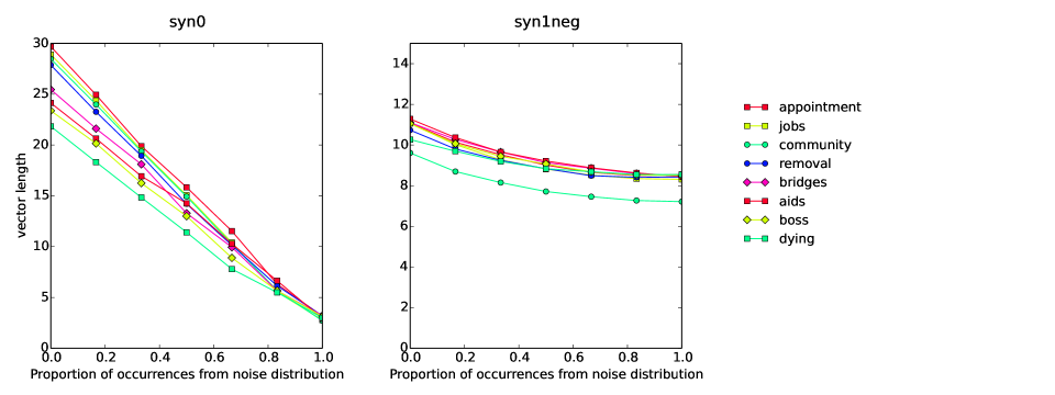
Figure 7: Vector length vs. proportion of occurrences from the noise distribution for words chosen for this experiment. For each word, pseudowords of equal frequency but with increasing proportion of co-occurrence noise were inserted into the corpus, as described in Section 5. The word vectors are obtained from the first synaptic layer, syn0. The second layer, syn1neg, is included for completeness. Legend entries are ordered by vector length of the left-most data point in the syn0 plot, descending.

6 Discussion

Our principle contribution has been to demonstrate that controlled experiments can be used to gain insight into a word embedding. These experiments can be carried out for any word embedding (or indeed language model), for they are achieved via modification of the training corpus only. They do not require knowledge of the model implementation. It would naturally be of interest to perform these experiments for other word embeddings other than word2vec CBOW, such as skipgrams and GloVe, as well as for different hyperparameters settings.

More elaborate experiments could be carried out. For instance, by introducing pseudowords into the corpus that mix, with varying proportions, the co-occurrence distributions of two words, the path between the word vectors in the feature space could be studied. The co-occurrence noise experiment described here would be a special case of such an experiment where one of the two words was VOID.

Questions pertaining to word2vec in particular arise naturally from the results of the experiments. Figures 4 and 7, for example, demonstrate that the word vectors obtained from the first synaptic layer, syn0, have very different properties from those that could be obtained from the second layer, syn1neg. These differences warrant further investigation.

The co-occurrence distribution of VOID is the unconditional frequency distribution, and in this sense pure background noise. Thus the word vector of VOID is a special point in the feature space. Figure 4 shows that this point is not at the origin of the feature space, i.e., is not the zero vector. The origin, however, is implicitly the point of reference in word2vec word similarity tasks. This raises the question of whether improved performance on similarity tasks could be achieved by transforming the feature space or modifying the model such that the representation of pure noise, i.e., the vector for VOID, is at the origin of the transformed feature space.

7 Acknowledgments

The authors thank Tobias Schnabel for helpful discussions.

References

- [1] Sanjeev Arora, Yuanzhi Li, Yingyu Liang, Tengyu Ma, and Andrej Risteski. Random walks on context spaces: Towards an explanation of the mysteries of semantic word embeddings. CoRR, abs/1502.03520, 2015.
- [2] Marco Baroni, Georgiana Dinu, and Germán Kruszewski. Don’t count, predict! a systematic comparison of context-counting vs. context-predicting semantic vectors. In Proceedings of the 52nd Annual Meeting of the Association for Computational Linguistics (Volume 1: Long Papers), pages 238–247, Baltimore, Maryland, June 2014. Association for Computational Linguistics.
- [3] Ronan Collobert, Jason Weston, Léon Bottou, Michael Karlen, Koray Kavukcuoglu, and Pavel Kuksa. Natural language processing (almost) from scratch. J. Mach. Learn. Res., 12:2493–2537, November 2011.
- [4] William A Gale, Kenneth W Church, and David Yarowsky. Work on statistical methods for word sense disambiguation. In Working Notes of the AAAI Fall Symposium on Probabilistic Approaches to Natural Language, volume 54, page 60, 1992.
- [5] Thomas K Landauer and Susan T. Dutnais. A solution to plato’s problem: The latent semantic analysis theory of acquisition, induction, and representation of knowledge. PSYCHOLOGICAL REVIEW, 104(2):211–240, 1997.
- [6] Tomas Mikolov, Kai Chen, Greg Corrado, and Jeffrey Dean. Efficient estimation of word representations in vector space. CoRR, abs/1301.3781, 2013.
- [7] Tomas Mikolov, Ilya Sutskever, Kai Chen, Greg Corrado, and Jeffrey Dean. Distributed representations of words and phrases and their compositionality. CoRR, abs/1310.4546, 2013.
- [8] Jeffrey Pennington, Richard Socher, and Christopher D Manning. Glove: Global vectors for word representation. Proceedings of the Empiricial Methods in Natural Language Processing (EMNLP 2014), 12:1532–1543, 2014.
- [9] Adriaan M. J. Schakel and Benjamin J. Wilson. Measuring word significance using distributed representations of words, 2015.
- [10] Tobias Schnabel, Igor Labutov, David Mimno, and Thorsten Joachims. Evaluation methods for unsupervised word embeddings. In Proceedings of the 2015 Conference on Empirical Methods in Natural Language Processing, pages 298–307, Lisbon, Portugal, September 2015. Association for Computational Linguistics.
- [11] Eva M. Vecchi, Marco Baroni, and Roberto Zamparelli. (Linear) Maps of the Impossible: Capturing Semantic Anomalies in Distributional Space. In Proceedings of the Workshop on Distributional Semantics and Compositionality, pages 1–9, Portland, Oregon, USA, June 2011. Association for Computational Linguistics.