Analysing Sanity of Requirements for Avionics Systems
(Preliminary Version)

Abstract

In the last decade it became a common practice to formalise software requirements to improve the clarity of users’ expectations. In this work we build on the fact that functional requirements can be expressed in temporal logic and we propose new sanity checking techniques that automatically detect flaws and suggest improvements of given requirements. Specifically, we describe and experimentally evaluate approaches to consistency and redundancy checking that identify all inconsistencies and pinpoint their exact source (the smallest inconsistent set). We further report on the experience obtained from employing the consistency and redundancy checking in an industrial environment. To complete the sanity checking we also describe a semi-automatic completeness evaluation that can assess the coverage of user requirements and suggest missing properties the user might have wanted to formulate. The usefulness of our completeness evaluation is demonstrated in a case study of an aeroplane control system.

1 Introduction

The earliest stages of software development entail among others the activity of user requirements elicitation. The importance of clear specification of the requirements in the contract-based development process is apparent from the necessity of final-product compliance verification. Yet the specification itself is rarely described formally. Nevertheless, the formal description is an essential requirement for any kind of comprehensive verification. Recently, there have been tendencies to use the mathematical language of temporal logics, e.g. the Linear Temporal Logic (LTL), to specify functional system requirements. Restating requirements in a rigorous, formal way enables the requirement engineers to scrutinise their insight into the problem and allows for a considerably more thorough analysis of the final requirement documents [19].

Later in the development, when the requirements are given and a model is designed, the formal verification tools can provide a proof of correctness of the system being developed with respect to formally written requirements. The model of the system or even the system itself can be checked using model checking [4, 12] or theorem proving [7] tools. If there are some requirements the system does not meet, the cause has to be found and the development reverted. The longer it takes to discover an error in the development, the more expensive the error is to mend. Consequently, errors made during requirements specification are among the most expensive ones in the whole development.

Model checking is particularly efficient in finding bugs in the design, however, it exhibits some shortcomings when it is applied to requirement analysis. In particular, if the system satisfies the formula then the model checking procedure only provides an affirmative answer and does not elaborate for the reason of the satisfaction. It could be the case that, e.g. the specified formula is a tautology, hence, it is satisfied for any system. Tautologies can be obvious, such as $p\vee\neg p$ or subtle, such as $p\operatorname{\mathcal{U}}\neg(r\wedge q)$, where $r$ stands for “The value of variable x is smaller than 5” and $q$ stands for “The value of variable x is greater than 10”. To mitigate the situation a subsidiary approach, the sanity checking, was proposed to check vacuity and coverage of requirements [22]. Yet the existence of a model is still a prerequisite which postpones the verification until later phases in the development cycle.

The primary interest of this paper is to re-state and extend techniques of our own [2] that allow the developers of computer systems to check sanity of their requirements when it matters most, i.e. during the requirements stage. Sanity checking commonly consists of three parts: consistency checking, redundancy checking, and checking completeness of requirements. A consistent set of requirements is one that can be implemented in a single system. A vacuous requirement is satisfied trivially by a given system and redundancy is the equivalent of vacuity for the model-free case. Finally, a complete set of requirements extends to all sensible behaviours of a system. All three notions will be defined properly in Section 2.

In our previous work we redefined the notion of sanity checking of requirements written as LTL formulae and described its implementation and evaluation. The novelty of our approach we recapitulate and extend in this paper lies in the idea of liberating sanity checking from the necessity of having a model of the system under development. Our approach to consistency and vacuity checking presented before identified all inconsistent and vacuous subsets of the input set of requirements. This considerably simplified the work of requirement engineers because it allowed to pinpoint all the sources of inconsistencies. As for completeness checking, we proposed a new behaviour-based coverage metric. Assuming that the user specifies what behaviour of the system is sensible, our coverage metric calculated what portion of this behaviour is described by the requirements specifying the system itself. The method further suggested new requirements to the user that would have improved the coverage and thus ensured more accurate description of users’ expectations.

Contribution

The novelty of our consistency (redundancy) checking is that they produce all inconsistent (redundant) sets instead of a yes/no answer and their efficiency is demonstrated in an experimental evaluation. Finally, the completeness checking presents a new behaviour-based coverage and suggests formulae that would improve the coverage and, consequently, the rigour of the final requirements.

In this paper we extend [2] with a modified workflow that allows requirement engineers to explicitly specify universal ($\forall$) and existential ($\exists$) nature of individual requirements allowing thus to more naturally express some of the system properties. We also evaluate the robustness and sensitivity of our consistency and completeness checking procedures with respect to the use of different LTL to BA translators. Furthermore, we adopt vacuity checking for individual LTL formulae into the framework and add proper references to relevant previous work. Finally, we report on experience we gathered in cooperation with Honeywell International when applying our methodology on some real-life industrial use cases.

1.1 Related Work

The use of model checking with properties (specified in CTL) derived from real-life avionics software specifications was successfully demonstrated in [9]. This paper intends to present a preliminary to such a use of a model checking tool, because there the authors presupposed sanity of their formulae. The idea of using coverage as a metric for completeness can be traced back to software testing, where it is possible to use LTL requirements as one of the coverage metrics [34, 28].

Model-based sanity checking was studied thoroughly and using various approaches, but it is intrinsically different from model-free checking presented in this paper. Completeness is measured using metrics based on the state space coverage of the underlying model [10, 11]. Vacuity of temporal formulae was identified as a problem related to model checking and solutions were proposed in [23] and in [22], again expecting existence of a model.

Checking consistency (or satisfiability) of temporal formulae is a well understood problem solved using various techniques in many papers (most recently using SAT-based approach in [30] or in [31] where it was used as a comparison between different LTL to Büchi translation techniques). The classical problem is formulated as to decide whether a set of formulae is internally consistent. In this paper, however, a more elaborate answer is sought: specifically which of the formulae cause the inconsistency. The approach is then extended to vacuity which is rarely used in model-free sanity checking.

We have adopted the idea of searching for the smallest inconsistent subset of a set of requirements from the SAT community, where finding the minimal unsatisfiable core (a set of propositional clauses) is an important feature of SAT solvers, see e.g. [26]. The authors of [25] extend the approach to finding all minimal unsatisfiable subsets, again in the context of propositional logic. Their exclusion of checking those subsets containing known unsatisfiable subsets was extended by our algorithm with a dual heuristic: exclude also subsets with known satisfiable supersets.

A problem related to consistency is that of realisability [1]. Realisability generalises consistency by allowing some of the atomic propositions to be controlled by the environment. A set of system requirements is then realisable if there is a strategy which can react to arbitrary environment choices while satisfying the requirements. If no propositions are controlled by the environment then the notion of realisability becomes equivalent to consistency. A number of tools implement realisability, RATSY [6] for example, but again limit their responses to stating whether the requirements are realisable as a whole. Thus, even though the theory of minimal unrealisable cores had been known for some time [13, 21], searching for smallest inconsistent subsets is a feature unique for our tool. We would also like to point out the theory described in [32] which extends the unrealisability cores to search even within individual formulae, providing even finer information on the quality of requirements.

Completeness of formal requirements is not as well-established and its definition often differs. The most thorough research in algorithmic evaluation of completeness was conducted in [18, 24, 27]. Authors of those papers use RSML (Requirements State Machine Language) to specify requirements which they translate (in the last paper) to CTL and to a theorem prover language to discover inconsistencies and detect incompleteness. Their notion of completeness is based on verifying that for every input value there is a reaction described in the specification. This paper presents completeness as considering all behaviours described as sensible (and either refuting or requiring them). Finally, a novel semi-formal methodology is proposed in this paper, that recommends new requirements to the user, that have the potential to improve completeness of the input specification.

Another approach at defining and checking completeness was pursued in [20] in terms of evaluating the extend to which an implementation describes the intended specification. Their evaluation is based on the simulation preorder and searching for unimplemented transition/state evidence. In order to create a metric that would drive the engine for generating new requirements we have build an evaluation algorithm that enumerates the similarity of two paths. Our notion of similarity is to certain extend based on unimplemented transitions, but we carry the enumeration from two transition up to the whole automata, thus finally obtaining our completeness metric. The authors of [8] elaborate a method for measuring the quality of a set of requirements by detecting the presence of such a subsets, that together require behaviour that could not be detected by individual requirements. Similarly as in [18], the interesting behaviour is described in terms of reactions to input values observed at discrete time instances, yet the properties are limited to those of the form $\forall t,A_{t}(t)\implies Z_{t}(t)$.

Finally, the notion of coverage is well-established in the area of software testing. The similarity with our work and that described for example in [29, 17] lies in that both approaches attempt to generate a description of sets of behaviours that remain uncovered. The dissimilarity lies in that we describe these uncovered sets in term of software requirements (or LTL formulae), whereas automated testing coverage produces collections of test, i.e. individual runs of a particular system.

2 Preliminaries

This section serves as a motivation for and a reminder of the model checking process and its connection to sanity checking. A knowledgeable reader might find it slow-paced and cursory, but its primary function is to justify the use of formal specifications and, as such, requires more compliant approach.

2.1 LTL Model Checking

Definition 1

Let $AP$ be the set of atomic propositions. Then the recursive definition below specifies all well-formed LTL formulae over $AP$, where $p\in AP$:

$\varphi::=p\mid\neg\varphi\mid\varphi\wedge\varphi\mid\operatorname{\mathcal{X}}\varphi\mid\varphi\operatorname{\mathcal{U}}\varphi$

Example 1

There are some well-established syntactic simplifications of the LTL language, e.g. $\mathit{false}:=p\wedge\neg p$, $\mathit{true}:=\neg\mathit{false}$, $\varphi\Rightarrow\psi:=\neg(\varphi\wedge\neg\psi)$, $\operatorname{\mathcal{F}}\varphi:=$ $\mathit{true}\operatorname{\mathcal{U}}\varphi$, $\operatorname{\mathcal{G}}\varphi:=\neg(\operatorname{\mathcal{F}}\neg\varphi)$. Assuming that $AP=\{\alpha:=(c=5),\beta:=(a\neq b)\}$, these are examples of well-formed LTL formulae: $\operatorname{\mathcal{G}}\beta,\alpha\operatorname{\mathcal{U}}\neg\beta$. $\triangle$

In classical model checking one usually verifies that a model of the system in question satisfies the given set of LTL-specified requirements. That is not possible in the context of this paper because in the requirements stage there is no model to work with. Nevertheless, to better understand the background of LTL model checking let us assume that the system is modelled as a Labelled Transition System (LTS).

Definition 2

Let $\Sigma$ be a set of state labels (it will mostly hold that $\Sigma=AP$). Then an LTS $M=(S,\rightarrow,\nu,S_{0})$ is a tuple, where: $S$ is a set of states, $\rightarrow\subseteq S\times S$ is a transition relation, $\nu:S\rightarrow 2^{\Sigma}$ is a valuation function and $S_{0}\subseteq S$ is a nonempty set of initial states. A function $r:\mathbb{N}\rightarrow S$ is an infinite run over the states of $M$ if $r(0)\in S_{0},\forall i:r(i)\rightarrow r(i+1)$. The trace or word of a run is a function $w:\mathbb{N}\rightarrow 2^{\Sigma}$, where $w(i)=\nu(r(i))$.

An LTL formula states a property pertaining to an infinite trace (a trace that does not have to be associated with a run). Assuming an LTS to be a model of a computer program then a trace represents one specific execution of the program. Also the infiniteness of the executions is not necessarily an error – programs such as operating systems or controlling protocols are not supposed to terminate.

Definition 3

Let $w$ be an infinite word and let $\varphi$ be an LTL formula over $\Sigma$. Then it is possible to decide if $w$ satisfies $\varphi$, $w\models\varphi$, based on the following rules:

$$\begin{array}[]{lcl}w\models p&\ \mathit{iff}&\ p\in w(0),\\ w\models\neg\varphi&\ \mathit{iff}&\ w\not\models\varphi,\\ w\models\varphi_{1}\wedge\varphi_{2}&\ \mathit{iff}&\ w\models\varphi_{1}\ \mathit{and}\ w\models\varphi_{2},\\ w\models\operatorname{\mathcal{X}}\varphi&\ \mathit{iff}&\ w_{1}\models\varphi,\\ w\models\varphi_{1}\operatorname{\mathcal{U}}\varphi_{2}&\ \mathit{iff}&\ \exists i.\forall j<i:w_{j}\models\varphi_{1},w_{i}\models\varphi_{2},\end{array}$$

where $w(i)$ is the $i$-th letter of $w$ and $w_{i}$ is the $i$-th suffix of $w$.

Example 2

Figure 1 contains LTS for a process engaged in Peterson’s mutual exclusion protocol. The protocol can control access to the critical section (state $CS$) for arbitrarily many processes that communicate using global variables to determine which process will be granted access next. The two LTL formulae verify the liveness property of the protocol

1: If a process waits for an access to the critical section it will eventually get there. 2: A process outside the critical section will eventually get inside, and this hold in any state of the system. $\triangle$

Figure 1: LTS for Peterson’s mutual exclusion protocol (with only one process) and two liveness LTL formulae.

Traditionally, a system as a whole is considered to satisfy an LTL formula if all its executions (all infinite words over the states of its LTS) do. However, we might occasionally be also interested in the question whether at least one of a system’s executions satisfies the given LTL formula. We thus suggest explicit path quantification using the $\forall$ and $\exists$ quantifiers as follows: For a system model $M$ and a formula $\varphi$, we write $M\models\forall\varphi$ if all executions of $M$ satisfy $\varphi$, and $M\models\exists\varphi$ if there is at least one execution of $M$ satisfying $\varphi$. We call the former kind of path-quantified formulae universal and the latter kind existential.

There are several notes to be made. First, we do not allow for nesting of path-quantified formulae as we want to avoid the complexity of dealing with full CTL^∗. We only occasionally use the negation operator with the meaning $\neg\forall\varphi\equiv\exists\neg\varphi$ and vice versa. Second, one of the advantages of making the hidden universal quantification of LTL more explicit is to reduce the confusion over the fact that LTL seemingly does not follow the law of excluded middle: We can have a system model that satisfies neither $\varphi$ nor $\neg\varphi$. Third, using path-quantified LTL formulae is really just a convenience, as it does not make the verification task any harder. Indeed, to verify whether a system model satisfies $\exists\varphi$ is the same as to verify whether the system model satisfies $\forall\neg\varphi$ and invert the answer. Efficient verification of that satisfaction, however, requires a more systematic approach than enumeration of all executions. An example of a successful approach is the enumerative approach using Büchi automata.

Definition 4

A Büchi automaton is a pair $A=(M,F)$, where $M$ is an LTS and $F\subseteq S$. An automaton $A$ accepts an infinite word $w$ ($w\in L(A)$) if there exists a run $r$ for $w$ in $M$ and there is a state from $F$ that appears infinitely often on $r$, i.e. $\forall i\exists j>i:r(j)\in F$.

Arbitrary LTL formula $\varphi$ can be transformed into a Büchi automaton $A_{\varphi}$ such that $w\models\varphi\Leftrightarrow w\in L(A_{\varphi})$. Also checking that every execution satisfies $\varphi$ is equivalent to checking that no execution satisfies $\neg\varphi$. It only remains to combine the LTS model of the given system $M$ with $A_{\neg\varphi}$ in such a way that the resulting automaton will accept exactly those words of $M$ that violate $\varphi$. Finally, deciding existence of such a word – and by extension verifying correctness of the system – has been shown equivalent to finding accepting cycle in a graph.

In the following sections we shall usually deal with the standard approach to LTL first, i.e. consider implicit universal path quantification of the formulae. We then follow with the extension to existential path-quantified formulae.

2.2 Model-based Sanity Checking

As described in the introduction the model checking procedure is not designed to decide why was a certain property satisfied in a given system. That is a problem, however, because the reasons for satisfaction might be the wrong ones. If for example the system is modelled erroneously or the formula is not appropriate for the system then it is still possible to receive a positive answer.

These kinds of inconsistencies between the model and the formula are detected using sanity checking techniques, namely vacuity and coverage. In this paper they will be described for comparison with their model-free versions; interested reader should consult for example [22] for more details.

Let $K$ be an LTS, $\varphi$ a formula and $\psi$ its subformula. Let further $\varphi[\psi^{\prime}/\psi]$ be the modified formula $\varphi$ in which its subformula $\psi$ is substituted by $\psi^{\prime}$. Then $\psi$ does not affect the truth value of $\varphi$ in $K$ if the following property holds: $K$ satisfies $\varphi[\psi^{\prime}/\psi]$ for every formula $\psi^{\prime}$ iff $K$ satisfies $\varphi$. Then a system $K$ satisfies a formula $\varphi$ vacuously if $K$ satisfies $\varphi$ and there is a subformula $\psi$ of $\varphi$ such that $\psi$ does not affect $\varphi$ in $K$.

A state $s$ of an LTS $K$ is $q$-covered by $\varphi$, for a formula $\varphi$ and an atomic proposition $q$, if $K$ satisfies $\varphi$ but $\tilde{K}_{s,q}$ does not satisfy $\varphi$. There $\tilde{K}_{s,q}$ stands for an LTS equivalent to $K$ except the valuation of $q$ in the state $s$ is flipped.

If one could extract the underlying ideas of vacuity and coverage and show that they do not necessarily require the existence of a model, it would be possible to extrapolate these notions into the model-free environment. Vacuity states that the satisfaction of a formula is given extrinsically (by an environment) and is not related to the formula itself. Thus we may consider the remaining formulae from the set of requirements to constitute the environment. Coverage, on the other hand, attempts to capture the amount of system behaviour that is described by the formulae. Again, we can use the remaining formulae to form the system, but in order to establish a coverage metric capable of differentiating various formulae, we will need to extend the notion from state-coverage to path-coverage.

Although these notions of sanity are dependent on the system that is being verified, we might still utilise at least the notion of vacuity in a model-less setting, using a concept of vacuity witnesses. A vacuity witness to a given formula $\varphi$ is a formula $\psi$ with the following property: If a system $K$ satisfies $\psi$ then it satisfies $\varphi$ vacuously. A standard example is the request-response formula $\operatorname{\mathcal{G}}(req\Rightarrow\operatorname{\mathcal{F}}resp)$ “every request is followed by a response”, whose two vacuity witnesses are $\operatorname{\mathcal{G}}(\neg req)$ “no request ever happens” and $\operatorname{\mathcal{G}}\operatorname{\mathcal{F}}(resp)$ “responses happen infinitely often”. The vacuity witnesses for a given formula can be automatically generated, see [5]. Moreover, as it is desired for the vacuity witnesses not to hold, we may include this requirement in our original set of requirements with the help of path-quantified LTL formulae. For example, if our set of requirements contains the formula $\forall\operatorname{\mathcal{G}}(req\Rightarrow\operatorname{\mathcal{F}}resp)$, we add the formulae $\exists\operatorname{\mathcal{F}}(req)$ and $\exists\operatorname{\mathcal{F}}\operatorname{\mathcal{G}}(\neg resp)$ to the set – those are the negations of the vacuity witnesses.

In the rest of this paper, we translate the concepts of model-based sanity into model-free environment. However, to avoid confusion, we use the word redundancy instead of model-less vacuity. We further supplement these notions with consistency verification thus arriving at a method that would aid the creation of a reasonable set of requirements, i.e. a set such that it is reasonable to ask if a system satisfies it or not. If, however, the intention is to build a system based on this set, then a further property of such set would be desirable and that the set completely describes the system under development. Consequently, a sane set of requirements is consistent, without redundancies, and complete in a sense we will formalise in Section 4.

3 Checking Consistency and Redundancy

As various studies concluded, undetected errors made early in the development cycle are the most expensive to eradicate. Thus it is very important that the outcome of the requirements stage – a database of well-formed, traceable requirements – is what the customer intended and that nothing was omitted (not even unintentionally). While a procedure that would ensure the two properties cannot be automated, this paper proposes a methodology to check the sanity of requirements. In the following the sanity checking will be considered to consist of 3 related tasks: consistency, redundancy and completeness checking. As consistency and redundancy are more closely related, we focus on them in this section and dedicate the following section solely to completeness.

Definition 5

A set $\Gamma$ of LTL formulae over $AP$ is consistent if $\exists w\in AP^{\omega}:w$ satisfies $\bigwedge\Gamma$. Checking consistency of a set $\Gamma$ entails finding all minimal inconsistent subsets of $\Gamma$. A formula $\varphi$ is redundant with respect to a set of formulae $\Gamma$ if $\bigwedge\Gamma\Rightarrow\varphi$. To check redundancy of a set $\Gamma$ entails finding all pairs of $\langle\varphi\in\Gamma,\Phi\subseteq\Gamma\rangle$ such that $\Phi$ is consistent and $\Phi\Rightarrow\varphi$ (and for no $\Phi^{\prime}\subseteq\Phi$ does it hold that $\Phi^{\prime}\Rightarrow\varphi$).

The existence of the appropriate $w$ can be tested by constructing $A_{\bigwedge\Gamma}$ and checking that $L(A_{\bigwedge\Gamma})$ is non-empty. The procedure is effectively equivalent to model checking where the model is a clique over the graph with one vertex for every element of $2^{AP}$ (allowing every possible behaviour).

This approach to consistency and redundancy is especially efficient if a non-trivial set of requirements needs to be processed and standard sanity checking would only reveal if there is an inconsistency (or redundancy) but would not be able to locate the source. Furthermore, dealing with larger sets of requirements entails the possibility that there will be several inconsistent subsets or that a formula is redundant due to multiple small subsets. Each of these conflicting subsets needs to be considered separately which can be facilitated using the methodology proposed in this paper.

Example 3

Let us assume that there are five requirements formalised as LTL formulae over a set of atomic propositions (two-valued signals) $\{p,q,a\}$. They are

1. Eventually, the presence of signal $p$ will entail its continued presence until the signal $q$ is observed. $\varphi_{1}=\operatorname{\mathcal{F}}(p\Rightarrow p\operatorname{\mathcal{U}}q)$

2. The signal $p$ will occur infinitely often. $\varphi_{2}=\operatorname{\mathcal{G}}\operatorname{\mathcal{F}}p$

3. The signals $a$ and $p$ cannot occur at the same time. $\varphi_{3}=\operatorname{\mathcal{G}}\neg(a\wedge p)$

4. Each occurrence of the signal $q$ requires that signal $a$ was observed in the previous time step. $\varphi_{4}=\operatorname{\mathcal{G}}(\operatorname{\mathcal{X}}q\Rightarrow a)$

5. The signal $q$ will occur infinitely often. $\varphi_{5}=\operatorname{\mathcal{G}}\operatorname{\mathcal{F}}q$

In this set the formula $\varphi_{4}$ is inconsistent due to the first 3 formulae and the last formula is redundant with respect to (implied by) the first 2 formulae. $\triangle$

We now reformulate the notions of Definition 5 to extend also to path-quantified LTL formulae. Again, we are interested in finding the minimal inconsistent subsets and minimal redundancy witnesses.

Definition 6

A set $\Gamma$ of path-quantified LTL formulae over $AP$ is consistent if there is a system model $M$ such that $M\models\varphi$ for all $\varphi\in\Gamma$. A path-quantified formula $\varphi$ is redundant with respect to a set of formulae $\Gamma$ if every model $M$ satisfying all formulae of $\Gamma$ also satisfies $\varphi$.

We now show that checking consistency and redundancy in the path-quantified setting can be easily reduced to the case in the standard setting. Let us partition the set $\Gamma$ into existential formulae $\exists\Gamma$ and universal formulae $\forall\Gamma$, i.e. $\exists\Gamma:=\Gamma\cap\{\exists\varphi\}$, for $\varphi$ quantifier-free, and $\forall\Gamma:=\Gamma\setminus\exists\Gamma$. Further, let $\Psi 1\exists:=\{\Phi\cup\{\varphi\}\mid\Phi\subseteq\forall\Gamma,\varphi\in\exists\Gamma\}$.

Theorem 3.1

In order to locate all smallest inconsistent subsets of $\Gamma$ is suffices to search among $\Psi 1\exists$. Similarly, checking redundancy may correctly be limited to checking among pairs

$$\begin{array}[]{ll}\langle\varphi\in\Gamma,\Phi\subseteq\forall\Gamma\rangle&\varphi\ \text{universal}\\ \langle\forall\psi,\Phi\in\Psi 1\exists\cup\forall\Gamma\rangle&\varphi\ \text{existential},\varphi=\exists\psi.\end{array}$$

Proof

Let us first consider consistency. Clearly, if $\Gamma$ only consists of universal formulae, we may simply ignore their quantifiers. In the case of $\Gamma$ containing existential formulae, we can make the following two observations:

• First observation: Two existential formulae are always consistent provided that they are both self-consistent, i.e. none of them is equal to false. This can be easily seen as we can always provide a model with exactly two paths, each satisfying one of the formulae. This observations tells us that every minimal inconsistent subset contains at most one existential formula.

• Second observation: Let us write $\Gamma^{\forall}$ to denote the set $\Gamma$ in which all path quantifiers have been changed to $\forall$. If the set $\Gamma$ contains at most one existential formula then the following holds: $\Gamma$ is consistent iff $\Gamma^{\forall}$ is consistent. One direction is obvious, the other follows from the fact that we can always provide a single-path model as a proof of consistency of $\Gamma^{\forall}$.

The result of the two observations is that if we are careful to never consider sets with more than one existential formula, we may freely ignore the path-quantifiers.

Let us now consider redundancy. It is clear that the following holds: $\varphi$ is redundant with respect to $\Gamma$ iff $\Gamma\cup\{\neg\varphi\}$ is inconsistent. This means that redundancy checking is easily reduced to consistency checking. This fact holds in the path-quantified setting as well as in the standard one and will be used later in the implementation. Note that the first observation above has the following consequences: If $\varphi$ is a universal formula, then it makes sense to consider $\Gamma$ with universal formulae only, as $\neg\varphi$ is existential. Furthermore, if $\varphi$ is an existential formula, it makes sense to consider $\Gamma$ containing at most one existential formula. ∎

From the above theorem it follows that all formulae that require consideration are universal, which is the implicit quantifier of quantifier-free formulae. In other words the two statements above enable the same algorithms for checking sanity, described in the next section, to be used in the path-quantified setting as well. Yet the validity of the two statements requires a more detailed argumentation. Before we come to the implementation, let us illustrate the interplay between the concepts discussed so far (model-less consistency, redundancy, and vacuity witnesses) on a more comprehensive example.

Example 4

Consider a set of requirements containing just two items:

1. If a signal $a$ is ever activated, it will remain active indefinitely, i.e. in every time step it holds that if $a$ is active now it will also be active in the next time step. Translating this natural language requirement to LTL we arrive at: $\varphi_{1}=\operatorname{\mathcal{G}}(a\Rightarrow\operatorname{\mathcal{X}}a)$

2. If a signal $a$ is ever activated, it will not be active in the next time step, i.e. a must never hold in two successive steps. After translation the appropriate LTL formula thus stands: $\varphi_{2}=\operatorname{\mathcal{G}}(a\Rightarrow\operatorname{\mathcal{X}}\neg a)$

Note that although such requirements might seem inconsistent at first glance, they are, in fact, consistent as any consistency checking algorithm could demonstrate. What the following redundancy analysis is about to reveal is that, while consistent, it is not reasonable to require both formulae to hold at the same time.

Let us elaborate and formalise the reasoning step of redundancy checking. We begin by constructing the vacuity witnesses according to the method in [5]. The vacuity witnesses for $\varphi_{1}$ are: $\operatorname{\mathcal{G}}(\neg a)$, $\operatorname{\mathcal{G}}\operatorname{\mathcal{X}}a$. The first witness is quite intuitive, if the signal $a$ is never activated in a system then requiring $\varphi_{1}$ to hold is unreasonable. Similarly, if at every time step we have that $a$ will be active in the next step then clearly the presence of $a$ in this time step is irrelevant. Exactly the same kind of mechanisable reasoning leads to the vacuity witnesses for $\varphi_{2}$: $\operatorname{\mathcal{G}}(\neg a)$, $\operatorname{\mathcal{G}}\operatorname{\mathcal{X}}(\neg a)$. We thus create the new requirements as described in the previous section. The set of requirements now contains $\forall\varphi_{1}$, $\forall\varphi_{2}$, $\exists\operatorname{\mathcal{F}}a$, $\exists\operatorname{\mathcal{F}}\operatorname{\mathcal{X}}(\neg a)$, $\exists\operatorname{\mathcal{F}}\operatorname{\mathcal{X}}a$. Take for example $\exists\operatorname{\mathcal{F}}\operatorname{\mathcal{X}}(\neg a)$, resulting from the negated witness $\operatorname{\mathcal{G}}\operatorname{\mathcal{X}}a$. Being existentially quantified, this requirement demands the existence of at least one computation of the system, one on which a state whose successor does not observe $a$ will eventually occur. Note that we have converted the implicit formulae into universal ones and ignored the duplicity of the vacuity witnesses.

We now check the redundancy of the requirements and discover that the formula $\exists\operatorname{\mathcal{F}}\operatorname{\mathcal{X}}a$ implies $\exists\operatorname{\mathcal{F}}a$, we thus drop $\exists\operatorname{\mathcal{F}}a$ from the set. The remaining four formulae are checked for consistency. We find $\{\forall\varphi_{1},\forall\varphi_{2},\exists\operatorname{\mathcal{F}}\operatorname{\mathcal{X}}a\}$ as the only minimal inconsistent subset. The conclusion is that although $\varphi_{1}$ and $\varphi_{2}$ are consistent, the only models that satisfy both of them satisfy them redundantly. The two formulae can thus be said to be redundantly consistent. $\triangle$

3.1 Implementation of Consistency Checking

Let us henceforth denote one specific instance of consistency (or redundancy) checking as a check. For consistency and a set $\Gamma$ it means to check that for some $\gamma\subseteq\Gamma$ is $\bigwedge\gamma$ satisfiable. For redundancy it means for $\gamma\subseteq\Gamma$ and $\varphi\in\Gamma$ to check that $\bigwedge\gamma\Rightarrow\varphi$ is satisfiable. In the worst case both consistency and redundancy checking would require an exponential number of checks. However, the proposed algorithm considers previous results and only performs the checks that need to be tested.

Both consistency and redundancy checking use three data structures that facilitate the computation. First, there is the queue of verification tasks called $\mathit{Pool}$, then there are two sets, $\mathit{Con}$ and $\mathit{Incon}$, which store the consistent and inconsistent combinations found so far. Finally, each individual task contains a set of integers (that uniquely identifies formulae from $\Gamma$) and a flag value (containing three bits for three binary properties). First, whether the satisfaction check was already performed or not. Second, if the combination is consistent. And the third bit specifies the direction in subset relation (up or down in the Hasse diagram) in which the algorithm will continue. The successors will be either subsets or supersets of the current combination.

1 while $\textnormal{{t}}\leftarrow\textnormal{{getTask}}()$ do

2       if $\textnormal{{t}}.\textnormal{{checked}}()$ then

3             $\textnormal{{genSuccs}}(\textnormal{{t}})$

4            

5       else

6             $\textnormal{{t}}.checked\leftarrow\textnormal{{verCons}}(\textnormal{{t}})$

7             $\textnormal{{updateSets}}(\textnormal{{t}})$

8             $\mathit{Pool}.\textnormal{{enqueue}}(\textnormal{{t}})$

9            

10      

Algorithm 1 Consistency Check

1 if $\textnormal{{t}}.\textnormal{{con}}()$ then

2       if $\textnormal{{t}}.dir=\uparrow$ then

3             $\textnormal{{genSupsets}}(\textnormal{{t}})$

4            

5      

6 else

7       if $\textnormal{{t}}.dir=\downarrow$ then

8             $\textnormal{{genSubsets}}.(\textnormal{{t}})$

9            

10      

Algorithm 2 genSuccs($\mathit{Task}$ t)

The idea behind consistency checking is very simple (listed as Algorithm 1). The pool contains all the tasks to be performed and these tasks are of two types: either to check consistency of the combination or to generate successors. The symmetry of the solution allows for parallel processing (multiple threads performing the Algorithm 1 at the same time) given that the data structures are properly protected from race conditions. The pool needs to be initialised with all single element subsets of $\Gamma$ and $\Gamma$ itself, thus in the subsequent iteration will be checked the supersets of the former and subsets of the latter.

Algorithm 2 is called when the task t on the top of $\mathit{Pool}$ is already checked. At this point either all subsets or all supersets of t should be enqueued as tasks. But not all successors need to be inspected, e.g. if t is consistent then also all its subsets will be consistent – that is clearly true and no subset of t needs to be checked.

That observation is utilised again in Algorithm 3. It does not suffice to stop generating subsets and supersets when its immediate predecessors are found consistent (inconsistent), because it can also happen that the combination to be checked was formed in a different branch of the Hasse diagram of the subset relation. In order to prevent redundant satisfiability checks two sets are maintained $\mathit{Con}$ and $\mathit{Incon}$ (see how these are used on line 3 of Algorithm 3).

1 foreach $i\in\{1,\ldots,n\}$ do

2       $\textnormal{{t}}.\textnormal{{add}}(i)$

3       if $\forall X\in\mathit{Con}:X\not\supseteq\textnormal{{t}}\ \wedge$

4       $\quad\,\forall X\in\mathit{Incon}:X\not\subseteq\textnormal{{t}}$ then

5             $\textnormal{{enqueue}}(\textnormal{{t}})$

6            

7       $\textnormal{{t}}.\textnormal{{erase}}(i)$

8      

Algorithm 3 genSupsets($\mathit{Task}$ t)

1 $\textnormal{{F}}\leftarrow\textnormal{{createConj}}(\varphi_{i_{1}},\ldots,\varphi_{i_{j}})$

2 $\textnormal{{A}}\leftarrow\textnormal{{transform2BA}}(\textnormal{{F}})$

3 $\textbf{return}\ \textnormal{{findAccCycle}}(\textnormal{{A}})$

4

Algorithm 4 verCons(t=$\langle i_{1},\ldots,i_{j}\rangle$)

The actual consistency (and quite similarly also redundancy) checking is less complicated (see Algorithm 4) and may even be delegated to a third party tool. First, the conjunction of formulae encoded in the task is created. In our setting we then check the appropriate Büchi automaton for the existence of an accepting cycle: using nested DFS [14]. Hence the Algorithm 4 can easily be substituted with another method for checking consistency of a set of LTL formulae. A realisability checking tool, such as RATSY, could also be applied: one only needs to state that all signals are controlled by the system.

3.1.1 Extension to Redundancy Checking

The only difference when performing the redundancy checking is that the task t consists of a list $\langle i_{1},\ldots,i_{j}\rangle$ which can be empty, and one index $i_{k}$. Since the task is to decide whether $\varphi_{i_{1}}\wedge\ldots\wedge\varphi_{i_{j}}\Rightarrow\varphi_{i_{k}}$ the line 4 needs to be altered to: $\textsf{F}\leftarrow\texttt{createConj}(\varphi_{i_{1}},\ldots,\varphi_{i_{j}},\neg\varphi_{i_{k}})$ This is due to the fact discussed in the previous section, namely that the satisfiability of $\varphi_{i_{1}}\wedge\ldots\wedge\varphi_{i_{j}}\wedge\neg\varphi_{i_{k}}$ implies $\varphi_{i_{1}}\wedge\ldots\wedge\varphi_{i_{j}}\not\Rightarrow\varphi_{i_{k}}$, i.e. $\varphi_{i_{k}}$ is not redundant with respect to $\{\varphi_{i_{1}},\ldots,\varphi_{i_{j}}\}$.

Discarding the Büchi automata in every iteration may seem unnecessarily wasteful, especially since synchronous composition of two (and more) automata is a feasible operation. However, the size of an automaton created by composition is a multiplication of the sizes of the automata being composed. Furthermore, it would not be possible to use the size optimising techniques employed in LTL to Büchi translation. And these techniques work particularly well in our case, because the translated formulae (conjunctions of requirements) have relatively small nesting depth (maximal depth among requirements $+1$).

Example 5

We will demonstrate the search for smallest inconsistent subsets on the following set of requirements.

1. A request to increase the cabin temperature $a$ may always be issued and each such request will eventually be granted by heating unit $b$. $\varphi_{1}=\operatorname{\mathcal{G}}(\operatorname{\mathcal{F}}a\wedge(a\Rightarrow\operatorname{\mathcal{F}}b))$

2. There is only a finite amount of fuel for the heating unit. $\varphi_{2}=\operatorname{\mathcal{F}}\operatorname{\mathcal{G}}(\neg b)$

3. The system must be robust to handle overriding command $c$ after which no request to increase the temperature may be issued. $\varphi_{3}=\operatorname{\mathcal{F}}(c\wedge c\Rightarrow\operatorname{\mathcal{G}}\neg a)$

4. There will be no request to increase the temperature initially, but every heating will be preceded by a request which must be turned off after one time unit once the heating starts. Also the request is always issued until the heating starts.

   a $\varphi_{4}=\operatorname{\mathcal{G}}(a\operatorname{\mathcal{U}}b\wedge\operatorname{\mathcal{X}}b\Rightarrow(a\wedge\operatorname{\mathcal{X}}a\wedge\operatorname{\mathcal{X}}\operatorname{\mathcal{X}}\neg a))\wedge\neg a$

Our consistency checking algorithm begins by checking in parallel the individual requirements $\varphi_{1},\ldots,\varphi_{4}$ for consistency and also the whole set $\Gamma=\{\varphi_{1},\ldots,\varphi_{4}\}$. It discovers that $\varphi_{4}$ is inconsistent on its own and that $\Gamma$ is also inconsistent. The fact that $\varphi_{4}$ is inconsistent is employed by not considering any of the sets containing $\varphi_{4}$, i.e. $\{\varphi_{1},\varphi_{4}\}$, $\{\varphi_{2},\varphi_{4}\}$, $\{\varphi_{3},\varphi_{4}\}$, $\{\varphi_{1},\varphi_{2},\varphi_{4}\}$, $\{\varphi_{1},\varphi_{3},\varphi_{4}\}$, and $\{\varphi_{2},\varphi_{3},\varphi_{4}\}$. Next, the algorithm checks the supersets of the largest consistent sets, i.e. $\{\varphi_{1},\varphi_{2}\}$, $\{\varphi_{1},\varphi_{3}\}$, and $\{\varphi_{2},\varphi_{3}\}$. Discovering that both $\{\varphi_{1},\varphi_{2}\}$ and $\{\varphi_{1},\varphi_{3}\}$ are inconsistent it terminates since $\{\varphi_{1},\varphi_{2},\varphi_{3}\}$ is necessarily also inconsistent. The smallest inconsistent subsets are thus $\{\varphi_{4}\}$, $\{\varphi_{1},\varphi_{2}\}$, and $\{\varphi_{1},\varphi_{3}\}$. $\triangle$

4 Checking Completeness

The completeness checking is a little more involved: this is in fact the part that provably cannot be fully automated. Hence the paper will first describe the problem and then detail the semi-automatic solution proposed.

Let us assume that the user specifies three types of requirements: environmental assumptions $\Gamma_{A}$, required behaviour $\Gamma_{R}$ and forbidden behaviour $\Gamma_{F}$. The environmental assumptions represent the sensible properties of the world a given system is to work in, e.g. “The plane is either in the air or on the ground, but never in both these states at once”, in LTL this would read $\operatorname{\mathcal{G}}(ground\Leftrightarrow\neg air)$. The required behaviour represents the functional requirements imposed on the system: the system will not be correct if any of these is not satisfied, e.g. “If the plane is ever to fly it must first be tested on the ground”: $\operatorname{\mathcal{F}}air\Rightarrow(ground\wedge tested)$. Dually, the forbidden behaviour contains those patterns that the system must not display, e.g. “Once tested the plane should be put into air within the next three time steps”: $\neg\ tested\operatorname{\mathcal{U}}(air\vee\operatorname{\mathcal{X}}air\vee\operatorname{\mathcal{X}}\operatorname{\mathcal{X}}air)$.

Assume henceforth the following simplifying notation for Büchi automata: let $f$ be a propositional formula over capital Latin letters $A,B,\ldots$ barred letters $\bar{A},\bar{B},\ldots$ and Greek letters $\alpha,\beta,\ldots$, where $A$ substitutes $\bigwedge_{\gamma\in\Gamma_{A}}\gamma$, $\bar{A}$ stands for $\bigvee_{\gamma\in\Gamma_{A}}\gamma$ and all Greek letters represent simple LTL formulae. Then $\mathcal{A}_{f}$ denotes such a Büchi automaton that accepts all words satisfying the substituted $f$, e.g. $\mathcal{A}_{A\vee\bar{B}\wedge\varphi}$ accepts words satisfying $\bigwedge_{\gamma\in\Gamma_{A}}\gamma\vee\bigvee_{\gamma\in\Gamma_{B}}\gamma\wedge\varphi$. The automaton $\mathcal{A}_{A}$ thus describes the part of the state space the user is interested in and which the required and forbidden behaviour should together submerge. That most commonly is not the case with freshly elicited requirements and therefore the problem is the following: find sufficiently simple formulae over $AP$ that would, together with formulae for $R$ and $F$, cover a large portion of $\mathcal{A}_{A}$. In other words to find such $\varphi$ that $\mathcal{A}_{R\vee\bar{F}\vee\varphi}$ covers as much of $\mathcal{A}_{A}$ as possible.

In order to evaluate the size of the part of $\mathcal{A}_{A}$ covered by a single formula, i.e. how much of the possible behaviour is described by it, an evaluation methodology for Büchi automata needs to be established. The plain enumeration of all possible words accepted by an automaton is impractical given the fact that Büchi automata operate over infinite words. Similarly, the standard completeness metrics based on state coverage [11, 33] are unsuitable because they do not allow for comparison of sets of formulae and they require the underlying model. Equally inappropriate is to inspect only the underlying directed graph because Büchi automata for different formulae may have isomorphic underlying graphs.

The methodology proposed in this paper is based on the notion of almost-simple paths and directed partial coverage function.

Definition 7

Let $G$ be a directed graph. A path $\pi$ in $G$ is a sequence of vertices $v_{1},\ldots,v_{n}$ such that $\forall i:(v_{i},v_{i+1})$ is an edge in $G$. A path is almost-simple if no vertex appears on the path more than twice. The notion of almost-simplicity is also applicable to words in the case of Büchi automata.

With almost-simple paths one can enumerate the behavioural patterns of a Büchi automaton without having to handle infinite paths. Clearly, it is a heuristic approach and a considerable amount of information will be lost but since all simple cycles will be considered (and thus all patterns of the infinite behaviour) the resulting evaluation should provide sufficient distinguishing capacity (as demonstrated in Section 5.2).

Knowing which paths are interesting it is possible to propose a methodology that would allow comparing two paths. There is, however, a difference between Büchi automata that represent a computer system and those built using only LTL formulae (ones that should restrict the behaviour of the system). The latter automata use a different evaluation function $\hat{\nu}$ that assigns to every edge a set of literals. The reason behind this is that the LTL-based automaton only allows those edges (in the system automaton) for which their source vertex has an evaluation compatible with the edge evaluation (now in the LTL automaton).

Definition 8

Let $\mathcal{A}_{1}$ and $\mathcal{A}_{2}$ be two (LTL) Büchi automata over $AP$ and let $AP_{L}$ be the set of literals over $AP$. The directed partial coverage function $\Lambda$ assigns to every pair of edge evaluations a rational number between 0 and 1, $\Lambda:2^{AP_{L}}\times$ $2^{AP_{L}}\rightarrow\mathbb{Q}$. The evaluation works as follows

$$\Lambda(A_{1}=\{l_{11},\ldots,l_{1n}\},A_{2}=\{l_{21},\ldots,l_{2m}\})=\left\{\begin{array}[]{ll}0&\ \exists i,j:l_{1i}\equiv\neg l_{2j}\\ p/m&\ \text{otherwise }\\ \end{array}\right.$$

where $p=|A_{1}\cap A_{2}|$.

From this definition one can observe that $\Lambda$ is not symmetric. This is intentional because the goal is to evaluate how much a path in $\mathcal{A}_{2}$ covers a path in $\mathcal{A}_{1}$. Hence the fact that there are some additional restricting literals on an edge of $\mathcal{A}_{1}$ does not prevent automaton $\mathcal{A}_{2}$ to display the required behaviour (the one observed in $\mathcal{A}_{1}$).

The extension of coverage from edges to paths and to automata is based on averaging over almost-simple paths. An almost-simple path $\pi_{2}$ of automaton $\mathcal{A}_{2}$ covers an almost-simple path $\pi_{1}$ of automaton $\mathcal{A}_{1}$ by $\Lambda(\pi_{1},\pi_{2})=\frac{\sum_{i=0}^{n}\Lambda(A_{1i},A_{2i})}{n}$ per cent, where $n$ is the number of edges and $A_{ji}$ is the set of labels on $i$-th edge on $\pi_{j}$. Then automaton $\mathcal{A}_{2}$ covers $\mathcal{A}_{1}$ by $\Lambda(\mathcal{A}_{1},\mathcal{A}_{2})=\frac{\sum_{i=0}^{m}\max_{2i}\Lambda(\pi_{1i},\pi_{2i})}{m}$ per cent, where $m$ is the number of almost-simple paths of $\mathcal{A}_{1}$ that end in an accepting vertex. It follows that coverage of 100 per cent occurs when for every almost-simple path of one automaton there is an almost-simple path in the other automaton that exhibits similar behaviour.

4.1 Implementation of Completeness Checking

The high-level overview of the implementation of the proposed methodology is based on partial coverage of almost-simple paths of $\mathcal{A}_{A}$. In other words finding the most suitable path in $\mathcal{A}_{R\vee\bar{F}\vee\varphi}$ for every almost-simple path in $\mathcal{A}_{A}$, where $\varphi$ is a sensible simple LTL formula that is proposed as a candidate for completion. Finally, the suitability will be assessed as the average of partial coverage over all edges on the path.

The output of such a procedure will be a sequence of candidate formulae, each associated with an estimated coverage (a number between 0 and 1) the addition of this particular formula would entail. The candidate formulae are added in a sequence so that the best unused formula is selected in every round. Finally, the coverage is always related to $\mathcal{A}_{A}$ and, thus, if some behaviour that cannot be observed in $\mathcal{A}_{A}$ is added with a candidate formula this addition will neither improve nor degrade the coverage.

Example 6

The method of Büchi automata evaluation will be partially exemplified using Figure 2. The example only shows the enumeration of almost-simple paths and the partial coverage of two paths. What remains to the complete methodology will be shown more structurally in Algorithm 5. The enumeration of almost-simple paths of $\mathcal{A}_{a}$ in Figure $1a)$ should be straightforward, part the fact that a path is represented as a sequence of edges for simplicity. Let us assume that $\mathcal{A}_{b}$ is the original automaton and $\mathcal{A}_{c}$ is being evaluated for how thoroughly it covers $\mathcal{A}_{b}$. There are 4 almost-simple paths in $\mathcal{A}_{b}$, one of them is $\pi=\langle a;\neg a,b;c,a;a\rangle$. The partial coverage between the first edge of $\pi$ and the first edge of $\mathcal{A}_{c}$ (there is only one possibility) is $0.5$, since there is the excessive literal $d$. The coverage between the second edges is also $0.5$, but only because of $\neg c$ in $\mathcal{A}_{c}$; the superfluous literal $\neg a$ restricts only the behaviour of $\mathcal{A}_{b}$. Finally, the average similarity between $\pi$ and the respective path in $\mathcal{A}_{c}$ is $0.75$ and it is approximately $0.7$ between the two automata. $\triangle$

Figure 2: $1a)$ Example Büchi automaton $\mathcal{A}_{a}$; $1b)$ All almost-simple paths of $\mathcal{A}_{a}$; $1c)$ and $1d)$ are two different Büchi automata with relatively similar evaluations of almost-simple paths (see Example 6).

The topmost level of the completeness evaluation methodology is shown as Algorithm 5. As input this function requires the three sets of user defined requirements, the set of candidate formulae and the number of formulae the algorithm needs to select. On lines 5 and 5 the formulae for conjunction of assumptions and user requirements (both required and forbidden) are created. They will be used later to form larger formulae to be translated into Büchi automata and evaluated for completeness but, for now, they need to be kept separate. Next step is to enumerate the almost-simple paths of $\mathcal{A}_{A}$ for later comparison, i.e. a baseline state space that the formulae from $\Gamma_{Cand}$ should cover.

Input : $\Gamma_{A}$, $\Gamma_{R}$, $\Gamma_{F}$, $\Gamma_{Cand}$, $n$

Output : Best coverage for $1\ldots n$ formulae from $\Gamma_{Cand}$

1 $\gamma_{Assum}\leftarrow\bigwedge_{\gamma\in\Gamma_{A}}\gamma$

2 $\gamma_{Desc}\leftarrow\bigwedge_{\gamma\in\Gamma_{R}}\gamma\vee\bigvee_{\gamma\in\Gamma_{F}}\gamma$

3 $\textnormal{{A}}\leftarrow\textnormal{{transform2BA}}(\gamma_{Assum})$

4 $\textnormal{{pathsBA}}\leftarrow\textnormal{{enumeratePaths}}(\textnormal{{A}})$

5 for $i=1\ldots n$ do

6       $\textnormal{{max}}\leftarrow\infty$

7       foreach $\gamma\in\Gamma_{Cand}$ do

8             $\gamma_{Test}\leftarrow\gamma_{Desc}\vee\gamma$

9             $\textnormal{{A}}\leftarrow\textnormal{{transform2BA}}(\gamma_{Test})$

10             $\textnormal{{cur}}\leftarrow\textnormal{{avrPathCov}}(\textnormal{{A}},\textnormal{{pathsBA}})$

11             if $\textnormal{{max}}<\textnormal{{cur}}$ then

12                   $\textnormal{{max}}\leftarrow\textnormal{{cur}}$

13                   $\gamma_{Max}\leftarrow\gamma$

14                  

15            

16       $\textnormal{{print}}($ “Best coverage in $i$-th round is max.” $)$

17       $\gamma_{Desc}\leftarrow\gamma_{Desc}\vee\gamma_{Max}$

18       $\Gamma_{Cand}\leftarrow\Gamma{Cand}\setminus\{\gamma_{Max}\}$

19      

Algorithm 5 Completeness Evaluation

The rest of the algorithm forms a cycle that iteratively evaluates all candidates from $\Gamma_{Cand}$ (see line 5 where the corresponding formula is being formed). Among the candidate formulae the one with the best coverage of the paths is selected and subsequently added to the covering system.

Functions enumeratePaths and avrPathCov are similar extensions of the BFS algorithms. Unlike BFS, however, they do not keep the set of visited vertices to allow state revisiting (twice in case of enumeratePaths and arbitrary number of times in case of avrPathCov). The avrPathCov search is executed once for every path it receives as input and stops after inspecting all paths to the length of the input path or if the current search path is incompatible (see Definition 8).

5 Experimental Evaluation

All three sanity checking algorithms were implemented as an extension of the parallel explicit-state LTL model checker DiVinE [4]. From the many facilities offered by this tool, only the LTL to Büchi translation was used. Similarly as the original tool also this extension to sanity checking was implemented using parallel computation.

5.1 Experiments with Random Formulae

The first set of experiments was conducted on randomly generated LTL formulae. The motivation behind using random formulae is to demonstrate the reduction in the number of consistency checks. A naive algorithm for detecting inconsistent/redundant subsets requires an exponential number of such checks. Generating a large number of requirement collections with varying relations among individual requirements allows a more representative results than a few, real-world collections.

In order for the experiments to be as realistic as possible (avoiding trivial or exceedingly complex formulae) requirements with various nesting depths were generated. Nesting depth denotes the depth of the syntactic tree of a formula. Statistics about the most common formulae show, e.g. in [16], that the nesting is rarely higher than 5 and is 3 on average. Following these observations, the generating algorithm takes as input the desired number $n$ of formulae and produces: $n/10$ formulae of nesting 5, $9n/60$ of nesting 1, $n/6$ of nesting 4, $n/4$ of nesting 2 and $n/3$ of nesting 3. Finally, the number of atomic propositions is also chosen according to $n$ (it is $n/3$) so that the formulae would all contribute to the same state space.

All experiments were run on a dedicated Linux workstation with quad core Intel Xeon 5130 @ 2GHz and 16GB RAM. The codes were compiled with optimisation options -O2 using GCC version 4.3.2. Since the running times and even the number of checks needed for completion of all proposed algorithms differ for every set of formulae, the experiments were ran multiple times. The sensible number of formulae starts at 8: for less formulae the running time is negligible. Experimental tests for consistency and redundancy were executed for up to 15 formulae and for each number the experiment was repeated 25 times.

Figure 3 summarises the running times for consistency checking experiments. For every set of experiments (on the same number of formulae) there is one box capturing median, extremes and the quartiles for that set of experiments. From the figure it is clear that despite the optimisation techniques employed in the algorithm both median and maximal running times increase exponentially with the number of formulae. On the other hand there are some cases for which presented optimisations prevented the exponential blow-up as is observable from the minimal running times.

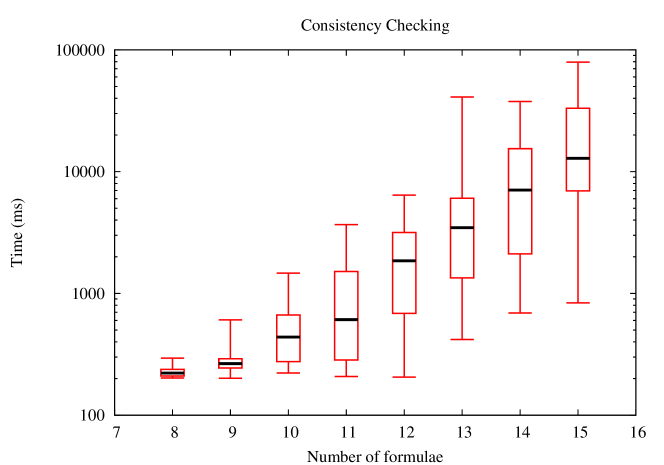
Figure 3: Log-plot summarising the time complexity of consistency checking.

Figure 4 illustrates the discrepancy between the number of combinations of formulae and the number of redundancy checks that were actually performed. The number of combinations for $n$ formulae is $n*2^{n-1}$ but the optimisation often led to much smaller number. As one can see from the experiments on 9 formulae, it is potentially necessary to check almost all the combinations but the method proposed in this paper requires on average less than 10 per cent of the checks and the relative number decreases with the number of formulae.

The actual running times, as reported in Figure 3, depend crucially on the chosen method for consistency checking: automata-based Algorithm 4 in our case. Our algorithm for enumerating all smallest inconsistent subsets is robust with respect to the consistency checking algorithm used. Hence any other consistency (or realisability) tool could be used, but that would only affect the actual running times, but not the number of checks, reported in Figure 4.

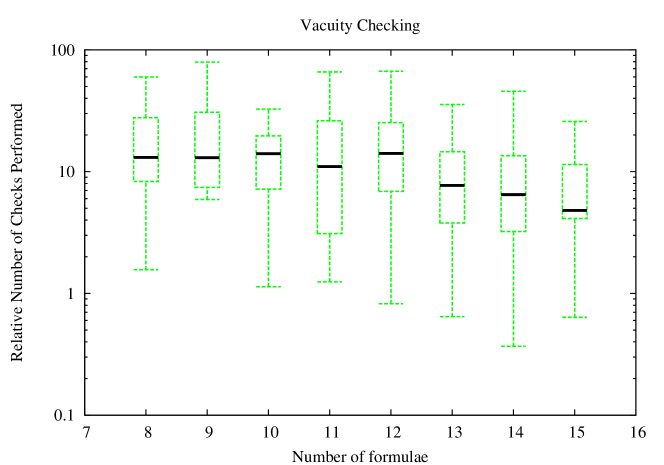
Figure 4: Log-plot with the relative number of checks for redundancy checking.

5.2 Case Study: Aeroplane Control System

In order to demonstrate the full potential of the proposed sanity checking, we apply all the steps in a sequence. First, the whole requirements document is checked for consistency and redundancy and only the consistent and non-redundant subset is then evaluated with respect to its completeness. A sensible exposition of the effectiveness of completeness evaluation proposed in this paper requires more elaborate approach than using random formulae as the input requirements document.

For that purpose a case study has been devised that demonstrates the capacity to assess coverage of requirements and to recommend suitable coverage-improving LTL formulae. The requirements document was written by a requirements engineer whose task was to evaluate to method, and we only use random formulae as candidates for coverage improvement. The candidate formulae were built based on the atomic proposition that appeared in the input requirements and only very simple generated formulae were selected. It was also required that the candidates do not form an inconsistent or tautological set. Alternatively, pattern-based [16] formulae could be used as candidates. The methodology is general enough to allow semi-random candidates generated using patterns from input formulae. For example if an implication is used as the input formula, the antecedent may not be required by the other formulae which may not be according to user’s expectations.

The case study attempts to propose a system of LTL formulae that should control the flight and more specifically the landing of an aeroplane. The LTL formulae and the atomic propositions they use are summarised in Figure 5. The requirements are divided into 3 categories similarly as in the text: $A$ requirements represent assumptions and $R$ and $F$ stand for required and forbidden behaviour, respectively. The grayed formulae were found either redundant or inconsistent and were not included in the completeness evaluation.

• The plane is on the ground only if its speed is less or equal to 200 mph.

• The plane will eventually land and every landing will result in the plane being on the ground.

• If the plane is not landing its speed is above 200 mph.

• Whenever the undercarriage is down, first the speed must be at most 100 mph and second the plane must eventually land on the ground.

• Whenever the plane is not landing its height above ground is not zero.

• At any time during the flight it holds that either the plane if flying faster than 200 mph or it eventually touches the ground.

• The landing process entails that eventually: (1) the speed will remain below 200 mph indefinitely and (2) after some finite time the speed will also remain below 100 mph.

• The landing process also entails that the plane should eventually slow down from 200 mph to 100 mph (during which the speed never goes above 200 mph).

• Whenever flying faster than 200 mph, the undercarriage must be retracted.

• At some point in the future, the plane should commence landing, then detract the undercarriage until finally the speed is below 100 mph.

• In the future the plane will be decommissioned: it will land and then either never flying faster than 100 mph or always slowing down below 200 mph.

• At some point in the future, the speed will be below 200 mph and the undercarriage retracted. Immediately before that and while the speed is still above 200 mph the undercarriage is detracted in two consecutive steps.

• The plane will eventually be on the ground after which it will never take off again.

Figure 5: The two tables explain the shorthands for atomic propositions and list the LTL requirements.

Consistency

The three categories of requirements are checked for consistency and redundancy separately. The environmental assumptions form a consistent set. The set of required behaviour contained two smallest inconsistent subsets. The requirement R4 is inconsistent with R6, hence we have choose R4 as more important and exclude R6 from the collection. The second inconsistent subset was: R1, R2, R5. There we chose to preserve R1 and R2, leaving out the possibility to decommission a plane.

Redundancy

After regaining consistency of the required behaviour, our sanity checking procedure detects no redundancy in this set. On the other hand there are two redundant environmental assumptions. The assumption A5 is implied by the conjunction of A1 and A3 and is thus redundant. It also holds that any environment in which A2 and A3 are true also satisfies A6. Hence both A5 and A6 can be removed without changing the set of sensible behaviour in the environment.

Completeness

Initially, the remaining required and forbidden behaviour together does not cover the environment assumptions at all, i.e. the coverage is 0. There simply are so many possible paths allowed by the assumptions which are not considered in the requirements, that our metric evaluated the coverage to 0. Given the way the coverage is calculated, it must be the case that for every path in the assumption automaton there was not a single path in the requirements automaton that would not violate some of the edge labels of the assumptions. There is thus a considerable space for improvement. The completeness improving process we are about to describe begins by generating a set of candidate requirements among which those with the best resulting coverage are selected. Table 1 summarises the process.

The first formula selected by the Algorithm 5 and leading to coverage of $9.1$ per cent was a simple $\varphi_{1}=\operatorname{\mathcal{G}}(\neg l)$: “The plane will never land”. Not particularly interesting per se, nonetheless emphasising the fact that without this requirement, landing was never required. The formula $\varphi_{1}$ should thus be included among the forbidden behaviour. Unlike $\varphi_{1}$, the formula generated as second, $\operatorname{\mathcal{F}}(\neg b\wedge\neg l)$ : “At some point the plane will fly faster than 200 mph and will not be in the process of landing”, should be included among the required behaviour. This formula points out that the required behaviour only specifies what should happen after landing, unlike the assumptions, which also require flight. The third and final formula was $\operatorname{\mathcal{F}}(\neg l\operatorname{\mathcal{U}}(a\vee b))$: “Eventually it will hold that the landing does not commence until either: (1) the plane is already on the ground or (2) the speed decreased below 200 mph”. This last formula connects flight and landing and its addition (among the required behaviour) entails coverage of $54.9$ per cent.

There are two conclusion one can draw from this case study with respect to the completeness part of sanity checking. First, the requirements are generated automatically, they are relevant and already formalised, thus amenable to further testing and verification. Second, the new requirements can improve the insight of the engineer into the problem. Both of these properties are valuable on their own, even though the method did not finish with 100 per cent coverage. The method produced further, coverage-improving formulae but even the best formulae only negligible improved the coverage and thus the engineer decided to stop the process.

Table 1: Iterations of the completeness evaluation algorithm for the Aeroplane Control System.

iteration	suggested formula	resulting system	coverage of $\mathcal{A}_{A}$ by $\mathcal{A}_{n}$
1	$\varphi_{1}=\operatorname{\mathcal{G}}(\neg l)$	$\mathcal{A}_{1}=\mathcal{A}_{R\vee\overline{F}\vee\overline{\varphi_{1}}}$	9.1%
2	$\varphi_{2}=\operatorname{\mathcal{F}}(\neg b\wedge\neg l)$	$\mathcal{A}_{2}=\mathcal{A}_{R\vee\overline{F}\vee\overline{\varphi_{1}}\vee\varphi_{2}}$	39.4%
3	$\varphi_{3}=\operatorname{\mathcal{F}}(\neg l\operatorname{\mathcal{U}}(a\vee b))$	$\mathcal{A}_{3}=\mathcal{A}_{R\vee\overline{F}\vee\overline{\varphi_{1}}\vee\varphi_{2}\vee\varphi_{3}}$	54.9%

5.3 Alternative LTL to Büchi Translations

Although the running time experiments were one of the priorities of the original paper [2], their purpose was to investigate the effects of the proposed optimisations and not the concrete time measurements. In other words, the subject of our investigation was the asymptotic behaviour of the algorithms and how effectively does the algorithm scale with the number of formulae in the average and in the extrema. Given our recent cooperation with Honeywell and their interest in checking sanity of real-world, industry-level sets of requirements, the actual running times became of particular interest as well.

Initial experiments revealed, however, that on larger sets of requirements and especially when more complex individual requirements were involved, the proposed sanity checking algorithms were unable to cope with the computational complexity. The bottleneck proved to be the algorithm translating LTL formulae – conjunctions of the original requirements – into Büchi automata. The translator incorporated in DiVinE is sufficiently fast on small formulae that commonly occur in software verification and was never intended to be used with larger conjunctions. Thus, to enable checking sanity of real-world sets of requirements, we have reimplemented the algorithms to employ the state-of-the-art LTL to Büchi translator SPOT [15] in a tool called Looney. As the case study summarising our cooperation with Honeywell in Section 5.4 shows, Looney is able to process much larger formulae than the original tool and also to incorporate a larger number of formulae into the sanity checking process.

The reimplementation of consistency was relatively straightforward since SPOT can be interfaced via a shared library with an arbitrary C++ application. Even though this enforced us to use the internal implementation of formulae from SPOT, which was different the one we had before, SPOT offers an adequate set of formulae-manipulating operations that allowed the translation of our algorithms, without their needing to be considerably modified. The reimplementation of the coverage algorithms was complicated by the fact that the product of SPOT is a transition-based Büchi automaton, whereas the algorithm of Section 4 expects state-based automata: the difference is that transitions rather than states are denoted as accepting.

This shift requires modification of the coverage evaluation, more precisely the definition of $\Lambda(\mathcal{A}_{1},\mathcal{A}_{2})$ of the coverage among automata. Before, the number $m$ in the denominator referred to the number of almost-simple paths of $\mathcal{A}_{1}$ that ended in an accepting vertex (state). We propose to redefine $m$ as the number of almost-simple paths that end in an accepting edge (transition). It is clear that the coverage reported by the original and the new metrics would differ: first, because the automata are generated using different methods and may thus be structurally different and, second, because the redefined metric considers different sets of almost-simple paths. With the alternative definition of $m$ one can easily incorporate translators that produce transition-based automata (though parsing these automata may still require some degree of modification due to incompatibility of internal structures representing the automata).

Therefore, in order to reestablish admissibility of the new evaluation as an adequate coverage metric, we have repeated the experiment with the aeroplane control system. As was to be expected given the above argumentation, the concrete evaluation of individual formulae differed from our original experiments. Specifically, the formula first generated ($\operatorname{\mathcal{G}}(\neg l)$) was evaluated with coverage 12.9 per cent (instead of 9.1); the second formula $\operatorname{\mathcal{F}}(\neg b\wedge\neg l)$ with 35.0 (instead of 39.4); and the third formula $\operatorname{\mathcal{F}}(\neg l\operatorname{\mathcal{U}}(a\vee b))$ with 61.1 (instead of 54.9). Hence there are two observation to be made. First, even though the coverage numbers differ for individual formulae, the same triple was produced by the modified algorithm. Moreover, the three formulae were produced in the same order, thus the new metric behaves appropriately even when a new set of requirements is obtained as a disjunction of the old set with the generated coverage-improving formula.

5.4 Industrial Evaluation

As a further extension to the original paper [2], we have evaluated our consistency and redundancy checking method on a real-life sets of requirements obtained in cooperation with Honeywell International. We did not extend this part of evaluation to the completeness checking since that would require writing a new set of requirements with separating the assumptions. The case study consisted of four Simulink models; each has been associated with a set of formalised requirements in the form of LTL formulae. The precise requirements are unfortunately confidential, but we provide statistics regarding the complexity of the requirement documents. The formalisation of the requirements that were originally given in natural language form has been done with the help of the ForReq tool. The tool allows the user to write formal requirements with the help of the specification patterns [16] and some of their extensions. See [3] for a detailed description of the tool.

Out of the four models, one (Lift) was a toy model used in Honeywell to evaluate the capabilities of ForReq, three (VoterCore, AGS, pbit) were models of real-world avionics subsystems. As the focus of this paper is model-less sanity checking, we ignored the models themselves and only considered the formalised requirements. The results of our experiments are summarised in Table 2.

The table reports that the largest collection of requirements consisted of 10 formulae, which can hardly be considered as a demonstration of scaling to industrial level. Even though some of the requirements were extremely complicated (with as many as 100 LTL operators), there is clearly a large space for improvement. It would certainly be possible to use a different algorithm for performing a single consistency check, but the number of these checks that needs to be performed is an independent issue left for future work. In all four cases, the whole set of requirements was consistent. As for redundancy, we have identified two cases where a formula was implied by another one. This is shown in the redundancy result column. The number displayed in the mem(MB) column represent the maximal (peak) amount of memory used.

The experiments, with the exception of the last one, were run on a dedicated Linux workstation with Intel Xeon E5420 @ 2.5 GHz and 8 GB RAM. The last experiment (pbit) was run on a Linux server with Intel X7560 @ 2.27 GHz and 450 GB RAM. The last experiment was a consistency check only as the redundancy checking took too much time. The reason for such great consumption of time (and memory) is that the formulae in the pbit set of requirements are rather complex, some of them even using precise specification of time. For more details about the time extension of LTL and its translation to standard LTL, see [3].

Table 2: Results of consistency and redundancy checking on an industrial case study.

model	no. of	consistency			redundancy
name	formulae	result	time(s)	mem(MB)	result	time(s)	mem(MB)
VoterCore	3	OK	0.1	21.6	OK	0.4	22.4
AGS	5	OK	0.1	23.5	$\varphi_{4}\Rightarrow\varphi_{2}$	0.7	23.6
Lift	10	OK	73.6	58.5	$\varphi_{1}\Rightarrow\varphi_{5}$	9460.5	1474.5
pbit	10	OK	210879.0	22 649.0	—	—	—

6 Conclusion

This paper further expands the incorporation of formal methods into software development. Aiming specifically at the requirements stage we propose a novel approach to sanity checking of requirements formalised in LTL formulae. Our approach is comprehensive in scope integrating consistency, redundancy and completeness checking to allow the user (or a requirements engineer) to produce a high quality set of requirements easier. The expert knowledge of LTL is not a prerequisite for using the method, given the existence of automated translator from English. On the other hand, there are certain limitations with respect to the number of requirements checked concurrently, and larger collections may require manually dividing into smaller sets.

Especially in the earliest stages of the requirements elicitation, when the engineers have to work with highly incomplete, and often contradictory sets of requirements, could our sanity checking framework be of great use. Other realisability checking tools can also (and with better running times) be used on the nearly final set of requirements but our process uniquely target these crucial early states. First, finding all inconsistent subsets instead of merely one helps to more accurately pinpoint the source of inconsistency, which may not have been elicited yet. Second, once working with a consistent set, the requirements engineer gets further feedback from the redundancy analysis, with every minimal redundancy witness pointing to a potential lack of understanding of the system being designed. Finally, the semi-interactive coverage-improving generation of new requirements attempts to partly automate the process of making the set of requirements as detailed as to prevent later development stages from misinterpreting a less thoroughly covered aspect of the system. We demonstrate this potential application on case studies of avionics systems.

The above described addition to the standard elicitation process may seem intrusive, but the feedback we have gather from requirements engineers at Honeywell were mostly positive. Especially given the tool support for each individual steps of the process – pattern-based automatic translation from natural language requirements to LTL and the subsequent fully- and semi-automated techniques for sanity checking – a fast adoption of the techniques was observed. Many of the engineers reported a non-trivial initial investment to assume the basics of LTL, but in most cases the resulting overall savings in effort outweighed the initial adoption effort. After the first week, the overhead of tool-supported formalisation into LTL was less than 5 minutes per requirement, while the average time needed for corresponding stages of requirements elicitation decreased by 18 per cent.

We have also accumulated a considerable amount of experience from employing the sanity checking on real-world sets of requirements during our cooperation with Honeywell International. Of particular importance was the realisation that the time requirements of our original implementation effectively prevented the use of sanity checking on industrial scale. In order to ameliorate the poor timing results we have reimplemented the sanity checking algorithms using the state-of-the-art LTL to Büchi translator SPOT, which accelerated the process by several orders on magnitude on larger sets of formulae. Another important observation was that the concept of model-based vacuity is desirable to be translated into the model-free environment more directly than as redundancy. We thus extend the sanity checking process with the capacity to generate vacuity witnesses (using the formally described theory of path-quantified formulae). Finally, we summarise these and other observations in a case consisting of four sets of requirements gathered during the development of industry-scale systems.

One direction of future research is the pattern-based candidate selection mentioned above. Even though the selected candidates were relatively sensible in presented experiments, using random formulae can produce useless results. Finally, experimental evaluation on real-life requirements and subsequent incorporation into a toolchain facilitating model-based development are the long term goals of the presented research. This paper also lacks formal definition of total coverage (which the proposed partial coverage merely approximates). We intend to formulate an appropriate definition using uniform probability distribution: which would also allow to compute total coverage without approximation and would not be biased by concrete LTL to BA translation. That solution, however, is not very practical since the underlying automata translation is doubly exponential.

References

- [1] M. Abadi, L. Lamport, and P. Wolper. Realizable and Unrealizable Specifications of Reactive Systems. In Proc. of ICALP, pages 1–17, 1989.
- [2] J. Barnat, P. Bauch, and L. Brim. Checking Sanity of Software Requirements. In Proc. of SEFM, pages 48–52, 2012.
- [3] J. Barnat, J. Beran, L. Brim, T. Kratochvíla, and P. Ročkai. Tool Chain to Support Automated Formal Verification of Avionics Simulink Designs. In Proc. of FMICS, pages 78–92, 2012.
- [4] J. Barnat, L. Brim, M. Češka, and P. Ročkai. DiVinE: Parallel Distributed Model Checker. In Proc. of HiBi/PDMC, pages 4–7, 2010.
- [5] I. Beer, S. Ben-David, C. Eisner, and Y. Rodeh. Efficient Detection of Vacuity in Temporal Model Checking. Form. Methods Syst. Des., 18(2):141–163, 2001.
- [6] R. Bloem, A. Cimatti, K. Greimel, G. Hofferek, R. Könighofer, M. Roveri, V. Schuppan, and R. Seeber. RATSY – A New Requirements Analysis Tool with Synthesis. In Proc. of CAV, pages 425–429, 2010.
- [7] S. Blom, W. Fokkink, J. Groote, I. van Langevelde, B. Lisser, and J. van de Pol. CRL: A Toolset for Analysing Algebraic Specifications. In CAV, volume 2102 of LNCS, pages 250–254. Springer, 2001.
- [8] J. Bormann and H. Busch. Method for the Determination of the Quality of a Set of Properties, Usable for the Verification and Specification of Circuits. U. S. Patent No. 7,571,398 B2, 2009.
- [9] W. Chan, R. J. Anderson, P. Bea, S. Burns, F. Modugno, D. Notkin, and J. D. Reese. Model Checking Large Software Specifications. IEEE T. Software Eng., 24:498–520, 1998.
- [10] H. Chockler, O. Kupferman, R. Kurshan, and M. Y. Vardi. A Practical Approach to Coverage in Model Checking. In CAV, volume 2102 of LNCS, pages 66–78. Springer, 2001.
- [11] H. Chockler, O. Kupferman, and M. Y. Vardi. Coverage Metrics for Temporal Logic Model Checking. In TACAS, volume 2031 of LNCS, pages 528–542. Springer, 2001.
- [12] A. Cimatti, E. M. Clarke, E. Giunchiglia, F. Giunchiglia, M. Pistore, M. Roveri, R. Sebastiani, and A. Tacchella. NuSMV 2: An OpenSource Tool for Symbolic Model Checking. In CAV, volume 2404 of LNCS, pages 241–268. Springer, 2002.
- [13] A. Cimatti, M. Roveri, V. Schuppan, and A. Tchaltsev. Diagnostic Information for Realizability. In Proc. of VMCAI, pages 52–67, 2008.
- [14] C. Courcoubetis, M. Y. Vardi, P. Wolper, and M. Yannakakis. Memory-Efficient Algorithms for the Verification of Temporal Properties. Form. Method Syst. Des., 1:275–288, 1992.
- [15] A. Duret-Lutz. LTL Translation Improvements in Spot. In Proc. of VECoS, pages 72–83, 2011.
- [16] M. B. Dwyer, G. S. Avrunin, and J. C. Corbett. Property Specification Patterns for Finite-State Verification. In Proc. of FMSP, pages 7–15, 1998.
- [17] G. Feierbach and V. Gupta. True Coverage: A Goal of Verification. In Proc. of ISQED, pages 75–78, 2003.
- [18] M. P. E. Heimdahl and N. G. Leveson. Completeness and Consistency Analysis of State-Based Requirements. In Proc. of ICSE, pages 3–14, 1995.
- [19] M. Hinchey, M. Jackson, P. Cousot, B. Cook, J. P. Bowen, and T. Margaria. Software Engineering and Formal Methods. Commun. ACM, 51:54–59, 2008.
- [20] S. Katz, O. Grumberg, and D. Geist. ”Have I Written Enough Properties?” - A Method of Comparison Between Specification and Implementation. In Proc. of CHARME, pages 280–297, 1999.
- [21] R. Konighofer, G. Hofferek, and R. Bloem. Debugging Formal Specifications Using Simple Counterstrategies. In Proc. of FMCAD, pages 152–159, 2009.
- [22] O. Kupferman. Sanity Checks in Formal Verification. In CONCUR, volume 4137 of LNCS, pages 37–51. Springer, 2006.
- [23] O. Kupferman and M. Y. Vardi. Vacuity Detection in Temporal Model Checking. STTT, 4:224–233, 2003.
- [24] N. Leveson. Completeness in Formal Specification Language Design for Process-Control Systems. In Proc. of FMSP, pages 75–87, 2000.
- [25] M. Liffiton and K. Sakallah. Algorithms for Computing Minimal Unsatisfiable Subsets of Constraints. J. Autom. Reasoning, 40(1):1–33, 2008.
- [26] I. Lynce and J. P. Marques-Silva. On Computing Minimum Unsatisfiable Cores. In Proc. of SAT, pages 305–310, 2004.
- [27] S. P. Miller, A. C. Tribble, and M. P. E. Heimdahl. Proving the Shalls. In FME, volume 2805 of LNCS, pages 75–93. Springer, 2003.
- [28] A. Rajan, M. W. Whalen, and M. P. E. Heimdahl. Model Validation using Automatically Generated Requirements-Based Tests. In Proc. of HASE, pages 95–104, 2007.
- [29] S. Regimbal, J.-F. Lemire, Y. Savaria, G. Bois, E. Aboulhamid, and A. Baron. Automating Functional Coverage Analysis Based on an Executable Specification. In Proc. of IWSOC, pages 228–234, 2003.
- [30] S. Roy, S. Das, P. Basu, P. Dasgupta, and P. P. Chakrabarti. SAT Based Solutions for Consistency Problems in Formal Property Specifications for Open Systems. In Proc. of ICCAD, pages 885–888, 2005.
- [31] K. Rozier and M. Y. Vardi. LTL Satisfiability Checking. In SPIN, volume 4595 of LNCS, pages 149–167. Springer, 2007.
- [32] V. Schuppan. Towards a Notion of Unsatisfiable and Unrealizable Cores for LTL. Sci. Comput. Program., 77(7-8):908–939, 2012.
- [33] S. Tasiran and K. Keutzer. Coverage Metrics for Functional Validation of Hardware Designs. IEEE Des. Test. Comput., 18(4):36–45, 2001.
- [34] M. W. Whalen, A. Rajan, M. P. E. Heimdahl, and S. P. Miller. Coverage Metrics for Requirements-Based Testing. In Proc. of ISSTA, pages 25–36, 2006.