Spinor-vector duality and light Z’ in heterotic strings

Abstract:

We discuss the construction of heterotic–string models that allow for the existence of an extra $Z^{\prime}$ at low scales. One of the main difficulties encountered is that the desired symmetries tend to be anomalous in the prevailing three generation constructions. The reason is that these models utilise the symmetry breaking pattern $E_{6}\rightarrow SO(10)\times U(1)_{\zeta}$ by GGSO projections. Consequently, $U(1)_{\zeta}$ becomes anomalous. The spinor–vector duality that was observed in the fermionic $Z_{2}\times Z_{2}$ orbifold compactifications is used to construct a phenomenological three generation Pati–Salam heterotic–string model in which $U(1)_{\zeta}$ is anomaly free and therefore can be a component of a low scale $Z^{\prime}$. The model implies existence of matter states at the $Z^{\prime}$ breaking scale, which are required for anomaly cancelation. Moreover, the string model gives rise to exotic states, which are $SO(10)$ singlets but carry exotic $U(1)_{\zeta}$ charges. These states arise due to the breaking of $E_{6}$ by discrete Wilson lines and provide natural dark matter candidates. Initial indications suggest that the existence of additional gauge symmetries at the TeV scale may be confirmed in run II of the LHC experiment.

1 Introduction

The Standard Model of elementary particle physics continues to provide an accurate parameterisation of all particle physics observations. The data from the lepton colliders during the 1990s confirmed the non–Abelian nature of the electroweak and strong interactions to an unprecedented precision. The observation of a Higgs–like state at the LHC represents another triumph of the model. The task of future experiments will be to continue to probe the Standard Model parameterisation to better and better precision, and possibly discover its plausible extensions. It is also not implausible that the Standard Model is all there is at the energy scales within reach of the LHC and possibly within reach of collider experiments in the decades to come. This does not diminish from the vitality of these experiments and their importance. If nature consists solely of the Standard Model in this energy range we ought to confirm that this is the indeed the case in future experiments. The challenge to develop the instruments that can probe nature at the increasing energy scales benefits the societies that pursue this endeavour and ultimately offers them technological and economic supremacy. At the present state of affairs the standard model consists of three gauge sectors, three generations of matter families with six chiral multiplets per family, and a single electroweak scalar doublet. Perhaps the most striking feature of the Standard Model is the fact that its matter content fits into chiral 16 representations of $SO(10)$. The significance of this coincidence is exemplified most clearly if we consider that the Standard Model gauge quantum numbers are experimental observables. The Standard Model requires fifty–four parameters to account for these charges, whereas its embedding in $SO(10)$ reduces this number to one parameter, being the number of $SO(10)$ chiral 16 representations required to embed the Standard Model states. The success of the Standard Model provide strong support for the realisation of the $SO(10)$ unification structures in nature. The scale where these unification structures become relevant is, however, far removed from the electroweak scale. Evidence to this effect stem from the observed logarithmic running of the Standard Model parameters; the proton longevity; and the suppression of left–handed neutrino masses.

Despite its enormous success, the Standard Model leaves several gaps. While QCD provides an accurate parameterisation of the strong interactions in the perturbative regime, a detailed understanding of its nonperturbative infrared limit and confinement is still lacking. The gravitational effects are not accounted for. Moreover, there is a fundamental dichotomy between point quantum field theories, the calculational framework underlying the Standard Model, and general relativity, which underlie the gravitational interactions. String theories produce a self–consistent approach to the synthesis of general relativity and quantum mechanics. Furthermore, the string consistency conditions mandate the existence of gauge and matter states, similar to those that are present in the Standard Model. String theories therefore facilitate the development of a viable phenomenological approach to probe how the gravitational and gauge interactions may be reconciled.

Heterotic string theory is particularly appealing because it gives rise to spinorial representations in its perturbative spectrum, and thus enables the embedding of the Standard Model matter states in spinorial $SO(10)$ representations. The free fermionic formulation [1] of the heterotic string provides a particularly fertile framework for the construction of phenomenological string vacua with $SO(10)$ embedding of the Standard Model chiral states. It is important to note that the $SO(10)$ symmetry is broken to one of its subgroups directly at the string scale. This gives rise to the string doublet–triplet splitting mechanism. It enables the Higgs states to exist in incomplete $SO(10)$ multiplets, which facilitates the compatibility with the gauge coupling data at the electroweak scale, as well as with proton lifetime limits. The primary guides in the search of quasi–realistic string vacua are the existence of three chiral generations and their $SO(10)$ embedding.

2 Free fermionic models

A class of phenomenological string vacua that meet these criteria are the quasi–realistic string models in the free fermionic formulation. Since the early 1990s this class of models provided a laboratory to study how the phenomenological features of the Standard Model may arise from string theory. A few of the highlights include:

• Minimal Superstring Standard Model [2, 3]. Construction of string models leading to solely the MSSM spectrum below the string scale.

• Top quark mass $\rightarrow 175-180$GeV [4]. Calculation of the top and bottom quarks Yukawa couplings at the string scale yielding a prediction of the top quark mass at the electroweak scale.

• Fermion masses and CKM mixing [5].

• Stringy seesaw mechanism and neutrino masses [6].

• Gauge coupling unification [7].

• Proton stability [8]

• Squark degeneracy [9].

• Moduli fixing [10].

• Classification & Exophobia [11, 12, 13].

• Spinor–vector duality [14, 15].

It should be stressed that this free fermionic construction probes one class heterotic–string vacua, which are related to $Z_{2}\times Z_{2}$ orbifold compactification. Other classes of string vacua can be probed by using a variety of tools that have been developed over the years. These include geometrical, orbifolds, interacting world–sheet conformal field theory constructions; orientifolds. A comprehensive review of different approaches to string phenomenology is given in ref. [16].

3 $Z^{\prime}$s in free fermionic models

One of the well motivated extensions of the Standard Model is the existence of an extra gauge symmetry beyond the Standard Model. The first argument in favour of such extensions is that gauge symmetries actually exist in nature, and the assumption that an additional gauge symmetry exists is not outrageous. More concretely, we have argued that the Standard Model gauge charges strongly hint to the $SO(10)$ embedding of the Standard Model matter states. This necessitates that the Standard Model gauge symmetry is extended by at least one $U(1)$ factor. The promotion of the global baryon and lepton symmetries to a local symmetry further hints that the Standard Model gauge symmetry should be extended. This again fits well with the $SO(10)$ paradigm in which the baryon minus lepton number is gauged. Anomaly cancellation in perturbative string theory, which incorporates the Standard Model building blocks and gravity in one embrace, mandates the existence of additional gauge symmetries. Furthermore, the heterotic–string fuses those ingredients and reproduces the $SO(10)$ structure underlying the Standard Model. It should be emphasised again that the $SO(10)$ symmetry is not manifested as a gauge symmetry in the effective field theory limit of the string vacua, but merely serves as an organisional framework from that point of view. It’s ultimate role, once the full string dynamics is better understood is a story for the future. Possibly for future generations.

The Standard Model points to the existence of additional gauge symmetries, while string theory mandates their existence. Alas, the additional gauge symmetries may be broken at a high scale compared to the electroweak scale and would not be observed in contemporary collider experiments. Non–Abelian extensions of the Standard Model like $SU(5)$ is consistent with proton decay limits only if the $SU(5)$ symmetry is broken above $10^{16}GeV$. The most plausible extension of the Standard Model within reach of contemporary collider experiments is an Abelian gauge symmetry.

The heterotic–string models in the free fermionic formulation reproduce the general features of the Standard Model and provide a setting to investigate additional gauge symmetries in quasi–realistic string constructions. While additional spacetime vector bosons are abundant in the string models, the possibility that they remain massless to low energy scales is far less obvious. In fact for a variety of reasons most of the additional gauge symmetries have to be broken at a scale beyond the reach of the LHC. Exploration of additional $Z^{\prime}$s in free fermionic models started in the early nineties. The first case to be considered [17] was the combination

$$U(1)_{Z^{\prime}}={3\over 2}U(1)_{B-L}-2U(1)_{R}\in SO(10).$$ (1)

Existence of this $Z^{\prime}$ at the TeV scale ensures the suppression of proton decay from dimension four operators, which are endemic in supersymmetric extensions of the Standard Model. However, the underlying $SO(10)$ symmetry in the string models dictates that the Dirac mass term of the tau neutrino is equal that of the top quark. Breaking the $U(1)_{Z^{\prime}}$ symmetry of eq. (1) at the TeV scale generates a low scale seesaw, which implies either a relatively heavy tau neutrino or that some scalar fields get an ad hoc VEV of order $O(1keV)$ [6]. A more natural possibility is that this $U(1)_{Z^{\prime}}$ symmetry is broken at a high scale, which generates a large scale seesaw and naturally produces light neutrino masses [6]. However, high scale breaking of the $U(1)_{Z^{\prime}}$ symmetry of eq. (1) would naively generate effective dimension four proton decay mediating operators via the nonrenormalisable terms

$$QLd{\cal N}\phi^{n}~{}~{}~{}~{}~{}~{}~{}~{}~{}~{}~{}~{}~{}~{}~{}~{}udd{\cal N}\phi^{n}$$ (2)

where ${\cal N}$ and $\bar{\cal N}$ are the components of the Higgs fields that break $U(1)_{Z^{\prime}}$, and $\phi^{n}$ is a string of states that get VEVs of the order of the string scale. The induced dimension four operators are proportional to the $U(1)_{Z^{\prime}}$ symmetry breaking scale, and in the absence of additional suppression generate proton decay at an unacceptable rate. It is noted that in heterotic string models the problems of proton stability and light neutrino masses are in conflict. Namely, the first prefers a low $U(1)_{Z^{\prime}}$ breaking scale, whereas the second works better with a high $U(1)_{Z^{\prime}}$ breaking scale. Another possibility is the existence of alternative gauge symmetries in the string vacua, which suppress the proton decay mediating operators but allow a high breaking of $U(1)_{Z^{\prime}}$ and therefore a high seesaw mass scale. Such gauge symmetries within reach of the LHC should additionally: 1. be anomaly free; 2. be family universal; 3. allow for quark and lepton mass terms. Pati proposed in ref. [18] that the family universal anomaly free combination of the flavour $U(1)$s in the model of ref. [19] plays a role in adequately suppressing proton decay mediating operators, as well as allowing for suppression of left–handed neutrino masses via the seesaw mechanism. In ref. [20] it was shown that the $U(1)$ symmetry discussed in ref. [18] must be broken near the string scale. Other $U(1)$ symmetries that may play a role in suppressing proton decay mediating operators while allowing for a high seesaw mass scale were discussed in refs. [21]. To understand the properties of these extra $U(1)$ symmetries, and why they fail to materialise as low scale $Z^{\prime}$s, it is instrumental to first consider the general structure of the free fermionic models.

4 Free fermionic constructions

In the free fermionic construction all the degrees of freedom needed to cancel the world–sheet conformal anomaly are represented in terms of Majorana–Weyl free fermions. It is important to emphasise that the fermions are free only at a specific point in the moduli space and moving away from that point entails adding world–sheet Thirring interactions [22], which preserve the conformal symmetry. The constructions are mathematically equivalent to bosonic compactifications on six dimensional tori, with the world–sheet Thirring interactions being equivalent to the exact marginal deformations in the bosonic models. In four dimensional models in the light–cone gauge the total number of world–sheet fermions is twenty left–moving and forty–four right–moving real two dimensional fermions. Eight of the left–moving fermions correspond to the Ramond–Neveu–Schwarz fermions in the supersymmetric side of the ten dimensional heterotic–string, whereas the additional twelve correspond to the six left–moving compactified coordinates. Similarly, on the right–moving side twelve real fermions correspond to the six compactified dimensions. The remaining thirty–two fermions are combined into sixteen complex fermions that give rise to the rank sixteen gauge symmetry of the heterotic–string in ten dimensions. The sixty–four world–sheet fermions are typically denoted by $\{\psi^{1,2},(\chi,y,\omega)^{1,\cdots,6}|({\bar{y}},{\bar{\omega}})^{1,\cdots,6},{\bar{\psi}}^{1,\cdots,5},{\bar{\eta}}^{1,2,3},{\bar{\phi}}^{1,\cdots,8}\}$, where ${\bar{\psi}}^{1,\cdots,5}$ are the Cartan generators of the $SO(10)$ GUT group.

Under parallel transport around the non–contractible loops of the torus representing the vacuum to vacuum amplitude, the world–sheet fermions pick up a phase. These transformation properties are summarised in sixty–four dimensional vectors. Invariance of the vacuum to vacuum amplitude under modular transformations leads to a set of constraints on the phase assignments. Summation over all the possible assignments with appropriate phases to render a sum which is modular invariant produces the partition function. Models in the free fermionic construction are therefore obtained by specifying a set of boundary condition basis vectors and the one–loop summation phases in the partition function. The resulting string vacuum may be equivalently specified as an orbifold of a six dimensional internal torus, and corresponds to compactification on some Calabi-Yau manifold in the smooth effective field theory limit. The moduli deformations of the six dimensional internal manifold are represented in the fermionic construction in terms of world–sheet Thirring interactions. The massless spectrum and interactions are obtained in the free fermionic formalism by applying the Generalised GSO projections and can be extracted in relative ease.

The early free fermionic heterotic–string models were constructed by specifying a set of eight (or nine) basis vectors. The first five basis vectors consist of the so–called NAHE–set [23], and are common in all the early phenomenological models. The gauge group at the level of the NAHE–set is $SO(10)\times SO(6)^{3}\times E_{8}$, with forty–eight multiplets in the spinorial $16$ representation of $SO(10)$. The $SO(10)$ symmetry is broken to one of its subgroups and the numbers of generations is reduced to three by adding three or four basis vectors to the NAHE–set. The phenomenological properties of the models are then extracted by calculating trilevel and higher order terms in the superpotential and by analysing its flat directions.

5 Toward string predictions

The phenomenological three generation models may also lead to signatures beyond the Standard Model, that may be tested in future experiments. It is important to note that the actual correlation of these effects with experimental data will necessarily employ an effective field theory parameterisation. Among the possibilities we may list: specific patterns of supersymmetry breaking, which may be seen in forthcoming collider experiments; additional spacetime gauge bosons that similarly lead to specific collider signatures; and the existence of exotic matter that produces a variety of dark matter candidates. Recently the ATLAS and CMS experiments at the LHC reported possible excesses that are compatible with the existence of additional vector bosons of order 2TeV [24]. A comprehensive analysis of possible extra vector bosons in string models was undertaken in ref. [25].

However, the construction of string models that allow the existence of an extra $Z^{\prime}$, of the type that may be observed by the LHC experiments at the TeV scale, is highly non–trivial. To see why this is the case we have to examine the patterns of $SO(10)$ symmetry breaking induced by the basis vectors beyond the NAHE–set. The $SO(10)$ symmetry is broken to the following subgroups by the assignment of boundary conditions $b({\bar{\psi}}^{1\cdots 5}_{1\over 2})$:

$$1.~{}b\{{{\bar{\psi}}_{1\over 2}^{1\cdots 5}{~{}{\bar{\eta}}^{1}}~{}{{\bar{\eta}}^{2}}~{}{{\bar{\eta}}^{3}}}\} = \{{1\over 2}{1\over 2}{1\over 2}{1\over 2}{1\over 2}{{1\over 2}}{{1\over 2}}{{1\over 2}}\}\Rightarrow~{}SU(5)\times U(1)~{}\times U(1)\times U(1)\times U(1)$$ (3)

$$2.~{}b\{{{\bar{\psi}}_{1\over 2}^{1\cdots 5}{~{}{\bar{\eta}}^{1}}~{}{{\bar{\eta}}^{2}}~{}{{\bar{\eta}}^{3}}}\} = \{~{}1~{}1~{}1~{}0~{}0~{}{0}{0}{0}~{}\}\Rightarrow SO(6)\times SO(4)\times U(1)\times U(1)\times U(1).$$ (4)

The breaking $SO(10)~{}~{}\rightarrow SU(3)_{C}\times SU(2)_{L}\times U(1)_{C}\times U(1)_{L}$ is obtained by combining (3) and (4) in two separate basis vectors. The Left–Right Symmetric (LRS) breaking pattern $SO(10)\rightarrow SU(3)_{C}\times SU(2)_{L}\times SU(2)_{R}\times U(1)_{B-L}$ may be obtained by including two $SO(10)$ breaking basis vectors with the first inducing the Pati–Salam breaking pattern in eq. (4) and the second

$$3.~{}b\{{{\bar{\psi}}_{1\over 2}^{1\cdots 5}~{}{{\bar{\eta}}^{1}}~{}{{\bar{\eta}}^{2}}~{}{{\bar{\eta}}^{3}}}\} = \{{1\over 2}{1\over 2}{1\over 2}~{}0~{}0~{}{{1\over 2}}{{1\over 2}}{{1\over 2}}\}\Rightarrow$$

$$~{}~{}~{}~{}~{}~{}~{}~{}~{}~{}~{}~{}~{}~{}~{}~{}~{}~{}SU(3)_{C}\times U(1)_{C}\times SU(2)_{L}\times SU(2)_{R}\times{U(1)}\times{U(1)}\times{U(1)}$$

A key difference between the $SU(5)\times U(1)$, $SO(6)\times SO(4)$ and $SU(3)\times SU(2)\times U(1)^{2}$ cases, which are obtained by using the boundary condition assignments in eqs. (3) and (4), versus the LRS models is with respect to the charges of the Standard Model family states under the three $U(1)$ symmetries, $U(1)_{1,2,3}$, corresponding to the world–sheet complex fermions ${\bar{\eta}}^{1,2,3}$. In the first class of models $Q_{U(1)_{j}}(16=\{Q,L,U,D,E,N\})~{}=~{}+{1\over 2}$, i.e. all the states in the $16$ $SO(10)$ spinorial representation in a given twisted plane have common charge $\pm 1/2$. Therefore, in these models $U(1)_{1,2,3}$, as well as the the family universal combination $U(1)_{\zeta}=U(1)_{1}+U(1)_{2}+U(1)_{3}$, are anomalous. In the LRS models on the other hand, the charges differ between the left– and right–handed states, with

$$Q_{U(1)_{j}}(~{}~{}~{}~{}~{}~{}~{}~{}~{}~{}~{}~{}~{}~{}~{}Q_{L}~{}~{}~{},~{}~{}~{}L_{L}~{}~{}~{}~{}~{}~{}~{}~{}~{}~{}~{}~{}~{}~{}~{})~{}~{}~{}=~{}-{1\over 2}~{},$$ (6)

$$Q_{U(1)_{j}}(~{}Q_{R}=\{U,D\}~{}~{},~{}~{}L_{R}=\{E,N\}~{})~{}=~{}+{1\over 2}~{}.$$ (7)

Consequently, in these models the $U(1)_{1,2,3}$ symmetries as well as the family universal combination $U(1)_{\zeta}$ are anomaly free. Three generation left–right symmetric string derived models were presented in ref. [26]. Some of the models presented contain untwisted Higgs bi–doublets that can be used to generate quasi–realistic fermion mass spectrum from renormalisable and non–renormalisable superpotential terms.

For a $U(1)$ symmetry to remain unbroken down to low scales it must be anomaly free. To be viable at scales within reach of the LHC it must also be family universal. The family universal combination $U(1)_{\zeta}$ satisfies the two requirements. To study its signatures at low scales we build a string inspired model [27] with the charge assignments in eqs. (6, 7). Considering only the Standard Model matter states leads to a mixed $SU(2)_{L}^{2}\times U(1)_{\zeta}$ anomaly. The string derived models are anomaly free and contain extra states that cancel the anomaly. To construct a model free of all anomalies $SU(2)_{L/R}$ doublets are added to the model. To facilitate gauge coupling unification we may also add colour triplets. We impose that the charge assignments in the string inspired model are compatible with the charges in the string derived models. Extrapolating the gauge coupling from the GUT unification scale to the electroweak scale and imposing the experimental values $\alpha_{S}(M_{Z})\approx 0.1$ and $\sin^{2}\theta(M_{Z})\approx 0.231$ yields the following hierarchy of scales [27]

$$M_{SUSY}\approx 1{\rm TeV};~{}~{}M_{Z^{\prime}}>10^{8}{\rm GeV};~{}~{}M_{D}>10^{12}{\rm GeV};~{}~{}M_{R}\approx M_{string},$$

where $M_{R}$ is the symmetry breaking scale of $SU(2)_{R}$, which induces the seesaw mechanism and the suppression of left–handed neutrino masses. It is noted that compatibility of string gauge coupling unification with the gauge coupling parameters at the electroweak scale requires that $M_{Z^{\prime}}$ is heavier than $10^{8}$GeV. Hence, a $Z^{\prime}$ at the TeV scale in this string inspired model is incompatible with the gauge coupling data. The root of the discrepancy can be seen to arise from the fact that the $Z^{\prime}$ charges do not admit the $E_{6}$ embedding in this model. The contrast between this model versus models that admit the $E_{6}$ embedding can be seen by examining the contributions of the intermediate gauge and matter thresholds to $\sin^{2}\theta_{W}(M_{Z})$ and $\alpha_{3}(M_{Z})$. In the case of the charge assignments in the LRS string inspired model the threshold corrections from intermediate gauge and matter scales are given by

$$\delta\left(\sin^{2}\theta_{W}(M_{Z})\right)_{\mbox{\tiny{I.T.}}} = \frac{1}{2\pi}\frac{k_{1}\alpha}{1+k_{1}}\left(\frac{12}{5}\log\frac{M_{S}}{M_{R}}-\frac{24}{5}\log\frac{M_{S}}{M_{Z^{\prime}}}-\frac{2n_{D}}{5}\log\frac{M_{S}}{M_{D}}\right),$$

$$\delta\left(\alpha_{3}(M_{Z})\right)_{\mbox{\tiny{I.T.}}} = \frac{1}{2\pi}\left(\frac{3}{2}\log\frac{M_{S}}{M_{R}}-9\log\frac{M_{S}}{M_{Z^{\prime}}}+\frac{3n_{D}}{4}\log\frac{M_{S}}{M_{D}}\right),$$ (8)

whereas in the case of models that admit the $E_{6}$ embedding the threshold corrections are given by

$$\delta\left(\sin^{2}\theta_{W}(M_{Z})\right)_{\mbox{\tiny{I.T.}}} = \frac{1}{2\pi}\frac{k_{1}\alpha}{1+k_{1}}\left(\frac{12}{5}\log\frac{M_{S}}{M_{R}}+\frac{6}{5}\log\frac{M_{S}}{M_{H}}-\frac{6}{5}\log\frac{M_{S}}{M_{D}}\right),$$

$$\delta\left(\alpha_{3}(M_{Z})\right)_{\mbox{\tiny{I.T.}}} = \frac{1}{2\pi}\left(\frac{3}{2}\log\frac{M_{S}}{M_{R}}-\frac{9}{4}\log\frac{M_{S}}{M_{H}}+\frac{9}{4}\log\frac{M_{S}}{M_{D}}\right).$$ (9)

Eqs. (8) and (9) demonstrate the cancellation between thresholds corrections of the doublets and triplets in the models that admit the $E_{6}$ embedding, which is not the case in the string inspired LRS models, as seen from eq. (8). Compatibility of heterotic–string gauge coupling unification with the gauge coupling data at the electroweak scale therefore favours string models that admit the $E_{6}$ embedding of the $U(1)_{\zeta}$ charges. As discussed above in many of the string derived models, including the flipped $SU(5)$ [28], the Pati–Salam [29] and the standard–like models [19], $U(1)_{\zeta}$ is anomalous, which results from the symmetry breaking pattern $E_{6}\rightarrow SO(10)\times U(1)_{\zeta}$, induced by a GGSO projection at the string scale. Construction of models with $U(1)_{\zeta}$ charges that admit an $E_{6}$ embedding and in which $U(1)_{\zeta}$ is anomaly free can be pursued in two directions. The first is to construct string models in which the symmetry breaking pattern $E_{6}\rightarrow SO(10)\times U(1)_{\zeta}$ is not present. To understand how this is achieved it is instrumental to examine how the gauge symmetry is generated in the free fermionic models. Observable space–time vector bosons in the relevant models are obtained from two sectors. The first is the untwisted Neveu–Schwarz–sector (NS–sector) that produces vector bosons in the adjoint representation of $SO(2n)$ groups, with $n\leq 8$. The second is the $x$–sector [5] that produces states in the spinorial representation of $SO(2n)$. In the case of the $E_{6}$ symmetry, the NS–sector produces the vector bosons in the adjoint representation of $SO(10)\times U(1)$, whereas the $x$–sector produces vector bosons in the $16_{+1}\oplus{\overline{16}}_{-1}$ representation of the $SO(10)\times U(1)$ gauge group. The breaking in the string models of $E_{6}$ to $SO(10)\times U(1)_{\zeta}$ is obtained by projecting the $16_{+1}\oplus{\overline{16}}_{-1}$ spinorial states from the $x$–sector. Maintaining the $E_{6}$ embedding of the $U(1)_{\zeta}$ charges, while keeping as an anomaly free symmetry can therefore be obtained by keeping the states from the $x$–sector in the massless spectrum, and inducing alternative $E_{6}$ symmetry breaking patterns. An example of models in this class includes the $SU(6)\times SU(2)$ heterotic–string derived models of ref. [31]. The caveat is that, given the available Standard Model singlets in the spectrum of the heterotic–string model, it is not possible to break the $SU(6)\times SU(2)$ to $SU(3)_{C}\times SU(2)_{L}\times U(1)_{Y}\times U(1)_{Z^{\prime}}$, i.e. the extra $Z^{\prime}$ is necessarily broken at a high scale by the VEVs of the Standard Model singlets. The available Standard Model singlets are the $SO(10)$ singlet from the 27 representation of $E_{6}$ and the second is the Standard Model singlet in the spinorial 16 representation of $SO(10)$. A VEV for either of these fields leaves an unbroken non–Abelian extension of the Standard Model, and reduction to the non–Abelian content of the Standard Model uses both VEVs. Construction of string models with $SU(4)\times SU(2)_{L}\times SU(2)_{R}\times U(1)_{\zeta^{\prime}}$ and $SU(3)\times SU(2)_{L}\times U(1)_{Y}\times U(1)_{Z^{\prime}}$ was discussed in [27] and [32], respectively. In both cases the NS–sector generates a subgroup of the gauge symmetry, which is enhanced by states from the $x$–sector. Both cases would allow for an extra $Z^{\prime}$ at low scales. However, concrete three generation string models that realise this construction were not presented in [27, 32].

6 Spinor–vector duality

An alternative method to build string models with anomaly free $U(1)_{\zeta}$ is to utilise the spinor–vector duality discovered in the classification of $SO(10)$ heterotic–string models [11]. The spinor–vector duality is a symmetry in the space of heterotic–string vacua under the exchange of the total number of $16\oplus{\overline{16}}$ spinorial and anti–spinorial representations of $SO(10)$, with the total number of vectorial $10$ representations [14]. The statement is that for a given vacuum with a #1 of $16\oplus{\overline{16}}$ representations, and a #2 of vectorial $10$ representations, there exist another vacuum in which the two are interchanged. The duality operates in the space of $Z_{2}\times Z_{2}$ heterotic–string in which the $(2,2)$ world–sheet supersymmetry is broken to $(2,0)$. In fact, it is possible to understand the origin of the duality from its origin in the $(2,2)$ vacua. In those cases the $SO(10)\times U(1)$ symmetry is enhanced to $E_{6}$. The $27$ representation of $E_{6}$ decomposes under $SO(10)\times U(1)$ as $27=16_{1/2}+10_{-1}+1_{+2}$, whereas the ${\overline{27}}$ decomposes as $27={\overline{16}}_{-1/2}+10_{+1}+1_{-2}$. Thus, in the case of vacua with $(2,2)$ world–sheet supersymmetry the total number of $16\oplus{\overline{16}}$ representations is equal to the total number of $10$ representations, i.e. #1$=$#2. This case therefore corresponds to the enhanced symmetry, self–dual point under the spinor–vector exchange. This is similar to the case of $T$–duality [33] where the symmetry at the self–dual point is enhanced from $U(1)^{2}$ to $SU(2)^{2}$. At the level of the $(2,2)$ there exist a spectral flow operator, on the bosonic side of the heterotic–string, that exchanges between the components of the $SO(10)\times U(1)$ representations inside the $27$ representation of $E_{6}$. This spectral flow operator is a generator of the world–sheet $N=2$ supersymmetry on the bosonic side of the heterotic–string. It is similar to the spectral flow operator on the fermionic side, which acts as the space–time supersymmetry generator. When the world–sheet supersymmetry is broken on the bosonic side of the heterotic–string by a Wilson line the $E_{6}$ symmetry is broken to $SO(10)\times U(1)$. One has a choice of using a Wilson line that leaves a #1 of massless $16\oplus{\overline{16}}$ representations, and a #2 of vectorial $10$ representations, or a choice of a second Wilson line, which exchanges the two numbers [15]. The map between the two Wilson lines, or between the two resulting string vacua, is induced by the spectral flow operator on the bosonic side of the heterotic–string. Hence, the spinor–vector duality results from the breaking of the $(2,2)$ world–sheet supersymmetry to $(2,0)$ and is induced by the spectral flow operator on the bosonic side of the heterotic–string [15]. The spinor–vector duality is a remarkable property in the space of $Z_{2}$ and $Z_{2}\times Z_{2}$ heterotic–string vacua, akin to mirror symmetry [34]. It indicates a global structure underlying the entire space of solutions, and may be a manifestation of a deeper mathematical structure underlying these compactifications. The picture may be extended to string theories with interacting world–sheet CFTs, e.g. to Gepner models [35], albeit with slightly more intricate relations [36].

As noted above the self–dual vacua under the spinor–vector duality map are those in which the total number of $16\oplus{\overline{16}}$ is equal to the total number of $10$ representations. This self–duality property is realised when the gauge symmetry is enhanced to $E_{6}$. In this case $U(1)_{\zeta}$ is anomaly free by virtue of its embedding in $E_{6}$. However, there is a class of self–dual vacua with equal number of $16\oplus{\overline{16}}$ and $10$ representations in which the symmetry is not enhanced to $E_{6}$. This is possible if the $16$ and $10$ components are obtained at different fixed points of the $Z_{2}\times Z_{2}$ orbifold. That is, obtaining a spinorial $16$ multiplet and a vectorial $10$ multiplet at the same fixed point would necessarily imply enhancement of the gauge symmetry to $E_{6}$. However, if they are obtained at different fixed points we may have models in which their number is equal, i.e. which are self–dual with respect to the spinor–vector duality, but in which the gauge symmetry is not enhanced to $E_{6}$. In such vacua $U(1)_{\zeta}$ may be anomaly free because the chiral spectrum comes in complete $E_{6}$ multiplets. However, the $E_{6}$ is not manifested in the low energy effective field theory.

The spinor–vector duality was initially found “empirically” by the classification of free fermionic models with $SO(10)$ GUT symmetry, and proven in terms of the GGSO projection coefficients. It was further demonstrated in terms of discrete torsions of the $Z_{2}^{2}$ and $Z_{2}^{3}$ orbifolds, and as a map between two Wilson lines, induced by the spectral flow operator, as discussed above.

In a model that may give rise to a low scale $Z^{\prime}$ the $SO(10)$ symmetry is necessarily broken. However, we may seek models that preserve the self–duality property at the $SO(10)$ level. In such models the chiral spectrum will reside in complete $E_{6}$ multiplets, decomposed under the effective unbroken gauge symmetry. In such models $U(1)_{\zeta}$ may be anomaly free and be a component of a low scale $Z^{\prime}$. To “troll” a model with these features we use the classification methodology developed in ref. [11, 12, 13], which is outlined in the next section.

7 The classification methodology

The early three generation models in the free fermionic formulation [28, 19, 29] consisted of isolated examples, and were obtained, in a sense, by a straw of good fortune. A more systematic approach was developed over the past two decades, which entails the scanning of large spaces of fermionic $Z_{2}\times Z_{2}$ orbifold compactifications, of the order of $10^{15}$ vacua. The method was developed in [37] for the classification of type IIB superstrings and extended in [11, 12, 13] for the classification of heterotic string vacua with various subgroups of an $SO(10)$ GUT group. In this method the set of boundary condition basis vectors is fixed and the enumeration of the models is obtained by varying the Generalised GSO (GGSO) phases. The set of basis vectors used is given by a set of thirteen basis vectors $B=\{v_{1},v_{2},\dots,v_{13}\}.$ The first twelve basis vectors are shown in eq. (10),

$$v_{1}=1 = \{\psi^{\mu},\ \chi^{1,\dots,6},y^{1,\dots,6},\omega^{1,\dots,6}|$$

$$~{}~{}~{}\bar{y}^{1,\dots,6},\bar{\omega}^{1,\dots,6},\bar{\eta}^{1,2,3},\bar{\psi}^{1,\dots,5},\bar{\phi}^{1,\dots,8}\},$$

$$v_{2}=S = \{\psi^{\mu},\chi^{1,\dots,6}\},$$

$$v_{2+i}=e_{i} = \{y^{i},\omega^{i}|\bar{y}^{i},\bar{\omega}^{i}\},\ i=1,\dots,6,$$

$$v_{9}=z_{1} = \{\bar{\phi}^{1,\dots,4}\},$$ (10)

$$v_{10}=z_{2} = \{\bar{\phi}^{5,\dots,8}\},$$

$$v_{11}=b_{1} = \{\chi^{34},\chi^{56},y^{34},y^{56}|\bar{y}^{34},\bar{y}^{56},\bar{\eta}^{1},\bar{\psi}^{1,\dots,5}\},$$

$$v_{12}=b_{2} = \{\chi^{12},\chi^{56},y^{12},y^{56}|\bar{y}^{12},\bar{y}^{56},\bar{\eta}^{2},\bar{\psi}^{1,\dots,5}\},$$

where the fermions appearing in the curly brackets in eq. (10) are periodic, whereas those that do not appear are antiperiodic. The set of twelve basis vectors appearing in (10) is identical to the set used to generate the $SO(10)$ models. The first ten basis vectors $\{1,S,z_{1},z_{2},e_{i}\}$, with $i=1,\dots,6$, generate vacua that preserve $N=4$ space–time supersymmetry. The subsequent two basis vectors, $b_{1}$ and $b_{2}$, correspond to the $Z_{2}\times Z_{2}$ orbifold twistings and break $N=4$ space–time supersymmetry to $N=2$ and $N=1$.

The thirteenth vector in our basis breaks the $SO(10)$ symmetry to a subgroup. The vector given by

$$v_{13}=\alpha=\{\bar{\psi}^{4,5},\bar{\phi}^{1,2}\},$$ (11)

is used to generate the Pati–Salam subgroup [12], whereas the basis vector

$$v_{13}=\beta=\{\overline{\psi}^{1,\dots,5}=\textstyle\frac{1}{2},\overline{\eta}^{1,2,3}=\textstyle\frac{1}{2},\overline{\phi}^{1,2}=\textstyle\frac{1}{2},\overline{\phi}^{3,4}=\textstyle\frac{1}{2},\overline{\phi}^{5}=1,\overline{\phi}^{6,7}=0,\overline{\phi}^{8}=0\,\},$$ (12)

is used in the case of the flipped $SU(5)$ models [13]. We note that the models contain many sectors that may enhance the four dimensional gauge group. In the model that we seek to obtain here we impose that all the additional space–time vector bosons that arise in these additional sectors are projected out from the massless spectrum. The self–dual model that we seek to present here is obtained by using the basis vector in eq. (11). Hence, the $SO(10)$ symmetry in this model is broken to the Pati–Salam subgroup. The one–loop GGSO phases in the partition function are given by a $13\times 13$ matrix

$$c{{v_{i}}\atopwithdelims[ ]{v_{j}}}=\bordermatrix{&1&S&e_{1}&e_{2}&e_{3}&e_{4}&e_{5}&e_{6}&z_{1}&z_{2}&b_{1}&b_{2}&\alpha\cr 1&-1&-1&\pm&\pm&\pm&\pm&\pm&\pm&\pm&\pm&\pm&\pm&\pm\cr S~{}&&&-1&-1&-1&-1&-1&-1&-1&-1&1&1&-1\cr e_{1}~{}&&&&\pm&\pm&\pm&\pm&\pm&\pm&\pm&\pm&\pm&\pm\cr e_{2}~{}&&&&&\pm&\pm&\pm&\pm&\pm&\pm&\pm&\pm&\pm\cr e_{3}~{}&&&&&&\pm&\pm&\pm&\pm&\pm&\pm&\pm&\pm\cr e_{4}~{}&&&&&&&\pm&\pm&\pm&\pm&\pm&\pm&\pm\cr e_{5}~{}&&&&&&&&\pm&\pm&\pm&\pm&\pm&\pm\cr e_{6}~{}&&&&&&&&&\pm&\pm&\pm&\pm&\pm\cr z_{1}~{}&&&&&&&&&&\pm&\pm&\pm&\pm\cr z_{2}~{}&&&&&&&&&&&\pm&\pm&\pm\cr b_{1}~{}&&&&&&&&&&&&\pm&\pm\cr b_{2}~{}&&&&&&&&&&&&-1&\pm\cr\alpha~{}&&&&&&&&&&&&&\cr},$$

where only the entries above the diagonal are independent, whereas those on and below the diagonal are determined by modular invariance. The entries in the second row are fixed by requiring that the models preserve $N=1$ space–time supersymmetry, and the phase $c{{b_{1}}\atopwithdelims[ ]{b_{2}}}$ only affects the overall chirality, and is therefore fixed. This leaves a priori a space of $2^{66}$ vacua. Below we introduce the notation

$$c{{vi}\atopwithdelims[ ]{v_{j}}}~{}=~{}{\rm exp}[i\pi(v_{i}|v_{j})],$$

which is instrumental for the analysis.

The classification methodology facilitates systematic extraction of the entire twisted massless spectrum. The untwisted spectrum is common in all the models by demanding that all enhanced symmetries are projected out. Focusing on the Pati–Salam class of models, the observable gauge symmetry is then $SO(6)\times SO(4)\times U(1)^{3}$. The chiral generations, for example, then arise from the twisted sectors

$$B_{pqrs}^{(1)} = S+b_{1}+pe_{3}+qe_{4}+re_{5}+se_{6}$$ (13)

$$= \{\psi^{\mu},\chi^{12},(1-p)y^{3}\bar{y}^{3},p\omega^{3}\bar{\omega}^{3},(1-q)y^{4}\bar{y}^{4},q\omega^{4}\bar{\omega}^{4},$$

$$~{}~{}~{}(1-r)y^{5}\bar{y}^{5},r\omega^{5}\bar{\omega}^{5},(1-s)y^{6}\bar{y}^{6},s\omega^{6}\bar{\omega}^{6},\bar{\eta}^{1},\bar{\psi}^{1..5}\}$$

$$B_{pqrs}^{(2)} = S+b_{2}+pe_{1}+qe_{2}+re_{5}+se_{6}$$

$$B_{pqrs}^{(3)} = S+b_{3}+pe_{1}+qe_{2}+re_{3}+se_{4}$$

where $p,q,r,s=0,1$; $b_{3}=b_{1}+b_{2}+x=1+S+b_{1}+b_{2}+\sum_{i=1}^{6}e_{i}+\sum_{n=1}^{2}z_{n}$ and $x$ is given by $x=\{{\bar{\psi}}^{1,\cdots,5},{\bar{\eta}}^{1,2,3}\}$. These sectors produce $16$ and $\overline{16}$ representations of $SO(10)$ decomposed under $SO(6)\times SO(4)\equiv SU(4)\times SU(2)_{L}\times SU(2)_{R}$,

$$\textbf{16}= \textbf{(4,~{}2,~{}1)}+\textbf{(}\bar{\textbf{4}}\textbf{, 1, 2)}$$

$$\overline{\textbf{16}}= \textbf{(}\bar{\textbf{4}}\textbf{, 2, 1)}+\textbf{(4,~{}1,~{}2)}$$

Each of the 48 sectors can give rise at most to one state. The GGSO projections can be recast as algebraic equations. For example, for the chiral matter arising in the sectors above, we can write projector equations in terms of the GGSO phases given in matrix form $\Delta^{i}W^{i}=Y^{i}$.

$$\left(\begin{array}[]{cccc}\left(e_{1}\left|e_{3}\right.\right)&\left(e_{1}\left|e_{4}\right.\right)&\left(e_{1}\left|e_{5}\right.\right)&\left(e_{1}\left|e_{6}\right.\right)\\ \left(e_{2}\left|e_{3}\right.\right)&\left(e_{2}\left|e_{4}\right.\right)&\left(e_{2}\left|e_{5}\right.\right)&\left(e_{2}\left|e_{6}\right.\right)\\ \left(z_{1}\left|e_{3}\right.\right)&\left(z_{1}\left|e_{4}\right.\right)&\left(z_{1}\left|e_{5}\right.\right)&\left(z_{1}\left|e_{6}\right.\right)\\ \left(z_{2}\left|e_{3}\right.\right)&\left(z_{2}\left|e_{4}\right.\right)&\left(z_{2}\left|e_{5}\right.\right)&\left(z_{2}\left|e_{6}\right.\right)\end{array}\right)\left(\begin{array}[]{c}p\\ q\\ r\\ s\\ \end{array}\right)=\left(\begin{array}[]{c}\left(e_{1}\left|b_{1}\right.\right)\\ \left(e_{2}\left|b_{1}\right.\right)\\ \left(z_{1}\left|b_{1}\right.\right)\\ \left(z_{2}\left|b_{1}\right.\right)\end{array}\right)$$ (26)

$$\left(\begin{array}[]{cccc}\left(e_{3}\left|e_{1}\right.\right)&\left(e_{3}\left|e_{2}\right.\right)&\left(e_{3}\left|e_{5}\right.\right)&\left(e_{3}\left|e_{6}\right.\right)\\ \left(e_{4}\left|e_{1}\right.\right)&\left(e_{4}\left|e_{2}\right.\right)&\left(e_{4}\left|e_{5}\right.\right)&\left(e_{4}\left|e_{6}\right.\right)\\ \left(z_{1}\left|e_{1}\right.\right)&\left(z_{1}\left|e_{2}\right.\right)&\left(z_{1}\left|e_{5}\right.\right)&\left(z_{1}\left|e_{6}\right.\right)\\ \left(z_{2}\left|e_{1}\right.\right)&\left(z_{2}\left|e_{2}\right.\right)&\left(z_{2}\left|e_{5}\right.\right)&\left(z_{2}\left|e_{6}\right.\right)\end{array}\right)\left(\begin{array}[]{c}p\\ q\\ r\\ s\\ \end{array}\right)=\left(\begin{array}[]{c}\left(e_{3}\left|b_{2}\right.\right)\\ \left(e_{4}\left|b_{2}\right.\right)\\ \left(z_{1}\left|b_{2}\right.\right)\\ \left(z_{2}\left|b_{2}\right.\right)\end{array}\right)$$ (39)

$$\left(\begin{array}[]{cccc}\left(e_{5}\left|e_{1}\right.\right)&\left(e_{5}\left|e_{2}\right.\right)&\left(e_{5}\left|e_{3}\right.\right)&\left(e_{5}\left|e_{4}\right.\right)\\ \left(e_{6}\left|e_{1}\right.\right)&\left(e_{6}\left|e_{2}\right.\right)&\left(e_{6}\left|e_{3}\right.\right)&\left(e_{6}\left|e_{4}\right.\right)\\ \left(z_{1}\left|e_{1}\right.\right)&\left(z_{1}\left|e_{2}\right.\right)&\left(z_{1}\left|e_{3}\right.\right)&\left(z_{1}\left|e_{4}\right.\right)\\ \left(z_{2}\left|e_{1}\right.\right)&\left(z_{2}\left|e_{2}\right.\right)&\left(z_{2}\left|e_{3}\right.\right)&\left(z_{2}\left|e_{4}\right.\right)\end{array}\right)\left(\begin{array}[]{c}p\\ q\\ r\\ s\\ \end{array}\right)=\left(\begin{array}[]{c}\left(e_{5}\left|b_{3}\right.\right)\\ \left(e_{6}\left|b_{3}\right.\right)\\ \left(z_{1}\left|b_{3}\right.\right)\\ \left(z_{2}\left|b_{3}\right.\right)\end{array}\right)$$ (52)

The total number of states then correspond to the total number of solutions for $pqrs$, which is determined by the rank of the matrices $\Delta^{i}$ relative to the rank of the augmented matrices ($\Delta^{i},Y^{i}$) [11]. Similarly, the chirality of the states, or the charges of the periodic fermions with respect to the $U(1)$ generators of the Cartan subalgebra, can be written as generic expressions in terms of the GGSO phases. The vectorial $SO(10)$ representations are obtained from the sectors $B^{(i)}_{pqrs}+x$ and similar algebraic expressions are written. The entire massless spectrum can be extracted in a similar fashion, and coded in a computer program. This enables exploration of the entire space of string vacua and analysis of their massless spectra. In some cases the classification of the complete space of solutions is not feasible and a statistical algorithm is developed by generating random choices of GGSO projection phases. In figures 1 and 2 we display some of the results in the classification of the Pati–Salam and flipped $SU(5)$ models, respectively.

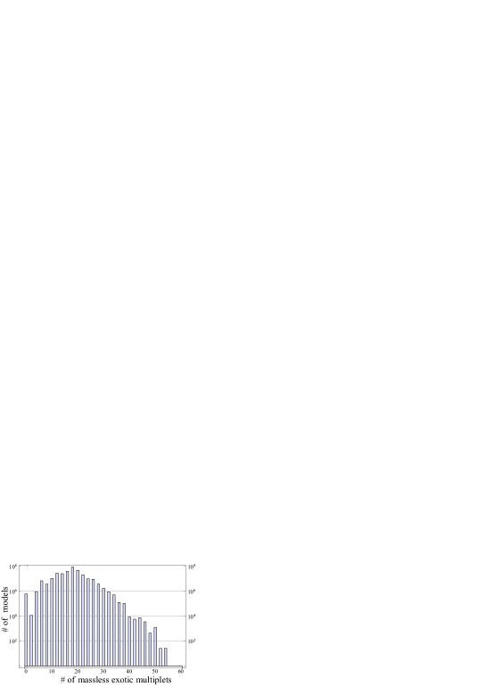
Figure 1: Number of 3–generation models versus total number of exotic multiplets in a random sample of $10^{11}$ Pati-Salam configurations.

The striking observations is that while the Pati–Salam case admits exophobic three generation models in the flipped $SU(5)$ case exophobic models with an odd number of generations do not appear. While positive confirmation, like the existence of a three generation exophobic model in the Pati–Salam case, is easy to verify, understanding their absence in the flipped $SU(5)$ case is more challenging. For example, it may merely reflect their absence in the particular space sampled. Nevertheless, the results shown in figures 1 and 2 exemplify the power of the classification methodology in extracting properties of large spaces of string vacua. Using the random generation of GGSO phases and imposing some prior criteria we can “fish” out models with desirable characteristics, provided that the statistical sample of the models with the required properties is not too small.

8 “Trolling” a model

A set of phases giving rise to a model with the desired properties is displayed in eq. (54). As advertised the observable gauge symmetry in this model is $SO(6)\times SO(4)\times U(1)_{1,2,3}$ and the family universal combination, $U(1)_{\zeta}=U(1)_{1}+U(1)_{2}+U(1)_{3}$, is anomaly free. The complete massless spectrum, as well as the cubic level superpotential are derived in ref. [38]. The massless chiral spectrum in the model appears in complete $27$ representations of $E_{6}$ decomposed under the effective observable gauge group, i.e. the chiral spectrum is self–dual under the spinor–vector duality. The model contains three chiral generations, as well as the required heavy and light Higgs states to produce a realistic fermion mass spectrum. Furthermore, the model admits a top quark mass term at the cubic level of the superpotential, i.e. $\lambda_{t}\sim 1$ in the model. A VEV of the heavy Higgs field that breaks the Pati–Salam symmetry to the Standard Model along flat directions leaves the unbroken combination

$$U(1)_{Z^{\prime}}~{}~{}=~{}~{}{1\over 5}~{}U(1)_{C}~{}~{}-~{}~{}{1\over 5}~{}U(1)_{L}-U_{\zeta}.$$ (53)

This $U(1)$ symmetry may remain unbroken down to low scales as it is anomaly free in this model.

$$(v_{i}|v_{j})\ \ =\ \ \bordermatrix{&1&S&e_{1}&e_{2}&e_{3}&e_{4}&e_{5}&e_{6}&b_{1}&b_{2}&z_{1}&z_{2}&\alpha\cr 1&1&1&1&1&1&1&1&1&1&1&1&1&1\cr S&1&1&1&1&1&1&1&1&1&1&1&1&1\cr e_{1}&1&1&0&0&0&0&0&0&0&0&0&0&1\cr e_{2}&1&1&0&0&0&0&0&1&0&0&0&1&0\cr e_{3}&1&1&0&0&0&1&0&0&0&0&0&1&1\cr e_{4}&1&1&0&0&1&0&0&0&0&0&1&0&0\cr e_{5}&1&1&0&0&0&0&0&1&0&0&0&1&1\cr e_{6}&1&1&0&1&0&0&1&0&0&0&1&0&0\cr b_{1}&1&0&0&0&0&0&0&0&1&1&0&0&0\cr b_{2}&1&0&0&0&0&0&0&0&1&1&0&0&1\cr z_{1}&1&1&0&0&0&1&0&1&0&0&1&1&0\cr z_{2}&1&1&0&1&1&0&1&0&0&0&1&1&0\cr\alpha&1&1&1&0&1&0&1&0&1&0&1&0&1\cr}$$ (54)

We note that maintaining the $U(1)_{Z^{\prime}}$ symmetry in eq. (53) unbroken down to low scales, requires the existence of additional matter states down to the $U(1)_{Z^{\prime}}$ breaking scale. Existence of this $U(1)$ symmetry at this scale will be accompanied by additional states with specific Standard Model and $U(1)_{Z^{\prime}}$ charges, which are mandated by anomaly cancellation and are compatible with the charge assignments in the string model. The string models give rise to a variety of Standard Model extensions, and each case is accompanied by specific additional states, which leads to unique signatures [25].

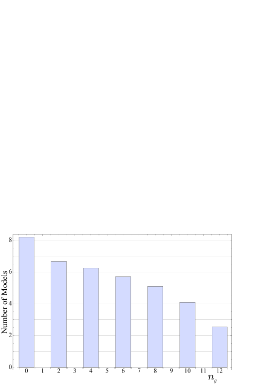
Figure 2: Number of exophobic models versus the number of generations in a random sample of $10^{12}$ flipped $SU(5)$ configurations.

An additional type of states that are of interest in this model are states that are $SO(10)$ singlets with non–standard $U(1)_{\zeta}$ charges. Such states are standard states with respect to the Standard Model charges, but are exotic states with respect to $E_{6}$. They arise from the breaking of $E_{6}$ in the string model by Wilson lines, and fall into the general category of Wilsonian matter states discussed in ref. [39]. They may play the role of dark matter candidates. Breaking the $U(1)_{Z^{\prime}}$ symmetry with states carry the standard conventional $E_{6}$ charges, leaves a remnant discrete symmetry that forbids the decay of the lightest exotic state to the lighter states [39]. The exotic states in this model are particularly appealing because they are Standard Model, and in fact $SO(10)$, singlets.

9 Conclusions

The available observational data at accessible energy scales favour the high scale unification of the gauge interactions and matter representations in Grand Unified Theories. Gravity is left out of this picture, and it is anticipated that may of the properties of the Standard Model particles, like the origin of their masses, can only be determined if gravity is incorporated into the fold. However, point quantum field theories have not led to a consistent synthesis with gravity, and it may well be that consistent unification of gravity with the gauge interactions requires a departure from the point particle idealisation. Contemporary string theories therefore provide a concrete framework to explore the unification of gravity and the gauge interactions.

In this paper we discussed the construction of string derived models that allow for the existence of an extra $U(1)$ symmetry at low scales. While the phenomenological analysis of such symmetries received ample attention in the literature, the construction of heterotic–string models that allow for a light $Z^{\prime}$ gauge boson has proven to be problematic. One of the main difficulties being that the desired symmetries tend to be anomalous in the string derived models and are broken at the high scale. For this purpose we utilised the classification methodology developed in the free fermionic formulation. We used the self–duality property under the spinor–vector duality to construct a string model in which the $E_{6}$ symmetries are anomaly free. This is obtained because due to the self–duality property, the chiral spectrum arises in complete $27$ representations of $E_{6}$. However, the remarkable point is that the gauge symmetry is not enhanced to $E_{6}$, but remains a subgroup of anomaly free $SO(10)\times U(1)_{\zeta}$. This is possible because the different components in the $27$ representations are obtained from different fixed points of the $Z_{2}\times Z_{2}$ orbifold. It is further noted that while our exemplary model is free of exotic fractionally charged massless states, it contains states that carry exotic states with respect to $U(1)_{\zeta}$, which are natural dark matter candidates. It will be of further interest to explore whether similar characteristics can be obtained in other classes of heterotic–string compactifications [40].

10 Acknowledgments

AEF would like to thank the University of Oxford and CERN for hospitality. AEF is supported in part by STFC under contract ST/L000431/1. This research has been co-financed by the European Union (European Social Fund - ESF) and Greek national funds through the Operational Program “Education and Lifelong Learning” of the National Strategic Reference Framework (NSRF) - Research Funding Program: THALIS Investing in the society of knowledge through the European Social Fund.

References

-
[1]
H. Kawai, D.C. Lewellen, and S.H.-H. Tye,
Nucl. Phys. B288 (1987) 1;
I. Antoniadis, C. Bachas, and C. Kounnas, Nucl. Phys. B289 (1987) 87;
I. Antoniadis and C. Bachas, Nucl. Phys. B289 (1987) 87. -
[2]
A.E. Faraggi, D.V. Nanopoulos and K. Yuan,
Nucl. Phys. B335 (1990) 347;
G.B. Cleaver, A.E. Faraggi and D.V. Nanopoulos, Phys. Lett. B455 (1999) 135. - [3] K. Christodoulides, A.E. Faraggi and J. Rizos, Phys. Lett. B702 (2011) 81.
- [4] A.E. Faraggi, Phys. Lett. B274 (1992) 47; Phys. Lett. B377 (1996) 43.
-
[5]
J. Rizos and K. Tamvakis, Phys. Lett. B279 (1992) 281;
A.E. Faraggi, Nucl. Phys. B407 (1993) 57; Nucl. Phys. B487 (1997) 55;
A.E. Faraggi and E. Halyo, Phys. Lett. B307 (1993) 305; Nucl. Phys. B416 (1994) 63. -
[6]
I. Antoniadis, J. Rizos and K. Tamvakis,
Phys. Lett. B279 (1992) 281;
A.E. Faraggi, Phys. Lett. B245 (1990) 435;
A.E. Faraggi and E. Halyo, Phys. Lett. B307 (1993) 311;
C. Coriano and A.E. Faraggi, Phys. Lett. B581 (2004) 99. -
[7]
A.E. Faraggi, Phys. Lett. B302 (1993) 202;
K.R. Dienes and A.E. Faraggi, Phys. Rev. Lett. 75 (1995) 2646; Nucl. Phys. B457 (1996) 409. - [8] A.E. Faraggi, Nucl. Phys. B428 (1994) 111; Phys. Lett. B520 (2001) 337.
- [9] A.E. Faraggi and J.C. Pati, Nucl. Phys. B526 (1998) 21.
- [10] A.E. Faraggi, Nucl. Phys. B728 (2005) 83.
-
[11]
A.E. Faraggi, C. Kounnas, S.E.M. Nooij and J. Rizos, Nucl. Phys. B695 (2004) 41;
A.E. Faraggi, C. Kounnas and J. Rizos, Phys. Lett. B648 (2007) 84. - [12] B. Assel, K. Christodoulides, C. Kounnas and J. Rizos, Phys. Lett. B683 (2010) 306; Nucl. Phys. B844 (2011) 365.
- [13] A.E. Faraggi, J. Rizos and H. Sonmez, Nucl. Phys. B886 (2014) 202.
-
[14]
A.E. Faraggi, C. Kounnas and J. Rizos, Nucl. Phys. B774 (2007) 208;
Nucl. Phys. B799 (2008) 19;
T. Catelin–Jullien, A.E. Faraggi, C. Kounnas and J. Rizos, Nucl. Phys. B812 (2009) 103;
C. Angelantonj, A.E. Faraggi and M. Tsulaia, JHEP 1007 (2010) 004. - [15] A.E. Faraggi, I. Florakis, T. Mohaupt and M. Tsulaia, Nucl. Phys. B848 (2011) 332.
- [16] L. Ibanez and A. Uranga, String theory and particle physics: an introduction to string phenomenology, Cambridge University Press, 2012.
- [17] A.E. Faraggi and D.V. Nanopoulos, Mod. Phys. Lett. A6 (1991) 61.
- [18] J.C. Pati, Phys. Lett. B388 (1996) 532.
- [19] A.E. Faraggi, Phys. Lett. B278 (1992) 131; Nucl. Phys. B387 (1992) 239.
- [20] A.E. Faraggi, Phys. Lett. B499 (2001) 147.
- [21] C. Coriano, A.E. Faraggi and M. Guzzi, Eur. Phys. Jour. C53 (2008) 421; Phys. Rev. D78 (2008) 015012.
- [22] D. Chang and A. Kumar, Phys. Rev. D38 (1988) 1893; Phys. Rev. D38 (1988) 3734.
- [23] A.E. Faraggi and D.V. Nanopoulos, Phys. Rev. D48 (1993) 3288.
-
[24]
G. Aad et al. [ATLAS Collaboration],
arXiv:1506.00962;
V. Khachatryan et al. [CMS Collaboration], JHEP 1408 (2014) 173;
V. Khachatryan et al. [CMS Collaboration], JHEP 1408 (2014) 174. -
[25]
A.E. Faraggi and M. Guzzi, arXiv:1507:07406;
T. li, J.A. Maxin, V.E. Mayes and D.V. Nanopoulos, arXiv:1509.06821. -
[26]
G.B. Cleaver, A.E. Faraggi and C. Savage, Phys. Rev. D63 (2001) 066001;
G.B. Cleaver, D.J. Clements and A.E. Faraggi, Phys. Rev. D65 (2002) 106003; - [27] A.E. Faraggi and V. Mehta, Phys. Rev. D84 (2011) 086006; Phys. Rev. D88 (2013) 025006.
-
[28]
I. Antoniadis, J. Ellis, J. Hagelin and D.V. Nanopoulos
Phys. Lett. B231 (1989) 65;
-
[29]
I. Antoniadis, G.K. Leontaris and J. Rizos,
Phys. Lett. B245 (1990) 161;
G.K. Leontaris and J. Rizos, Nucl. Phys. B554 (1999) 3. - [30] G.B. Cleaver and A.E. Faraggi, Int. J. Mod. Phys. A14 (1999) 2335.
- [31] L. Bernard, A.E. Faraggi, I. Glasser, J. Rizos and H. Sonmez, Nucl. Phys. B868 (2013) 1.
- [32] P. Athanasopoulos, A.E. Faraggi and V. Mehta, Phys. Rev. D89 (2014) 105023.
- [33] A. Giveon, M. Porrati and E. Rabinovici, Phys. Rep. 244 (1994) 77.
- [34] B.R. Greene and M.R. Plesser, Nucl. Phys. B338 (1990) 15.
- [35] D. Gepner, Phys. Lett. B199 (1987) 380; Nucl. Phys. B296 (1988) 757.
- [36] P. Athanasopoulos, A.E. Faraggi and D. Gepner, Phys. Lett. B735 (2014) 357.
- [37] A. Gregori, C. Kounnas and J. Rizos, Nucl. Phys. B549 (1999) 16.
- [38] A.E. Faraggi and J. Rizos, Nucl. Phys. B895 (2015) 233.
- [39] S. Chang, C. Coriano and A.E. Faraggi, Nucl. Phys. B477 (1996) 65.
-
[40]
B. Greene, K. Kirklin, P. Miron and G.G. Ross,
Nucl. Phys. B278 (1986) 667;
L. Ibanez, J.E. Kim, P. Nilles, F. Quevedo, Phys. Lett. B191 (1987) 282;
D. Gepner, hep-th/9301089;
T. Kobayashi, S. Raby and R. Zhang, Nucl. Phys. B704 (2005) 3;
O. Lebedev et al, Phys. Lett. B645 (2007) 88;
M. Blaszczyk et al, Phys. Lett. B683 (2010) 340;
B. Gato–Rivera, A. Schellekens, Nucl. Phys. B828 (2010) 375.