The Networked Partial Correlation and its Application to the Analysis of Genetic Interactions

Abstract

Genetic interactions confer robustness on cells in response to genetic perturbations. This often occurs through molecular buffering mechanisms that can be predicted using, among other features, the degree of coexpression between genes, commonly estimated through marginal measures of association such as Pearson or Spearman correlation coefficients. However, marginal correlations are sensitive to indirect effects and often partial correlations are used instead. Yet, partial correlations convey no information about the (linear) influence of the coexpressed genes on the entire multivariate system, which may be crucial to discriminate functional associations from genetic interactions. To address these two shortcomings, here we propose to use the edge weight derived from the covariance decomposition over the paths of the associated gene network. We call this new quantity the networked partial correlation and use it to analyze genetic interactions in yeast.

Keywords: Covariance decomposition; Concentration matrix; Gene coexpression; Partial correlation; Undirected graphical model.

1 Introduction

The deletion of individual genes in model organisms, such as the budding yeast, Saccharomyces cerevisiae, produces mutants that cannot express the knocked-out gene, constituting one of the primary tools in experimental genetics to elucidate gene function. However, the systematic culture of yeast single-gene mutants has revealed that the majority of its about 6000 genes are dispensable because no sizable effect in fitness can be observed among the corresponding mutants (Winzeler et al., 1999). An explanation to this observation is the presence of buffering relationships between pairs of genes, by which the absence of one gene is counterbalanced by the expression of its partner. The simultaneous deletion of two genes produces a so-called double mutant organism. When the change in fitness of a double-mutant significantly deviates from the expected change resulting from the combination of the two single mutant fitness effects, then one concludes that there is a so-called genetic interaction between these two genes. A reduction in fitness by a double-mutant is known as synthetic sickness and the extreme case of this phenomenon, which is known as synthetic lethality, occurs when two single mutants are still viable but the genetic interaction of the two knocked-out genes leads to cell death (Tucker and Fields, 2003). This concept has been exploited in the field of cancer research to tackle the resistance to chemotherapeutics by trying to target multiple oncogenes simultaneously (Luo et al., 2009; Jerby-Arnon et al., 2014).

Genetic interactions can be experimentally identified in a number of ways. One of them consists of measuring the deviation in fitness between the expected effect of combining two single mutants and the observed effect of the corresponding double mutant (Baryshnikova et al., 2010). Yet, producing an exhaustive catalogue of single and double mutants to enable the exploration of all possible genetic interactions is only feasible in model organisms with a moderate number of genes, such as yeast. For this reason, it is important to have computational tools that enable predicting genetic interactions in larger model organisms (Eddy, 2006) and, ideally, in humans (Deshpande et al., 2013) where, in addition to the reduced possibilities for genetic manipulation, the number of possible gene pairs can be tenfold larger.

The simultaneous expression of two genes, known as gene coexpression, is a proxy for the presence of a functional association between them. The high-throughput profiling of expression for thousands of genes in parallel provides multivariate data whose analysis with clustering techniques and graphical models has proven to be useful for exploring gene coexpression in terms of gene network representations of the data. This has been exploited in a number of applications ranging from inferring function in poorly characterized genes to predicting buffering relationships behind genetic interactions (Eisen et al., 1998; Friedman, 2004; Wong et al., 2004; Jerby-Arnon et al., 2014). Existing approaches that attempt to predict genetic interactions not only use gene coexpression but also many other biological features such as protein function and localization, homology relationships and protein-protein interactions (Wong et al., 2004; Zhong and Sternberg, 2006; Conde-Pueyo et al., 2009; Deshpande et al., 2013; Jerby-Arnon et al., 2014), which we will not consider in this paper.

Gene coexpression is commonly identified using Pearson or Spearman correlation coefficients. However, the marginal nature of these quantities often leads to spurious associations resulting from indirect effects and nonbiological sources of variation. To address this problem, we can use graphical Gaussian models (Dempster, 1972; Whittaker, 1990) in which a key role is played by the partial covariance because if a pair of variables is not joined by an edge in the network, then the corresponding partial covariance is equal to zero. The partial covariance can be normalized to obtain a partial correlation that, in the molecular context, can be regarded as the natural measure of the strength of the direct association between the two genes forming an edge in the network (De La Fuente et al., 2004; Castelo and Roverato, 2006; Zuo et al., 2014). However, although partial correlation is a measure of direct coexpression between genes, the buffering mechanism behind a genetic interaction not only leads to gene coexpression but also confers robustness on the whole system in response to genetic perturbations (Nijman, 2011). From this perspective, the information that is provided by the value of a partial correlation is not sufficient to capture such a robustness, reflected in the functional relationship between the two intervening genes and the remaining genes in the system.

One of the first attempts to describe the influence of a direct association within an entire multivariate system was provided by Wright (1921), who described the covariance decomposition between two variables along their connecting paths in a directed graph (see also Chen and Pearl, 2015, for a recent review). More recently, within the analysis of undirected graphical Gaussian models, Jones and West (2005) showed how the covariance between two variables can be computed as the sum of weights associated with the undirected paths joining the variables, providing the undirected counterpart to the results of Wright (1921). In this paper, we make the observation that every single edge in a network can be regarded as a path, and therefore, can also have such a weight associated with it. We investigate how that weight captures both the strength of the direct association between the two variables and their relationship with the remaining variables in the system. We provide an interpretation of these edge weights that suggests us to name them networked partial covariances and then we normalize them to obtain networked partial correlations. We demonstrate how the covariance turns out to be a special case of the networked partial covariance, and how this result generalizes the covariance decomposition of Jones and West (2005). Finally, we demonstrate how networked partial correlations improve marginal and partial correlations as proxies for the presence of buffering relationships behind genetic interactions in yeast.

This paper is organized as follows. Section 2 provides the required background on undirected graphical models, path weights and the partial vector correlation coefficient. In Section 3 the definitions of the networked partial covariance and correlation are given and their interpretation discussed. The limited-order networked partial covariance and its decomposition are given in Section 4. Section 5 presents the results on the analysis of genetic interactions in yeast whereas in the Supplementary Material we provide full details on how the data were analysed. Finally, Section 6 contains a discussion.

2 Notation and background

2.1 Undirected graphical models

Let $\mathbf{X}\equiv\mathbf{X}_{V}$ be a random vector indexed by a finite set $V=\{1,\ldots,p\}$ so that for $A\subseteq V$, $\mathbf{X}_{A}$ is the subvector of $\mathbf{X}$ indexed by $A$. The random vector $\mathbf{X}_{V}$ has probability distribution $\mathbb{P}_{V}$ and we denote the covariance matrix of $\mathbf{X}_{V}$ by $\varSigma=\varSigma_{VV}=\{\sigma_{uv}\}_{u,v\in V}$ and the concentration (or precision) matrix by $\varSigma^{-1}=\mathit{K}=\{\kappa_{uv}\}_{u,v\in V}$. For $B\subseteq V$ with $A\cap B=\emptyset$ the partial covariance matrix $\varSigma_{AA\cdot B}=\varSigma_{AA}-\varSigma_{AB}\varSigma_{BB}^{-1}\varSigma_{BA}$ is the covariance matrix of $\mathbf{X}_{A}|\mathbf{X}_{B}$, that is the residual vector deriving from the linear least square predictor of $\mathbf{X}_{A}$ from $\mathbf{X}_{B}$ (see Whittaker, 1990, p. 134). Recall that, in the Gaussian case, $\varSigma_{AA\cdot B}$ coincides with the covariance matrix of the conditional distribution of $\mathbf{X}_{A}$ given $\mathbf{X}_{B}$. We use the convention that we write $\varSigma_{AA}^{-1}$ when the submatrix extraction is performed before the inversion, that is $\varSigma_{AA}^{-1}=(\varSigma_{AA})^{-1}$ and, similarly, $\varSigma_{AA\cdot B}^{-1}=(\varSigma_{AA\cdot B})^{-1}$. We write $\bar{A}=V\backslash A$ to denote the complement of a subset $A$ with respect to $V$ and recall that, from the rule for the inversion of a partitioned matrix, $\varSigma_{AA\cdot\bar{A}}^{-1}=\mathit{K}_{AA}$ and, accordingly, $\varSigma_{AA}^{-1}=\mathit{K}_{AA\cdot\bar{A}}$.

An undirected graph with vertex set $V$ is a pair $\mathcal{G}=(V,\mathcal{E})$ where $\mathcal{E}$ is a set of edges, which are unordered pairs of vertices; formally $\mathcal{E}\subseteq V\times V$. The graphs we consider have no self-loops, that is $\{v,v\}\not\in\mathcal{E}$ for any $v\in V$. The subgraph of $\mathcal{G}$ induced by $A\subseteq V$ is the undirected graph $\mathcal{G}_{A}$ with vertex set $A$ and edges $\mathcal{E}_{A}=\{\{u,v\}\in\mathcal{E}:u,v\in A\}$. A path between $x$ and $y$ in $\mathcal{G}$ is a sequence $\pi=\langle x=v_{1},\ldots,v_{k}=y\rangle$ of $k\geq 2$ distinct vertices such that $\{v_{i},v_{i+1}\}\in\mathcal{E}$ for every $i=1,\ldots,k-1$ and we denote by $\Pi_{xy}$ the collection of all paths from $x$ to $y$ in $\mathcal{G}$. We denote by $V(\pi)\subseteq V$ and $\mathcal{E}(\pi)\subseteq\mathcal{E}$ the set of vertices and edges of the path $\pi$, respectively. When clear from the context, and to improve the readability of sub- and super-scripts, we will set $P\equiv V(\pi)$.

We say that the concentration matrix $\mathit{K}$ of $\mathbf{X}_{V}$ implies the graph $\mathcal{G}=(V,\mathcal{E})$ if every nonzero off-diagonal entry of $\mathit{K}$ corresponds to an edge in $\mathcal{G}$. The concentration graph model (Cox and Wermuth, 1996) with graph $\mathcal{G}$ is the family of multivariate normal distributions whose concentration matrix implies $\mathcal{G}$. The latter model has also been called a covariance selection model (Dempster, 1972) and a graphical Gaussian model (Whittaker, 1990); we refer the reader to Lauritzen (1996) for details and discussion on this type of model.

2.2 Path weights

Let $V$ be a finite set and $\mathcal{G}=(V,\mathcal{E})$ be an undirected graph. Furthermore, let $\pi$ be a path from $x$ to $y$ in $\mathcal{G}$ and $\varGamma\equiv\varGamma_{VV}$ a positive definite matrix indexed by the elements of V. We set

$$\omega(\pi,\varGamma) \equiv (-1)^{|P|+1}\;|\varGamma_{PP}|\;\prod_{\{u,v\}\in\mathcal{E}(\pi)}\{\varGamma^{-1}\}_{uv}\,,$$ (1)

where $|P|$ denotes the cardinality of $P=V(\pi)$ whereas $|\varGamma_{PP}|$ is the determinant of $\varGamma_{PP}$. Jones and West (2005) introduced (1) in an alternative formulation that relies on the equality

$$|\varGamma_{PP}|=\frac{|\varTheta_{\bar{P}\bar{P}}|}{|\varTheta|}$$ (2)

where $\varTheta=\varGamma^{-1}$, and with the convention that $|\varTheta_{\bar{P}\bar{P}}|=1$ whenever $\bar{P}=\emptyset$.

Theorem 2.1 (Jones and West (2005)).

Let $\mathit{K}=\varSigma^{-1}$ be the concentration matrix of $\mathbf{X}_{V}$. If $\mathit{K}$ implies the graph $\mathcal{G}=(V,\mathcal{E})$ then for every $x,y\in V$ it holds that

$$\sigma_{xy}=\sum_{\pi\in\Pi_{xy}}\omega(\pi,\varSigma)=\sum_{\pi\in\Pi_{xy}}(-1)^{|P|+1}\;\frac{|\mathit{K}_{\bar{P}\bar{P}}|}{|\mathit{K}|}\;\prod_{\{u,v\}\in\mathcal{E}(\pi)}\kappa_{uv}.$$ (3)

We call $\omega(\pi,\varSigma)$ in (3) the path weight of $\pi$ relative to $\mathbf{X}_{V}$. Furthermore, we will refer to (3) with the name of the covariance decomposition over $\mathcal{G}$ because it gives a decomposition of $\sigma_{xy}$ into the sum of the path weights for all the paths connecting the two vertices in $\mathcal{G}$. We recall that another interesting decomposition of the covariance in Gaussian models in terms of walk-weights can be found in Malioutov et al. (2006) and references therein. Unlike paths, walks can cross an edge multiple times.

2.3 The partial vector correlation coefficient

We denote by $\rho_{xy}$ the correlation coefficient of the variables $X_{x}$ and $X_{y}$, with $x,y\in V$. Furthermore, we write $\rho_{xy\cdot V\backslash\{x,y\}}$ to denote the partial correlation coefficient of $X_{x}$ and $X_{y}$ given $\mathbf{X}_{V\backslash\{x,y\}}$, and recall that (Lauritzen, 1996, p. 130)

$$\rho_{xy\cdot V\backslash\{x,y\}}=\frac{-\kappa_{xy}}{\sqrt{\kappa_{xx}\kappa_{yy}}}\,.$$ (4)

In the literature, different quantities have been introduced to provide a generalization of the concept of (partial) correlation from pairs of variables to pairs of vectors; see Robert and Escoufier (1976), Mardia et al. (1979, Section 6.5.4), Timm (2002, p. 485) and Kim and Timm (2006, Section 5.6) for a review of measures of correlation between vectors. The rest of this section is devoted to a coefficient, called the partial vector correlation, which plays a central role in this paper because it naturally arises in the theory of path weights. As shown below, this coefficient can be obtained as a function of certain canonical correlations and this can be used to assess its connections with other more common measures of association between vectors such as, for instance, the RV-coefficient (see Robert and Escoufier, 1976, for details).

For a pair $A,B\subseteq V$, with $A\cap B=\emptyset$, Hotelling (1936) introduced the vector alienation coefficient defined as $\lambda_{(A)(B)}\equiv|\varSigma_{A\cup BA\cup B}|/\left(|\varSigma_{AA}|\times|\varSigma_{BB}|\right)$. Notice that the sampling version of $\lambda_{(A)(B)}$ is the Wilks’ lambda, used to test the independence of $\mathbf{X}_{A}$ and $\mathbf{X}_{B}$ under normality. Furthermore,

$$\lambda_{(A)(B)}=\prod_{i=1}^{r}(1-\varrho_{i}^{2})\,,$$ (5)

where $\varrho_{i}$, for $i=1,\ldots,r$, is the $i$-th canonical correlation between $\mathbf{X}_{A}$ and $\mathbf{X}_{B}$ and $r=\min(|A|,|B|)$; see Mardia et al. (1979, Section 6.5.4) and Timm (2002, p. 485).

The vector alienation coefficient was used by Rozeboom (1965) to define the vector correlation coefficient given by

$$\rho_{(A)(B)}\equiv\sqrt{1-\lambda_{(A)(B)}}\,,$$ (6)

and it is easy to check that, for $A=\{x\}$, $\rho^{2}_{(A)(B)}$ coincides with the square of the multiple correlation coefficient so that if also $B=\{y\}$ then $\rho_{(A)(B)}^{2}=\rho_{xy}^{2}$ (see also Timm, 2002, p. 485).

Consider a subset $C\subseteq V$ such that $A\cap C=B\cap C=\emptyset$. Rozeboom (1965) generalized (6) to the partial vector correlation coefficient as follows,

$$\rho_{(A)(B)\cdot C}=\sqrt{1-\lambda_{(A)(B)\cdot C}},\qquad\mbox{where}\qquad\lambda_{(A)(B)\cdot C}=\frac{|\varSigma_{A\cup BA\cup B\cdot C}|}{|\varSigma_{AA\cdot C}||\varSigma_{BB\cdot C}|}.$$ (7)

We remark that the covariance matrices we consider are assumed to be positive definite so that $0\leq\rho_{(A)(B)\cdot C}<1$. Furthermore, $\rho_{(A)(B)}=\rho_{(A)(B)\cdot\emptyset}$, and we use the convention that $\rho_{(A)(B)\cdot C}=0$ whenever either $A=\emptyset$ or $B=\emptyset$. Note that, for $A=\{x\}$ and $B=\{y\}$ it holds that $\rho_{(A)(B)\cdot C}^{2}=\rho_{xy\cdot C}^{2}$ that is the square of the partial correlation.

3 Networked partial covariance and correlation

The decomposition of the covariance $\sigma_{xy}$ over an undirected graph in (3) associates a weight to every path $\pi$ between $x$ and $y$ in $\mathcal{G}$. Hence, the weight $\omega(\pi,\varSigma)$ represents the contribution of the path $\pi$ to the covariance $\sigma_{xy}$ and from this perspective it is appealing to investigate this quantity as a measure of association between $X_{x}$ and $X_{y}$. However, one cannot readily exploit the covariance decomposition over paths because the interpretation of path weights is unclear and is still an open problem. More specifically, it follows from equation (4) that the term $(-1)^{|P|+1}$ in equation $(\ref{EQN:in.thm.jones.west})$ is such that $\omega(\pi,\varSigma)$ has the same sign as the product of the partial correlations corresponding to the edges of the path but, otherwise, it is not clear what the meaning is of the value taken by a path weight. In this section, we address this question by focusing on the special and relevant case of single-edge paths, which are paths made of a single edge.

If an edge is missing from the graph $\mathcal{G}$, say $\{x,y\}\not\in\mathcal{E}$, then the corresponding partial covariance is equal to zero, $\sigma_{xy\cdot V\backslash\{x,y\}}=0$, and for this reason partial covariances and partial correlations are regarded as natural measures to be associated with the edges of the graph. The following theorem shows that the weight $\omega(\langle x,y\rangle,\varSigma)$ of a single-edge path $\langle x,y\rangle$ is a quantity that involves not only the partial covariance associated with the edge, but also a vector correlation coefficient.

Theorem 3.1.

Let $\mathit{K}=\varSigma^{-1}$ be the concentration matrix of $\mathbf{X}_{V}$. If $\mathit{K}$ implies the graph $\mathcal{G}=(V,\mathcal{E})$, then for every $\{x,y\}\in\mathcal{E}$ it holds that

$$\omega(\langle x,y\rangle,\varSigma) = \frac{\sigma_{xy\cdot V\backslash\{x,y\}}}{1-\rho^{2}_{(xy)(V\backslash\{x,y\})}},$$ (8)

where we have used the suppressed notation $\rho_{(xy)(B)}=\rho_{(\{x,y\})(B)}$.

Proof.

See Appendix A ∎

In what follows, we denote the weight of the single-edge path $\langle x,y\rangle$ more compactly as

$$\omega_{xy\cdot(V\backslash\{x,y\})}\equiv\omega(\langle x,y\rangle,\varSigma)$$

and refer to this quantity as a networked partial covariance. When the edge $\{x,y\}$ is missing, $\sigma_{xy\cdot V\backslash\{x,y\}}=0$ and, therefore, $\omega_{xy\cdot(V\backslash\{x,y\})}=0$. Moreover, $\omega_{xy\cdot(V\backslash\{x,y\})}$ and $\sigma_{xy\cdot V\backslash\{x,y\}}$ have the same sign, and $|\omega_{xy\cdot(V\backslash\{x,y\})}|\geq|\sigma_{xy\cdot V\backslash\{x,y\}}|$.

Furthermore, the ratio in equation (8) provides a clear interpretation of the edge weight $\omega_{xy\cdot(V\backslash\{x,y\})}$ because it shows that $\omega_{xy\cdot(V\backslash\{x,y\})}$ is obtained by combining the information that is provided by $\sigma_{xy\cdot V\backslash\{x,y\}}$ and $\rho_{(xy)(V\backslash\{x,y\})}$. More concretely, the networked partial covariance is computed by multiplying the partial covariance $\sigma_{xy\cdot V\backslash\{x,y\}}$ by $1/\{1-\rho_{(xy)(V\backslash\{x,y\})}\}$, which is always greater than or equal to 1 and an increasing function of $\rho_{(xy)(V\backslash\{x,y\})}$. Furthermore, it is worth noticing that $\sigma_{xy\cdot V\backslash\{x,y\}}$ and $\rho_{(xy)(V\backslash\{x,y\})}$ provide two distinct pieces of information.

1. The information provided by $\sigma_{xy\cdot V\backslash\{x,y\}}$ concerns the presence of the edge $\{x,y\}$ in $\mathcal{G}=(V,\mathcal{E})$ because $\sigma_{xy\cdot V\backslash\{x,y\}}\neq 0$ implies $\{x,y\}\in\mathcal{E}$. More concretely, it equals the covariance of $X_{x}$ and $X_{y}$ computed after the two variables have been linearly adjusted for the remaining variables in the network. Hence, $\sigma_{xy\cdot V\backslash\{x,y\}}$ provides no information on the strength of the linear association between $X_{x}$ and $X_{y}$ and the remaining variables in the network. In other words, $\sigma_{xy\cdot V\backslash\{x,y\}}$ can be regarded as an ‘outer’ measure of the association encoded by the edge $\{x,y\}$, because the way in which $\{x,y\}$ is connected with the rest of the network, plays no role in its computation. This kind of interpretation is even stronger in the case where the variables are jointly Gaussian, because in this case $\sigma_{xy\cdot V\backslash\{x,y\}}$ is the covariance of the conditional distribution of $\mathbf{X}_{\{x,y\}}|\mathbf{X}_{V\backslash\{x,y\}}$.

2. The vector correlation $\rho_{(xy)(V\backslash\{x,y\})}$ is a measure of the strength of the association between $\mathbf{X}_{\{x,y\}}$ and the remaining variables $\mathbf{X}_{V\backslash\{x,y\}}$, and provides no information on whether $x$ and $y$ are joined by an edge. Regardless of whether $\{x,y\}$ is an edge of the graph, when the pair $\{x,y\}$ is disconnected from the rest of the network then $\rho_{(xy)(V\backslash\{x,y\})}=0$ and, consequently, $\omega_{xy\cdot(V\backslash\{x,y\})}=\sigma_{xy\cdot V\backslash\{x,y\}}$.

In summary, the weight $\omega_{xy\cdot(V\backslash\{x,y\})}$ synthesizes in a single quantity the strength of the partial covariance between $X_{x}$ and $X_{y}$, and the strength of the vector correlation between $X_{\{x,y\}}$ and the remaining variables in the network. This interpretation motivates the name of networked partial covariance.

Just as covariances need to be normalized into correlations to enable their comparison, we provide also the normalized version of equation (8) that we shall call the networked partial correlation:

$$\psi_{xy\cdot(V\backslash\{x,y\})}\equiv\frac{\omega_{xy\cdot(V\backslash\{x,y\})}}{\sqrt{\sigma_{xx\cdot V\backslash\{x,y\}}\,\sigma_{yy\cdot V\backslash\{x,y\}}}}=\frac{\rho_{xy\cdot V\backslash\{x,y\}}}{1-\rho^{2}_{(xy)(V\backslash\{x,y\})}}\,.$$ (9)

Although expression (9) is a normalized quantity and, therefore, comparable between edges from the same graph, it may take values outside the interval $[-1,1]$. The following example gives a simplified setting that makes it clear how the networked partial correlation can be regarded as an ‘inflated’ version of the partial correlation to keep into account how the edge is embedded in the network.

Example 3.1.

Consider the case where $|V|=9$ and the concentration matrix $\mathit{K}$ of $\mathbf{X}_{V}$ induces the graph $\mathcal{G}=(V,\mathcal{E})$ in Fig. 1.

Figure 1: Undirected graph of the Example 3.1. Values on the edges correspond to networked partial correlations.

More specifically, we take $\mathit{K}$ to have unit diagonal and off-diagonal elements $\kappa_{uv}=-0.4$ for every $\{u,v\}\in\mathcal{E}$ and $\kappa_{uv}=0$ otherwise. The simplified structure of the concentration matrix in this example makes it easy to appreciate the differences existing between partial correlations and networked partial correlations. Indeed, in this case, the partial correlations $\rho_{uv\cdot V\backslash\{u,v\}}$ for $\{u,v\}\in\mathcal{E}$ put all the edges of the graph on an equal footing because they are all equal to $0.4$. However, the networked partial correlations, whose values are reported in Fig. 1, are not constant and, in this case, their differences depend only on the structure of the graph. Indeed, the edge $\{8,9\}$ is disconnected from the rest of the vertices so that the values of its networked partial correlation and partial correlation coincide; i.e. $\psi_{89\cdot(V\backslash\{8,9\})}=\rho_{89\cdot V\backslash\{8,9\}}=0.4$. The edge $\{4,5\}$ has the largest number of connections with other vertices in the graph and, accordingly, its networked partial correlation takes the largest value $\psi_{45\cdot(V\backslash\{4,5\})}=1.7$. More generally, in this example, the value of the networked partial correlation of every edge is proportional to the number of vertices adjacent to the edge.

4 Limited-order networked partial covariance decomposition

In practical applications, it is common to deal with limited-order partial covariances, which are partial covariances $\sigma_{xy\cdot Q}$ with $Q\cup\{x,y\}\subset V$, rather than with full-order partial covariances $\sigma_{xy\cdot V\backslash\{x,y\}}$. Typically, this is due to the presence of unobserved variables, possibly not explicitly considered in the analysis or because the number of variables exceeds the sample size, so that the sample covariance matrix has not full rank, thereby making the computation of full-order partial covariances unfeasible; see Castelo and Roverato (2006), Zuo et al. (2014) and references therein. In these cases, it is therefore also sensible to work with limited-order path weights rather than full-order path weights. Consider the concentration matrix $\mathit{K}=\varSigma^{-1}$ of $\mathbf{X}_{V}$ that implies the graph $\mathcal{G}=(V,\mathcal{E})$. For a subset $Q\subset V\backslash\{x,y\}$ we define the limited-order weight of the single-edge path $\langle x,y\rangle$ as the weight of $\langle x,y\rangle$ relative to $\mathbf{X}_{Q\cup\{x,y\}}$; formally $\omega_{xy\cdot(Q)}\equiv\omega(\langle x,y\rangle,\varSigma_{Q\cup\{x,y\}Q\cup\{x,y\}})$. Since it follows from Theorem 3.1 that

$$\omega_{xy\cdot(Q)} = \frac{\sigma_{xy\cdot Q}}{1-\rho^{2}_{(xy)(Q)}},$$ (10)

we refer to $\omega_{xy\cdot(Q)}$ as a limited-order networked partial covariance. For $Q=\emptyset$ it holds that $\omega_{xy\cdot(Q)}=\sigma_{xy.Q}=\sigma_{xy}$, and therefore, the (marginal) covariance can be regarded as a special case of both the limited-order partial covariance and the limited-order networked partial covariance. It follows from (10) that the limited-order networked partial correlation can be defined as

$$\psi_{xy\cdot(Q)}=\frac{\omega_{xy\cdot(Q)}}{\sqrt{\sigma_{xx\cdot Q}\,\sigma_{yy\cdot Q}}}=\frac{\rho_{xy\cdot Q}}{1-\rho^{2}_{(xy)(Q)}}.$$

To interpret the meaning of any limited-order quantity properly it is necessary to clarify how such quantity is affected by the marginalization over the variables that are excluded from the analysis. More specifically, when the relevant limited-order quantity is used to describe the association that is represented by an edge of the graph, then it is of interest to investigate what the role that is played by the structure of the full, unobserved, network $\mathcal{G}_{V}$ is in the specification of such a quantity. In the following theorem we give a rule to decompose a limited-order networked partial covariance $\omega_{xy\cdot(Q)}$ over the paths between $x$ and $y$ in $\mathcal{G}_{V\backslash Q}$. This clarifies what the information that is provided by a networked partial covariance is, thereby providing a theoretical justification for its use.

Theorem 4.1.

Let $\mathit{K}=\varSigma^{-1}$ be the concentration matrix of $\mathbf{X}_{V}$. If $\mathit{K}$ implies the graph $\mathcal{G}=(V,\mathcal{E})$ then for every $x,y\in V$ and $Q\subseteq V\backslash\{x,y\}$ it holds that

$$\omega_{xy\cdot(Q)} = \sum_{\pi\in\Pi_{xy};V(\pi)\subseteq V\backslash Q}\omega(\pi,\varSigma)\times(1-\rho^{2}_{(P\backslash\{x,y\})(Q)\cdot\{x,y\}})$$ (11)

where $P=V(\pi)$.

Proof.

See Appendix A ∎

First, when $Q=\emptyset$ equation (11) coincides with (3) so that the limited-order partial covariance decomposition in Theorem 4.1 includes, as a special case, the covariance decomposition of Jones and West (2005), given in Theorem 2.1. Second, for $Q=V\backslash\{x,y\}$ equation (11) simplifies to $\omega_{xy\cdot(V\backslash\{x,y\})}=\omega(\langle x,y\rangle,\varSigma)$. More generally, the decomposition of the limited-order networked partial covariance given in Theorem 4.1 enables us to understand the connection between the weight of a path in a graph derived from a multivariate distribution, and the weight of a path in a graph derived from a marginal distribution. Concretely, it shows that every path $\pi\in\Pi_{xy}$ such that $V(\pi)\cap Q=\emptyset$ contributes to the value of $\omega_{xy\cdot(Q)}$ with the proportion $1-\rho^{2}_{(P\backslash\{x,y\})(Q)\cdot\{x,y\}}$ of its weight $\omega(\pi,\varSigma)$. More importantly, a path between two vertices $x$ and $y$ contributes to the value of $\omega_{xy\cdot(Q)}$ only if all its vertices, except for $x$ and $y$, have been marginalized over. This means that any path with at least one endpoint not equal to $x$ or $y$, and any path between $x$ and $y$ involving at least one vertex in $Q$, plays no role in the computation of $\omega_{xy\cdot(Q)}$. To make the rules for limited-order networked partial covariance decomposition more concrete, Appendix B gives a detailed description of the case where $|V|=4$ and $|Q|=1$.

Because any networked partial covariance is a path weight, an appealing feature of equation (11) is that both the term $\omega_{xy\cdot(Q)}$ in the left hand side and the terms $\omega(\pi,\varSigma)$ in the right hand side are path weights. This confers consistency to equation (11) that can thus be regarded as a rule to update the weight of single-edge paths when the multivariate system is marginalized over some variables. This motivates the use of the networked partial covariance as a natural generalization of the covariance. From this viewpoint, it is also worth noting that, by multiplying the left- and right-hand side of (11) by $1-\rho^{2}_{(xy)(Q)}$, Theorem 4.1 can be restated to provide a rule to decompose $\sigma_{xy\cdot Q}$. However, consistency of interpretation between the left- and the right-side of the equation is lost in this case.

5 Analysis of genetic interactions in yeast

5.1 Data preparation and estimation methods

Costanzo et al. (2010) generated quantitative genetic interaction profiles in a systematic way for about 75% of all the genes in yeast, using a technique called synthetic genetic array (SGA) analysis. This technique enabled the quantification for 6,647,235 gene pairs in yeast of the fitness effect of a double mutant with respect to the expected effect calculated from the combination of two single mutants. This quantification was provided through the so-called SGA scores that also have an associated $p$-value that captures how reliable they are (Baryshnikova et al., 2010). This reliability is measured through a combination of the observed variation across four experimental replicates, with estimates of the background log-normal error distributions for the corresponding mutants (Baryshnikova et al., 2010; Costanzo et al., 2010). We downloaded those SGA scores and $p$-values and filtered them to discard pairs displaying a defective experimental procedure, such as a missing SGA score, or duplicated gene pairs with SGA scores of opposite sign. Between two SGA scores of the same sign produced by a duplicated gene pair, we kept the SGA score with lowest $p$-value as suggested in (Costanzo et al., 2010). After this filtering step, we kept 5,195,591 gene pairs involving 4457 genes. We used these 5 million SGA scores as gold-standard for the fitness effect of genetic interactions in yeast (see Supplementary Materials).

To demonstrate the usefulness of networked partial correlations in this context, we used gene expression data produced by Brem and Kruglyak (2005) from a cross between two yeast strains: a wild-type (RM11-1a) and a lab strain (BY4716). These two strains were crossed by Brem and Kruglyak (2005) to generate $n=112$ segregants whose gene expression was profiled with microarray chips. We downloaded and processed the resulting raw data as described in Tur et al. (2014) leading to a normalized gene expression data matrix formed by $p=6216$ genes and $n=112$ samples.

The calculation of the networked partial correlation from expression data between two given genes involves the estimation of two quantities (see equation (9)): (i) the partial correlation between these two genes; and (ii) the vector correlation between this pair of genes and the rest of the genes. Because the number of genes, $p$, is much larger than the number of samples, $n$, i.e., $p\gg n$, the calculation of these two quantities is not straightforward and requires the use of statistical methods specifically tailored to deal with high-dimensional data where $p\gg n$.

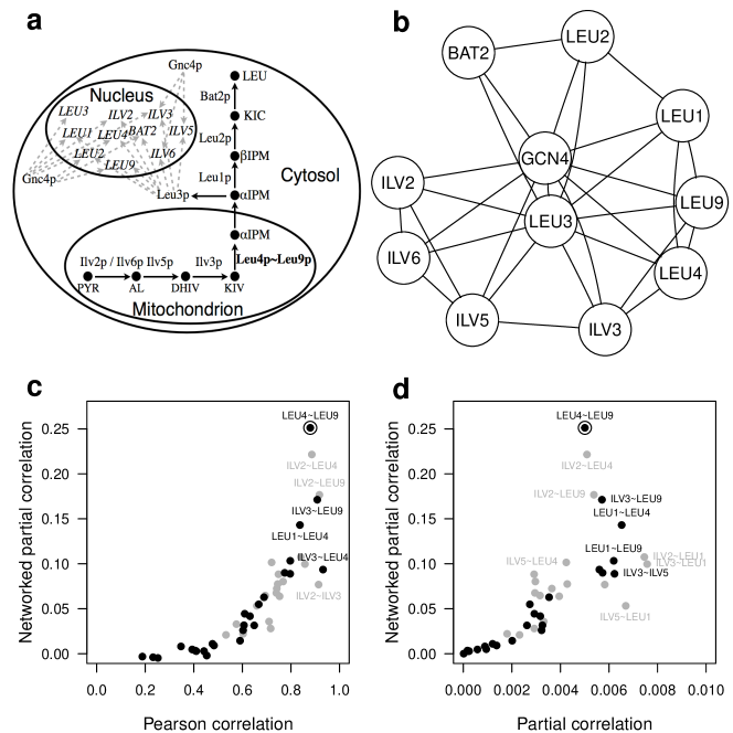
Figure 2: Analysis of the leucine biosynthesis pathway. (a) A schematic representation of the pathway (see Kohlhaw, 2003; Chin et al., 2008). Solid dots and arrows indicate metabolites and metabolic reactions. Dashed arrows indicate transcriptional regulatory associations. Metabolite abbreviations are placed next to the corresponding metabolite. Enzyme protein names are placed next to the corresponding metabolic reaction. Slash / and tilde $\sim$ symbols indicate protein complex and genetic interactions, respectively. (b) Undirected graph representing direct functional associations between genes involved in the pathway depicted in (a). (c) Networked partial correlation values on the $y$-axis as a function of Pearson correlation values on the $x$-axis. Black and grey dots correspond to present and missing edges in (b), respectively. A circle indicates the only known genetic interaction among genes in (b). (d) The same as (c) but the values on the $x$-axis are partial correlations.

We estimated partial correlation coefficients and their $p$-values for the null hypothesis of zero-partial correlation by using the empirical Bayes method of Schäfer and Strimmer (2005) that works by calculating a shrinkage estimate of the inverse covariance and is implemented in the R package GeneNet. To estimate vector correlations we exploited expression (5) and used the sparse canonical correlation analysis technique of Witten et al. (2009) implemented in the R package PMA. Full details on how the data analysis was conducted are available in the Supplementary Materials. Data and source code of the R scripts reproducing the results in this section are available at http://functionalgenomics.upf.edu/supplements/NPC4GI.

5.2 Analysis of the leucine biosynthesis pathway

The gene expression data by Brem and Kruglyak (2005) were generated by first crossing two different strains of yeast, one of them containing the deletion of the LEU2 gene that participates in the leucine biosynthesis pathway. Then, gene expression was profiled in the resulting collection of $n=112$ segregants. Because some of these offspring inherited the deletion of the LEU2 gene, these gene expression data show a large degree of variability of expression in genes involved in the leucine biosynthesis pathway, providing the opportunity to study gene expression changes associated with the activity of this pathway.

The leucine biosynthesis pathway, which is shown in Fig. 2(a), consists of a number of sequential reactions catalysed by different enzymes that allow yeast to convert pyruvate (PYR) into leucine (LEU). Among these reactions, a key role is played by a metabolic intermediate called $\alpha$-isopropylmalate ($\alpha$IPM), which binds to the homodimeric DNA binding protein Leu3p, which is a transcription factor regulating the expression of all the genes within the pathway. The transcriptional activity of all genes in the pathway, including LEU3 itself, is also regulated by the transcription factor Gcn4p. See (Kohlhaw, 2003; Chin et al., 2008) for a more comprehensive description of this pathway.

$\alpha$IPM is synthesised by either of the two enzymes encoded by the genes LEU4 and LEU9 (Kohlhaw, 2003), who are paralogues and form a duplicated gene pair that arose from the whole genome duplication of yeast. It is well known that the deletion of only one of these two genes is not sufficient to create a leucine-auxotrophic yeast mutant that would require a supply of leucine for growth (Kohlhaw, 2003). Consistent with this observation, the gene pair LEU4-LEU9 forms a genetic interaction whose double mutation produces a fitness defect that is more severe than what is expected from the combination of the single mutants (DeLuna et al., 2008). All other possible interactions between genes that are involved in the pathway (Fig. 2b) were either absent from the catalogue of quantitative genetic interaction profiles analysed in this paper (Costanzo et al., 2010) or did not have a negative and significant (false discovery rate (FDR) $<1$%) SGA interaction score.

One of the simpler buffering relationships behind a genetic interaction is the positive coexpression of two genes and, accordingly, we analysed only those pairs of genes in this pathway with positive Pearson, partial and networked partial, correlations, previously calculated from the expression data.

The comparison between these quantities shown in Figs. 2c and 2d reveals that the only known genetic interaction LEU4-LEU9 has the largest networked partial correlation among all the gene pairs, which is not so for Pearson or partial correlations. The following three gene pairs ranked by the networked partial correlation, ILV2-LEU4, ILV2-LEU9 and ILV3-LEU9, involve each of the two genes forming the known LEU4-LEU9 genetic interaction and the other intervening genes ILV2 and ILV3 are upstream of $\alpha$IPM, where they have more chance to affect its synthesis and, therefore, the entire operation of the pathway (Chin et al., 2008).

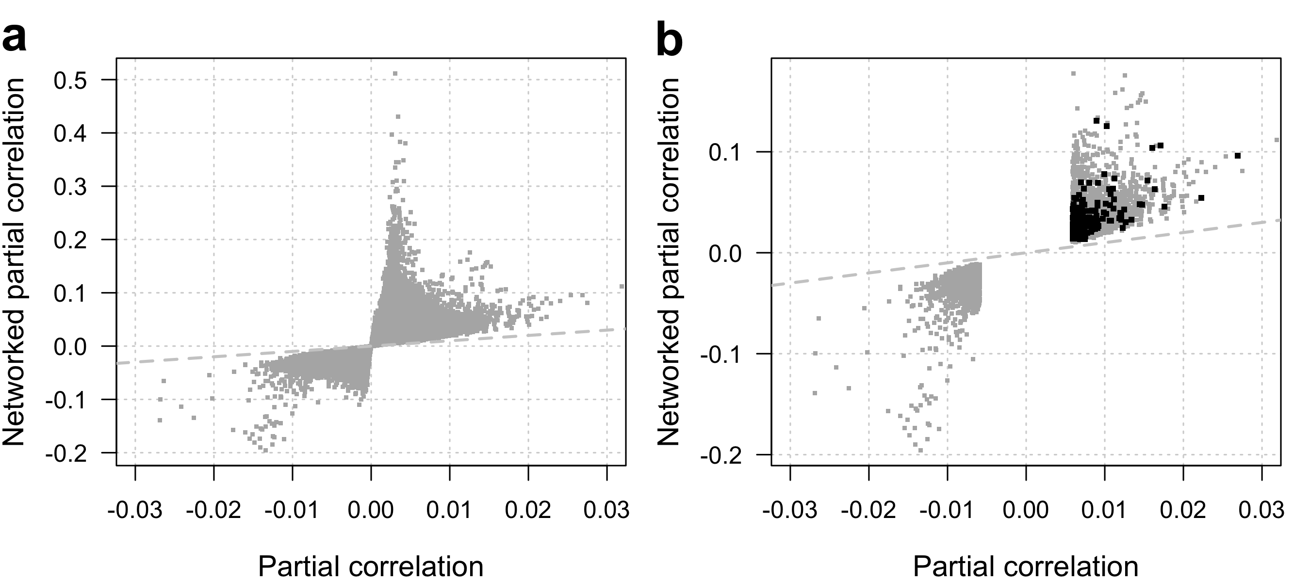
Figure 3: Networked partial correlations on the $y$-axis as a function of the corresponding partial correlations on the $x$-axis, calculated from yeast expression data (Brem and Kruglyak, 2005). (a) Values for all pairs of genes in the expression data set. (b) Values for those pairs with significant partial correlations (FDR $<1$%). Values for the filtered pairs shown in Figures 4 and 5 are highlighted in black. The grey dashed line indicates the axis where $x=y$ and is provided only as a visual guide.

5.3 Analysis of quantitative genetic interaction profiles

In this subsection we analyze the genomewide quantitative interaction profiles from Costanzo et al. (2010), defined by SGA scores and $p$-values associated with the profiled gene pairs. There were 4099 genes in common between the 4457 genes forming pairs with SGA scores and $p$-values, and the 6216 genes with expression data. We restricted the rest of the analysis to the 3,966,346 pairs formed by these 4099 genes. A comparison of the values of partial and networked partial, correlations, shown in Figure 3(a), reveals that differences between these two quantities grow proportionally to their absolute value. Note that small values of partial correlation may still become large networked partial correlation values.

Figure 4: SGA scores as function of the three different gene correlation measures. (a) SGA scores on the $y$-axis as function of Pearson correlations on the $x$-axis for gene pairs with largest Pearson correlation. There are as many pairs as gene pairs with significant partial correlation (FDR $<1$%). (b) The same as (a) but gene pairs were selected with significant partial correlation (FDR $<1$%). (c,d) SGA scores on the $y$-axis as function of partial and networked partial, correlations, respectively, on the $x$-axis. Gene pairs were selected as in (b).

Positive and negative SGA scores have a very different interpretation. While negative SGA scores indicate a fitness defect that is more severe than expected, positive ones identify double mutants whose fitness defect is less severe than expected (Costanzo et al., 2010). For this reason, and to provide a meaningful comparison between SGA scores and correlation measures, we restricted the subset of analyzed gene pairs as follows. First, we considered only 87,471 gene pairs with negative and significant SGA scores whose FDR $<1$% on the corrected SGA $p$-value. Second, we further restricted the analysis to gene pairs showing positive and significant coexpression.

When we considered Pearson correlation coefficients with a corrected $p$-value of FDR$<1$% to define such gene pairs, 6,889 of them were selected. The association between their SGA scores and their magnitude of the Pearson correlation was negligible possibly due to the large number of significant spurious associations (see Supplementary Materials). In contrast, when we considered significant partial correlation coefficients with FDR$<1$%, only 227 gene pairs were selected. To enable a more direct comparison of the performance of Pearson correlation coefficients we considered also selecting the top-227 gene pairs with largest positive Pearson correlation values. Selecting a top number of gene pairs with the largest marginal correlation, such as Pearson or Spearman, is a common strategy used in computational pipelines for selecting coexpressed genes potentially forming a genetic interaction (e.g., Jerby-Arnon et al., 2014).

Figure 5: SGA scores as function of different gene correlation measures, on a logarithmic scale. Panels (b), (c) and (d) show gene pairs with positive and significant partial correlation values at FDR$<1$%. Panel (a) shows the same number of gene pairs but selected with the largest positive Pearson correlation coefficient values.

The association of the largest values of Pearson correlation with SGA scores, remains non-significant, however, as shown in Fig. 4(a). This association is greatly improved by using Pearson correlation coefficients only on gene pairs whose partial correlation is significantly different from zero, as shown in Fig. 4(b). Yet, Figs. 4(c) and 4(d) show that the association with SGA scores can still improve when partial and networked partial correlations are used instead on those gene pairs.

Fig. 4 also shows that while larger coexpression values are associated with larger negative SGA scores, the trend is non-linear. Such a non-linearity probably arises from the restriction of SGA scores to negative values and gene coexpression to positive ones, so that a large fraction of pairs accumulate in values close to zero of both quantities.

To have a clearer picture of the differences between these three coexpression measures in relationship with SGA scores, we show in Fig. 5 the same values in logarithmic scale for absolute SGA scores, partial correlations and networked partial correlations. These plots reveal that there is a significant linear relationship between each of these three coexpression measures and SGA scores, albeit only when gene pairs are selected on the basis of a test for a zero-partial correlation coefficient; see Figs. 5(b), 5(c) and 5(d). However, among these significant associations, networked partial correlations explain a larger fraction of the variability of SGA scores ($R^{2}=0.16$) than Pearson ($R^{2}=0.09$) and partial correlations ($R^{2}=0.07$).

Figure 6: Regression of networked partial correlations on partial correlations, both on a logarithmic scale. (a) Scatter plot of both quantities with the regression line. (b) Scatter plot of the residuals of the regression as function of the fitted values.

We also investigated the extent to which networked partial correlations provide additional information over partial correlations. We first regressed networked partial correlations on partial correlations, obtaining a significant fit as expected (Fig. 6a). Then, we considered the following three linear models of the SGA scores: a first model where SGA scores are a linear function of partial correlation values only, a second model including the residuals of the former regression (Fig. 6b) as an additional term, and a third model as a linear function of the networked partial correlation values only.

	Model 1		Model 2		Model 3
(Intercept)	2.70	∗	2.70	∗	1.82
PAC	1.07	∗∗∗	1.07	∗∗∗	0.29
NPCresid			0.83	∗∗∗
NPC					0.83	∗∗∗
R2	0.07		0.16		0.16
RSS	213.57		193.94		193.94
$n=227$, Df $=1$, $F=22.67^{***}$
${}^{***}p<0.001$, ${}^{**}p<0.01$, ${}^{*}p<0.05$

Table 1: Comparison of three linear models of the SGA scores as function of the partial correlation (PAC) values only (model 1), of the PAC-values and the residuals of the networked partial correlation (NPC) values regressed on the PAC-values (model 2), and of the PAC-values and the NPC-values (model 3). The bottom line gives the sample size $n$, degrees of freedom (Df) and $F$-statistic for the analysis of variance of model 1 against model 2 and model 3. Both comparisons give exactly the same result.

The results, summarised in Table 1, show that the two models including networked partial correlations, or the residuals of their regression on partial correlations, provide a significantly better fit to SGA scores than the model that includes partial correlations alone ($p<0.001$).

6 Discussion

The theory that was developed by Jones and West (2005) associates a weight to every path of an undirected graph, and the simple observation that every edge of the graph is also a path allowed us to introduce the networking partial covariance, as a novel measure of association between pairs of variables. The theory of Section 4 shows that, in a context where the association structure between variables is represented by a network, the networked partial covariance can be regarded as a natural generalization of the covariance, thereby providing an additional motivation for its use.

The networked partial covariance can be normalized to obtain a networked partial correlation. We have shown that the latter has the form of an inflated version of the partial correlation and that it should be preferred to the partial correlation to address questions where the relevance the association between two variables also depends on the strength of the association of the corresponding edge with the rest of the network. This is so, for instance, for genetic interactions that confer robustness on cells in response to genetic perturbations. Our analysis of quantitative genetic interaction profiles in yeast highlights the relevance and usefulness of the networked partial correlation in this context.

Despite the improved performance of networked partial correlations, the fraction of variability they explain in quantitative genetic interaction profiles is rather modest ($R^{2}=0.16$). However, one should consider the fact that the identification of genetic interactions on the basis of gene expression data is a very challenging problem because, on the one hand, buffering relationships are only one of the many biological mechanisms affecting the expression levels of the genes. On the other hand, changes in gene expression may occur as a result of multiple types of effects other than genetic effecst, such as molecular, environmental and technical effects produced by the profiling instruments. For this reason, the prediction of genetic interactions is typically based on multiple biological features (Wong et al., 2004; Zhong and Sternberg, 2006; Conde-Pueyo et al., 2009; Deshpande et al., 2013; Jerby-Arnon et al., 2014), and the information provided by gene correlation measures is only one of the potential predictors. In this sense, the assessment of the improvement provided by the introduction of networked partial correlations within current computational pipelines for the prediction of genetic interactions is of potential interest.

We have estimated networked partial correlations by computing separately the partial correlation and the vector correlation by means of existing procedures developed to deal with the case $p\gg n$. More efficient estimates might be obtained by following a unitary approach to the estimate of this quantity, and future research should tackle this problem.

Appendix A Proofs

Proof of Theorem 3.1

If we set $P=\{x,y\}$ so that $|P|=2$ and $\bar{P}=V\backslash\{x,y\}$ then it follows from equation (1) that

$$\omega(\langle x,y\rangle{},\varSigma) = (-1)\;|\varSigma_{PP}|\;\kappa_{xy}$$ (12)

$$= (-1)\;|\varSigma_{PP\cdot\bar{P}}|\;\kappa_{xy}\;\frac{|\varSigma_{PP}|}{|\varSigma_{PP\cdot\bar{P}}|}$$

$$= \frac{-\kappa_{xy}}{|\mathit{K}_{PP}|}\;\frac{|\varSigma_{PP}|}{|\varSigma_{PP\cdot\bar{P}}|}$$

where in equation (12) we have used the fact that $\mathit{K}_{PP}=\varSigma_{PP\cdot\bar{P}}^{-1}$. We note that in equation (12) we have

$$\frac{-\kappa_{xy}}{|\mathit{K}_{PP}|}=\{\varSigma_{PP\cdot\bar{P}}\}_{xy}=\sigma_{xy\cdot V\backslash\{x,y\}},$$

and, furthermore, it follows from the definition of the vector alienation coefficient and equation (6) that

$$\frac{|\varSigma_{PP}|}{|\varSigma_{PP\cdot\bar{P}}|}=\left(\frac{|\varSigma_{P\cup\bar{P}P\cup\bar{P}}|}{|\varSigma_{PP}||\varSigma_{\bar{P}\bar{P}}|}\right)^{-1}=\frac{1}{\lambda_{(P)(\bar{P})}}=\frac{1}{1-\rho^{2}_{(P)(\bar{P})}}.$$

Hence, (12) can be written in the form

$$\omega(\langle x,y\rangle{},\varSigma)=\frac{\sigma_{xy.\bar{P}}}{1-\rho^{2}_{(P)(\bar{P})}},$$

as required.

Proof of Theorem 4.1

Let $A=V\backslash Q$. If $\mathit{K}$ implies the graph $\mathcal{G}=(V,\mathcal{E})$, then $\varSigma_{AA\cdot Q}^{-1}=\mathit{K}_{AA}$ implies the subgraph $\mathcal{G}_{A}=(A,\mathcal{E}_{A})$. Hence, if $\pi\in\Pi_{xy}$ is a path between $x$ and $y$ in $\mathcal{G}$ such that $V(\pi)\subseteq A$ then $\pi$ is also a path between $x$ and $y$ in $\mathcal{G}_{A}$ and it makes sense to compute the weight of $\pi$ with respect to the distribution of $X_{A}|X_{Q}$, that is $\omega(\pi,\varSigma_{AA\cdot Q})$. More specifically, it follows from equation (1) and (2) that

$$\omega(\pi,\varSigma_{V\backslash QV\backslash Q\cdot Q}) = (-1)^{|P|+1}\;|\varSigma_{PP\cdot Q}|\;\prod_{\{u,v\}\in\mathcal{E}(\pi)}\kappa_{uv}.$$

and an immediate consequence of Theorem 2.1 is that

$$\sigma_{xy\cdot Q} = \sum_{\pi\in\Pi_{xy};V(\pi)\subseteq A}\omega(\pi,\varSigma_{AA\cdot Q})$$ (13)

where, for $\pi\in\Pi_{xy}$ with $V(\pi)\subseteq A$,

$$\omega(\pi,\varSigma_{AA\cdot Q}) = (-1)^{|P|+1}\;|\varSigma_{PP\cdot Q}|\;\prod_{\{i,j\}\in\mathcal{E}(\pi)}\kappa_{ij}.$$

If we divide both sides of equation (13) by

$$1-\rho^{2}_{(xy)(Q)}=\frac{|\varSigma_{QQ\cdot\{x,y\}}|}{|\varSigma_{QQ}|},$$

then we obtain

$$\omega_{xy\cdot(Q)} = \sum_{\pi\in\Pi_{xy};V(\pi)\subseteq A}\omega(\pi,\varSigma_{AA\cdot Q})\frac{|\varSigma_{QQ}|}{|\varSigma_{QQ\cdot\{x,y\}}|},$$

where

$$\omega(\pi,\varSigma_{AA\cdot Q})\frac{|\varSigma_{QQ}|}{|\varSigma_{QQ\cdot\{x,y\}}|} = (-1)^{|P|+1}\;\frac{|\varSigma_{PP\cdot Q}||\varSigma_{QQ}|}{|\varSigma_{QQ\cdot\{x,y\}}|}\;\prod_{\{i,j\}\in\mathcal{E}(\pi)}\kappa_{ij}$$

$$= (-1)^{|P|+1}\;\frac{|\varSigma_{QQ\cdot P}||\varSigma_{PP}|}{|\varSigma_{QQ\cdot\{x,y\}}|}\;\prod_{\{i,j\}\in\mathcal{E}(\pi)}\kappa_{ij}$$

$$= \omega(\pi,\varSigma)\times\frac{|\varSigma_{QQ\cdot P}|}{|\varSigma_{QQ\cdot\{x,y\}}|}$$

$$= \omega(\pi,\varSigma)\times(1-\rho^{2}_{(P\backslash\{x,y\})(Q)\cdot\{x,y\}}),$$

as required.

Appendix B Limited-order networked partial covariance decomposition on four vertices

For the graph in Fig. 7 we focus on the decomposition of the covariance $\sigma_{12}$, i.e. on all the paths between vertices $1$ and $2$.

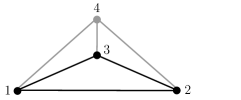
Figure 7: Complete graph on four vertices: the grey part highlights the connection of vertex 4 with the rest of the graph.

It follows from Theorem 2.1 that $\sigma_{12}$ can be computed as the sum of the five path weights that are given in Table 2, where we use the suppressed notation $\varSigma_{12}$ to denote $\varSigma_{\{1,2\}\{1,2\}}$. We remark that this example also covers the case where the graph is not complete because it is sufficient to recall that the corresponding entry of the concentration matrix is equal to 0 and, consequently, the same is true for every path involving such edges.

Table 2: Weights of the paths between vertices $1$ and $2$ in the graph of Fig. 7

Path	Path weight
$1-\!\!\!-{}\ 2$	$\omega_{12\cdot(34)}$	$=$	$-\kappa_{12}$ $|\varSigma_{12}|$
$1-\!\!\!-{}\ 3-\!\!\!-{}\ 2$	$\omega(\langle 1,3,2\rangle,\varSigma)$	$=$	$+\kappa_{13}\;\kappa_{32}$ $|\varSigma_{123}|$
$1-\!\!\!-{}\ 4-\!\!\!-{}\ 3-\!\!\!-{}\ 2$	$\omega(\langle 1,4,3,2\rangle,\varSigma)$	$=$	$-\kappa_{14}\;\kappa_{43}\;\kappa_{32}$ $|\varSigma|$
$1-\!\!\!-{}\ 3-\!\!\!-{}\ 4-\!\!\!-{}\ 2$	$\omega(\langle 1,3,4,2\rangle,\varSigma)$	$=$	$-\kappa_{13}\;\kappa_{34}\;\kappa_{42}$ $|\varSigma|$
$1-\!\!\!-{}\ 4-\!\!\!-{}\ 2$	$\omega(\langle 1,4,2\rangle,\varSigma)$	$=$	$+\kappa_{14}\;\kappa_{42}$ $|\varSigma_{124}|$

Consider now the case where we marginalize over $X_{4}$ so that $Q=\{3\}$. If we write $\varSigma^{-1}_{Q\cup\{x,y\}Q\cup\{x,y\}}=\varSigma_{123}^{-1}=\{\kappa^{*}_{ij}\}_{i,j\in\{1,2,3\}}$, then the weights associated with the paths between $1$ and $2$ in the subgraph of the graph in Fig. 7 induced by $\{1,2,3\}$ are given in Table 3.

Table 3: Weights of the paths between vertices $1$ and $2$ in the subgraph of the graph in Fig. 7 induced by $\{1,2,3\}$, after marginalization over variable $X_{4}$.

Path	Path weight
$1-\!\!\!-{}\ 2$	$\omega_{12\cdot(3)}$	$=$	$-\kappa^{*}_{12}$ $|\varSigma_{12}|$
$1-\!\!\!-{}\ 3-\!\!\!-{}\ 2$	$\omega(\langle 1,3,2\rangle,\varSigma_{123})$	$=$	$+\kappa^{*}_{13}\;\kappa^{*}_{32}$ $|\varSigma_{123}|$

It follows from Theorem 4.1 that

$$\omega_{12\cdot(3)} = \omega_{12\cdot(3)}$$

$$+ \omega(\langle 1,4,2\rangle,\varSigma)\times(1-\rho^{2}_{34\cdot 12})$$

If we exploit the fact that the sum of the five path weights in Table 2 is equal to the sum of the two path weights in Table 3, i.e. equal to $\sigma_{12}$, then we can decompose the weight of the path $\langle 1,3,2\rangle$, relative to $\mathbf{X}_{\{1,2,3\}}$, as follows

$$\omega(\langle 1,3,2\rangle,\varSigma_{123}) = \omega(\langle 1,3,2\rangle,\varSigma)$$

$$+ \omega(\langle 1,4,3,2\rangle,\varSigma)$$

$$+ \omega(\langle 1,3,4,2\rangle,\varSigma)$$

$$+ \omega(\langle 1,4,2\rangle,\varSigma)\times\rho^{2}_{34\cdot 12}.$$

We can conclude that the weight, relative to $\mathbf{X}_{\{1,2,3\}}$, of the path $\langle 1,2\rangle$ can be obtained by adding to the weight, relative to $\mathbf{X}_{\{1,2,3,4\}}$, of the path $\langle 1,2\rangle$ the proportion $(1-\rho^{2}_{34\cdot 12})$ of the weight of path $\langle 1,4,2\rangle$; note that $(1-\rho^{2}_{(34)(12)})=1$ if the edge $\{3,4\}$ does not belong to the graph. In addition, the weight, relative to $\mathbf{X}_{\{1,2,3\}}$, of the path $\langle 1,3,2\rangle$ can be be obtained by adding to the weight, relative to $\mathbf{X}_{\{1,2,3,4\}}$, of the path $\langle 1,3,2\rangle$ the proportion $\rho^{2}_{34\cdot 12}$ of the weight of path $\langle 1,4,2\rangle$, with $\rho^{2}_{(34)(12)}=0$ if $\{3,4\}$ does not belong to the graph, and, furthermore, the weights of all the remaining paths between $1$ and $2$ in the graph which involve the vertex 3.

References

- Baryshnikova et al. (2010) Baryshnikova, A., M. Costanzo, Y. Kim, H. Ding, J. Koh, K. Toufighi, J.-Y. Youn, J. Ou, B.-J. San Luis, S. Bandyopadhyay, et al. (2010). Quantitative analysis of fitness and genetic interactions in yeast on a genome scale. Nat. Methods 7(12), 1017–1024.
- Brem and Kruglyak (2005) Brem, R. B. and L. Kruglyak (2005). The landscape of genetic complexity across 5,700 gene expression traits in yeast. Proc. Natl. Acad. Sci. U.S.A. 102(5), 1572–1577.
- Castelo and Roverato (2006) Castelo, R. and A. Roverato (2006). A robust procedure for Gaussian graphical model search from microarray data with larger than . J. Mach. Learn. Res. 7, 2621–2650.
- Chen and Pearl (2015) Chen, B. and J. Pearl (2015). Graphical tools for linear structural equation modeling. Technical Report R-432, Cognitive Systems Laborary, University of California at Los Angeles, Los Angeles, CA, USA.
- Chin et al. (2008) Chin, C.-S., V. Chubukov, E. R. Jolly, J. DeRisi, and H. Li (2008). Dynamics and design principles of a basic regulatory architecture controlling metabolic pathways. PLoS Biol 6(6), e146.
- Conde-Pueyo et al. (2009) Conde-Pueyo, N., A. Munteanu, R. V. Solé, and C. Rodríguez-Caso (2009). Human synthetic lethal inference as potential anti-cancer target gene detection. BMC Sys. Biol. 3(1), 116.
- Costanzo et al. (2010) Costanzo, M., A. Baryshnikova, J. Bellay, Y. Kim, E. D. Spear, C. S. Sevier, H. Ding, J. L. Koh, K. Toufighi, S. Mostafavi, et al. (2010). The genetic landscape of a cell. Science 327(5964), 425–431.
- Cox and Wermuth (1996) Cox, D. R. and N. Wermuth (1996). Multivariate Dependencies: Models, analysis and interpretation. Chapman and Hall, London.
- De La Fuente et al. (2004) De La Fuente, A., N. Bing, I. Hoeschele, and P. Mendes (2004). Discovery of meaningful associations in genomic data using partial correlation coefficients. Bioinformatics 20(18), 3565–3574.
- DeLuna et al. (2008) DeLuna, A., K. Vetsigian, N. Shoresh, M. Hegreness, M. Colón-González, S. Chao, and R. Kishony (2008). Exposing the fitness contribution of duplicated genes. Nature genetics 40(5), 676–681.
- Dempster (1972) Dempster, A. P. (1972). Covariance selection. Biometrics 28(1), 157–175.
- Deshpande et al. (2013) Deshpande, R., M. K. Asiedu, M. Klebig, S. Sutor, E. Kuzmin, J. Nelson, J. Piotrowski, S. H. Shin, M. Yoshida, M. Costanzo, et al. (2013). A comparative genomic approach for identifying synthetic lethal interactions in human cancer. Cancer Res. 73(20), 6128–6136.
- Eddy (2006) Eddy, S. R. (2006). Total information awareness for worm genetics. Science 311, 1381–1382.
- Eisen et al. (1998) Eisen, M. B., P. T. Spellman, P. O. Brown, and D. Botstein (1998). Cluster analysis and display of genome-wide expression patterns. Proc. Natl. Acad. Sci. U.S.A. 95(25), 14863–14868.
- Friedman (2004) Friedman, N. (2004). Inferring cellular networks using probabilistic graphical models. Science 303(5659), 799–805.
- Hotelling (1936) Hotelling, H. (1936). Relations between two sets of variates. Biometrika 28(3/4), 321–377.
- Jerby-Arnon et al. (2014) Jerby-Arnon, L., N. Pfetzer, Y. Y. Waldman, L. McGarry, D. James, E. Shanks, B. Seashore-Ludlow, A. Weinstock, T. Geiger, P. A. Clemons, et al. (2014). Predicting cancer-specific vulnerability via data-driven detection of synthetic lethality. Cell 158(5), 1199–1209.
- Jones and West (2005) Jones, B. and M. West (2005). Covariance decomposition in undirected Gaussian graphical models. Biometrika 92(4), 779–786.
- Kim and Timm (2006) Kim, K. and N. Timm (2006). Univariate and Multivariate General Linear Models: Theory and applications with SAS. CRC Press.
- Kohlhaw (2003) Kohlhaw, G. B. (2003). Leucine biosynthesis in fungi: entering metabolism through the back door. Microbiology and Molecular Biology Reviews 67(1), 1–15.
- Lauritzen (1996) Lauritzen, S. L. (1996). Graphical Models. Oxford University Press.
- Luo et al. (2009) Luo, J., M. J. Emanuele, D. Li, C. J. Creighton, M. R. Schlabach, T. F. Westbrook, K.-K. Wong, and S. J. Elledge (2009). A genome-wide RNAi screen identifies multiple synthetic lethal interactions with the Ras oncogene. Cell 137(5), 835–848.
- Malioutov et al. (2006) Malioutov, D. M., J. K. Johnson, and A. S. Willsky (2006). Walk-sums and belief propagation in Gaussian graphical models. J. Mach. Learn. Res. 7, 2031–2064.
- Mardia et al. (1979) Mardia, K. V., J. T. Kent, and J. M. Bibby (1979). Multivariate Analysis. London: Academic Press.
- Nijman (2011) Nijman, S. M. (2011). Synthetic lethality: general principles, utility and detection using genetic screens in human cells. FEBS Lett. 585(1), 1–6.
- Robert and Escoufier (1976) Robert, P. and Y. Escoufier (1976). A unifying tool for linear multivariate statistical methods: the RV-coefficient. Applied statistics 25(3), 257–265.
- Rozeboom (1965) Rozeboom, W. W. (1965). Linear correlations between sets of variables. Psychometrika 30(1), 57–71.
- Schäfer and Strimmer (2005) Schäfer, J. and K. Strimmer (2005). An empirical Bayes approach to inferring large-scale gene association networks. Bioinformatics 21(6), 754–764.
- Timm (2002) Timm, N. H. (2002). Applied Multivariate Analysis. Springer-Verlag, New York.
- Tucker and Fields (2003) Tucker, C. L. and S. Fields (2003). Lethal combinations. Nature Genet. 35(3), 204–205.
- Tur et al. (2014) Tur, I., A. Roverato, and R. Castelo (2014). Mapping eQTL networks with mixed graphical Markov models. Genetics 198(4), 1377–1393.
- Whittaker (1990) Whittaker, J. (1990). Graphical Models in Applied Multivariate Analysis. John Wiley & Sons, Chichester.
- Winzeler et al. (1999) Winzeler, E. A., D. D. Shoemaker, A. Astromoff, H. Liang, K. Anderson, B. Andre, R. Bangham, R. Benito, J. D. Boeke, H. Bussey, et al. (1999). Functional characterization of the S. cerevisiae genome by gene deletion and parallel analysis. Science 285(5429), 901–906.
- Witten et al. (2009) Witten, D. M., R. Tibshirani, and T. Hastie (2009). A penalized matrix decomposition, with applications to sparse principal components and canonical correlation analysis. Biostatistics 10(5), 515–534.
- Wong et al. (2004) Wong, S. L., L. V. Zhang, A. H. Tong, Z. Li, D. S. Goldberg, O. D. King, G. Lesage, M. Vidal, B. Andrews, H. Bussey, et al. (2004). Combining biological networks to predict genetic interactions. Proc. Natl. Acad. Sci. U.S.A. 101(44), 15682–15687.
- Wright (1921) Wright, S. (1921). Correlation and causation. J. Agric. Res. 20(7), 557–585.
- Zhong and Sternberg (2006) Zhong, W. and P. W. Sternberg (2006). Genome-wide prediction of C. elegans genetic interactions. Science 311(5766), 1481–1484.
- Zuo et al. (2014) Zuo, Y., G. Yu, M. G. Tadesse, and H. W. Ressom (2014). Biological network inference using low order partial correlation. Methods 69(3), 266–273.