Statistical Analysis of Persistence Intensity Functions
Yen-Chi Chen Daren Wang Alessandro Rinaldo Larry Wasserman
Carnegie Mellon University Department of Statistics
Abstract
Persistence diagrams are two-dimensional plots that summarize the topological features of functions and are an important part of topological data analysis. A problem that has received much attention is how deal with sets of persistence diagrams. How do we summarize them, average them or cluster them? One approach — the persistence intensity function — was introduced informally by Edelsbrunner, Ivanov, and Karasev (2012). Here we provide a modification and formalization of this approach. Using the persistence intensity function, we can visualize multiple diagrams, perform clustering and conduct two-sample tests.
1 Introduction
Topological data analysis (TDA) is an emerging area in statistics and machine learning [2, 14]. The goal of TDA is to extract useful topological information from a given data and make inferences using these information. TDA has been applied various fields such as pattern recognition [8], computer vision [15], and biology [23, 22].
One of the most popular and powerful approaches to TDA is persistent homology. This is a multiscale approach that finds topological features at various scales. The result is summarized in a two dimensional plot called a persistence diagram [9, 11, 14, 13, 31]. Given a data set with , we first find a summary function . Examples include the distance function or the kernel density estimator where is a kernel and is a bandwidth. The persistence diagram summarizes the topological information of the level sets of and converts it into points that can be represented by a 2-D diagram . For distance functions, one uses the lower level sets. For density estimator, one uses the upper level sets. The function is a random function. Hence, the corresponding persistence diagram is also random.
Now suppose we have datasets giving rise to summary functions which in turn give rise to diagrams . The following question now arises: how do we summarize the diagrams? For example how do we average the diagrams or cluster the diagrams? One approach is based on the notion of Frechet means [18, 27]. Here, the space of all persistence diagrams is endowed with a metric (called the bottleneck distance). The space is very complicated and the Frechet mean is a way to define averages in this space. This method is mathematically rigorous but is very complex is not easy for the user to understand.
The second method is based on converting the diagram into a set of one dimensional functions called landscapes [1]. The statistical properties of landscapes were further investigated in [6, 7, 14].
The landscape approach is quite simple but the results can be hard to interpret. Perhaps the most appealing method is due to [12]. They introduce the intensity function which is very easy to interpret. They divide the plane into cells, the count the number of points in each cell. This converts the persistence diagram into a two-dimensional histogram. The resulting function is easy to visualize, and can be averaged and clustered very easily. Similar ideas were introduced by [25, 8, 24].
The purpose of this paper is to make the intensity function approach more rigorous. We also modify the approach: instead of using histograms (cell counts) we use kernel smoothing which leads to much smoother summaries.
The diagrams now give rise to two-dimensional intensity functions . Mathematically, we regard these as random functions drawn from some measure . The mean gives a well-defined population quantity. We then show that we can visualize the relative proximity of diagrams and perform clustering for diagrams and conduct a two sample test for two sets of diagrams.

2 The Persistence Intensity Function
We begin with a short introduction to the persistent homology [13, 31]. Given a function , let the upper level set be . changes as the level varies. Persistent homology studies how the topological features of change when the level changes. Some common topological features include connected components (the zeroth order homology), loops (the first order homology), voids (the second order homology), etc. For more detailed discussion and definitions for the persistence homology, we refer to [11].
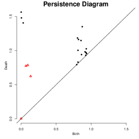
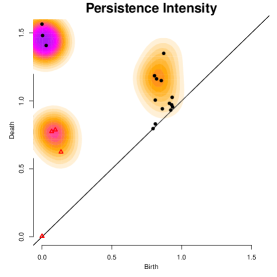
When the level varies, new topological features may be created (birth) and some existing features may be eliminated (death). The persistence diagram is a diagram that keep track of the birth and the death of each topological features. See the left and middle panel of Figure 1 for an example of persistence diagram generated from a function. Formally, the pth persistence diagram is the collection of points in the extended plane , where such that each point in the diagram represents a distinct -th order topological feature that are created when and is destroyed when . Thus, each persistence diagram can be presented as a collection of points such that each denotes the birth time and death time of -th feature.
Remark: One usually defines persistent homology in terms of lower level sets. But for probability density functions, upper level sets are of more interest. The result is that the points will appear below the diagonal on the diagram. However, is it customary to put the points above the diagonal. Thus we simply switch the birth and death times which gives the usual diagram although, techincally, we have births coming after deaths. Moreover, we ignore the zeroth order topological feature with longest life time since this feature represents the entire space; it has infinite lifetime and contains no useful information.
Given a (random) function generated from a dataset that is sampled from a distribution , its persistence diagram
is a random object. The random function is typically generated from density estimates, or the distance function [14] or something called the distance to a measure [5, 4] of .
Our first step is to convert the persistence diagram into a measure. We define a random measure using as , where is a point mass at and is a weight. In this paper, we take the weight to be . This places less weight to features near the diagonal which are features with very short lifetimes. Other weights can be used as well. Now, is a random measure in such that the point mass located at has weight which equals its lifetime.
For each Borel set of , the persistence intensity measure is defined as
where the expectation is with respect to . The persistence intensity function (or persistence intensity)
| (1) |
where is a ball center at with radius . The persistence intensity at position is a weighted intensity for the presence of a topological at the given location. The persistence intensity function is the parameter of interest to us. Note that the persistence intensity is zero below the diagonal, so smoothing estimators would suffer from boundary bias (see, e.g., page 73 of [29]) along the diagonal. By adding the weight that is proportional to the life time, we can alleviate this issue since points around diagonal (boundary) are given a very low weight.
However, in practice we do not know so that has to be estimated. Given a diagram , we estimate the intensity by
where the sum is over all features, is a symmetric kernel function such as a Gaussian and is the smoothing parameter. In other words, is just the smoothed version of the persistence measure . Figure 1 presents an example for a single diagram.
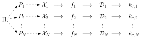
Now we consider the case that we have multiple datasets . The data in data set come from a distribution . The distributions are themselves random draws from some distribution which we denote by . Namely, we use to generate , and sample from to obtain , and finally use to construct . In this case, are iid random functions from some measure . Figure 2 shows a diagram for how these quantities are generated from one another. Note that there are two sources of randomness: and each . It is easy to see that if is given, the randomness of , the persistence diagram , and its associated random measure are determined by . For each distribution , we have a persistence intensity by equation (1)
and using the given diagram , we have an estimator
Note that depends on so it is actually a random quantity. However, we cannot consistently estimate each individual since we only have one diagram. On the other hand, if we consider the population version of intensity function, we can consistently estimate it.
There are two ways to define a population intensity function and later we will show that they are the equivalent. For the first definition, we define
Namely, is the average intensity using the distribution . Alternatively, we consider the distribution , which is the ‘mean’ distribution of . Let be a sample from . Then we define
by equation (1). Both and are population level quantity. The following lemma shows that they are the same.
Lemma 1
Let be defined as the above. Assume are bounded. Then
We always assume both are bounded so they are the same. For simplicity we write
| (2) |
A nonparametric estimator for the population intensity function is
| (3) |
Essentially, this is the sample average for the intensity function.
One may consider other weights such as
where is the dimension of -th topological feature and is some smooth function with . The reason we impose the constraint is to avoid a discontinuity of along the diagonal since we will not have any topological features below the diagonal line. The function determines how we want to give different weights to topological features with different dimensions and each is a function that determines how we want to give weight to the dimensional topological features according to their lifetime. Note that the parameter of interest depends on the weight we choose. In this paper, we use life time as the weight , which is the case that and . Although our theoretical analysis is done for the this simple case, it can be generalized to other weights easily.
3 Statistical Analysis
Here we study the asymptotic behavior of . Throughout this paper, we assume all random functions are Morse functions [19, 20, 21]. This means that the Hessian is non-degenerate at its critical points [9, 7, 5].
For a univariate function , let denote its -th derivative. We make the following assumptions.
-
(A1)
The persistence intensity function and has at least two bounded continuous derivatives.
-
(A2)
and .
-
(K)
The kernel function is symmetric, at least bounded twice continuously differentiable. Moreover, .
(A1) requires the persistence intensity to be well defined and smooth. Assumption (A2) is to regularize the integrated behavior for and its derivatives. Assumption (K) is a common assumption for kernel smoothing method such as the kernel density estimation and kernel regression [29, 26].
A direct result from assumption (A1) is the following useful lemma.
Lemma 2
Assume (A1) for and consider the case where the sample is from . Then for any twice differentiable function ,
| (4) | ||||
Lemma 4 shows that the expectation of integration (first expression) is equivalent to integration of expectation (last expression).
The next result, which is based on Lemma 4, controls the bias for the smoothed persistence intensity estimator.
Lemma 3
Assume (A1) for and assume (K) and consider the case where the sample is from . Then the bias for estimating using a single smoothed function is
for some constant that depends only on the kernel function .
This bias is essentially the same as the bias for nonparametric density estimation; see, e.g., page 133 of [29]. Lemma 3 shows that the bias is small for a small , and the variance of is of the order of .
Now we prove that the sample average estimator is a consistent estimator of the population under the mean integrated square error (MISE) [26].
Theorem 4
Assume (A1–2) and (K). Then mean integrated square error for
which implies the optimal smoothing bandwidth
Theorem 4 gives the mean integrated square error rate for the estimator and also the optimal rate of smoothing parameter when we have more and more diagrams. An interesting feature for Theorem 4 is that this rate is the same as the kernel density estimator in dimension [29]. This is reasonable since the smoothed intensity function is to smooth a measure in 2-D. Note that assumptions (A1) and (K) together are enough for the consistency for the (pointwise) mean square error and the rate is at the same order of MISE.
Before we end this section, we show the asymptotic normality of .
Theorem 5
Assume (A1–2) and (K). Then
where denotes the convergence in distribution and is some function depending only on and the kernel function .
The proof to this theorem is simply an application of the central limit theorem so we omit it.
4 Applications of Intensity Functions
The power of the persistence intensity function is that the smoothing technique converts a persistence diagram into a smooth function that carries topological information of the original function. Thus, we can apply methods for comparing functions to analyze the similarity between diagrams.
4.1 Clustering and Visualization
[3] used persistent homology to cluster images. They computed the bottleneck distance between each pair of diagrams and mapped the points to the plane using multidimensional scaling (MDS) [17] to visualize the results. Here we consider the same idea using persistence intensity functions.
For pairs of diagrams, say and , we first compute their smoothed persistence intensity and and then calculate their pairwise difference using some loss functions such as loss. Namely,
This allows us to construct a pair distance matrix for diagrams . Each element denotes the distance between diagram and diagram . Given , we can use techniques from MDS to visualize several diagrams. This visualization shows the relative proximity among diagrams in terms of the persistence intensity.
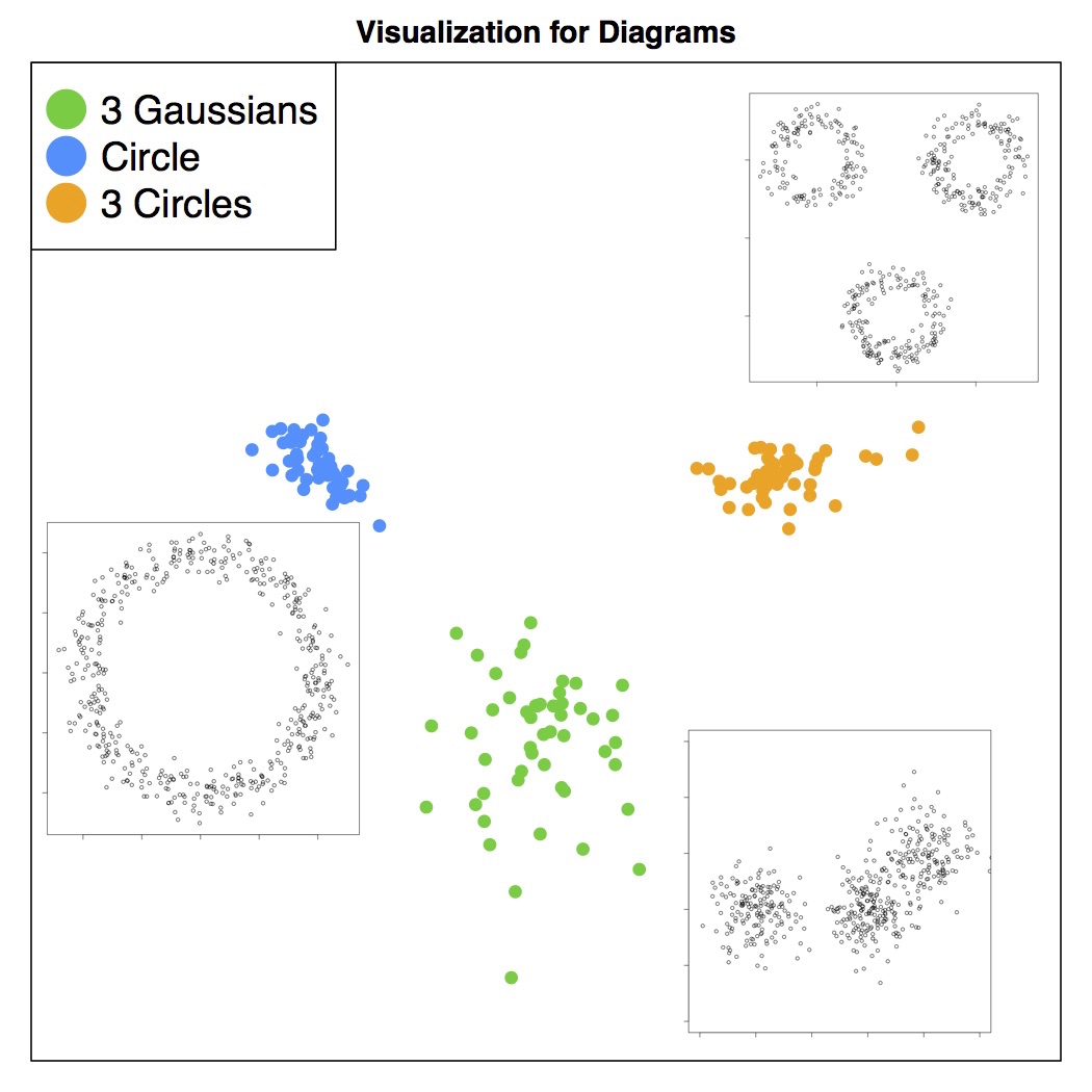
Figure 3 presents an example for using persistence intensity to visualize diagrams generated from three different populations. The three populations are the kernel density estimates of three types of point clouds: one circle, three circles, and three Gaussian mixtures. One circle is a uniform distribution with radius and corrupted with a Gaussian noise with standard deviation . Three circles is a uniform random distribution around three circles centered at , , and with radius and then we add Gaussian noise with standard deviation . The three Gaussian mixture is three Gaussians centered at , , and with standard deviation along both axes and zero correlation. We generate the point cloud with size points and then use kernel density estimator with Gaussian kernel and smoothing parameter . Thus, each random function is an estimated density function for a point cloud. For each of the three types of data, we generate 50 point clouds, so we have random functions (density estimates). We then compute the persistence diagrams for the random functions and smooth the diagrams, using , into intensity functions. Given the intensity functions, we use distance to construct the pairwise distance matrix and then use classical multidimensional scaling (MDS) [17] to visualize the data.
Moreover, we can use the idea of spectral clustering [28] to cluster and visualize these diagrams simultaneously. Figure 4 presents an example for the dataset from the Stanford 3D Scanning Repository [10]. The dataset is a point cloud characterizing the 3D surfaces of objects at different angles when taking 3D scanning. Thus, each object has several point clouds and each point cloud represent the 3D image of this object at one particular angle. We use the bunny, the dragon, the happy Buddha, and three different focuses of the Armadillo. For each point cloud, we use distance function and compute its persistence diagrams. Then we smooth the persistence diagrams using and impose times weight for the first order homology features (loops) to get the smoothed persistence estimator. We use distance to compare pairwise distance and then convert the distance matrix into a similarity matrix by . Finally we perform normalize cut spectral clustering over the similarity matrix . We use the two eigenvectors (correspond to the two smallest eigenvalues) to visualize and cluster data points. The visualization is given on the top panel of Figure 4. It shows a clear pattern that Armadillos (purple) aggregate at the left part; the bunny (green) and the dragon (blue) are at the center of the figure; the happy Buddha (orange) is on the right side. We then perform k-means clustering [16] with to the first two eigenvectors. The three red crosses denote the cluster center and the two straight lines are the boundaries of clusters. We give the confusion matrix at the bottom panel. It shows that the first cluster contains majority of Armadillos; the second cluster belongs to bunny and dragon; the third cluster is dominated by Happy Buddha.
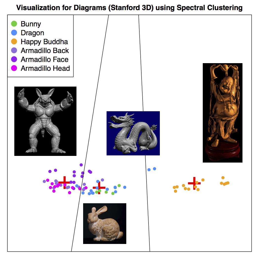
| 1 | 2 | 3 | |
|---|---|---|---|
| Armadillo Back | 9 | 3 | 0 |
| Armadillo Face | 10 | 2 | 0 |
| Armadillo Head | 11 | 1 | 0 |
| Bunny | 0 | 6 | 0 |
| Dragon | 1 | 12 | 2 |
| Happy Buddha | 0 | 0 | 15 |
4.2 Persistence Two Sample Tests
Assume that we are given two sets of diagrams, denoted as
The goal is to determine if these two sets of diagrams are generated from the same population or not.
A testing procedure based on the persistence intensity function is as follows. Let and be the persistence intensity for the two populations. Then the null hypothesis is
Based on intensity estimators from both populations, there are many ways to carry out the test. Let be the intensity estimator based on data from first population and be the intensity estimator from second population. One example for carrying the test is to use the distance
as a test statistics and then perform permutation test (see, e.g., section 10.5 of [30]) to get the p-value or bootstrap the test statistics to get the variance and convert it into z-score.
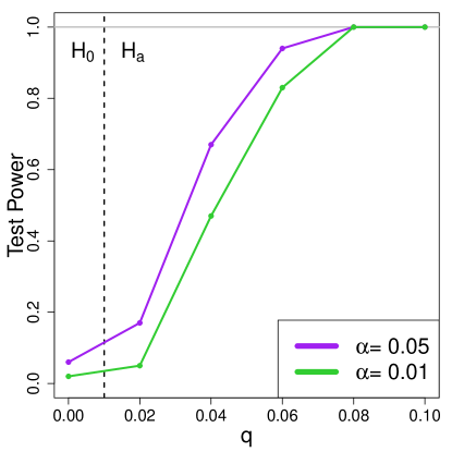
Figure 5 presents an example for the two sample test. We consider point clouds from two distributions:
where is the uniform distribution over a circle with unit radius. Namely, is just uniform distribution over the rectangle and is the same as with probability and with probability it generates a random point on a unit circle. We consider . Note that when , the two distributions are the same so that the power of the test should be the same as its significance level. We generate points for each point cloud and generate number of point clouds for each distribution. Then we apply kernel density estimator for each point cloud with smoothing parameter to obtain persistence diagrams. Finally, we use to smooth the diagram into persistence intensities and compute the average persistence intensity for both sample and then apply distance with times permutation test to compute the p-values. We consider two significance levels (purple) and (green). In Figure 5, the test at both significance level controls type-I error ( case). Moreover, the power for the test converges to rapidly even when two distributions are just slightly different ( indicates that only less than roughly of the data points in each point cloud are from different distributions).
5 Conclusion
In this paper, we study the persistence intensity as a summary for topological features over distribution of random functions. We propose a smoothed estimator for the intensity function and derive statistical consistence for this smoothed estimator. The main idea is to smooth persistence diagrams into functions. This smoothing technique also allows us to visualize persistence diagrams, perform clustering and conduct two-sample tests. Our examples suggest that the intensity function contains useful topological information.
Appendix A Proofs
Proof.[Proof for Lemma 1] Since , by dominated convergence theorem
Proof.[Proof for Lemma 4]
Note that can be written as
where Thus, by moving into the expectation,
Since is bounded, by dominated convergence theorem and Fubini’s theorem, we can exchange the limit, expectation, and integrations,
Note that we have
by using the change of variable . Plugging this into the previous equality proves the result.
Proof.[Proof for Lemma 3]
By definition
Now apply Lemma 4 with
we obtain
where is some constant. Note that we use Talyor expansion to the Hessian in the last equality and the first derivatives integrated to since the kernel function is symmetric.
Proof.[Proof for Theorem 4]
The mean integrated errors can be factorized into the following two terms
where
Since and the bias
by Lemma 3. The variance follows from standard calculation of nonparametric estimation that
Therefore, the mean integrated square error is at rate . By equating the two rates, we obtain the optimal smoothing parameter .
References
- [1] Peter Bubenik, Statistical topological data analysis using persistence landscapes, arXiv preprint arXiv:1207.6437 (2012).
- [2] Gunnar Carlsson, Topology and data, Bulletin of the American Mathematical Society 46 (2009), no. 2, 255–308.
- [3] Frédéric Chazal, David Cohen-Steiner, Leonidas J Guibas, Facundo Mémoli, and Steve Y Oudot, Gromov-hausdorff stable signatures for shapes using persistence, Computer Graphics Forum, vol. 28, Wiley Online Library, 2009, pp. 1393–1403.
- [4] Frédéric Chazal, David Cohen-Steiner, and Quentin Mérigot, Geometric inference for probability measures, Foundations of Computational Mathematics 11 (2011), no. 6, 733–751.
- [5] Frédéric Chazal, Brittany T Fasy, Fabrizio Lecci, Bertrand Michel, Alessandro Rinaldo, and Larry Wasserman, Robust topological inference: Distance to a measure and kernel distance, arXiv preprint arXiv:1412.7197 (2014).
- [6] Frédéric Chazal, Brittany Terese Fasy, Fabrizio Lecci, Alessandro Rinaldo, Aarti Singh, and Larry Wasserman, On the bootstrap for persistence diagrams and landscapes, arXiv preprint arXiv:1311.0376 (2013).
- [7] Frédéric Chazal, Brittany Terese Fasy, Fabrizio Lecci, Alessandro Rinaldo, and Larry Wasserman, Stochastic convergence of persistence landscapes and silhouettes, Proceedings of the thirtieth annual symposium on Computational geometry, ACM, 2014, p. 474.
- [8] Sofya Chepushtanova, Tegan Emerson, Eric Hanson, Michael Kirby, Francis Motta, Rachel Neville, Chris Peterson, Patrick Shipman, and Lori Ziegelmeier, Persistence images: An alternative persistent homology representation, arXiv preprint arXiv:1507.06217 (2015).
- [9] David Cohen-Steiner, Herbert Edelsbrunner, and John Harer, Stability of persistence diagrams, Discrete & Computational Geometry 37 (2007), no. 1, 103–120.
- [10] Brian Curless and Marc Levoy, A volumetric method for building complex models from range images, Proceedings of the 23rd annual conference on Computer graphics and interactive techniques, ACM, 1996, pp. 303–312.
- [11] Herbert Edelsbrunner and John Harer, Persistent homology-a survey, Contemporary mathematics 453 (2008), 257–282.
- [12] Herbert Edelsbrunner, A Ivanov, and R Karasev, Current open problems in discrete and computational geometry, Modelirovanie i Analiz Informats. Sistem 19 (2012), no. 5, 5–17.
- [13] Herbert Edelsbrunner, David Letscher, and Afra Zomorodian, Topological persistence and simplification, Discrete and Computational Geometry 28 (2002), no. 4, 511–533.
- [14] Brittany Terese Fasy, Fabrizio Lecci, Alessandro Rinaldo, Larry Wasserman, Sivaraman Balakrishnan, Aarti Singh, et al., Confidence sets for persistence diagrams, The Annals of Statistics 42 (2014), no. 6, 2301–2339.
- [15] Robert Ghrist, Barcodes: the persistent topology of data, Bulletin of the American Mathematical Society 45 (2008), no. 1, 61–75.
- [16] John A Hartigan and Manchek A Wong, Algorithm as 136: A k-means clustering algorithm, Applied statistics (1979), 100–108.
- [17] Joseph B Kruskal, Multidimensional scaling by optimizing goodness of fit to a nonmetric hypothesis, Psychometrika 29 (1964), no. 1, 1–27.
- [18] Yuriy Mileyko, Sayan Mukherjee, and John Harer, Probability measures on the space of persistence diagrams, Inverse Problems 27 (2011), no. 12, 124007.
- [19] John Willard Milnor, Morse theory, no. 51, Princeton university press, 1963.
- [20] MARSTON Morse, Relations between the critical points of a real function of n independent variables, Transactions of the American Mathematical Society 27 (1925), no. 3, 345–396.
- [21] Marston Morse, The foundations of a theory of the calculus of variations in the large in m-space (second paper), Transactions of the American Mathematical Society 32 (1930), no. 4, 599–631.
- [22] Vidit Nanda and Radmila Sazdanović, Simplicial models and topological inference in biological systems, Discrete and Topological Models in Molecular Biology, Springer, 2014, pp. 109–141.
- [23] Monica Nicolau, Arnold J Levine, and Gunnar Carlsson, Topology based data analysis identifies a subgroup of breast cancers with a unique mutational profile and excellent survival, Proceedings of the National Academy of Sciences 108 (2011), no. 17, 7265–7270.
- [24] Pratyush Pranav, Persistent holes in the universe a hierarchical topology of the cosmic mass distribution, Ph.D. thesis, University of Groningen, 2015.
- [25] Jan Reininghaus, Stefan Huber, Ulrich Bauer, and Roland Kwitt, A stable multi-scale kernel for topological machine learning, arXiv preprint arXiv:1412.6821 (2014).
- [26] Alexandre B Tsybakov, Introduction to nonparametric estimation, Springer Science & Business Media, 2008.
- [27] Katharine Turner, Yuriy Mileyko, Sayan Mukherjee, and John Harer, Fréchet means for distributions of persistence diagrams, Discrete & Computational Geometry 52 (2014), no. 1, 44–70.
- [28] Ulrike Von Luxburg, A tutorial on spectral clustering, Statistics and computing 17 (2007), no. 4, 395–416.
- [29] Larry Wasserman, All of nonparametric statistics, Springer Science & Business Media, 2006.
- [30] , All of statistics: a concise course in statistical inference, Springer Science & Business Media, 2013.
- [31] Afra Zomorodian and Gunnar Carlsson, Computing persistent homology, Discrete & Computational Geometry 33 (2005), no. 2, 249–274.