Nadav Drukker

Department of Mathematics, King’s College London
The Strand, WC2R 2LS, London, UK

The ${\mathcal{N}}=4$ Schur index with Polyakov loops

1 Introduction

The superconformal index of four dimensional field theories [1, 2] provides an interesting probe to the spectrum of such theories. It can be defined by a weighted sum with alternating signs for bosons and fermions and extra fugacities for global symmetries. This sum over all states can be combined from the “single letter index” contribution of a single field to that of gauge invariant composite operators, organized by specific factors for the different multiplets. In particular, the Schur index which counts states preserving double the minimal amount of supersymmetery is an “unrefinement” of the usual index. It is achieved by eliminating some of the global charge fugacities and can be expressed as an elliptic matrix model — where the measure and interaction between eigenvalues are all elliptic functions.

Recently it was realized that this matrix model in the case of ${\mathcal{N}}=4$ SYM can be mapped to the problem of one dimensional fermions on a circle with no interaction nor any potential [3], as reviewed briefly below (the generalization to circular quiver theories is done in [4]). This problem can be solved in closed form giving the exact large $N$ expansion of the index including all exponentially suppressed corrections as well as finite $N$ expressions in terms of derivatives of Jacobi theta functions or complete elliptic integrals.

The index can be viewed as the partition function of the theory on $S^{3}\times S^{1}$ with supersymmetry preserving boundary conditions around the circle. As such, one can consider the insertion of loop operators wrapping the non-contractible circle, also known as Polyakov loops. These can be electric lines (i.e., Wilson loops), magnetic (’t Hoof loops) or dyonic. The effect of such insertions on the matrix model of the index was studied in [5] (see also [6, 7]). One important point is that due to the Gauss law on the compact $S^{3}$, the total charge carried by the line operators must vanish. In particular, the simplest non-trivial insertion is a pair of lines carrying opposite charges one at each of the north and south poles of $S^{3}$. The purpose of this note is to study the case of Wilson loops insertions using the newly discovered formalism of [3].

1.1 The Schur index as a Fermi gas

The Schur index of ${\mathcal{N}}=4$ SYM on $S^{3}\times S^{1}$ with gauge group $U(N)$ is given by the matrix model [1, 2, 8, 9, 10, 11, 3]

$${\mathcal{I}}(N)=\frac{q^{-N^{2}/4}\eta^{3N}(\tau)}{N!\pi^{N}}\int_{0}^{\pi}d^{N}\alpha\,\frac{\prod_{i<j}\vartheta_{1}^{2}(\alpha_{i}-\alpha_{j})}{\prod_{i,j}\vartheta_{4}(\alpha_{i}-\alpha_{j})}\,.$$ (1.1)

Here $q=e^{i\pi\tau}$ is the one fugacity which remains in the restriction to the Schur index. $\eta$ is the Dedekind function and $\vartheta_{i}(z)$ are Jacobi theta functions with the nome $q$ suppressed (see Appendix A). When the argument $z$ is also omitted (as in (1.2) below), this is $\vartheta_{i}(0)$.

Using an elliptic determinant identity [12, 13, 14, 3] this can be written as

$${\mathcal{I}}(N)=\frac{q^{-N^{2}/4}}{\Delta_{N}}\,Z(N)\,,\qquad Z(N)=\frac{1}{N!}\sum_{\sigma\in S_{N}}(-1)^{\sigma}\int_{0}^{\pi}d^{N}\alpha\prod_{i=1}^{N}\frac{\vartheta_{2}^{2}}{2\pi}\operatorname{cn}\big{(}(\alpha_{i}-\alpha_{\sigma(i)})\vartheta_{3}^{2}\big{)}\,.$$ (1.2)

Here $\operatorname{cn}(z)\equiv\operatorname{cn}(z,k^{2})$ is a Jacobi elliptic function with the usual modulus associated to $q$, given by $k=\vartheta_{2}^{2}/\vartheta_{3}^{2}$ and the normalisation is

$$\Delta_{N}=\begin{cases}1\,,&\text{$N$ even},\\ {\vartheta_{2}/\vartheta_{3}}\,,&\text{$N$ odd}\,.\end{cases}$$ (1.3)

Equation (1.2) has the form of the partition function of $N$ free fermions on a circle. The Fermi gas partition function is completely determined by the spectral traces

$$Z_{\ell} =\operatorname{Tr}(\rho_{0}^{\ell})=\frac{1}{\pi^{N}}\int_{0}^{\pi}d\alpha_{1}\dots d\alpha_{\ell}\,\rho_{0}\left(\alpha_{1},\alpha_{2}\right)\dots\rho_{0}\left(\alpha_{\ell},\alpha_{1}\right)\,,$$ (1.4)

$$\rho_{0}\big{(}\alpha,\alpha^{\prime}\big{)} =\frac{\vartheta_{2}^{2}}{2}\operatorname{cn}\big{(}(\alpha-\alpha^{\prime})\vartheta_{3}^{2}\big{)}=\sum_{p\in 2\mathbb{Z}+1}\frac{e^{ip(\alpha-\alpha^{\prime})}}{q^{p/2}+q^{-p/2}}\,,$$

where the last identity uses the Fourier expansion of the $\operatorname{cn}$ function. It is convenient to define

$$\operatorname{ch}p\equiv 2\cosh\frac{i\pi\tau p}{2}=q^{p/2}+q^{-p/2}\,.$$ (1.5)

It is then easy to perform the integrals in (1.4) to find

$$Z_{\ell}=\sum_{p\in 2\mathbb{Z}+1}\frac{1}{\operatorname{ch}^{\ell}p}\,.$$ (1.6)

The approach employed in [3] (following [15] who studied ABJM theory) was to introduce a fugacity $\kappa$ and consider the sum over the partition function of the fermions associated to theories with arbitrary rank $N$. This gives the grand canonical partition function

$$\Xi(\kappa)=1+\sum_{N=1}^{\infty}Z(N)\kappa^{N}\,.$$ (1.7)

The result is a Fredholm determinant of a very simple form

$$\Xi(\kappa)=\exp\bigg{(}{-}\sum_{\ell=1}^{\infty}\frac{(-\kappa)^{\ell}Z_{\ell}}{\ell}\bigg{)}=\det(1+\kappa\rho_{0})=\prod_{p\in 2\mathbb{Z}+1}\left(1+\frac{\kappa}{\operatorname{ch}p}\right).$$ (1.8)

This product turns out to be expressible in terms of theta functions [3]

$$\Xi(\kappa)=\prod_{p=1}^{\infty}\left(\frac{1+q^{2p-1}+\kappa q^{-(p-1/2)}}{1+q^{2p-1}}\right)^{2}=\frac{1}{\vartheta_{4}}\left(\vartheta_{3}\Big{(}\arccos\frac{\kappa}{2}\Big{)}+\frac{\vartheta_{2}}{\vartheta_{3}}\vartheta_{2}\Big{(}\arccos\frac{\kappa}{2}\Big{)}\right).$$ (1.9)

1.2 The Schur index with Polyakov loops

As stated above, the purpose of this note is to study the index in the presence of line operators at the north and south poles. For Wilson loops in conjugate representations $R$ and $\bar{R}$ the matrix integral in (1.1) gets modified by the insertion of the characters of those representations

$${\mathcal{I}}_{R}(N)=\frac{1}{{\mathcal{I}}(N)}\frac{q^{-N^{2}/4}\eta^{3N}(\tau)}{N!\pi^{N}}\int_{0}^{\pi}d^{N}\alpha\,\operatorname{Tr}_{R}(e^{2i\alpha})\operatorname{Tr}_{\bar{R}}(e^{2i\alpha})\frac{\prod_{i<j}\vartheta_{1}^{2}(\alpha_{i}-\alpha_{j})}{\prod_{i,j}\vartheta_{4}(\alpha_{i}-\alpha_{j})}\,.$$ (1.10)

Note that this expression is normalized with the index in the absence of the Wilson loop, which simplifies some of the steps to come. In particular the prefactor relating ${\mathcal{I}}(N)$ and $Z(N)$ in (1.2) does not affect this quantity, so after applying the determinant identity as before, the matrix model becomes (c.f., (1.2))

$${\mathcal{I}}_{R}(N)=\frac{1}{Z(N)N!}\sum_{\sigma\in S_{N}}(-1)^{\sigma}\int_{0}^{\pi}\frac{d^{N}\alpha}{\pi^{N}}\,\operatorname{Tr}_{R}(e^{2i\alpha})\operatorname{Tr}_{\bar{R}}(e^{2i\alpha})\,\prod_{i=1}^{N}\rho_{0}(\alpha_{i},\alpha_{\sigma(i)})\,.$$ (1.11)

For the fundamental representation the Wilson loop (in the canonical ensemble) is

$${\mathcal{I}}_{\Box}(N)=\frac{1}{Z(N)N!}\sum_{\sigma\in S_{N}}(-1)^{\sigma}\int_{0}^{\pi}\frac{d^{N}\alpha}{\pi^{N}}\,\sum_{j,k=1}^{N}e^{2i\alpha_{j}}e^{-2i\alpha_{k}}\,\prod_{i=1}^{N}\rho_{0}(\alpha_{i},\alpha_{\sigma(i)})\,.$$ (1.12)

Or course as far as the matrix model is concerned, this insertion is actually the product of the fundamental and antifundamental, which is the direct sum of the identity and adjoint. Each of the latter have a non vanishing VEV in this matrix model. Still, in keeping with the picture of the index with two Wilson loop insertions, this is labeled here as the fundamental representation. Likewise when discussing antisymmetric representations below, the matrix model insertion is the product of two antisymmetrics. For the $n$^th antisymmetric representation, the product is a direct sum of $n+1$ representations with $N$ boxes and two columns where the second column’s height is less or equal to $n$ (including zero, the identity representation).

For the symmetric representation the product is reducible to the sum of $n+1$ representations with $i$ filled columns, $n-i$ columns of height $N-1$ and the same number of columns of unit height. Again, those are denoted below by the symmetric Young diagram, and not by the product representation.

The Fermi-gas approach to solving the matrix models describing supersymmetric field theories in three dimensions was pioneered in [15]. This was generalized to allow for Wilson loop operators in [16, 17, 18] (see also [19]). A lot of the techniques used below are taken from these papers. As in some of those papers, it proves useful to define the Wilson loop also in the grand canonical ensemble by

$$W_{R}(\kappa)=\frac{1}{\Xi(\kappa)}\sum_{N=1}^{\infty}{\mathcal{I}}_{R}(N)Z(N)\kappa^{N}\,.$$ (1.13)

It should be noted that in addition to Wilson loops, four dimensional field theories have BPS ’t Hooft loops (and dyonic ones). Their effect on the matrix model was also studied in [5]. In ${\mathcal{N}}=4$ SYM ’t Hooft loops should be $S$-dual to Wilson loops, and therefore the index with ’t Hooft loops and with Wilson loops should be equal. This has not been demonstrated in [5] nor is it pursued here. The results presented below apply to ’t Hooft loops assuming $S$-duality and it would be desirable to have a direct calculation to demonstrate this equivalence.

In the next section some formalism is developed to write down the index with Wilson loop insertions in the grand canonical ensemble. The resulting expressions for the first few antisymmetric and symmetric representations are given as an infinite sum over an explicit $\kappa$ dependent function. The following section studies those sums in the large $\kappa$ limit, where they can be approximated by an integral. The leading large $N$ result can then be derived for the first few antisymmetric and symmetric representations. A simple pattern emerges in this calculation and it is conjectured to apply to higher dimensional representations too. Finally, in Section 4 the sums arising at finite $N$ are explored and the case of the fundamental representation for $N=2$ is evaluated in closed form.

2 Generating functions

2.1 Antisymmetric representations

To study the Wilson loops in the grand canonical ensemble and apply the Fermi-gas formalism it is easier to include a determinant, rather than a trace, as done for ABJM theory in [17]. This is easy to implement, since the characters of the antisymmetric representation are the symmetric polynomials generated by $\prod_{j=1}^{N}\left(1+se^{2i\alpha_{j}}\right)$. Including a second conjugate representation one finds

$$\prod_{j=1}^{N}\left(1+se^{2i\alpha_{j}}\right)\left(1+te^{-2i\alpha_{j}}\right) =1+\sum_{j=1}^{N}\left(se^{2i\alpha_{j}}+te^{-2i\alpha_{j}}\right)+st\sum_{j,k=1}^{N}e^{2i(\alpha_{j}-\alpha_{k})}$$ (2.1)

$$\quad{}+\sum_{j<k}\left(s^{2}e^{2i(\alpha_{j}+\alpha_{k})}+t^{2}e^{-2i(\alpha_{j}+\alpha_{k})}\right)+\cdots\,.$$

At order $st$ this is indeed the product of the traces in the fundamental and in the antifundamental representations (1.12).

As mentioned before, the index vanishes unless two conjugate representations are inserted, so only the terms of equal powers of $s$ and $t$ survive. This is also evident in the calculation below. The inclusion of the generating function of the Wilson loops in the partition function amounts to replacing the density operator $\rho_{0}$ (1.4) with

$$\rho_{A}\equiv(1+se^{2i\alpha})(1+te^{-2i\alpha})\rho_{0}\,.$$ (2.2)

The generating function of the Wilson loops in the antisymmetric representations in the grand canonical ensemble is then

$$1+\sum_{k=1}^{\infty}(st)^{k}W_{\text{asym}^{k}}(\kappa)=\frac{\det\left(1+\kappa\rho_{A}\right)}{\det\left(1+\kappa\rho_{0}\right)}=\det\left(1+X_{A}R\right).$$ (2.3)

where

$$X_{A}=se^{2i\alpha}+te^{-2i\alpha}+st\,,\qquad R=\frac{\kappa\rho_{0}}{1+\kappa\rho_{0}}=\frac{\kappa}{\kappa+\operatorname{ch}p}\,.$$ (2.4)

It is useful to write the determinant as

$$\det(1+X_{A}R)=\exp\left[\sum_{n=1}^{\infty}\frac{(-1)^{n+1}}{n}\operatorname{Tr}(X_{A}R)^{n}\right].$$ (2.5)

In these expressions one should think of $\alpha$ and $p$ as conjugate position-momentum operators (periodic and discrete, repectively). If one commutes the $\alpha$ dependent terms in $X_{A}$ through $R$, then in the momentum basis

$$R_{n}\equiv e^{-2in\alpha}Re^{2in\alpha}=\frac{\kappa}{\kappa+\operatorname{ch}(p+2n)}\,,$$ (2.6)

and for simplicity denote $R_{\pm}\equiv R_{\pm 1}$. This allows to write explicit normal ordered expressions for $(X_{A}R)^{n}$. For example

$$(X_{A}R)^{2} =s^{2}e^{4i\alpha}RR_{+}+s^{2}te^{2i\alpha}R(R+R_{+})+stR(R_{-}+R_{+})+s^{2}t^{2}R^{2}$$ (2.7)

$$\quad{}+st^{2}e^{-2i\alpha}R(R+R_{-})+t^{2}e^{-4i\alpha}RR_{-}\,.$$

Clearly the terms with $s^{l}t^{m}$ come with $e^{2i(l-m)\alpha}$, whose trace is zero unless $l=m$ (also when multiplying a function of $p$).

From (2.4), (2.7) it is clear that

$$\operatorname{Tr}(X_{A}R) =stR=\sum_{p\in{2\mathbb{Z}+1}}\frac{\kappa}{\kappa+\operatorname{ch}p}\,,$$ (2.8)

$$\operatorname{Tr}(X_{A}R)^{2} =st\operatorname{Tr}(RR_{+}+RR_{-})+(st)^{2}\operatorname{Tr}(R^{2})$$

$$=\sum_{p\in 2\mathbb{Z}+1}\frac{\kappa}{\kappa+\operatorname{ch}p}\left(\frac{2st\kappa}{\kappa+\operatorname{ch}(p+2)}+\frac{(st)^{2}\kappa}{\kappa+\operatorname{ch}p}\right).$$

The last identity uses that the trace is invariant under shifts of all the subscripts of $R_{n}$ and under an overall change of sign, since the sum is over all odd $p$ and the function $R$ is even.

More generally, the three terms in $X_{A}R$ (2.4) can be thought of as three possible steps in a one-dimensional random walk where the step $e^{2i\alpha}$ from position $l$ is weighted by $sR_{l}$ and increases $l$ by one. Likewise $e^{-2i\alpha}$ decreases $l$ by one and is weighted by $tR_{l}$ and staying in place is weighted by $stR_{l}$. Finally, the trace enforces that the endpoint has $l=0$, so $\operatorname{Tr}(X_{A}R)^{n}$ is represented by this closed $n$-step random walk. The next few powers are

$$\operatorname{Tr}(X_{A}R)^{3} =6(st)^{2}\operatorname{Tr}(R^{2}R_{+})+(st)^{3}\operatorname{Tr}(R^{3})\,,$$ (2.9)

$$\operatorname{Tr}(X_{A}R)^{4} =(st)^{2}\operatorname{Tr}(2R^{2}R_{+}^{2}+4RR_{+}^{2}R_{++})+(st)^{3}\operatorname{Tr}(8R^{3}R_{+}+4R^{2}R_{+}^{2})+(st)^{4}\operatorname{Tr}(R^{4})\,,$$

Using this, one finally gets

$$\det(1+X_{A}R)=\exp\operatorname{Tr}\bigg{[}st\big{(}R-RR_{+}\big{)}-\frac{(st)^{2}}{2}\left(R^{2}-4R^{2}R_{+}+R^{2}R_{+}^{2}+2RR_{+}^{2}R_{++}\right)+{\mathcal{O}}\big{(}(st)^{3}\big{)}\bigg{]}$$ (2.10)

The terms up to order $(st)^{5}$ are given in Appendix B.1.

2.2 Symmetric representations

The analog of equation (2.1) for the symmetric representation is

$$\prod_{j=1}^{N}\frac{1}{\left(1-se^{2i\alpha_{j}}\right)\left(1-te^{-2i\alpha_{j}}\right)} =1+\sum_{j=1}^{N}\left(se^{2i\alpha_{j}}+te^{-2i\alpha_{j}}\right)+st\sum_{j,k=1}^{N}e^{2i(\alpha_{j}-\alpha_{k})}$$ (2.11)

$$\quad{}+\sum_{j\leq k}\left(s^{2}e^{2i(\alpha_{j}+\alpha_{k})}+t^{2}e^{-2i(\alpha_{j}+\alpha_{k})}\right)+\cdots\,.$$

The subtle difference between the symmetric and antisymmetric representations is just the limit on the sum on the second line.

defining the density operator for the symmetric representations as

$$\rho_{S}\equiv\frac{1}{(1-se^{2i\alpha})(1-te^{-2i\alpha})}\rho_{0}=\frac{1}{1-st}\left(\frac{1}{1-se^{2i\alpha}}+\frac{1}{1-te^{-2i\alpha}}-1\right)\rho_{0}\,.$$ (2.12)

then the generating function of the Wilson loops in the symmetric representations in the grand canonical ensemble is

$$1+\sum_{k=1}^{\infty}(st)^{k}W_{\text{sym}^{k}}(\kappa)=\frac{\det\left(1+\kappa\rho_{S}\right)}{\det\left(1+\kappa\rho_{0}\right)}=\det\left(1+X_{S}R\right)\,,$$ (2.13)

where

$$X_{S}=\frac{1}{1-st}\left(\frac{se^{2i\alpha}}{1-se^{2i\alpha}}+\frac{te^{-2i\alpha}}{1-te^{-2i\alpha}}+st\right)=\frac{1}{1-st}\bigg{(}st+\sum_{j=1}^{\infty}\left(s^{j}e^{2ij\alpha}+t^{j}e^{-2ij\alpha}\right)\bigg{)}.$$ (2.14)

The determinant can be written again as the exponent of the trace of the log of the argument, which requires to calculate traces of the form

$$\operatorname{Tr}\left(X_{S}R\right)^{n}=\frac{1}{(1-st)^{n}}\operatorname{Tr}\bigg{(}stR+\sum_{j=1}^{\infty}\left(s^{j}e^{2ij\alpha}R+t^{j}e^{-2ij\alpha}R\right)\bigg{)}^{n}.$$ (2.15)

This is again a closed $n$-step random walk with arbitrary integer size steps weighted by an overall $1/(1-st)^{n}$ and then $s^{j}R_{j}$ for a $j$ size step to the right from position $l$, by $t^{j}R_{l}$ when going left and $stR_{l}$ when staying in the $l$^th position. For the first few $n$ this gives

$$n =1: \frac{stR}{1-st}\,,$$ (2.16)

$$n =2: \frac{1}{(1-st)^{2}}\bigg{(}(st)^{2}R^{2}+2\sum_{j=1}^{\infty}(st)^{j}RR_{j}\bigg{)},$$

$$n =3: \frac{1}{(1-st)^{3}}\bigg{(}(st)^{3}R^{3}+6\sum_{j=1}^{\infty}(st)^{j+1}R^{2}R_{j}+6\sum_{j=2}^{\infty}\sum_{l=1}^{j-1}(st)^{j}RR_{l}R_{j}\bigg{)},$$

$$n =4: \frac{1}{(1-st)^{4}}\bigg{(}(st)^{4}R^{3}+4\sum_{j=1}^{\infty}(st)^{j+2}\left(2R^{3}R_{j}+R^{2}R_{j}^{2}\right)$$

$$+8\sum_{j=2}^{\infty}\sum_{l=1}^{j-1}(st)^{j+1}\left(2R^{2}R_{l}R_{j}+RR_{l}^{2}R_{j}\right)+8\sum_{j=3}^{\infty}\sum_{l=1}^{j-2}\sum_{m=1}^{j-l-1}(st)^{j}RR_{m}R_{l}R_{j}$$

$$+2\sum_{j=2}^{\infty}\sum_{l,m=1}^{j-1}(st)^{j}\left(2RR_{l}R_{m}R_{j}+RR_{l}R_{l-m}R_{j-m}\right)\bigg{)}.$$

Then

$$\det(1+X_{S}R) =\exp\left[\sum_{n=1}^{\infty}\frac{(-1)^{n+1}}{n}\operatorname{Tr}(X_{S}R)^{n}\right]$$ (2.17)

$$=\exp\operatorname{Tr}\bigg{[}st\big{(}R-RR_{+}\big{)}-\frac{(st)^{2}}{2}\big{(}{-2}R+4RR_{+}+R^{2}+2RR_{++}$$

$$\hskip 56.9055pt{}-4R^{2}R_{+}-4RR_{+}R_{++}+R^{2}R_{+}^{2}+2RR_{+}^{2}R_{++}\big{)}+{\mathcal{O}}\big{(}(st)^{3}\big{)}\bigg{]}.$$

Clearly the term linear in $st$ is the same as in (2.10), giving again the fundamental representation. The next term, related to the first symmetric representation is very different from that in (2.10).

As seen above, for either symmetric or antisymmetric representations, the only nonzero terms in the expansion have equal powers of $s$ and $t$. It is therefore unambiguous to set $s=t$. If one further defines $s=t=e^{\sigma}$ then the densities are

$$\rho_{A}=4e^{\sigma}\cosh^{2}\bigg{(}\frac{\sigma+2i\alpha}{2}\bigg{)}\rho_{0}\,,\qquad\rho_{S}=\frac{e^{-\sigma}}{4\sinh^{2}\big{(}\frac{\sigma+2i\alpha}{2}\big{)}}\,\rho_{0}\,.$$ (2.18)

Those insertions are rather reminiscent of the contributions due to fundamental matter fields in the Fermi-gas approach to 3d Chern-Simons-matter theories. Possibly some of the techniques employed there, like Wigner’s phase space, could be used here as well, rather than the explicit commutators employed above. This may allow to study arbitrary representations more efficiently.

It should also be noted that in the case of ABJ(M) it was very useful to consider hook representations, whose generating functions is $(1+s_{1}e^{2i\alpha})/(1-s_{2}e^{2i\alpha})$ [17]. As seen above, the symmetric and antisymmetric representations are complicated enough. One reason is that the Index vanishes unless two loops of conjugate representations are introduced, at opposite poles of $S^{3}$.

3 Large $N$ limit

To study the index in the large $N$ limit one can consider the grand canonical ensemble at large $\kappa$, as a saddle point equation guarantees that these limits are equivalent. After evaluating the large $\kappa=e^{\mu}$ expression, one gets the index by the integral transform (c.f., (1.13))

$${\mathcal{I}}_{R}(N)=\frac{1}{Z(N)}\int_{0}^{2i\pi}\frac{d\mu}{2\pi i}\,e^{-\mu N}\Xi(e^{\mu})W_{R}(e^{\mu})\,.$$ (3.1)

For the fundamental representation the term linear in $st$ in (2.10) gives

$$W_{\Box}(\kappa)=\operatorname{Tr}(R-RR_{+})=\sum_{p\in 2\mathbb{Z}+1}\frac{\kappa\operatorname{ch}(p+2)}{(\kappa+\operatorname{ch}p)(\kappa+\operatorname{ch}(p+2))}\,.$$ (3.2)

For large $\kappa$ one can use the continuum approximation for the sum

$$W_{\Box}(\kappa) \sim\frac{1}{2}\int_{-\infty}^{\infty}dp\,\frac{\kappa(q^{-p/2-1}+q^{p/2+1})}{(\kappa+q^{-p/2}+q^{p/2})(\kappa+q^{-p/2-1}+q^{p/2+1})}$$ (3.3)

$$=\frac{\kappa}{\big{(}\kappa^{2}-\frac{(1+q)^{2}}{q}\big{)}\log q}\left[\frac{\kappa(1+q)\log\frac{\kappa+q^{-p/2}+q^{p/2}}{q(\kappa+q^{-p/2-1}+q^{p/2+1})}}{2(1-q)}+\frac{\kappa^{2}\operatorname{arctanh}\frac{\sqrt{\kappa^{2}-4}}{\kappa+2q^{p/2+1}}}{\sqrt{\kappa^{2}-4}}\right.$$

$$\quad\left.{}-\frac{\big{(}\kappa^{2}-2\frac{(1+q)^{2}}{q}\big{)}\operatorname{arctanh}\frac{\sqrt{\kappa^{2}-4}}{\kappa+2q^{p/2}}}{\sqrt{\kappa^{2}-4}}\right]_{-\infty}^{\infty}=\frac{1+q}{1-q}\,\frac{1+2\,\frac{(1-q^{2})}{q\log q}\,\frac{\operatorname{arctanh}\sqrt{1-4/\kappa^{2}}}{\kappa^{2}\sqrt{1-4/\kappa^{2}}}}{1-\frac{(1+q)^{2}}{q\kappa^{2}}}\,.$$

At leading order at large $\kappa$ this is simply

$$W_{\Box}(\kappa)=\frac{1+q}{1-q}+{\mathcal{O}}\big{(}\kappa^{2}\log\kappa\big{)}.$$ (3.4)

Since this leading asymptotics has no $\kappa$ dependence, the factor of $W_{R}(e^{\mu})$ in (3.1) can be taken out of the integral, which just gives $Z(N)$ (c.f., (1.7)). Hence at leading order at large $N$ (or $\kappa$) the Wilson loop in the canonical and grand-canonical ensembles are equal

$${\mathcal{I}}_{\Box}(N)\sim W_{\Box}(\kappa)\sim\frac{1+q}{1-q}\,.$$ (3.5)

One can consider higher dimensional representations. At order $(st)^{2}$ in (2.10), using the same integral approximation as for the fundamental, one finds

$$-\frac{1}{2}\operatorname{Tr}\big{(}R^{2}-4R^{2}R_{+}+R^{2}R_{+}^{2}+2RR_{+}^{2}R_{++}\big{)}\sim\frac{1}{2}\frac{1+q^{2}}{1-q^{2}}\,.$$ (3.6)

Expanding the exponent in (2.10) gives

$$W_{\scalebox{0.6}{\tiny\yng(1,1)}}(\kappa)\sim\frac{1}{2}\left(\frac{(1+q)^{2}}{(1-q)^{2}}+\frac{1+q^{2}}{1-q^{2}}\right),$$ (3.7)

and at this order this is also the asymptotic value of ${\mathcal{I}}_{\scalebox{0.6}{\tiny\yng(1,1)}}(N)$.

Repeating the calculation for the term cubic in $st$ in (2.10) gives at leading order

$$\frac{1}{3}\frac{1+q^{3}}{1-q^{3}}+O\big{(}\kappa^{-2}\big{)}\,.$$ (3.8)

so to leading order the Wilson loop in either the canonical or grand canonical ensemble is simply

$$W_{\scalebox{0.5}{\tiny\yng(1,1,1)}}(\kappa)\sim{\mathcal{I}}_{\scalebox{0.5}{\tiny\yng(1,1,1)}}(N)\sim\frac{1}{6}\left(\frac{(1+q)^{3}}{(1-q)^{3}}+3\frac{1+q^{2}}{(1-q)^{2}}+2\frac{1+q^{3}}{1-q^{3}}\right).$$ (3.9)

Indeed, the leading large $\kappa$ behavior for all terms in (2.10) up to $(st)^{5}$ (see Appendix B.1) is

$$\frac{(st)^{n}}{n}\frac{1+q^{n}}{1-q^{n}}\,.$$ (3.10)

It is natural to conjecture that this pattern continues, so that at large $\kappa$ the determinant in (2.10) would be

$$\det(1+X_{A}R) \sim\exp\left[\sum_{n=1}^{\infty}\frac{(st)^{n}}{n}\frac{1+q^{n}}{1-q^{n}}\right]=\exp\sum_{n=1}^{\infty}\frac{(st)^{n}}{n}\left(\frac{2}{1-q^{n}}-1\right)$$ (3.11)

$$=(1-st)\exp\left[2\sum_{n=1}^{\infty}\sum_{k=0}^{\infty}\frac{(stq^{k})^{n}}{n}\right]=\frac{1-st}{\prod_{k=0}^{\infty}(1-stq^{k})^{2}}\,.$$

These products are known as $q$-Pochhammer symbols

$$\det(1+X_{A}R)=\frac{1+st}{(st;q)_{\infty}^{2}}=\frac{1}{(st;q)_{\infty}(stq;q)_{\infty}}\,.$$ (3.12)

It is simple to expand these expressions to arbitrary orders in $st$.

Applying the same techniques to the symmetric representation, the leading order at large $\kappa$ for the term multiplying $(st)^{2}$ in (2.17) is

$$\frac{1}{2}\frac{1+q^{2}}{1-q^{2}}\,,$$ (3.13)

which is the same as the antisymmetric representation (3.6). Indeed the same is true for the three and four box symmetric representations (see Appendix B.2). Again it would be natural to conjecture that this pattern continues for all $N$ and that also for the symmetric representation

$$\det(1+X_{S}R)\sim\frac{1-st}{\prod_{k=0}^{\infty}(1-stq^{k})^{2}}=\frac{1}{(st;q)_{\infty}(stq;q)_{\infty}}\,.$$ (3.14)

Having seen that the answer at large $N$ for all the the above examples does not depend on whether they were symmetric or antisymmetric representation, it is natural to further conjecture that the leading result depends only on the number of boxes in the Young diagram.

The discussion so far involved only the leading order at large $N$ of ${\mathcal{I}}_{R}(N)$. To find subleading corrections it is possible to examine the corrections to $W_{R}(\kappa)$. For the fundamental representation one can expand equation (3.3) to find

$$W_{\Box}(\kappa) \sim\frac{1+q}{1-q}+\frac{(1+q)^{2}}{q\kappa^{2}}\left(\frac{1+q}{1-q}+2\log_{q}\kappa\right)$$ (3.15)

$$\quad{}+\frac{(1+q)^{2}}{q^{2}\kappa^{4}}\left(\frac{(1+q)^{3}}{1-q}-\frac{2q}{\log q}+2(1+4q+q^{2})\log_{q}\kappa\right)+{\mathcal{O}}(\kappa^{-6}\log\kappa)\,.$$

As can be seen in Fig. 1, for $q=1/4$ the continuum approximation (3.3) of the sum (3.2) is very good, differing from the exact expression by less than 1% for arbitrary $\kappa$ and much much better for large $\kappa$. A wide range of $q$ gives similarly looking graphs. The same figure also shows the large $\kappa$ expansion of this result, which also furnishes a good approximation.

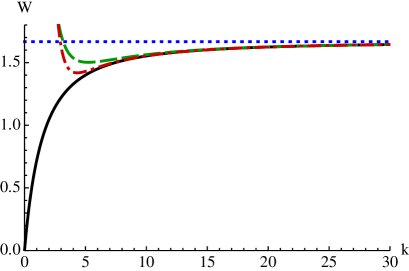
Figure 1: The continuum approximation of $W_{\Box}(\kappa)$ for $q=1/4$: On the left graph different approximations of $W_{\Box}(\kappa)$ are plotted as function of $\kappa$. The dotted blue line is the asymptotic value $\frac{1+q}{1-q}=5/3$. The green dashed line includes the $1/\kappa^{2}$ correction and the red dash-dotted line also the $1/\kappa^{4}$ corrections in (3.15). The full continuum approximation in (3.3) and the numerical evaluation of the sum in (3.2) are the solid black line. The difference between them cannot be seen at this scale, and is plotted in the right graph.

The continuum approximation breaks down, though, for negative $\kappa$, where (3.3) and (3.15) have branch cuts. The origin of this is the infinite number of poles of $W_{\Box}(\kappa)$ at $\kappa=-q^{p/2}-q^{-p/2}$ (3.2). These poles all occur at zeros of $\Xi(\kappa)$ (1.8), so they have no dramatic effect on the integral (3.1). The branch cuts, on the other hand, make the integral ambiguous. It would be interesting to find a workaround to extract the corrections to ${\mathcal{I}}_{\Box}(N)$ beyond the leading large $N$ result (3.5).

4 Fundamental representation at small $N$

To evaluate the index with Wilson loops at finite $N$, one can also expand (3.2) in a power series in $\kappa$

$$W_{\Box}(\kappa)=\sum_{N=1}^{\infty}(-1)^{N+1}\kappa^{N}\sum_{p\in 2\mathbb{Z}+1}\sum_{k=1}^{N}\frac{1}{\operatorname{ch}^{k}p\operatorname{ch}^{N-k}(p+2)}\,.$$ (4.1)

Multiplying by $\Xi(\kappa)$ (1.7) one finds at order $\kappa^{N}$

$$Z(N){\mathcal{I}}_{\Box}(N)=\sum_{n=1}^{N}Z(N-n)(-1)^{n+1}\sum_{p\in 2\mathbb{Z}+1}\sum_{k=1}^{n}\frac{1}{\operatorname{ch}^{k}p\operatorname{ch}^{n-k}(p+2)}\,.$$ (4.2)

Using (1.8) the resulting sums are

$$Z(1)=\sum_{p\in 2\mathbb{Z}+1}\frac{1}{\operatorname{ch}p}\,,\qquad Z(2)=\frac{1}{2}\left(\bigg{(}\sum_{p\in 2\mathbb{Z}+1}\frac{1}{\operatorname{ch}p}\bigg{)}^{2}-\sum_{p\in 2\mathbb{Z}+1}\frac{1}{\operatorname{ch}^{2}p}\right).$$ (4.3)

These sums can be calculated (see the techniques in [20, 3, 4])

$$Z(1)=\frac{kK}{\pi}\,,\quad\sum_{p\in 2\mathbb{Z}+1}\frac{1}{\operatorname{ch}^{2}p}=\frac{KE-(1-k^{2})K^{2}}{\pi^{2}}\,,\quad\sum_{p\in 2\mathbb{Z}+1}\frac{1}{\operatorname{ch}p\operatorname{ch}(p+2)}=\frac{q}{1-q^{2}}\,,$$ (4.4)

where $K$ and $E$ are complete elliptic integrals with modulus $k=\theta_{2}^{2}/\theta_{3}^{2}$.

This gives

$${\mathcal{I}}_{\Box}(2)=\frac{1}{Z(2)}\left(\frac{k^{2}K^{2}}{\pi^{2}}-\frac{KE-(1-k^{2})K^{2}}{\pi^{2}}-\frac{q}{1-q^{2}}\right)=2-\frac{1}{Z(2)}\frac{q}{1-q^{2}}\,,$$ (4.5)

where [3]

$$Z(2)=\frac{K(K-E)}{2\pi^{2}}\,.$$ (4.6)

One can consider higher dimensional representations and $N>2$, but the necessary sums get rather unwieldily.

Appendix A Theta functions

The Jacobi theta function $\vartheta_{3}(z,q)$ is given by the series and product representations as

$$\vartheta_{3}(z,q)=\sum_{n=-\infty}^{\infty}q^{n^{2}}e^{2inz}=\prod_{k=1}^{\infty}\big{(}1-q^{2k}\big{)}\big{(}1+2q^{2k-1}\cos(2z)+q^{4k-2}\big{)},$$ (A.1)

in terms of which the auxiliary theta functions are given by

$$\vartheta_{1}(z,q) =iq^{1/4}e^{-iz}\vartheta_{3}\big{(}z-\tfrac{\pi\tau}{2}-\tfrac{\pi}{2},q\big{)}$$ (A.2)

$$\vartheta_{2}(z,q) =q^{1/4}e^{-iz}\vartheta_{3}\big{(}z-\tfrac{\pi\tau}{2},q\big{)}$$

$$\vartheta_{4}(z,q) =\vartheta_{3}(z-\tfrac{\pi}{2},q)\,.$$

Appendix B Higher order expansions

B.1 Antisymmetric representations

The next few terms in (2.10) which could fit on less than a page in a reasonable font are

$$\det(1+X_{A}R)=\exp\operatorname{Tr}\bigg{[}st\big{(}R-RR_{1}\big{)}-\frac{(st)^{2}}{2}\big{(}R^{2}R_{1}^{2}+R^{2}-4RR_{1}^{2}+2RR_{1}^{2}R_{2}\big{)}$$ (B.1)

$$\quad{}+\frac{(st)^{3}}{3}\big{(}{-}R^{3}R_{1}^{3}+R^{3}+6R^{2}R_{1}^{3}-3R^{2}R_{1}^{2}-6RR_{1}^{3}-6RR_{1}^{3}R_{2}^{2}+6RR_{1}^{2}R_{2}^{2}+6RR_{1}^{3}R_{2}-3RR_{1}^{2}R_{2}^{2}R_{3}\big{)}$$

$$\quad{}-\frac{(st)^{4}}{4}\big{(}R^{4}R_{1}^{4}+R^{4}-8R^{3}R_{1}^{4}+8R^{3}R_{1}^{3}+12R^{2}R_{1}^{4}-8R^{2}R_{1}^{3}+6R^{2}R_{1}^{4}R_{2}^{2}-8R^{2}R_{1}^{3}R_{2}^{2}+4R^{2}R_{1}^{2}R_{2}^{2}$$

$$\qquad{}-8RR_{1}^{4}+8RR_{1}^{4}R_{2}^{3}-16RR_{1}^{3}R_{2}^{3}+8RR_{1}^{2}R_{2}^{3}-24RR_{1}^{4}R_{2}^{2}+16RR_{1}^{3}R_{2}^{2}+8RR_{1}^{2}R_{2}^{3}R_{3}^{2}-8RR_{1}^{2}R_{2}^{2}R_{3}^{2}$$

$$\qquad{}+12RR_{1}^{4}R_{2}+8RR_{1}^{3}R_{2}^{3}R_{3}-16R_{1}^{2}R_{2}^{3}R_{3}+4RR_{1}^{2}R_{2}^{2}R_{3}^{2}R_{4}\big{)}$$

$$\quad{}+\frac{(st)^{5}}{5}\big{(}{-}R^{5}R_{1}^{5}+R^{5}+10R^{4}R_{1}^{5}-15R^{4}R_{1}^{4}-20R^{3}R_{1}^{5}+30R^{3}R_{1}^{4}-5R^{3}R_{1}^{3}+20R^{2}R_{1}^{5}-10R^{2}R_{1}^{4}$$

$$\qquad{}-20R^{2}R_{1}^{5}R_{2}^{3}+40R^{2}R_{1}^{4}R_{2}^{3}-30R^{2}R_{1}^{3}R_{2}^{3}+10R^{2}R_{1}^{2}R_{2}^{3}+30R^{2}R_{1}^{5}R_{2}^{2}-30R^{2}R_{1}^{4}R_{2}^{2}+10R^{2}R_{1}^{3}R_{2}^{2}$$

$$\qquad{}-5R^{2}R_{1}^{3}R_{2}^{3}R_{3}^{2}+10R^{2}R_{1}^{2}R_{2}^{3}R_{3}^{2}-5R^{2}R_{1}^{2}R_{2}^{2}R_{3}^{2}-10RR_{1}^{5}-10RR_{1}^{5}R_{2}^{4}+30RR_{1}^{4}R_{2}^{4}-30RR_{1}^{3}R_{2}^{4}$$

$$\qquad{}+10RR_{1}^{2}R_{2}^{4}+40RR_{1}^{5}R_{2}^{3}-60RR_{1}^{4}R_{2}^{3}+20RR_{1}^{3}R_{2}^{3}-10RR_{1}^{2}R_{2}^{4}R_{3}^{3}+20RR_{1}^{2}R_{2}^{3}R_{3}^{3}-10RR_{1}^{2}R_{2}^{2}R_{3}^{3}$$

$$\qquad{}-60RR_{1}^{5}R_{2}^{2}+30RR_{1}^{4}R_{2}^{2}-30RR_{1}^{3}R_{2}^{4}R_{3}^{2}+30RR_{1}^{2}R_{2}^{4}R_{3}^{2}+40RR_{1}^{3}R_{2}^{3}R_{3}^{2}-20RR_{1}^{2}R_{2}^{3}R_{3}^{2}$$

$$\qquad{}-20RR_{1}^{3}R_{2}^{2}R_{3}^{2}-10RR_{1}^{2}R_{2}^{2}R_{3}^{3}R_{4}^{2}+10RR_{1}^{2}R_{2}^{2}R_{3}^{2}R_{4}^{2}+20RR_{1}^{5}R_{2}-15RR_{1}^{4}R_{2}^{4}R_{3}+60RR_{1}^{3}R_{2}^{4}R_{3}$$

$$\qquad{}-30RR_{1}^{2}R_{2}^{4}R_{3}-20RR_{1}^{3}R_{2}^{3}R_{3}-20RR_{1}^{2}R_{2}^{3}R_{3}^{3}R_{4}+20RR_{1}^{2}R_{2}^{2}R_{3}^{3}R_{4}+10RR_{1}^{2}R_{2}^{3}R_{3}^{2}R_{4}$$

$$\qquad{}-5RR_{1}^{2}R_{2}^{2}R_{3}^{2}R_{4}^{2}R_{5}\big{)}+{\mathcal{O}}\big{(}(st)^{6}\big{)}\bigg{]}.$$

B.2 Symmetric representations

The next few terms in (2.17) are

$$\hskip-11.38109pt\det(1+X_{S}R)=\exp\operatorname{Tr}\bigg{[}st\big{(}R-RR_{1}\big{)}$$ (B.2)

$${}-\frac{(st)^{2}}{2}\big{(}R^{2}R_{1}^{2}-4R^{2}R_{1}+R^{2}+4RR_{1}+2RR_{1}^{2}R_{2}-4RR_{1}R_{2}+2RR_{2}-2R\big{)}$$

$${}+\frac{(st)^{3}}{3}\big{(}{-}R^{3}R_{1}^{3}+6R^{3}R_{1}^{2}-6R^{3}R_{1}+R^{3}-9R^{2}R_{1}^{2}+18R^{2}R_{1}-6R^{2}R_{1}^{3}R_{2}+18R^{2}R_{1}^{2}R_{2}$$

$$\quad{}-18R^{2}R_{1}R_{2}+6R^{2}R_{2}-3R^{2}-9RR_{1}+6RR_{1}^{3}R_{2}-18RR_{1}^{2}R_{2}+18RR_{1}R_{2}-6RR_{2}$$

$$\quad{}-6RR_{1}^{2}R_{3}-3RR_{1}^{2}R_{2}^{2}R_{3}+12RR_{1}R_{3}+12RR_{1}^{2}R_{2}R_{3}-12RR_{1}R_{2}R_{3}-3RR_{3}+3R\big{)}$$

$${}-\frac{(st)^{4}}{4}\big{(}R^{4}R_{1}^{4}-8R^{4}R_{1}^{3}+12R^{4}R_{1}^{2}-8R^{4}R_{1}+R^{4}+16R^{3}R_{1}^{3}-48R^{3}R_{1}^{2}+32R^{3}R_{1}+8R^{3}R_{1}^{4}R_{2}$$

$$\quad{}-32R^{3}R_{1}^{3}R_{2}+48R^{3}R_{1}^{2}R_{2}-32R^{3}R_{1}R_{2}+8R^{3}R_{2}-4R^{3}+36R^{2}R_{1}^{2}+6R^{2}R_{1}^{4}R_{2}^{2}-24R^{2}R_{1}^{3}R_{2}^{2}$$

$$\quad{}+36R^{2}R_{1}^{2}R_{2}^{2}-24R^{2}R_{1}R_{2}^{2}+6R^{2}R_{2}^{2}-48R^{2}R_{1}-24R^{2}R_{1}^{4}R_{2}+96R^{2}R_{1}^{3}R_{2}-144R^{2}R_{1}^{2}R_{2}$$

$$\quad{}+96R^{2}R_{1}R_{2}-24R^{2}R_{2}+8R^{2}R_{1}^{3}R_{3}-24R^{2}R_{1}^{2}R_{3}+8R^{2}R_{1}^{3}R_{2}^{2}R_{3}-24R^{2}R_{1}^{2}R_{2}^{2}R_{3}$$

$$\quad{}+24R^{2}R_{1}R_{2}^{2}R_{3}-4R^{2}R_{2}^{2}R_{3}+24R^{2}R_{1}R_{3}-16R^{2}R_{1}^{3}R_{2}R_{3}+48R^{2}R_{1}^{2}R_{2}R_{3}-48R^{2}R_{1}R_{2}R_{3}$$

$$\quad{}+16R^{2}R_{2}R_{3}-8R^{2}R_{3}+6R^{2}-4RR_{1}^{2}R_{3}^{2}+16RR_{1}+12RR_{1}^{4}R_{2}-48RR_{1}^{3}R_{2}+72RR_{1}^{2}R_{2}$$

$$\quad{}-48RR_{1}R_{2}+12RR_{2}-16RR_{1}^{3}R_{3}+8RR_{1}^{3}R_{2}^{3}R_{3}+48RR_{1}^{2}R_{3}-48RR_{1}^{3}R_{2}^{2}R_{3}+72RR_{1}^{2}R_{2}^{2}R_{3}$$

$$\quad{}-48RR_{1}R_{3}+48RR_{1}^{3}R_{2}R_{3}-144RR_{1}^{2}R_{2}R_{3}+72RR_{1}R_{2}R_{3}+8RR_{3}+8RR_{1}^{2}R_{4}+8RR_{1}^{2}R_{2}^{2}R_{4}$$

$$\quad{}-16RR_{1}R_{2}^{2}R_{4}+4RR_{2}^{2}R_{4}+4RR_{1}^{2}R_{3}^{2}R_{4}+4RR_{1}^{2}R_{2}^{2}R_{3}^{2}R_{4}-8RR_{1}^{2}R_{2}R_{3}^{2}R_{4}-16RR_{1}R_{4}$$

$$\quad{}-16RR_{1}^{2}R_{2}R_{4}+32RR_{1}R_{2}R_{4}-8RR_{2}R_{4}-16RR_{1}^{2}R_{3}R_{4}-16RR_{1}^{2}R_{2}^{2}R_{3}R_{4}+16RR_{1}R_{2}^{2}R_{3}R_{4}$$

$$\quad{}+16RR_{1}R_{3}R_{4}+32RR_{1}^{2}R_{2}R_{3}R_{4}-32RR_{1}R_{2}R_{3}R_{4}+4RR_{4}-4R\big{)}+{\mathcal{O}}\big{(}(st)^{5}\big{)}\bigg{]}.$$

References

- [1] C. Romelsberger, “Counting chiral primaries in , superconformal field theories,” Nucl. Phys. B747 (2006) 329–353, hep-th/0510060.
- [2] J. Kinney, J. M. Maldacena, S. Minwalla, and S. Raju, “An index for dimensional super conformal theories,” Commun. Math. Phys. 275 (2007) 209–254, hep-th/0510251.
- [3] J. Bourdier, N. Drukker, and J. Felix, “The exact Schur index of SYM,” arXiv:1507.08659.
- [4] J. Bourdier, N. Drukker, and J. Felix, “The Schur index from free fermions,”. to appear.
- [5] D. Gang, E. Koh, and K. Lee, “Line operator index on ,” JHEP 05 (2012) 007, arXiv:1201.5539.
- [6] Y. Ito, T. Okuda, and M. Taki, “Line operators on and quantization of the Hitchin moduli space,” JHEP 04 (2012) 010, arXiv:1111.4221.
- [7] N. Mekareeya and D. Rodriguez-Gomez, “5d gauge theories on orbifolds and 4d ‘t Hooft line indices,” JHEP 11 (2013) 157, arXiv:1309.1213.
- [8] F. A. Dolan and H. Osborn, “Applications of the superconformal index for protected operators and -hypergeometric identities to dual theories,” Nucl. Phys. B818 (2009) 137–178, arXiv:0801.4947.
- [9] A. Gadde, E. Pomoni, L. Rastelli, and S. S. Razamat, “-duality and 2d topological QFT,” JHEP 03 (2010) 032, arXiv:0910.2225.
- [10] A. Gadde, L. Rastelli, S. S. Razamat, and W. Yan, “Gauge theories and Macdonald polynomials,” Commun. Math. Phys. 319 (2013) 147–193, arXiv:1110.3740.
- [11] S. S. Razamat, “On a modular property of superconformal theories in four dimensions,” JHEP 10 (2012) 191, arXiv:1208.5056.
- [12] G. Frobenius and L. Stickelberger, “Über die Addition und Multiplication der elliptischen Functionen.,” J. Reine Angew. Math. 88 (1879) 146–184.
- [13] G. Frobenius, “Über die elliptischen Functionen zweiter Art,” J. Reine Angew. Math. 93 (1882) 53–68.
- [14] C. Krattenthaler, “Advanced determinant calculus: a complement,” Linear Algebra Appl. 411 (2005) 68–166, math/0503507.
- [15] M. Mariño and P. Putrov, “ABJM theory as a Fermi gas,” J. Stat. Mech. 1203 (2012) P03001, arXiv:1110.4066.
- [16] A. Klemm, M. Mariño, M. Schiereck, and M. Soroush, “Aharony-Bergman-Jafferis-Maldacena Wilson loops in the Fermi gas approach,” Z. Naturforsch. A68 (2013) 178–209, arXiv:1207.0611.
- [17] Y. Hatsuda, M. Honda, S. Moriyama, and K. Okuyama, “ABJM Wilson loops in arbitrary representations,” JHEP 10 (2013) 168, arXiv:1306.4297.
- [18] S. Hirano, K. Nii, and M. Shigemori, “ABJ Wilson loops and Seiberg duality,” PTEP 2014 no. 11, (2014) 113B04, arXiv:1406.4141.
- [19] H. Ouyang, J.-B. Wu, and J.-j. Zhang, “Exact results for Wilson loops in orbifold ABJM theory,” arXiv:1507.00442.
- [20] I. J. Zucker, “The summation of series of hyperbolic functions,” SIAM J. Math. Anal. 10 no. 1, (1979) 192–206.