Leading QCD Corrections for Indirect Dark Matter Searches: a Fresh Look

Abstract

The annihilation of non-relativistic dark matter particles at tree level can be strongly enhanced by the radiation of an additional gauge boson. This is particularly true for the helicity-suppressed annihilation of Majorana particles, like neutralinos, into fermion pairs. Surprisingly, and despite the potentially large effect due to the strong coupling, this has so far been studied in much less detail for the internal bremsstrahlung of gluons than for photons or electroweak gauge bosons. Here, we aim at bridging that gap by presenting a general analysis of neutralino annihilation into quark anti-quark pairs and a gluon, allowing e.g. for arbitrary neutralino compositions and keeping the leading quark mass dependence at all stages in the calculation. We find in some cases largely enhanced annihilation rates, especially for scenarios with squarks being close to degenerate in mass with the lightest neutralino, but also notable distortions in the associated antiproton and gamma-ray spectra. Both effects significantly impact limits from indirect searches for dark matter and are thus important to be taken into account in, e.g., global scans. For extensive scans, on the other hand, full calculations of QCD corrections are numerically typically too expensive to perform for each point in parameter space. We present here for the first time an efficient, numerically fast implementation of QCD corrections, extendable in a straight-forward way to non-supersymmetric models, which avoids computationally demanding full one-loop calculations or event generator runs and yet fully captures the leading effects relevant for indirect dark matter searches. In this context, we also present updated constraints on dark matter annihilation from cosmic-ray antiproton data. Finally, we comment on the impact of our results on relic density calculations.

I Introduction

The CERN Large Hadron Collider (LHC), now restarted with higher luminosity and center-of-mass energies after the scheduled two years’ shut-down, continues to probe and constrain the electroweak scale for physics beyond the Standard Model (BSM). One of the better motivated BSM frameworks, Supersymmetry (SUSY) Wess and Zumino (1974) has received a lot of attention at the LHC. As such the parameter space for weak scale SUSY is becoming constrained, with minimalistic versions claimed excluded Bechtle et al. (2014); Buchmueller et al. (2014). Given the strong theoretical case for SUSY, and the absence of compelling alternatives, this highlights the importance of moving beyond the simplest case, and considering less constrained but equally well motivated versions of the “Minimal Supersymmetric Standard Model” (MSSM), with more free parameters. Consequently, the community has seen a steadily increasing effort to study such models and their much richer phenomenology, especially in the context of global scans that perform a simultaneous statistical fit to all accounted-for data (for recent examples, see Strege et al. (2014); Cahill-Rowley et al. (2015); Roszkowski et al. (2015); de Vries et al. (2015); Aad et al. (2015a)).

While so far no direct indication for BSM physics has been found at the LHC, clear evidence is provided by the observation of dark matter (DM) in the Universe, if so far only via its gravitational interactions Ade et al. (2015). In weak scale SUSY the lightest supersymmetric particle (LSP) provides an excellent candidate for DM Jungman et al. (1996). The most often studied situation, which we will also consider here, is an LSP given by the lightest neutralino. In fact, this provides a very useful template for the much more general class of weakly interacting massive particles (WIMPs), which are characterized by an interaction cross section with Standard Model states in the right range to be a thermal relic that fully accounts for the observed DM abundance today Bertone et al. (2005). Such WIMPs can be searched for not only at colliders, but also in direct detection experiments looking for the recoil off target nuclei in large underground detectors, or indirect searches looking for WIMP annihilation products in the observed astrophysical fluxes of gamma rays or charged cosmic rays like antiprotons. Both direct Akerib et al. (2014) and indirect Ackermann et al. (2015); Bergström et al. (2013) searches now start to place severe limits on the simplest WIMP models, which makes astrophysical searches for DM interactions a promising avenue for discovery of new physics that is complementary to searches at the LHC.

Within the MSSM there is the interesting possibility of coannihilating DM Edsjö and Gondolo (1997); Ellis et al. (2000), in which the LSP and next-to-lightest supersymmetric particle (NLSP) are near degenerate in mass and (co-)annihilations of the NLSP (and potentially other particles only slightly heavier than the NLSP) are the decisive processes to determine the DM relic abundance. Scenarios with almost degenerate squark NLSPs, in particular, tend to constitute blind spots in LHC searches: even if created with relatively high rates such NLSPs produce jets in their decay that are too soft to pass the cuts Kawagoe and Nojiri (2006), thereby generally evading current bounds from direct squark searches (as long as other, heavier states are out of reach for the available energy and luminosity; though monojet searches may help to fill that gap Arbey et al. (2015) and in some models flavour violating stop decays may be enhanced Boehm et al. (2000a); Agrawal and Frugiuele (2014); Blanke et al. (2013)). For light first generation squarks, and to some extent second generation squarks, direct searches therefore provide a powerful complementary tool to test such scenarios Hisano et al. (2011); Garny et al. (2012a). Independent of generation, indirect searches are also very promising in this respect Asano et al. (2012), the reason being that internal bremsstrahlung (IB) processes with an additional gluon in the final state can lift the well known helicity suppression of zero velocity neutralino annihilation.

Figure 1: Annihilation of neutralinos into $\bar{q}q$ from the point of view of an effective interaction. In this article, we focus on leading QCD corrections of this diagram that are relevant for indirect DM searches.

In this article we carefully investigate the general importance of gluon IB in the context of indirect DM searches, by calculating the leading QCD corrections to the process shown schematically in Fig. 1. We perform our calculations for general MSSM scenarios, allowing in particular for arbitrary neutralino compositions and keeping the full quark mass dependence for gluon IB, i.e. $\chi\chi\to\bar{q}qg$. For loop corrections to the process $\chi\chi\to\bar{q}q$, which contribute to radiative corrections of the total annihilation cross section at the same order in the strong coupling $\alpha_{s}$, we adopt a simplified description that fully captures the leading effects but is considerably easier to implement and numerically much faster. While we focus here for definiteness on the MSSM, our method is sufficiently general to be applicable to any BSM model that contains colored new states close in mass to the DM particle. As an important application, this allows to include QCD corrections in a both fast and relatively simple way even in extensive global scans. As we will see, this is particularly relevant for scenarios where parts of the parameter space contain ‘squarks’ almost degenerate in mass with the DM particle.

This article is organized as follows. In Section II we discuss the annihilation of neutralinos into $\bar{q}q$ and $\bar{q}qg$ final states, and sketch the calculational methods that are employed (technical details being deferred to Appendix A). Section III is concerned with the impact on indirect DM searches, including in particular a careful discussion of how DM induced cosmic-ray antiproton and gamma-ray spectra change by including $\bar{q}qg$ processes (for more details, see Appendix B). In Section IV we discuss the effect of gluon bremsstrahlung processes on relic abundance calculations in supersymmetric models. We present our conclusions in Section V.

II Neutralino annihilation into $\bar{q}qg$

We consider the minimal supersymmetric standard model (MSSM), where the four neutralinos are a linear combination of the superpartners of the neutral Higgs bosons and gauge fields,

$$\chi_{i}^{0}=N_{i1}\tilde{B}+N_{i2}\tilde{W}^{3}+N_{i3}\tilde{H}_{1}^{0}+N_{i4}\tilde{H}_{2}^{0}\,.$$ (1)

Throughout, we will refer to the lightest of these Majorana fermions simply as the neutralino, $\chi\equiv\chi^{0}_{1}$. As schematically depicted in Fig. 1, we will be concerned with non-relativistic neutralino annihilation to quarks (or, more specifically, with the $s$-wave part of the annihilation cross section). At tree level, more specifically, this process is determined by the contributions shown in Fig. 2: $s$-channel exchange of a $Z$ or pseudo-scalar Higgs boson, as well as $t$-channel squark exchange.

Figure 2: $s$-wave neutralino annihilation into quark anti-quark pairs proceeds through $Z$ boson, pseudo-scalar Higgs $A$ and squark $\tilde{q}$ exchange.

For non-relativistic relative velocities $v$ of the incoming DM particles, the annihilation cross section can be well approximated by expanding $\sigma v\simeq a_{0}+a_{1}v^{2}$. With Galactic velocities of $v\sim 10^{-3}$, annihilation in the Milky Way halo is thus typically dominated by $s$-wave contributions and given by $\sigma v\simeq a_{0}$. For Majorana DM the requirement that the annihilating pair be even under charge conjugation implies that the initial state in Figs. 1 and 2 transforms as a pseudo scalar under Lorentz transformations in the $v\to 0$ limit ($0^{-+}$ in $J^{PC}$ notation, see e.g. Ref. Weiler (2012) for a recent comprehensive discussion). This requirement causes $s$-wave annihilations into $\bar{q}q$ to become helicity suppressed, scaling as $\sigma v\propto m_{q}^{2}/m_{\chi}^{2}$. As first noted in Refs. Bergström (1989); Flores et al. (1989), the helicity suppression can be lifted by radiating a gauge boson from an internal propagator (hence later coined ‘virtual’ internal bremsstrahlung Bringmann et al. (2008), VIB). The resulting enhancement of the annihilation rate is maximal for a $t$-channel particle degenerate in mass with the neutralino, $\sigma_{\mathrm{3body}}/\sigma_{\mathrm{2body}}\sim(\alpha_{\mathrm{em}}/\pi)\,m_{\chi}^{2}/m_{q}^{2}$, and becomes suppressed by a factor of roughly 2 (3) for a mass difference of 10% (20%) Bergström et al. (2008). Subsequently, the impact of IB was studied in great detail for both photons Baltz and Bergström (2003); Beacom et al. (2005); Bringmann et al. (2008); Bell and Jacques (2009); Bergström et al. (2008); Barger et al. (2009); Bringmann et al. (2012); Bergström (2012); Garny et al. (2013); Toma (2013); Giacchino et al. (2013) and electroweak gauge bosons Kachelriess et al. (2009); Bell et al. (2011a); Yaguna (2010); Bell et al. (2011b); Ciafaloni et al. (2011a); Bell et al. (2011c); Garny et al. (2011); Ciafaloni et al. (2011b, 2012); Fukushima et al. (2012); Bell et al. (2012); Bringmann and Calore (2014). Given the nature of strong interactions, one should expect the effect to be even more pronounced for gluon internal bremsstrahlung in the case of quark final states, $\chi\chi\rightarrow\bar{q}qg$. Pictured in Fig. 3, however, this process has typically only been studied in the limit of $m_{q}\sim 0$ or for various simplifying assumptions concerning the neutralino composition and couplings (see, e.g., Refs. Drees et al. (1994); Asano et al. (2012); Garny et al. (2012b, a)). The purpose of this work is therefore to treat gluon IB more generally, in particular by allowing for arbitrary neutralino compositions and by considering heavier quarks.

Figure 3: Gluon internal bremsstrahlung, left to right: final state radiation, FSR, off $q$, off $\bar{q}$ and virtual internal bremsstrahlung, VIB. See Appendices A and B for a proper, and manifestly gauge-invariant, description of this naive distinction between FSR and VIB.

The differential cross section for the process $\chi\chi\to\bar{f}f\gamma$, in the $v=0$ limit, has been calculated in full generality in Ref. Bringmann et al. (2008). Accounting for the proper contraction of $SU(3)$ generators, the differential cross section for $\chi\chi\to\bar{q}qg$ is then readily obtained by the simple rescaling

$$Q^{2}\alpha_{\mathrm{em}}\to\frac{4}{3}\alpha_{\mathrm{s}}\,,$$ (2)

where $Q$ is the electric charge of the quark. For down-type quarks, we thus naively expect an effect of the order of $12\alpha_{\mathrm{s}}/\alpha_{\mathrm{em}}=\mathcal{O}(10^{2})$ larger for gluon than for photon emission. As a consequence, the total neutralino annihilation rate (including other final states than quarks) is also likely affected in a significant way. This should be contrasted to the much better studied case of QED, where light fermion final states typically contribute only sub-dominantly even when taking into account IB: rather than enhancing the total annihilation rate, the main phenomenological significance of photon VIB thus consists in the appearance of distinct spectral features in gamma rays and positrons, at $E\sim m_{\chi}$ Bringmann et al. (2012); Bergström et al. (2008). In the QCD case this is different because of the expected size of the effect, but also because the additional final-state gluon will fragment with a high multiplicity into lower-energy particles, thus smearing out any spectral features potentially observable in cosmic rays (see however the discussion in Section III).

The need to calculate the total integrated, rather than only the differential cross section adds a complication because of the well-known infrared divergence associated to the emission of massless gauge bosons. This divergence is canceled by $\mathcal{O}(\alpha_{s})$ interference terms between the diagrams in Fig. 2, and 1-loop corrections to the simplified tree-level process pictured in Fig. 1. More specifically the relevant diagrams are shown in Fig. 4, where the blob represents the sum over all processes in Fig. 2, and the cross represents the sum over all counterterms required to cancel ultraviolet (UV) divergences present in the left diagram. As discussed in more detail in Appendix A, we will adopt a simplified model approach, where we only keep the terms corresponding to those diagrams. Compared to full next-to-leading (NLO) calculations at $\mathcal{O}(\alpha_{s})$, see e.g. Refs. Herrmann and Klasen (2007); Herrmann et al. (2009a, b, 2014), this neglects diagrams containing gluinos and squark self-energies, as well as supersymmetric corrections to the quark self-energy and the neutralino-squark-quark coupling. These diagrams, however, are typically subdominant as none of them can lift the helicity suppression of the tree-level annihilation. Our simplified approach thus exactly reproduces the full NLO result in particular for SUSY models in which gluon bremsstrahlung processes are dominant. This is the generic situation for light quarks in the final state, and squarks not much heavier than the neutralino.

Figure 4: 1-loop correction to Fig. 2 (left), Sum of counterterm diagrams for all processes contributing to Fig. 2 (right).

III Indirect dark matter searches with gamma rays and cosmic-ray antiprotons

Figure 5: Top panels. Antiproton spectra from $\bar{q}q$ (dashed) and $\bar{q}qg$ (solid) for $m_{\chi}=100$ GeV and both $u$ (left) and $b$ (right) quarks. For the 3-body case, a simplified gluon VIB distribution is assumed, with $m_{\chi}=m_{\tilde{b}}$ and vanishing squark mixing. Bottom panels. Same, but for photon spectra. All spectra are normalized such as to give the differential number $N$ of antiprotons or photons per neutralino pair annihilation into 2-body or (FSR-subtracted) 3-body final states, respectively, c.f. Eq. (31). The high energy feature visible in the $\bar{b}b$ antiproton spectra is due to decaying $B^{0}$ mesons.

In view of the small Galactic velocities, indirect searches for DM provide the ideal testbed for large effects on the annihilation rate of neutralino DM in the zero velocity limit. In general, the final state quarks and gluons from DM annihilation in the Galactic halo will fragment and decay, and thereby eventually contribute to the observed flux in charged and neutral cosmic rays. Of special interest in this context are gamma rays Bringmann and Weniger (2012), with very robust limits in particular provided by Fermi observations of dwarf spheroidal galaxies Ackermann et al. (2015), and antiprotons which are produced in large quantities from the $\bar{q}qg$ final states we focus on here.

III.1 Energy spectrum from neutralino annihilation

We simulate parton showering and hadronization of $\bar{q}q$ and $\bar{q}qg$ final states using PYTHIA 8.2 Sjöstrand et al. (2008); Sjostrand et al. (2006), setting the center of momentum energy to be $2m_{\chi}$. For three-body final states, the resulting energy spectrum for photons and antiprotons $dN/dT$ (with $T$ denoting kinetic energy) is then derived by randomly sampling from the full gluon and quark energy distribution $d^{2}\tilde{N}_{\bar{q}qg}/dE_{g}dE_{q}$, obtained from Ref. Bringmann et al. (2008) after rescaling as in Eq. (2) and with FSR processes subtracted to avoid double counting (for quantities we denote with a tilde, the FSR contribution is always understood to be subtracted; see Appendix A and B for details). To produce the expected spectra, we performed $10^{7}$ Pythia runs for each quark channel, resulting in an accuracy of $\lesssim$ 1% at the energies of interest.

For both antiproton and gamma ray spectra, there turns out to be substantial difference between $\bar{q}q$ and $\bar{q}qg$ final states; the main effect being that the fragmentation of the additional gluon in the final state significantly enhances the yields at small energies while slightly depleting it at higher energies (which indeed is expected as a result of the on average higher multiplicity in the final state). We illustrate this in Fig. 5, where we compare the spectra of antiprotons and photons resulting from $\bar{b}b$ and $\bar{b}bg$, and $\bar{u}u$ and $\bar{u}ug$ final states, for an assumed DM mass of $m_{\chi}=100$ GeV. The high-energy feature visible in the $\bar{b}b$ spectra is a direct result of the decay of heavy $b$ states such as $B^{0}$ mesons, and is clearly absent in $\bar{u}u$ and $\bar{u}ug$ processes. For the displayed $\bar{q}qg$ final states, we choose the “maximal” VIB case, obtained for large squark mixing as defined by Eq. (34). We found that this maximal VIB case leads to the largest possible difference between antiproton (or photon) spectra from $\bar{q}qg$ and $\bar{q}q$ final states, respectively.

$\bar{q}q$	$g_{\tilde{q}i}^{\textrm{r}}$	$c_{1}$	$c_{2}$	$c_{3}$	$n_{1}$	$n_{2}$	$n_{3}$
$\bar{c}c$	$\geq 10^{-4}$	-0.13	5.35	-5.22	0	9.8	9.15
$\bar{s}s$	$\geq 10^{-4}$	-0.4	-9.14	9.54	0	8.1	9.98
$\bar{t}t$	$\geq 10^{-4}$	-0.67	-2.41	3.08	0	0.43	0.27
$\bar{b}b$	$\geq 10^{-4}$	8.1	-8.32	0.22	0	0.02	9.53
$\bar{t}t$	$<10^{-4}$	0.1	0.21	-0.31	0	8.73	5.53

Table 1: Coefficients to obtain the antiproton spectrum from $\bar{q}qg$ final states for any MSSM model as linear combination of “$m_{\tilde{q}}\rightarrow\infty$” and “maximal VIB” $\bar{q}qg$ spectra for both large squark mixing ($g_{\tilde{q}i}^{\textrm{r}}\geq 10^{-4}$, first three rows) and small squark mixing ($g_{\tilde{q}i}^{\textrm{r}}<10^{-4}$, last row). See Eqns. (3-6) for a full discussion. Note that the parameters $c_{i}$ and $n_{i}$ are, within the uncertainties discussed in the main text, independent of the neutralino mass for $10\,\mathrm{GeV}\lesssim m_{\chi}\lesssim 10\mathrm{TeV}$. For small squark mixing and all quarks lighter than $t$, the true spectrum is always well approximated by a pure VIB spectrum.

The antiproton and gamma-ray spectra from $\bar{q}qg$ final states are in general model dependent, however, and therefore need to be determined on a model by model basis. This quickly becomes impractical, in particular when scanning over large numbers of models. Fortunately, we can circumvent this issue in an elegant way by approximating the full spectrum as the linear combination of the two extreme cases outlined in Appendix B, i.e. the $\bar{q}qg$ spectrum which is most different from $dN_{\bar{q}q}/dT$, given by the maximal VIB case already mentioned, and the $\bar{q}qg$ spectrum closest to $dN_{\bar{q}q}/dT$, the heavy sfermion limit given in Eq. (37). Explicitly:

$$\frac{d\tilde{N}_{\mathrm{\bar{q}qg}}}{dT_{\bar{p}}} \simeq y_{\bar{p}}\frac{d\tilde{N}_{\bar{q}qg}^{\mathrm{VIB}}}{dT_{\bar{p}}}+(1-y_{\bar{p}})\frac{d\tilde{N}_{\bar{q}qg}^{m_{\tilde{q}}\to\infty}}{dT_{\bar{p}}}\,,$$ (3)

$$\frac{d\tilde{N}_{\mathrm{\bar{q}qg}}}{dE_{\gamma}} \simeq y_{\gamma}\frac{d\tilde{N}_{\bar{q}qg}^{\mathrm{VIB}}}{dE_{\gamma}}+(1-y_{\gamma})\frac{d\tilde{N}_{\bar{q}qg}^{m_{\tilde{q}}\to\infty}}{dE_{\gamma}}\,,$$ (4)

with $y_{i}\in[0,1]$. If, on the other hand, the squarks are essentially unmixed, we interpolate instead between the extreme spectra obtained in that limit; i.e. we use Eqs. (36, 38) rather than (34, 37). We established that this simple proscription indeed describes the real spectrum to an excellent precision, with the scaling parameter $y$ only dependent on the likelihood that the gluon is emitted with a high energy. More precisely, we define

$$r\equiv\frac{r^{\prime}_{\textrm{true}}-r^{\prime}_{\tilde{m}\rightarrow\infty}}{r^{\prime}_{\textrm{VIB}}-r^{\prime}_{\tilde{m}\rightarrow\infty}}\,,$$ (5)

where $r^{\prime}_{\textrm{X}}=dN_{\bar{q}qg}^{\textrm{X}}(x_{\textrm{max}})/dx_{g}$ and $x_{\textrm{max}}$ maximizes the gluon energy spectrum. While somewhat arbitrary, $r$ is a reasonable measure of the relative importance of the pure VIB and VIB/FSR mixing terms in the amplitude squared, which after the subtraction procedure described in detail in Appendix B, dominate the maximal VIB and heavy sfermion spectra respectively.

For a large set of randomized MSSM model parameters, and neutralino masses in the range from 10 GeV to 10 TeV, we then fit Eqs. (3, 4) to the true 3-body antiproton or photon spectrum obtained from Pythia, using

$$\log_{10}(y)=\log_{10}(r)+\sum_{i}c_{i}r^{n_{i}}\,.$$ (6)

The result for the parameters $c_{i}$ and $n_{i}$ are shown in Tables 1 and 2. The contribution to the gluon energy spectrum from VIB/FSR mixing terms is proportional to the quark mass, and therefore expected to be suppressed relative to the purely VIB contribution for lighter quarks. In fact we find that in the mixed case for $u$ and $d$ quarks, and in the unmixed case for all quarks but the top, that $y(r)\simeq 1$ for $r\ll 0.1$ when fitting the antiproton/gamma-ray spectra. We therefore assume $y=1$ in these cases for simplicity.

$\bar{q}q$	$g_{\tilde{q}i}^{\textrm{r}}$	$c_{1}$	$c_{2}$	$c_{3}$	$n_{1}$	$n_{2}$	$n_{3}$
$\bar{c}c$	$\geq 10^{-4}$	0.03	-7.97	7.94	0	8.08	9.83
$\bar{s}s$	$\geq 10^{-4}$	0.12	-8.24	8.12	0	7.05	9.63
$\bar{t}t$	$\geq 10^{-4}$	-4.8	6.44	-1.64	0	0.06	0.34
$\bar{b}b$	$\geq 10^{-4}$	0.26	3.89	-4.15	0	2.22	1.63
$\bar{t}t$	$<10^{-4}$	0.08	1.05	-1.13	0	8.36	7.45

Table 2: Same as Tab. 1, but for gamma-ray spectra.

    

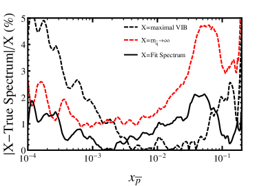
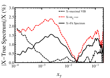
Figure 6: Deviation from true antiproton (left) and gamma-ray (right) spectra for $\bar{b}bg$ VIB (dashed black), $\bar{b}bg$ $m_{\tilde{q}}\rightarrow\infty$ (dashed red) and $\bar{b}bg$ fitted (solid black), coming from a pMSSM-7 model with parameters $M_{1}=2.95$ TeV, $M_{2}=4.96$ TeV, $\mu=2.41$ TeV, $m_{A}=10$ TeV, $\tan\beta=14.77$, $A_{t}/M_{1}=1.218$ and $A_{b}/M_{1}=2.532$. This models features a mixed Higgsino-Bino lightest neutralino with mass $m_{\chi}=2.49$ TeV, and a relatively large sbottom mixing; both relic density and Higss mass are consistent with observational constraints.

For the models tested this procedure was found to reproduce the true gamma-ray spectra from $\bar{q}qg$ to within 2% for $E_{\gamma}<10^{-3}m_{\chi}$, 5% for $10^{-3}m_{\chi}<E_{\gamma}<0.2m_{\chi}$ and within 8% for higher energies. For antiprotons the accuracy is within 10% for $T_{\bar{p}}<10^{-2}\,m_{\chi}$, 8% for $10^{-2}\,m_{\chi}<T_{\bar{p}}<0.2\,m_{\chi}$, and to within 20% for higher energies. We note that the relatively large deviation in particular at high energies is likely a result of models with intermediate squark mixings, i.e. $g_{\tilde{q}i}^{\textrm{r}}\sim 10^{-4}$, which constitutes the worst point in both mixed and unmixed fits. In fact, for models away from the intermediate mixing region – corresponding to the bulk of models tested – the above errors are overly pessimistic, reducing to 3% for $10^{-3}m_{\chi}<E_{\gamma}<0.2m_{\chi}$ and 5% for $10^{-2}m_{\chi}<T_{\bar{p}}<0.2m_{\chi}$. As a possible future improvement on this procedure, one may use the values of the couplings to interpolate smoothly between the $g^{L}_{\tilde{q}Lq\chi}=g^{R}_{\tilde{q}Rq\chi}$ and $g^{L}_{\tilde{q}Rq\chi}=g^{R}_{\tilde{q}Rq\chi}=0$ extreme spectra, thereby improving the fit at very high energies at the expense of introducing one more fitting parameter. Above $E_{\gamma}/T_{\bar{p}}\sim 0.5m_{\chi}$, furthermore, the reliability of simulated spectra decreases to around the 20% level due to the limited statistics of event generations, independent of the accuracy of the fit. The errors associated with the fit of the function $y(r)$ itself are at worst of the order of $0.3$; this results, by using Eqs. (3, 4), in uncertainties in the spectra at the same order or smaller than the uncertainties discussed above. For illustration, we show in Fig. 6 the percent difference between a spectrum fitted using the above procedure, and an MSSM model with a neutralino of mass $2.488$ TeV, explicitly simulated for this particular model using Pythia.

We conclude this Section by stressing that the parameterization given in Eqs. (3–6) provides one of our main results. It allows to compute antiproton and photon spectra from leading QCD corrections directly from tabulated ‘extreme’ 3-body spectra – obtained in the heavy sfermion and maximal VIB limit, respectively – without having to run an event generator like Pythia for each model. As argued above, this is a highly desirable property in terms of computational performance which makes it very convenient for future applications, in particular in the context of large parameter scans. Our antiproton and gamma-ray yield routines, including the yield tables for gluon VIB and heavy sfermion IB, have been fully implemented in DarkSUSY Gondolo et al. (2004); *dsweb and will be available with the next public release. Concretely, we tabulated mixed/ unmixed VIB and $m_{\tilde{q}}\rightarrow\infty$ antiproton $d\tilde{N}_{\bar{q}qg}/dT_{\bar{p}}$ and gamma-ray spectra $d\tilde{N}_{\bar{q}qg}/dE_{\gamma}$ for all quarks, and for 100 dark matter masses in the range 5 GeV–10 TeV. For a given MSSM model, our numerical routines then interpolate the expected VIB and $\tilde{m}\rightarrow\infty$ spectra between the discrete values of neutralino masses explicitly simulated, and weigh them according to Eqs. (3, 4). Overall, this procedure reproduces the true antiproton/gamma ray spectrum to an accuracy better than $\sim 10\%$ for $T_{\bar{p}}/E_{\gamma}<0.2m_{\chi}$, being as good as $\sim 3\%$ in the energy range $10^{-3}m_{\chi}<T_{\bar{p}}/E_{\gamma}<0.2m_{\chi}$, as stipulated above.

III.2 Gamma-ray and antiproton constraints

While gamma rays propagate essentially unperturbed through the Galaxy, antiprotons are deflected by Galactic magnetic field inhomogeneities. The resulting motion can effectively be described as a random walk, and thus by a diffusion equation in momentum space Ginzburg and Syrovatskii (1964). In the following, we use the same prescription as adopted in Ref. Bringmann et al. (2014) to derive limits on a dark matter annihilation signal in antiprotons. For the astrophysical background, we thus use a three-parameter model to take into account the effect of solar modulation via a freely varying force field parameter $\phi_{F}$ Gleeson and Axford (1968); Perko (1987), and to interpolate between available extreme predictions obtained due to propagation model Bringmann and Salati (2007) and nuclear cross section uncertainties Donato et al. (2001). The antiproton flux from DM, on the other hand, depends to a much larger degree on the choice of propagation model than the astrophysical background; here, we use the recommended reference model, ’KRA’, of the comprehensive analysis presented in Ref. Evoli et al. (2012). Finally, we obtain limits on the signal by means of a likelihood ratio test Rolke et al. (2005) against the PAMELA data Adriani et al. (2013), where we profile over all parameters other than the signal normalization (noting that data from the AMS-02 experiment are still preliminary Talk at the ‘AMS Days at CERN’ (2015)). For further details of the procedure adopted, we refer the reader to Ref. Bringmann et al. (2014). In Fig. 7, we show the resulting limits on the annihilation rate into quark-antiquark pairs.

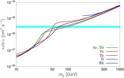
Figure 7: Updated limits on the DM annihilation rate into quark pairs, derived from cosmic-ray antiproton data. The cyan area gives a rough indication of the cross section required for thermal DM production. See text for further details.

In Fig. 8, we illustrate how these limits change when considering $\bar{q}qg$ rather than $\bar{q}q$ final states. Here, we adopt for illustration the mixed VIB spectrum for the case of $\bar{q}qg$ final states, see Eq. (34), with a normalization that corresponds to the same cross section for 3- and 2-body final states, i.e. ${\tilde{\sigma}_{\bar{q}qg}}={\sigma_{0}^{\mathrm{full}}}$. The displayed improvement in the antiproton limits by a factor of up to $\sim$5 therefore results exclusively from the change in the antiproton spectrum; the actual limit improvement, for a given SUSY model, will be larger by another factor of up to ${\tilde{\sigma}_{\bar{q}qg}}/{\sigma_{0}^{\mathrm{full}}}\lesssim(\alpha_{\mathrm{s}}/\pi)(m_{\chi}/m_{q})^{2}$. Let us stress that the displayed ratios of limits are rather insensitive to the choice of propagation model (as opposed to the limits themselves, see Fig. 7). Taken together, this implies that gluon IB can indeed have a rather sizable impact on indirect searches for Majorana DM particles annihilating into quarks.

To further illustrate this, let us consider a pure Bino DM candidate with $m_{b}\ll m_{\tilde{B}}<m_{t}$ and all squarks exactly degenerate in mass $\tilde{B}$. The total annihilation cross section into all $\bar{q}qg$ final states is then given by Asano et al. (2012)

$${\tilde{\sigma}_{\bar{q}qg}}^{\mathrm{Bino}}v = \frac{\alpha_{\rm s}\alpha^{2}_{Y}}{m_{\tilde{B}}^{2}}\frac{565}{1944}\left(21-2\pi^{2}\right)$$ (7)

$$= 5.2\times 10^{-27}\left(\frac{m_{\tilde{B}}}{100\,\mathrm{GeV}}\right)^{-2}\,\mathrm{cm}^{3}\,\mathrm{s}^{-1}\,.$$

On top of that we also add the contribution from gluon pair final states Bergstrom and Snellman (1988); Drees et al. (1994). Just as for single quark channels, the shape of the combined antiproton spectrum from Bino annihilation changes significantly when including QCD corrections. As indicated in Fig. 8, this improves antiproton limits by a factor of up to 2.7 compared to the ‘standard’ spectrum resulting from $\bar{b}b$ final states. For the reference propagation model (‘KRA’), we find that such a scenario can be excluded from antiproton data up to $m_{\tilde{B}}\sim$ 61 GeV. Allowing a larger size of the diffusive halo, as realized in the ‘MAX’ propagation model Donato et al. (2004), even Bino and (exactly degenerate) squark masses below about 92 GeV would be excluded. Experiments with improved statistics, like AMS-02, will be even more sensitive to the spectral shape of the antiproton spectrum, and hence help to push these limits to even higher masses.

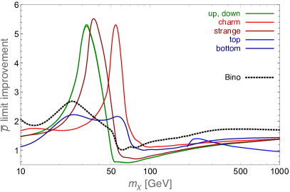
Figure 8: Ratio of antiproton limits on the total annihilation rate $\sigma v$ into VIB $\bar{q}qg$ vs. $\bar{q}q$ final states, as a function of the neutralino mass $m_{\chi}$ and assuming the same cross section for $\bar{q}qg$ and $\bar{q}q$. The actual improvement in the limits will thus be larger by a factor of up to about $(\alpha_{\mathrm{s}}/\pi)(m_{\chi}/m_{q})^{2}$. Note that while the limits themselves (derived by the same procedure as adopted in Ref. Bringmann et al. (2014)) strongly depend on the adopted propagation model, the displayed ratios are rather insensitive to this choice. The dotted line shows the case of a pure Bino and exactly degenerate squarks, see discussion after Eq. (7), as compared to a spectrum resulting from $\bar{b}b$ final states. Note that $\bar{q}qg$ final states are relevant in particular for squarks highly degenerate in mass with the neutralino; in such scenarios even neutralino masses well below 100 GeV can evade constraints from LEP Achard et al. (2004); Group (2004) or the LHC Aad et al. (2014, 2015b).

This clearly highlights the complementarity between indirect searches for DM and collider searches: While direct searches for squarks at the LHC have produced impressive limits reaching up to the TeV scale Aad et al. (2014, 2015c); Chatrchyan et al. (2014), it is crucial to remember that those limits do not apply to highly mass-degenerate scenarios. In fact, even first and second generation squarks with $m_{\tilde{q}}\lesssim$ 100  GeV still remain unconstrained from such searches unless the squark to neutralino mass ratio is considerably higher than 10% Aad et al. (2014). Also earlier data from the large electron-positron collider (LEP) only constrain scenarios where the squarks are at least a few percent heavier than the neutralino Achard et al. (2004). Third generation squarks are typically even harder to probe, both at the LHC Aad et al. (2015b) and previously at LEP Group (2004). Below $m_{\chi}\sim m_{Z}/2\sim 46$ GeV, contributions to the $Z$ boson width typically provide the strongest constraints Olive et al. (2014); while independent of $m_{\tilde{q}}$, however, those limits still depend on the neutralino composition.

Figure 9: Same as Fig. 8, but for gamma-ray limits obtained by comparing the photon count above 0.1 GeV. Also in this case the actual improvement in the limits will be larger by another factor of up to about $(\alpha_{\mathrm{s}}/\pi)(m_{\chi}/m_{q})^{2}$. Top quarks feature qualitatively different spectra compared to all other quarks, both for 2-body and 3-body final states, the reason being that top quarks are treated as decaying resonances in PYTHIA 8 (rather than as allowed final states).

Similarly, gamma-ray limits are affected – even though, as discussed above, the spectra do not change as much as in the antiproton case. A full spectral analysis would in general depend on both the specific gamma-ray telescope and the form of the astrophysical backgrounds for the target in question, and hence be clearly beyond the scope of this work. For subdominant backgrounds, however, a very rough estimate of the effect can be obtained by simply comparing the integrated photon spectra from $\bar{q}qg$ and $\bar{q}q$ final states. As an illustrative example let us consider the photon count above 0.1 GeV, indicative of the lower energy threshold of the large area telescope (LAT) on board the Fermi satellite Atwood et al. (2009). In Fig. 9, we show the ratio of this quantity for various quark final states. As anticipated, the enhancement is smaller than in the antiproton case. Still it is not negligible, in particular for large DM masses. The additional expected enhancement of ${\tilde{\sigma}_{\bar{q}qg}}/{\sigma_{0}^{\mathrm{full}}}\lesssim(\alpha_{\mathrm{s}}/\pi)(m_{\chi}/m_{q})^{2}$, furthermore, is of course the same. This makes the QCD corrections computed here highly relevant also for gamma rays, the ‘golden channel’ Bringmann and Weniger (2012) of indirect DM searches.

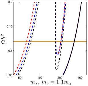
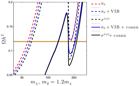
Figure 10: Variation of $\Omega h^{2}$ vs $m_{\chi}$ for a pure Bino model. Left panel: common squark mass of $m_{\tilde{q}}=1.1m_{\chi}$, right panel: $m_{\tilde{q}}=1.2m_{\chi}$. The tree-level annihilation cross section is denoted by $\sigma_{0}$, while $\sigma^{\mathrm{full}}$ contains all relevant QCD corrections; this includes the simplified model NLO corrections contained in $\sigma_{\textrm{tot}}^{\textrm{simp}}$, c.f. Eq. (26), the VIB cross section $\tilde{\sigma}_{\overline{q}qg}$ and the annihilation rate to two gluons. The brown band shows the $1\sigma$ limits on the DM density as observed by Planck Ade et al. (2015). For smaller $m_{\chi}$, the dominant impact of the QCD corrections studied here is due to the VIB contributions, though gluon pair production plays an almost equal role. Near the top threshold, the dominant change is instead related to the simplified model NLO corrections to the two-body rate. For $m_{\tilde{q}}\lesssim 1.1m_{\chi}$, both contributions are negligible compared to the impact of squark co-annihilations.

IV Relic Abundance

As a second application to the leading radiative corrections we have computed here, we consider next the relic density of thermally produced neutralino dark matter. The standard method Gondolo and Gelmini (1991) to compute it, as implemented e.g. in DarkSUSY Gondolo et al. (2004); *dsweb, is to solve the Boltzmann equation for the neutralino number density $n_{\chi}$:

$$\partial_{t}n_{\chi}+3Hn_{\chi}=-\langle\sigma v\rangle_{\mathrm{eff}}\left(n_{\chi}^{2}-{n_{\chi}^{\mathrm{eq}}}^{2}\right)\,.$$ (8)

Here, $H$ denotes the Hubble rate, $\langle\sigma v\rangle_{\mathrm{eff}}$ the thermally averaged annihilation rate including co-annihilations Edsjö and Gondolo (1997), and $n_{\chi}^{\mathrm{eq}}$ the neutralino number density in thermal equilibrium. As before, we will use the simplified approach discussed in Appendix A to calculate the annihilation cross section for neutralinos. Concretely, we include the full QCD-corrected cross section $\sigma_{\textrm{tot}}^{\textrm{simp}}$ of the simplified model, c.f. Eqs. (26) and (30), as well as the FSR- subtracted VIB cross section ($\tilde{\sigma}_{\overline{q}qg}$, see Appendix A.2) at zero velocity, and add them to the relic density routines of DarkSUSY.

For the computation of the neutralino relic density, it generally suffices to know $\langle\sigma v\rangle_{\mathrm{eff}}$ at temperatures relatively close to chemical decoupling, i.e. $\langle\sigma v\rangle_{\mathrm{eff}}\sim Hn_{\chi}$ (unless one encounters complications, like in the case of the Sommerfeld effect for TeV neutralino masses Hisano et al. (2007); Hryczuk et al. (2011); Hryczuk (2011)). For typical decoupling temperatures $T\sim m_{\chi}/25$, the second term in the non-relativistic expansion of the neutralino annihilation rate,

$$\langle\sigma v\rangle\simeq a_{0}+a_{1}\langle v^{2}\rangle+...=a_{0}+\frac{3a_{1}}{2}\frac{T}{m_{\chi}}+...\,,$$ (9)

typically becomes much larger than the first – at least for $\chi\chi\to\bar{f}f$ processes – and therefore sets the relic density. With the VIB corrections we have computed here, however, the first term is only parametrically suppressed by $\alpha_{\rm s}/\pi$ rather than $m_{q}^{2}/m_{\chi}^{2}$. This is almost of the same order as the $\langle v^{2}\rangle$ suppression of the second term, so one would naively expect that including gluon VIB might change the relic density by up to 100% in extreme cases – which should be compared to the percent-level accuracy with which this quantity has been determined observationally Ade et al. (2015).

As we will see in more detail below, however, there are two main obstacles to this naive expectation. The first one is that any relevant VIB enhancement would require rather high neutralino masses, $m_{\chi}\gg m_{q}/\sqrt{\alpha_{\mathrm{s}}/\pi}$. In this case, both $\bar{t}t$ and electroweak gauge boson final states open up as possible final states; being typically not (sufficiently) suppressed, and thus not subject to large VIB enhancements, they will thus dominate the total annihilation rate. The second obstacle is that unsuppressed VIB rates require a small mass splitting between the neutralino and the squarks exchanged in the $t$- channel. In this situation, however, co-annihilations Edsjö and Gondolo (1997) with those squarks need to be taken into account, and these contribute to $\langle\sigma v\rangle_{\mathrm{eff}}$ with an unsuppressed contribution in the zero-velocity limit already at tree-level. In order to assess the impact of gluon VIB on the relic density, one therefore has to fully include these effects.

For the sake of simplifying the discussion, let us start by considering the case of a neutralino that is an almost pure Bino. If we furthermore ensure that both sleptons and the pseudo-scalar Higgs are much heavier than the other states, neutralino annihilation into quark pairs via $t$-channel squark exchange dominates the total cross section. For such a scenario, the impact of QCD corrections on the relic density can thus be expected to be maximized. In Fig. 10, we show the resulting $\Omega h^{2}$ as a function of $m_{\chi}$, with all squark masses fixed to a common value of $m_{\tilde{q}}=1.1\,m_{\chi}$ (left panel) or $m_{\tilde{q}}=1.2\,m_{\chi}$ (right panel), along with the measured value $\Omega h^{2}\sim 0.1188\pm 0.0010$ Ade et al. (2015). Solid (dashed) lines indicate the relic density with (without) taking into account co-annihilations. We separately show the result for the tree-level cross section $\sigma^{0}$ and adding only the VIB part $\tilde{\sigma}_{\overline{q}qg}$, as well as for the full QCD-corrected annihilation cross section $\sigma^{\mathrm{full}}$. In the latter, we include here not only the $\mathcal{O}(\alpha_{s})$ corrections discussed in Appendix A.1 ($\sigma^{\mathrm{simp}}_{\mathrm{tot}}$) but also the $\mathcal{O}(\alpha^{2}_{s})$ process of neutralino annihilation into a gluon pair Bergstrom and Snellman (1988); Drees et al. (1994), which is unsuppressed in the zero-velocity limit and already implemented in DarkSUSY.

In the figure, we can clearly identify three regions of interest for the relic density and the active channels of annihilation. Firstly, for neutralino masses less than the top mass, annihilation takes place only into lighter quarks ($u,d,s,c$ and $b$). Secondly, for neutralino masses above the the top threshold. And lastly, when the relic density actually becomes equal to the observed DM density, after fully taking into account co-annihilations (neutralino-squark and squark-squark). In the first region, the dominant change in relic density (when assuming no co-annihilations) is due to VIB, with all allowed quark channels contributing equally for $m_{q}\ll m_{\chi}$. For $m_{\tilde{q}}=1.1\,m_{\chi}$ this results in a decrease in $\Omega h^{2}$ by about $15\%$, as compared to the tree-level result that would require a neutralino with $m_{\chi}=63.4$ GeV; this can be compensated by increasing $m_{\chi}$ by 9% (from 63.4 GeV to 69.1 GeV). For heavier squarks the VIB contributions become as expected less important, and $\chi\chi\to gg$ starts to dominate the annihilation rate. Once we cross the top-threshold, the unsuppressed annihilation into top quarks ($\sigma^{0}_{\overline{t}t}\propto m^{2}_{t}/m^{2}_{\chi}$) causes a strong increase in the cross section and thus a decrease in the relic density. With the neutralino being only slightly heavier than the top, we cannot expect any sizeable VIB enhancement. Annihilation into gluon pairs is no longer important, either. Instead, the dominant QCD effect in this regime is due to NLO corrections to the simplified model cross section, and the resulting drop in the relic density is consistent with the enhancement of the $s$-wave part of $\langle\sigma v\rangle$ by the factor ${\sigma_{\textrm{tot}}^{\textrm{simp}}}/{\sigma_{0}^{\textrm{simp}}}$ shown in Fig. 15. Note that this cross section enhancement is independent of the squark mass, so we observe the same drop in the relic density in both panels of Fig. 10. For much heavier neutralinos, on the other hand, ${\sigma_{\textrm{tot}}^{\textrm{simp}}}$ needs to be re-summed as in Eq. (30) and would become smaller than ${\sigma_{0}^{\textrm{simp}}}$, see again Fig. 15, hence increasing $\Omega h^{2}$.

As also becomes clear from the left panel of Fig. 10, however, co-annihilations in the presence of very light squarks vastly dominate over annihilation processes, implying that QCD corrections to the latter have no impact on the relic density. Increasing the squark mass, on the other hand, decreases the effect of coannihilations and therefore lowers the value of $m_{\chi}$ that results in the observed relic density. For a common squark mass of $m_{\tilde{q}}\gtrsim 1.2\,m_{\chi}$, and for neutralino masses just above the top threshold, the NLO corrections contained in $\sigma_{\textrm{tot}}^{\textrm{simp}}$ then start to dominate over the co-annihilations (see the right panel of Fig. 10). This causes a decrease in the relic density by up to about 12 % , significantly greater than the observational uncertainty in $\Omega h^{2}$.

Increasing the squark mass even further reduces the contributions from squark coannihilations down to the point where annihilations into light quarks, and thus potentially VIB corrections, become decisive in setting the correct relic density. As illustrated in Fig. 11 for a fixed neutralino mass of 60 GeV, however, this only happens for squark masses where also the VIB corrections are so suppressed that their effect on the relic density becomes much less visible: for $m_{\tilde{q}}/m_{\chi}\lesssim 1.5$, VIB corrections have an increasingly larger impact on neutralino annihilation, but co-annihilation processes quickly start to contribute even stronger to $\langle\sigma v\rangle$; for $m_{\tilde{q}}/m_{\chi}\gtrsim 1.5$, on the other hand, neither effect is sizeable. The contribution from $\chi\chi\to gg$ to the annihilation rate, on the other hand, is equally important for most values of the squark masses, and is comparable in size to the VIB contribution for $m_{\tilde{q}}/m_{\chi}\lesssim 1.2$. As a result, gluon pair production has a visible effect on the relic density for $m_{\tilde{q}}/m_{\chi}\gtrsim 1.3$.

The same point is also illustrated in Fig. 12, which shows the $m_{\tilde{q}}/m_{\chi}$ ratio required for neutralino masses below the top threshold to give the observed relic density. For small $m_{\chi}$ the total annihilation rate is large and we have to require high values of $m_{\tilde{q}}$ to bring the cross section into the desired range. Decreasing the squark mass, one starts to see some impact of VIB corrections on the relic density (including co-annihilations) from around $m_{\tilde{q}}/m_{\chi}\lesssim 1.4$. Those corrections change the relic density by up to about 5%; while this may sound like a small effect, recall that it is well beyond the experimental uncertainty in the observed DM density. In this mass region, the contribution from $\chi\chi\to gg$ is actually even somewhat larger. For higher neutralino masses, or smaller squark masses, the coannihilation processes $\chi\tilde{q}_{i}\rightarrow W^{\pm}q_{j}$, $q_{i}g$ and $\tilde{q}_{i}\tilde{q}_{i}^{*}\rightarrow gg$ then start to greatly increase $\langle\sigma v\rangle$, thus rendering all annihilation processes insignificant.

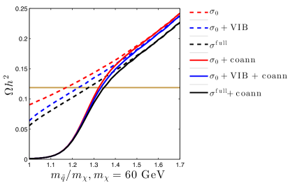
Figure 11: Comparison of the resulting $\Omega h^{2}$ when excluding/ including co-annihilations and excluding/including QCD corrections. For this plot, we again assume the neutralino to be a pure Bino, but fix its mass to $m_{\chi}=60$ GeV; line styles are the same as in Fig. 10. Both VIB and gluon pair production enhance the tree-level annihilation rate significantly, the latter being less suppressed by higher squark masses, but this hardly affects the relic density when taking into account co-annihilations.

From the above discussion we conclude that, for Bino-like neutralinos lighter than the top quark the relic density (considering only annihilations) can be visibly decreased by including gluon VIB in the total annihilation rate – but this effect is inevitably washed out due to the unsuppressed co-annihilations, apart from a small squark mass window around $m_{\tilde{q}}\sim 1.4\,m_{\chi}$. Near top-threshold we see a significant decrease in the relic density due to the virtual loop corrections, $\sigma_{\textrm{tot}}^{\textrm{simp}}$, an effect which is independent of both co-annihilations and VIB. It is worth noting that the above analysis considered the most optimal situation in terms of maximizing the effect of VIB corrections on the relic density. Opening up further channels, e.g. by decreasing any of the other sparticle masses or by allowing small Wino or Higgsino contributions to the neutralino composition, would further decrease the relative contribution from the quark final states and thus the effect of QCD corrections. For example, setting all sfermion masses to be equal would shift the annihilation lines below the top threshold in Fig. 10 by about $m_{\chi}\to 1.8\,m_{\chi}$ due to the different couplings (hypercharges) of squarks and sleptons to a Bino; this is sufficient to completely hide even the small VIB effects one could potentially see in this region of parameter space (c.f. the $m_{\chi}\sim 60$ GeV region in Fig. 12).

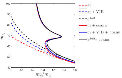
Figure 12: The squark to neutralino mass ratio $m_{\tilde{q}}/m_{\chi}$ that results in $\Omega h^{2}\sim 0.12$, for a given neutralino mass $m_{\chi}$, when assuming a pure Bino annihilating only into quarks. Line styles are again the same as in Fig. 10. Considering only annihilations, VIB corrections have a larger impact on the relic density than gluon pair production for $m_{\tilde{q}}\lesssim 1.2\,m_{\chi}$. In this range, however, the most important contribution comes from the co-annihilations $\chi\tilde{q}_{i}\rightarrow W^{\pm}q_{j}$, $q_{i}g$ and $\tilde{q}_{i}\tilde{q}_{i}^{*}\rightarrow gg$. The peak centered at $m_{\chi}\sim 70$ GeV is due to the resonant top production in the process, $\chi\tilde{t}\rightarrow t^{*}\rightarrow W^{\pm}b$. For lower neutralino masses, both VIB and gluon pair production have a visible, if small, impact on the relic density.

Let us use the remainder of this Section to put these general findings in the context of previous work and concrete scenarios. The impact of QCD corrections to neutralino annihilation on the relic density has been studied by various authors Flores et al. (1989); Drees et al. (1994); Freitas (2007); Herrmann and Klasen (2007); Herrmann et al. (2009a, b); Kovarik and Herrmann (2010); Boudjema et al. (2011); Chatterjee et al. (2012). An extensive study for annihilation into quark final states including all diagrams at $\mathcal{O}(\alpha_{s})$, in particular, was performed by Herrmann et al. Herrmann and Klasen (2007). Here, the focus was on models with neutralinos close to the top threshold where, as noted above, the dominant correction is due to virtual loop corrections. A detailed comparison between our simplified approach and theirs is provided in Appendix A.4.

As also discussed above, coannihilations can increase the total annihilation rate significantly and thereby open up new regions of parameter space for SUSY models for which the relic density otherwise would be too large. Models with squark masses close to the neutralino mass, in particular, can be realized in many extensions of SUSY. For example in cMSSM models, squarks become light when the sfermion mass $m_{1/2}$, is lighter than the common gaugino mass $m_{0}$ and the CP-odd Higgs $A$ is very heavy, $m_{A}\gg m_{\chi}$, which increases the squark mixing Martin (2010). We can further increase the parameter space for such coannihilation scenarios if we consider less constrained models. For example Ref. Herrmann and Klasen (2007) uses non-universal Higgs and gaugino mass models. Another way is to specify the parameters at a lower energy scale (pMSSM models) with the $U(1)$ gaugino mass parameter close to the squark mass, i.e. $M_{1}\lesssim m_{\tilde{q}}$.

Due to experimental and phenomenological constraints, typically only co-annihilation with top squarks is allowed for the most constrained models and thus is of particular interest (for a detailed discussion see Le Boulc’ H (2013)). The stop coannihilation strip in the cMSSM, for example, has been studied in much detail by many authors Boehm et al. (2000b); Ellis et al. (2003); Bednyakov et al. (2002); Santoso (2003); Baer et al. (2002); Edsjo et al. (2003); Ajaib et al. (2012); Diaz-Cruz et al. (2007); Huitu et al. (2011); Ellis et al. (2014); Ibarra et al. (2015), with new limits resulting in particular after the discovery Aad et al. (2012); Chatrchyan et al. (2012) of the Higgs boson. It extends up to neutralino masses of $m_{\chi}\sim 6500$ GeV Ellis et al. (2014), and is as already mentioned realized for very large values of $m_{A}$ (increasing this parameter even further would lead to $m_{\tilde{t}}<m_{\chi}$, rendering the model unphysical). For such large neutralino masses, VIB processes start to dominate neutralino annihilation; in agreement with our previous estimate, we find that $\tilde{\sigma}_{\overline{t}tg}$ becomes equal to $\sigma_{\overline{t}t}$ at around $m_{\chi}\sim 2$ TeV. As indicated by the name, however, the by far largest contribution to the total effective annihilation rate in these scenarios comes from co-annihilations, through $\tilde{t}\chi\rightarrow tg$ and $\tilde{t}\tilde{t}\rightarrow gg$, rather than from annihilation processes Balazs et al. (2004); Freitas (2007). Due to the colored initial states, these and other co-annihilation processes receive sizable QCD corrections; those have been studied in some detail Harz et al. (2013a); Harz (2013); Harz et al. (2013b, 2015a, 2015b) and been found to affect the relic density at a level that exceeds the experimental uncertainty.

Concerning 1st and 2nd generation squarks, both ATLAS Aad et al. (2014, 2015c) and CMS Chatrchyan et al. (2014) report a mass limit of about 850 GeV from generic squark searches, i.e. following a simplified model approach, when assuming all eight squarks to be degenerate in mass; if all but one of these squarks is in the TeV range, the mass limit on the lightest squark is only about 450 GeV. As mentioned earlier, however, these limits do not apply for squarks highly degenerate in mass with the neutralino; mass differences below  20 GeV Chatrchyan et al. (2014) or a few GeV Aad et al. (2015c) remain generally unconstrained. In particular for neutralino and squark masses around roughly 100 GeV, this leaves an intriguing unconstrained window Aad et al. (2014) with interesting model-building options in non-minimal SUSY scenarios. As discussed in Section III, the large VIB contributions in such scenarios become a powerful probe for indirect DM searches. The relic density, on the other hand, is mostly set by co-annihilations and thus not noticeably affected by this kind of QCD corrections.

V Conclusions

Cosmological and astrophysical measurements have reached an impressive level of precision in recent years, calling for a match in terms of equally precise theoretical predictions. With this in mind, we have presented a comprehensive study of the impact of QCD radiative corrections to DM annihilations, focussing on supersymmetric neutralinos.

We find that QCD corrections can indeed very strongly affect the interpretation of indirect DM searches, due to two unrelated effects: i) an enhancement of the helicity-suppressed tree-level cross section by a factor of about $(\alpha_{\mathrm{s}}/\pi)(m_{\chi}/m_{q})^{2}$, in the limit of vanishing relative velocity, and ii) a significant change in the spectrum of the messengers of indirect detection, like gamma rays and cosmic-ray antiprotons (see Figs. 8 and 9). While briefly mentioned in Ref. Asano et al. (2012), in particular the second point has never been addressed in detail before. We also provided updated antiproton limits on DM annihilating into quarks (Fig. 7), and pointed out that the large enhancements of the annihilation rate just mentioned makes indirect searches complementary to a blind spot of collider searches for new physics, namely scenarios where the squarks are almost identical in mass to the DM particle. The impact of the QCD corrections to neutralino annihilation studied here on the relic density, on the other hand, is much smaller because co-annihilations typically dominate. Still, in certain parameter regions these corrections can clearly affect the relic density beyond the level of precision set by current observations (see, e.g., Figs. 10 and 12).

Maybe most importantly, we have presented a fast and efficient way of numerically implementing leading QCD corrections. This method fully captures the above mentioned effects and is in principal extendable in a straight-forward way also to non-supersymmetric models. In particular, we have modelled the annihilating neutralino pair as a decaying pseudoscalar with additional dimension-5 and 6 operators – see Eqs. (10, 20) and the discussion in Appendix A – and approximated the resulting cosmic-ray spectra for a given model as a simple interpolation between the possible extreme cases, see Eqs. (3, 4) and the discussion in Appendix B. We also corrected the effective way in which most current computer codes, like DarkSUSY Gondolo et al. (2004); *dsweb or micrOMEGAs Belanger et al. (2014), handle QCD corrections to the decay of neutralinos (see the discussion in Appendix A.3). This makes both calculations of the relic density and present annihilation rates more reliable, in particular for light quark final states.

Our implementation allows to take into account the leading effects of QCD corrections, especially for indirect DM searches, without the need for numerically expensive full one-loop evaluations or extensive runs of event generators. This leads to a significant gain in performance, which is highly attractive for global scans of high-dimensional parameter spaces, where too time-consuming calculations of relevant observables typically constitute a serious bottleneck. The traditional standard example for the latter are relic density calculations that fully take into account co-annihilations; the most important example in the context of indirect detection, on the other hand, is given by the highly model-dependent cosmic-ray spectra that result when taking into account radiative corrections (see also Ref. Bringmann and Calore (2014); Bringmann et al. (2015)). In this sense, our approach is therefore complementary to that of packages like DM@NLO dmn which aim at full NLO calculations, and hence even higher precision (unless the leading-log resummation that we take fully into account dominates), at the expense of the time required to compute observables for a given model. Another advantage of our method is that we provide the annihilation cross section directly in the limit of vanishing relative velocity, which in most cases is the relevant quantity for indirect DM searches but which presently cannot be provided by DM@NLO. All necessary numerical routines will be included in the next public release of DarkSUSY.

Appendix A Effective Treatment of Neutralino Annihilation

The full calculation of the NLO neutralino cross section can be computationally time consuming, though can be simplified substantially by taking advantage of the majorana nature of the dark matter pair: for small relative velocities, we can approximate the annihilating neutralino pair as the effective decay of a pseudo scalar boson. In Section A.1 we discuss this simplified model and describe its implementation. In Sections A.2 and A.3 we perform the calculation of decays within the simplified model at next to leading order in $\alpha_{s}$, while keeping the full expressions for gluon IB, and finally in Section A.4 we discuss the error associated with using this paradigm to describe neutralino annihilation.

A.1 Approximating Annihilation as Pseudo-Scalar Decay

As discussed briefly in Section II, a pair of non-relativistic Majorana neutralinos transforms to an excellent approximation as a pseudo-scalar under Lorentz transformations. Practically this means that the initial state fermion bi-linear in the amplitude can be replaced with the $s$-wave projector $P_{S_{0}}=\frac{\gamma^{5}}{\sqrt{2}}(m_{\chi}-\not{p}/2)$, where $m_{\chi}$ is the neutralino mass and $p$ is the total momentum of the system (see, e.g., Ref. Calore (2013)). Assuming no $CP$-violating interactions, the tree-level amplitude for $\chi\chi\rightarrow\bar{q}q$ thus reduces to the same form as that of a decaying pseudo scalar $\phi$ with mass $M=2m_{\chi}$, up to a conventional constant normalization factor $A$ of mass dimension one, with an interaction Lagrangian given by

$$\mathcal{L}_{\textrm{int}}^{\mathrm{simp}}=-g_{p}\phi\bar{q}i\gamma^{5}q-\frac{1}{\Lambda_{a}}\partial_{\mu}\phi\bar{q}\gamma^{\mu}\gamma^{5}q\,.$$ (10)

Here, $g_{p}$ is an effective pseudo scalar coupling, and $\Lambda_{a}$ is an effective axial-vector coupling with mass dimension one. This leads to a squared matrix element of

$$\left|\mathcal{M}\right|^{2}=2M^{2}\left(g_{p}+\frac{2m_{q}}{\Lambda_{a}}\right)^{2}\,.$$ (11)

The same result, divided by $A^{2}$, is obtained in the case of annihilation, implying the following relation between the total quark production rate in this simplified model $\Gamma_{0}^{\textrm{simp}}$ and the total tree level neutralino cross section $\sigma_{0}^{\textrm{full}}$:

$$\Gamma_{0}^{\textrm{simp}}=A^{2}m_{\chi}\sigma_{0}^{\textrm{full}}v\,.$$ (12)

From here on the superscript ‘simp’ stands for calculations done in the simplified model and implicitly includes contributions from all operators in Eq. (10).

In the interest of relating the full cross section $\sigma_{\textrm{tot}}^{\textrm{full}}$ at NLO to the decay rate of our simplified model, we will now generalize Eq. (12) to an arbitrary sub-process $X$, and define an annihilation rate $\sigma^{\textrm{simp}}_{X}v$ by the corresponding decay rate in the simplified model,

$$\sigma^{\textrm{simp}}_{X}v\equiv\dfrac{\Gamma^{\textrm{simp}}_{X}}{A^{2}m_{\chi}}.$$ (13)

At tree level ($X=0$), we thus have $\sigma^{\textrm{simp}}_{0}=\sigma^{\textrm{full}}_{0}$ by construction, but in general one expects $\sigma^{\textrm{simp}}_{X}\neq\sigma^{\textrm{full}}_{X}$ (note, however, that the dependence of $\sigma^{\textrm{simp}}$ on the conventional factor $A$ always cancels). In general $\sigma^{\textrm{simp}}_{X}$ does thus not constitute a physical cross section, but is simply a useful device for comparing the simplified model to the full neutralino cross section.

Figure 13: Diagrams contributing to pseudo scalar decay up to $\mathcal{O}(\alpha_{s})$: (a) Tree level decay, (b) FSR off of $q$, (c) FSR off of $\bar{q}$, (d) 1-loop vertex correction, (e) counterterm diagram.

Henceforth we will denote vertex corrections by $X=V$, counter terms by $X=C$ and gluon internal bremsstrahlung by $X=B$. The diagrams for the contributing processes in the simplified model are pictured in Fig. 13: the cross section up to order $\alpha_{s}$ is given by the sum of tree level and bremsstrahlung cross sections, $\sigma_{0}^{\textrm{simp}}$ and $\sigma_{B}^{\textrm{simp}}$, plus the interference between tree level and vertex correction ($\sigma_{V}^{\textrm{simp}}$) as well as counter terms ($\sigma_{C}^{\textrm{simp}}$). For the full model, we thus have

$$\sigma_{\textrm{tot}}^{\textrm{full}} = \sigma_{0}^{\textrm{full}}+\sigma_{B}^{\textrm{full}}+\sigma_{V}^{\textrm{full}}+\sigma_{C}^{\textrm{full}}+\sigma_{\star}^{\textrm{full}}$$ (14)

$$= \sigma_{\textrm{tot}}^{\textrm{simp}}+(\sigma_{\textrm{tot}}^{\textrm{full}}-\sigma_{\textrm{tot}}^{\textrm{simp}})$$

$$= \sigma_{\textrm{tot}}^{\textrm{simp}}+\tilde{\sigma}_{\bar{q}qg}+\sigma_{\textrm{Error}}$$

where $\sigma^{\textrm{full}}_{\star}$ denotes interference terms between the tree-level result and additional diagrams not present in the simplified model, and

$$\sigma_{\textrm{Error}} \equiv (\sigma_{V}^{\textrm{full}}-\sigma_{V}^{\textrm{simp}})+(\sigma_{C}^{\textrm{full}}-\sigma_{C}^{\textrm{simp}})+\sigma_{\star}^{\textrm{full}}.$$ (15)

In the final step, we also have introduced the FSR subtracted 3-body cross section 

$$\tilde{\sigma}_{\bar{q}qg}\equiv(\sigma_{B}^{\textrm{full}}-\sigma_{B}^{\textrm{simp}})\,.$$ (16)

The calculation of the full NLO cross section can thus be broken up into two pieces, the model independent $\sigma_{\textrm{tot}}^{\textrm{simp}}$, which we calculate analytically in Section A.3, and the just introduced quantity $\tilde{\sigma}_{\bar{q}qg}$ which, as we discuss next, contains potentially large corrections due to lifting the helicity suppression of $\sigma^{\textrm{full}}_{0}$. The error in using the simplified model, $\sigma_{\textrm{Error}}$, is in general model dependent but expected to be small, and will be discussed further in Section A.4.

A.2 Internal bremsstrahlung

In the simplified model, internal bremsstrahlung of a gluon proceeds via the final state radiation diagrams b) and c) depicted in Fig. 13. For this process, we calculate the double differential rate as

$$\frac{d^{2}\sigma^{\textrm{simp}}_{B}}{dx_{g}dx_{q}} = \frac{\alpha_{s}C_{F}\sigma^{\textrm{simp}}_{0}}{4\pi\sqrt{1-\mu_{q}}}\times$$

$$\frac{\mu_{q}x_{g}^{2}+2((1-x_{g})^{2}+1)(1-x_{g})(1-x_{g}-x_{q})}{(1-x_{q})^{2}(1-x_{g}-x_{q})^{2}}\,,$$

which once integrated over the quark energy becomes

$$\frac{d\sigma^{\textrm{simp}}_{B}}{dx_{g}} = \frac{2\alpha_{s}C_{F}\sigma^{\textrm{simp}}_{0}}{\pi x_{g}\sqrt{1-\mu_{q}}}\Bigg{[}\left(1-\mu_{q}\right)\sqrt{(1-x_{g})(1-x_{g}-\mu_{q})}$$

$$-\left(1+(1-x_{g})^{2}-\mu_{q}\right)\tanh^{-1}\!\!\sqrt{1-\frac{\mu_{q}}{1-x_{g}}}\Bigg{]},$$

where $x_{g}\equiv E_{g}/m_{\chi}$ and $\mu_{q}\equiv m_{q}^{2}/m_{\chi}^{2}$, and $C_{F}=4/3$ is the $SU(3)$ Casimir operator associated to gluon emission from quarks. In the limit of small quark masses, $\mu_{q}\ll 1$, this reduces as expected to the well-known Weizsäcker-Williams expression Bergström et al. (2005); Birkedal et al. (2005)

$$\frac{d\sigma^{\textrm{simp}}_{B}}{dx_{g}}=\sigma^{\textrm{simp}}_{0}\frac{\alpha_{s}C_{F}}{\pi x_{g}}\left[1+(1-x_{g})^{2}\right]\log\frac{4(1-x_{g})}{\mu_{q}}\,.$$ (19)

Note that the above result is model-independent in the sense that the parameters of the simplified-model Lagrangian (10) do not explicitly enter in this expression. This changes when considering the full model because of VIB contributions, which can be traced back to the emission of gluons from $t$-channel squarks. In the language of the simplified model pseudoscalar $\phi$, these processes generate three ‘anomalous’ types of 4-point interactions given by dimension-5 and 6 operators, respectively:

$$\mathcal{L}^{\mathrm{simp}}_{\mathrm{VIB}} = -\frac{1}{\Lambda_{p4}}\phi t_{a}A^{\mu}_{a}\bar{q}i\gamma^{5}\overset{\leftrightarrow}{\partial_{\mu}}q-\frac{1}{\Lambda_{a4}^{2}}(\partial_{\mu}\phi)t_{a}A^{\nu}_{a}\bar{q}\overset{\leftrightarrow}{\partial_{\nu}}\gamma^{\mu}\gamma^{5}q$$ (20)

$$-\frac{1}{\Lambda_{v4}^{2}}(\partial_{\mu}\phi)t_{a}A^{\nu}_{a}\bar{q}\overset{\leftrightarrow}{\partial_{\nu}}\gamma^{\mu}q\,,$$

where $t_{a}$ are the $SU(3)$ generators and $A^{\mu}_{a}$ the gluon fields. These operators thus arise in the zero velocity and quark-mass limit of the full theory, but are absent even at higher orders in the theory described by Eq. (10) (recall that $g_{p}\propto m_{q}$); hence, they contribute to $\tilde{\sigma}_{\bar{q}qg}$ in Eq. (16), but not to $\sigma^{\mathrm{simp}}_{\mathrm{tot}}$. This is a simple way of seeing how the helicity suppression of $\phi\to\bar{q}q$ can technically be lifted by gluon VIB.

To obtain the IB cross section in the full theory, which strongly depends on the choice of SUSY model, we use Eq. (2) to rescale the analytical solutions derived in Ref. Bringmann et al. (2008). As required by Kinoshita’s and Bloch’s theorems Kinoshita (1962); Bloch and Nordsieck (1937), the difference $(d\sigma_{B}^{\textrm{full}}/dx-d\sigma_{B}^{\textrm{simp}}/dx)$ is no longer IR divergent, nor divergent in the $\mu_{q}\to 0$ limit (see also the discussion in Appendix B). We can therefore integrate it numerically to obtain the second term in our final result for the full cross section at leading order in $\alpha_{s}$, Eq. (14).

A.3 Pseudo-Scalar Decay at NLO

Figure 14: 1-loop contribution to the quark self energy $\Sigma$.

The total NLO rate of quark production in the simplified model has contributions from the two operators in Eq. (10), as well as from the gluon coupling to quarks. Being very similar to the decay of the scalar and pseudo scalar Higgs’, we follow very closely the calculations of Refs. Braaten and Leveille (1980); Drees and Hikasa (1990a). We thus have to consider the renormalized Lagrangian

$$\mathcal{L}=\bar{q}(i\not{D}-m_{q})q-ig_{p}(1+\delta_{p})\phi\bar{q}\gamma^{5}q-\frac{1+\delta_{a}}{\Lambda}\partial_{\mu}\phi\bar{q}\gamma^{\mu}\gamma^{5}q\,.$$ (21)

The counter terms $\delta_{p}$ and $\delta_{a}$ cancel the ultraviolet divergences from the vertex corrections in Fig. 13 (d) to pseudo-scalar and axial vector decays respectively. In the on shell renormalization scheme, they are given by

$$\delta_{p} = \delta_{Z}-\delta m/m_{q}+\delta^{5}_{p},$$

$$\delta_{a} = \delta_{Z}+\delta^{5}_{a},$$ (22)

where $m_{q}$ is the quark mass at the weak scale, and $\delta_{Z}$ and $\delta_{m}$ are the quark field re-scaling counterterm and mass rescaling respectively. The terms $\delta^{5}_{p/a}$ renormalize the axial anomaly, that is, they take account of the fact that $\{\gamma^{5},\gamma^{\mu}\}\neq 0$ in $D$ dimensions, and are required to maintain gauge invariance during the renormalization procedure Larin (1993):

$$\delta^{5}_{p} = -\frac{\alpha_{s}}{4\pi}8C_{F}\,,$$

$$\delta^{5}_{a} = -\frac{\alpha_{s}}{4\pi}4C_{F}\,.$$ (23)

Note that the axial vector coupling is non-renormalizable, so the counterterm $\delta_{a}$ is an effective counterterm to cancel the divergence from the effective coupling; the Ward identity will ensure that a similar term proportional to the field re-scaling will cancel the divergences in the full theory Berends et al. (1973, 1983); Akhundov et al. (1985); Peskin and Schroeder (1995). $\delta m$ and $\delta_{Z}$ are derived from the quark self-energy, Fig. 14, and are given by

$$\frac{\delta m}{m_{q}} = \frac{\alpha_{s}C_{F}}{4\pi}\left[3\Gamma(\epsilon)-3\log\left(\frac{\mu_{q}}{4\pi}\right)+4\right],$$ (24)

$$\delta_{Z} \equiv Z_{2}-1$$

$$\simeq \frac{\alpha_{s}C_{F}}{4\pi}\left[-\Gamma(\epsilon)+3\log\left(\frac{\mu_{q}}{4\pi}\right)-\log(\mu_{g})-4\right],$$

where $D\equiv 4-2\epsilon$ to dimensionally regulate the UV divergence, and $\mu_{g}$ is a fictitious gluon mass (in units of $m_{\chi}^{2}$) introduced to regulate the infrared (IR) divergence. We have omitted propagator counter terms in Eq. (21), as their relevance only comes in at $\mathcal{O}(\alpha_{s}^{2})$.

Real gluon emission from final state quark legs has already been discussed above, and is described by Eq. (A.2). The IR divergence of $\sigma_{B}^{\textrm{simp}}$ is canceled by a corresponding divergence in $\sigma_{V}^{\textrm{simp}}+\sigma_{C}^{\textrm{simp}}$. Adding all processes discussed above leads to the total annihilation rate for the simplified model,

$$\sigma_{\textrm{tot}}^{\textrm{simp}}=\sigma_{0}^{\textrm{simp}}+\sigma_{B}^{\textrm{simp}}+\sigma_{V}^{\textrm{simp}}+\sigma_{C}^{\textrm{simp}}.$$ (25)

In a different context, this has earlier been calculated by Drees and Hikasa Drees and Hikasa (1990a)

$$\frac{\sigma_{\textrm{tot}}^{\textrm{simp}}}{\sigma_{\textrm{0}}^{\textrm{simp}}} = 1+\dfrac{C_{F}\alpha_{s}}{\pi}\Bigg{[}\frac{1+\beta_{0}^{2}}{\beta_{0}}\left(4\textrm{Li}_{2}\left(\dfrac{1-\beta_{0}}{1+\beta_{0}}\right)+2\textrm{Li}_{2}\left(-\dfrac{1-\beta_{0}}{1+\beta_{0}}\right)-3\log\dfrac{2}{1+\beta_{0}}\log\dfrac{1+\beta_{0}}{1-\beta_{0}}-2\log\beta_{0}\log\dfrac{1+\beta_{0}}{1-\beta_{0}}\right)$$ (26)

$$\phantom{1+\dfrac{C_{F}\alpha_{s}}{\pi}\Bigg{[}}-3\log\dfrac{4}{1-\beta_{0}^{2}}-4\log\beta_{0}+\dfrac{1}{16\beta_{0}}(19+2\beta_{0}^{2}+3\beta_{0}^{4})\log\dfrac{1+\beta_{0}}{1-\beta_{0}}+\dfrac{3}{8}(7-\beta_{0}^{2})\Bigg{]},$$

where $\beta_{0}\equiv\sqrt{1-\mu_{q}}$. We have verified that in the rest frame of the $\phi$ Eq. (26) is true for both pseudo scalar and axial vector interactions. As Eq. (26) approaches the quark threshold, $\beta_{0}\to 0$, it diverges. This is a consequence of the colour Coulomb interaction, and signifies the formation of bound states Drees and Hikasa (1990b); Reinders et al. (1980). Very close to the threshold the above expression thus needs to be corrected which however is outside the scope of this work.

In the limit $\mu_{q}\to 0$ of small quark masses, relevant for models with large VIB enhancements, this reduces to

$$\sigma_{\textrm{tot}}^{\textrm{simp}}\simeq\sigma_{0}^{\textrm{simp}}\left[1+\frac{3\alpha_{s}C_{F}}{4\pi}\left(3+2\log\frac{\mu_{q}}{4}\right)\right],$$ (27)

a result which we derived independently and confirm. As required by Kinoshita’s theorem Kinoshita (1962) the unrenormalized rate must be free of mass divergences, thus the logarithmic divergence in Eq. (27) comes from the counter terms in Eq. (21). For very small values of $\mu_{q}$, this divergence indicates a breakdown in the reliability of the $\mathcal{O}(\alpha_{s})$ calculation, and we are required to re-sum the leading log contributions to all orders in $\alpha_{s}$. This results in replacing the leading log term in the above expression as Braaten and Leveille (1980); Drees and Hikasa (1990a)

$$\frac{6\alpha_{s}C_{F}}{\pi}\log\frac{\mu_{q}}{4}\rightarrow\left(\frac{\mbox{ln}(4m_{q}^{2}/\Lambda_{QCD}^{2})}{\mbox{ln}(s/\Lambda_{QCD}^{2})}\right)^{\frac{24}{33-2N_{f}}}\,,$$ (28)

where $N_{f}$ is the number of accessible quark flavours, and $\Lambda_{QCD}$ is the QCD scale. This can be simplified further using the identity for the running quark mass, defined in the MS scheme

$$\frac{\overline{m}(\mu)}{\overline{m}(\mu_{0})}=\left[\frac{\alpha_{s}(\mu)}{\alpha_{s}(\mu_{0})}\right]^{\frac{2}{\pi b}}=\left[\frac{\mbox{ln}(\mu_{0}/\Lambda_{QCD})}{\mbox{ln}(\mu/\Lambda_{QCD})}\right]^{\frac{2}{\pi b}},$$ (29)

where $b=(33-2N_{f})/(6\pi)$, and $\alpha_{s}(\mu)^{-1}\simeq b\,\mbox{ln}(\sqrt{s}/\Lambda_{QCD})$ in the limit $\sqrt{s}\gg\Lambda_{QCD}$. Noting that at zeroth order in $\alpha_{\mathrm{s}}$ the physical (pole) mass is equal to $m_{q}=\overline{m}(2m_{q})$, we can see clearly that the effect of the re-summation of leading logarithms coming from the renormalization procedure, equates to replacing $g_{p}$ with a running Yukawa coupling. For consistency we also make this replacement in the tree level amplitude leaving us with a result that is both valid in the $\mu\to 0$ limit and interpolates with the full one-loop result (25) Drees and Hikasa (1990a)

$$\frac{\sigma_{\textrm{tot}}^{\textrm{simp}}}{\sigma_{0}^{\textrm{simp}}}\simeq\frac{\overline{m}^{2}(\sqrt{s})}{\overline{m}^{2}(2m_{q})}\left[1+\frac{9\alpha_{s}C_{F}}{4\pi}\right].$$ (30)

This expression constitutes the main result of Appendix A.3, so let us pause a moment to discuss it in more detail. For pseudo-scalar processes the interpretation of this result is clear, we have simply re-derived the running of the Yukawa interactions as in Braaten and Leveille (1980); Drees and Hikasa (1990a) The interpretation for the contribution from the axial vector interaction in Eq. (10) is a little more subtle, but essentially boils down to the observation that only the time-like part of the axial vector coupling contributes to the decay of a pseudo scalar (because $p^{\mu}=(\sqrt{s},\mathbf{0})$ in the rest frame of $\phi$); as this component has exactly the same transformation properties under rotations and mirror operations, we should expect to find the same results in both cases. It is also worth to reflect about the overall normalization of Eq. (30), which fixes the renormalization fix point for the running of the quark masses such that the tree-level result is recovered at threshold, i.e. for $\sqrt{s}=2m_{q}$. This appears – in hindsight, recall that we made no corresponding assumption during our derivation – to be the only possible energy scale at which one could sensibly require this to happen, simply because it is the only one that is available: the masses of virtual particles (such as the pseudoscalar $A$) only appear in a subset of relevant diagrams; and the neutralino pair is in some diagrams not even connected to the vertex to which we have calculated QCD corrections, hence the pseudoscalar mass $M=\sqrt{s}\simeq 2m_{\chi}$ is not a good alternative either. Let us stress that this situation is intrinsically different to the running of the Yukawa coupling $y$ of the SM Higgs boson to fermions. In that case, a well-motivated (and in fact standard) renormalization fixpoint would be to require that the Higgs decay at rest corresponds to the one expected at tree level, which amounts to take into account the running by replacing $y_{q}\sim m_{q}$ with $y_{q}\sim\overline{m}(\sqrt{s})/\overline{m}(m_{h})$.

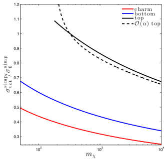
Figure 15: Ratio of the total and tree level cross sections in the simplified model for $\bar{c}c$ (red), $\bar{b}b$ (blue), $\bar{t}t$ (black) quark final states (solid lines). For $\bar{t}t$, also NLO results are shown (dashed). All ratios use running $\alpha_{s}(2m_{\chi})$.

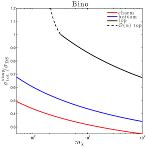
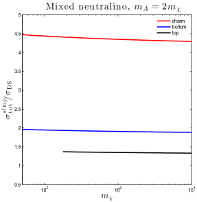
Figure 16: Ratio of our result for ${\sigma_{\textrm{tot}}^{\textrm{simp}}}$ and the annihilation cross section $\sigma^{\mathrm{DS}}$ as implemented in DarkSUSY 5.1.2. The various lines correspond to $\bar{c}c$ (red), $\bar{b}b$ (blue), $\bar{t}t$ (black) final states. Left panel: case of a pure Bino. Right panel: case of a mixed neutralino where annihilation via an $s$-channel pseudoscalar Higgs dominates. See text for a detailed discussion.

The ratio (30) of the QCD-corrected over tree-level cross section in the simplified model is shown in Fig. 15 for $c$, $t$ and $b$ quarks, where we have used the 4-loop results from Refs. Chetyrkin and Kühn (1990); Chetyrkin et al. (2000) for the running MS quark masses (as implemented in DarkSUSY). The figure illustrates that the total cross section is significantly suppressed by QCD corrections for all quark final states across most of the parameter space, with the exception of top final states in the region close to the top threshold (though in the presence of substantial VIB contributions, not included in ${\sigma_{\textrm{tot}}^{\textrm{simp}}}$, the cross section will of course instead be enhanced, by a factor proportional to $m_{\chi}^{2}$). For top final states, we show for comparison also the NLO result of Eq. (26), which should be used for neutralino masses not much greater than the final state quark mass because the re-summed expression (30) is only valid for $m_{q}\gg m_{\chi}$. In practice, we implement a somewhat arbitrary ratio of $m_{\chi}/m_{q}=1.85$ to divide between those two regimes (this is where the two lines in the figure cross).

We conclude this Section by comparing our results with the way QCD corrections are currently implemented in DarkSUSY 5.1.2, which essentially amounts to including the effect of running quark masses solely in the Yukawa couplings that appear at tree-level (noting that micrOMEGAs Belanger et al. (2014) uses a very similar implementation). As discussed above, this incorrectly neglects the contribution from diagrams where the SM model Yukawa couplings do not enter explicitly, but which give an identical description in terms of our effective pseudo-scalar model. To illustrate the size of this effect, we show in Fig. 16 the ratio of our improved result for $\sigma_{\textrm{tot}}^{\textrm{simp}}$ and the cross section $\sigma^{\mathrm{DS}}$ used in DarkSUSY for two specific situations: i) a pure Bino with the same characteristics as used in Section IV (left panel) and ii) a mixed neutralino in the ‘Higgs funnel’ region with $m_{A}=2m_{\chi}$ (right panel), chosen such that the annihilation rate is by far dominated by the exchange of a pseudoscalar Higgs in the $s$-channel. In the Bino case, the couplings that appear in annihilation diagrams have only subdominant Yukawa contributions (because we set the squark mixing to zero). Hence, $\sigma^{\mathrm{DS}}$ is as expected identical to the tree-level result, implying that the ratio $\sigma_{\textrm{tot}}^{\textrm{simp}}/\sigma^{\mathrm{DS}}$ is simply given by Eqs. (26, 30) and hence Fig. 16. For the case of a pseudoscalar mediator in the $s$-channel, on the other hand, the origin of the leading correction factor in Eq. (30) comes exclusively from the Yukawa coupling between $A$ and final quark pair, and we might therefore expect exact agreement of our result with the DarkSUSY implementation. As visible in the figure, however, this is not the case. The reason for this discrepancy is that DarkSUSY 5.1.2 implements the Yukawa running independently of the process under consideration by replacing $m_{q}\to\overline{m}(2m_{\chi})$ (as do many other numerical codes, including micrOMEGAs and, to some extent, DM@NLO). As discussed at length above, however, this corresponds to an unphysical renormalization condition for the specific process we are interested in here (i.e. the decay of an effective pseudoscalar particle with mass $M=\sqrt{s}$). Indeed, when artificially replacing ${\overline{m}^{2}(2m_{\chi})}/{\overline{m}^{2}(2m_{q})}\to{\overline{m}^{2}(2m_{\chi})}/m_{q}^{2}$ in Eq. (30), we find exact agreement as expected – up to the term $9C_{F}\alpha_{s}/4\pi$ which is not included in DarkSUSY. Numerically, the discrepancy between those two prescriptions is largest for light quarks.

As just illustrated, our corrected version of $\sigma_{\textrm{tot}}^{\textrm{simp}}$ can significantly affect predictions for the annihilation rate of a given SUSY model. We numerically implement it into DarkSUSY, alongside the difference $(\sigma_{B}^{\textrm{full}}-\sigma_{B}^{\textrm{simp}})$, thereby making both calculations of the relic density and present annihilation rates with this widely used tool significantly more reliable. The accuracy of neglecting the remaining term in Eq. (14), $\sigma_{\textrm{Error}}$, will be discussed below.

A.4 Expected Error

The accuracy in treating dark matter annihilation as an effective decay at NLO is limited by the model dependent contribution $\sigma_{\textrm{Error}}$. As illustrated by Eq. (15), this term has two contributions, the first is from the difference between the full theory and the simplified model, taking into account only final state gluon exchange graphs at NLO and appropriate counterterms. The second type of error, $\sigma_{\star}$, comes from neglected Feynman diagrams at the one loop level. Though the full calculation of these contributions is beyond the scope of this work, we can make an educated guess about their importance.

The $s$-channel $Z$ and $A$ mediated contributions to Fig. 4 have an identical vertex topology to axial vector and pseudo scalar decay processes, implying that for these diagrams the cancellations in Eq. (15) are exact up to all orders in $\alpha_{s}$. This is not the case for $t$-channel squark exchange as the $t$-channel propagator is a function of the off-shell gluon momentum. Using simple power counting arguments, however, it is clear that the $t$-channel contribution to Fig. 4 (a) is UV finite, negating the need for a counterterm for this diagram. However, to maintain gauge invariance we must add to this process $t$-channel graphs with $\mathcal{O}(\alpha_{s})$ corrections to the neutralino-quark-squark vertex, which do indeed contain a UV divergence. As it turns out when neutralino-quark-squark vertex correction graphs are taken into account, the subtraction $(\sigma_{V}^{\textrm{full}}-\sigma_{V}^{\textrm{simp}})$ has no UV divergence, implying that in the term $(\sigma_{C}^{\textrm{full}}-\sigma_{C}^{\textrm{simp}})$ the cancellation of leading mass logarithms must also be exact. Similarly, when we add all $\mathcal{O}(\alpha_{s})$ amplitude contributions including counterterms, we expect all IR divergences to cancel. One therefore expects some model-dependent error to enter in at $\mathcal{O}(\alpha_{s})$, from in-exact $t$-channel cancellations in Eq. (15), but that this error cannot contain large mass logarithms, and is therefore expected to be small compared to Eq. (30) – or the VIB contributions, $\sigma_{B}^{\textrm{full}}-\sigma_{B}^{\textrm{simp}}$, which dominate as several times stressed for $m_{\chi}\gg m_{q}$.

$\sigma_{\star}$ contains loops involving gluinos, squark self energy graphs, and supersymmetric corrections to the quark self energy. While the error from neglecting $\sigma_{\star}$ enters at $\mathcal{O}(\alpha_{s})$ and in general is very model-dependent, we expect it not to be very sizable. The reason is that even though these additional diagrams potentially lead to large mass logarithms containing squark and gluino masses, those are typically not as large as the fully accounted-for logarithms containing quark masses in the $m_{q}\ll 2m_{\chi}$ limit (simply because the mass separation between supersymmetric states typically does not extend over several orders of magnitude). An exception to this general expectation are $b$ quark final states where an extra source of error comes from sbottom-gluino and stop-chargino one-loop contributions to $m_{b}$, which can be substantial for large $\tan\beta$ or large $A_{b}$, and as such need to be re-summed Carena et al. (2000); Guasch et al. (2003); Herrmann and Klasen (2007). The result is a correction to the $b$ mass which leads to an error in the simplified model cross section at zeroth order in $\alpha_{s}$. While these unmodelled contributions to $\sigma_{\textrm{Error}}$ are potentially worrisome, they are all helicity suppressed. Their importance thus diminishes when we consider models with large VIB $(\sigma_{B}^{\textrm{full}}-\sigma_{B}^{\textrm{simp}})$ contributions, the main interest of this work. From this discussion, we generally expect the biggest error in the cross section to come from neutralino annihilation into top quarks, for neutralino masses not too far above threshold.

	$m_{0}[GeV]$	$M_{2}[GeV]$	$A_{0}[GeV]$	$\tan\beta$	sign$(\mu)$	$m_{H_{u}}[GeV]$	$m_{H_{d}}[GeV]$	$m_{\tilde{\chi}_{1}^{0}}$	$m_{\tilde{t}}$	$\Delta_{\textrm{full}}$ dmn (Herrmann et al. (2009a))	$\Delta_{\textrm{simp}}$ [this work]	Diff. [%]
I	500	500	0	10	$+$	1500	1000	207.2	606.4	– (1.22)	1.22	$<$1
II	620	580	0	10	$+$	1020	1020	223.7	923.8	1.32 (1.59)	1.15	-13
III	500	500	-1200	10	$+$	1250	2290	200.7	259.3	1.26 (1.22)	1.25	1

Table 3: mSUGRA models with non-universal Higgs masses considered in Ref. Herrmann et al. (2009a). The quantity $\Delta$ denotes the ratio of QCD-corrected to tree-level annihilation cross section to top quarks in the zero-velocity limit. The values obtained with the current version of DM@NLO dmn were kindly provided by B. Herrmann Herrmann (2015).

	$m_{0}[GeV]$	$M_{2}[GeV]$	$A_{0}[GeV]$	$\tan\beta$	sign$(\mu)$	$\frac{M_{1}}{M_{2}}$	$\frac{M_{3}}{M_{2}}$	$m_{\tilde{\chi}_{1}^{0}}$	$m_{\tilde{t}}$	$\Delta_{\textrm{full}}$ dmn (Herrmann et al. (2009a))	$\Delta_{\textrm{simp}}$ [this work]	Difference [%]
IV	300	700	-350	10	$+$	2/3	1/3	183.4	281.9	1.43 (1.25)	1.49	4
V	1500	600	0	10	$+$	1	4/9	235.6	939.0	1.34 (1.55)	1.12	-16

Table 4: As Table 3, but for models in mSUGRA without gaugino mass unification.

To test the accuracy of our simplified model in this ‘critical regime’, we compared the DarkSUSY result for the total neutralino cross section at NLO ($\sigma_{0}^{\textrm{simp}}$ for ${\chi\chi\rightarrow\bar{t}t\,\&\,\bar{t}tg}$) with the full NLO result Herrmann et al. (2009a); dmn , which makes no simplifying assumptions and includes all $\mathcal{O}(\alpha_{s})$ diagrams. Given differences in the treatment of the running of SUSY parameters, the value of $\sigma_{0}^{\textrm{simp}}$ calculated in DarkSUSY generally does not agree with the corresponding result in Herrmann et al. (2009a) at tree level. Therefore, to get a better representation of the error in our result, we only consider the fractional enhancement $\Delta$ of the zero velocity cross section at NLO over the tree level result. In Tables 3 and 4, we show this quantity for the models explicitly considered in Ref. Herrmann et al. (2009a). Concretely, $\Delta_{\textrm{full}}\equiv{\sigma_{\textrm{tot}}^{\textrm{full}}}/{\sigma_{0}}$ represents the enhancement reported in Herrmann et al. (2009a), updated by using the latest version of DM@NLO dmn , while $\Delta_{\textrm{simp}}\equiv{\sigma_{\textrm{tot}}^{\textrm{simp}}}/{\sigma_{0}}$ represents the enhancement within the simplified model discussed in this work.

From this simple comparison the error in using the simplified model appears to be well below $20\%$ for neutralino masses close to the top threshold. In some cases, like for model I, we find agreement with the full result to excellent precision. This is not altogether surprising given that in this model annihilation at tree level is dominated by $A$ exchange, which only contributes to $\sigma_{\textrm{Error}}$ at NLO through a gluino-squark loop diagram which is expected to be sub-dominant in comparison to the leading contributions. In models II and V annihilation at tree level is dominated by $Z$ exchange. These constitute the worst agreement between the full theory and the simplified model, implying that the $Z$ mediated gluino-squark loop process is important. In models III and IV annihilation at tree level is dominated by $\tilde{q}$ exchange and negative $Z/\tilde{q}$ interference terms. Thus the neglect of mixing terms between tree-level squark exchange and the $Z$ mediated gluino-squark loop is a likely explanation for the – in fact not very sizeable – relative enhancement of the simplified model calculation over the full NLO result from DM@NLO dmn ; Herrmann (2015).

We reiterate that the above comparison has focussed on the most pessimistic case, as we expect the error in using the simplified model to be largest for close-to-threshold annihilation into $\bar{t}t$ pairs (because of the sub-dominance of $\bar{t}tg$ VIB relative to 2-body annihilation in this case). Given the advantages of our approach, in particular in terms of numerical performance, the agreement is thus actually surprisingly good. Let us also stress that the full NLO result Herrmann et al. (2009a) of course does not take into account leading logarithms from higher orders in $\alpha_{\mathrm{s}}$, which need to be re-summed as they increase in importance. Far above threshold, for $m_{\chi}\gg m_{q}$, the result presented in Eq. (30) can thus actually expected to provide a more accurate estimate of the annihilation rate than the full NLO result.

Appendix B Stable particle spectra from neutralino annihilation

In Appendix A we have discussed in some detail how to approximate the full and differential cross section for the annihilation of two neutralinos in the framework of a simplified model that describes the decay of a pseudo scalar. We now turn to the computation of the spectrum of stable particles like photons or antiprotons that result from showering and fragmentation of the $\bar{q}q$ and $\bar{q}qg$ final states, again using the framework of our simplified model. The flux of these stable particles at source, i.e. before propagation in the galactic halo, is conventionally written in the form $d\Phi/dT\propto\sigma_{0}^{\mathrm{full}}dN/dT$. Here, $\sigma_{0}^{\mathrm{full}}=\sigma_{0}^{\mathrm{simp}}$ is the tree-level annihilation cross section into $\bar{q}q$ and $dN/dT$ is the differential number of antiprotons or photons per tree-level annihilation. Following from Eq. (14), it is given by

$$\frac{dN}{dT}=\frac{\sigma_{\textrm{tot}}^{\textrm{simp}}+\sigma_{\textrm{Error}}}{\sigma_{0}^{\mathrm{simp}}}\frac{dN_{\bar{q}q}}{dT}+\frac{\tilde{\sigma}_{\bar{q}qg}}{\sigma_{0}^{\mathrm{simp}}}\frac{d\tilde{N}_{\bar{q}qg}}{dT},$$ (31)

where $\tilde{\sigma}_{\bar{q}qg}\equiv(\sigma_{B}^{\textrm{full}}-\sigma_{B}^{\textrm{simp}})$ and $T$ is the kinetic energy of the stable particle in question. This spectrum is determined by four independent quantities which we will now discuss in more detail.

$\sigma_{\textrm{tot}}^{\textrm{simp}}$ and $\tilde{\sigma}_{\bar{q}qg}$ determine the normalization of the spectrum, and correspond to the simplified model and subtracted IB cross sections defined in Appendix A.1 (recall that we neglect the contribution from $\sigma_{\textrm{Error}}$, see discussion in Appendix A.4). They can be thought of as the normalizations of “2-body” and “3-body” spectra respectively, though in reality the simplified model cross section implicitly includes FSR contributions. Note in particular that using the subtracted IB cross section as a normalization for the 3-body part automatically ensures that there is no double-counting of processes already included in the 2-body part.

The $dN_{\bar{q}q}/dT$ is the differential number of antiprotons or gamma-rays per total annihilation for the simplified model, and is the same as the result obtained by simulation of a 2-body $\bar{q}q$ final state in Pythia, including final state showering and hadronization. Given that the final state $\bar{q}q$ pair is produced back to back, the shape of this spectrum is only a function of $m_{\chi}$ and $m_{q}$. $d\tilde{N}_{\bar{q}qg}/dT$ on the other hand is what we call the subtracted 3-body spectrum. Explicitly it is the differential number of antiprotons/gamma-rays per annihilation $\tilde{\sigma}_{\bar{q}qg}$, obtained after simulations of $\bar{q}qg$ final states in Pythia with a center of momentum energy of $2m_{\chi}$, randomly selecting 3-body kinematical distributions according to the probability distribution

$$\frac{d^{2}\tilde{N}_{\bar{q}qg}}{dx_{g}dx_{q}}\equiv\frac{1}{\tilde{\sigma}_{\bar{q}qg}}\left(\frac{d^{2}\sigma_{B}^{\textrm{full}}}{dx_{g}dx_{q}}-\frac{d^{2}\sigma_{B}^{\textrm{simp}}}{dx_{g}dx_{q}}\right).$$ (32)

Here, we introduced dimensionless variables $x_{g}\equiv E_{g}/m_{\chi}$ and $x_{q}\equiv E_{q}/m_{\chi}$. By construction, this distribution is normalized to one after integration over the full phase space (though the integrand can be both positive and negative at a given point in phase space). In practice we select from the cumulative distribution function, which is an array between 0 and 1 with each element corresponding to steps in the integration of Eq. (32), using a minimum resolution of $\Delta x_{q}=\Delta x_{g}=10^{-3}$ (or $10^{-4}$ in cases where very small values of $\mu_{f}$ required a better resolution).

In general, $d\tilde{N}_{\bar{q}qg}/dT$ is highly dependent on SUSY model parameters, and should be determined on a model by model basis. It is however possible to define four extreme limits that bracket the range of possibilities with respect to the resulting spectrum in antiprotons and gamma rays. We refer to the maximal VIB case as the 3- body spectrum that deviates most strongly from the spectrum resulting from 2-body ($\bar{q}q$) final states. It results from the probability distribution that is obtained in the limit that the squark masses are exactly degenerate with the neutralino mass. We examime two extreme cases of this spectrum, firstly that of maximal squark mixing (which we define by $g^{L}_{\tilde{q}_{i}q\chi}=g^{R}_{\tilde{q}_{i}q\chi}$):

$$\frac{d^{2}\tilde{N}_{\bar{q}qg}^{\mathrm{VIB,mix}}}{dx_{q}dx_{g}} \propto -\frac{8\left(x_{q}-1\right)\left(x_{g}+x_{q}-1\right)\left(\mu^{2}\left(x_{g}+1\right)-2\mu\left(x_{g}^{2}+4\right)-4\sqrt{\mu}\left(\left(x_{g}-2\right)x_{g}+2\right)-2\left(x_{g}-4\right)x_{g}\right)}{\left(\mu-2x_{q}\right){}^{2}\left(2\left(x_{g}+x_{q}-2\right)+\mu\right){}^{2}}$$ (34)

$$-\frac{2\left(x_{g}-1\right){}^{2}\left(2(\mu-2)\left(5\mu+8\sqrt{\mu}+2\right)x_{g}+4\mu^{5/2}-24\mu^{3/2}+3\mu^{3}-10\mu^{2}-16\mu+16\sqrt{\mu}+24\right)}{\left(\mu-2x_{q}\right){}^{2}\left(2\left(x_{g}+x_{q}-2\right)+\mu\right){}^{2}}$$

$$-\frac{2\left(\mu^{3}\left(9-2x_{g}\right)+2\mu^{2}\left(9x_{g}-19\right)+(64\mu-24)\left(1-x_{g}\right)+\sqrt{\mu}\left(16-32x_{g}\right)+4\mu^{3/2}(\mu^{2}-3\mu+2)\right)}{\left(\mu-2x_{q}\right){}^{2}\left(2\left(x_{g}+x_{q}-2\right)+\mu\right){}^{2}}$$

$$-\frac{2\left(\sqrt{\mu}+1\right)(\mu-2)\sqrt{\mu}x_{g}^{2}\left(2x_{g}+\mu-2\right)\left(-\mu\left(x_{g}-2\right)+2x_{g}+\mu^{3/2}\right)}{\left(x_{q}-1\right)\left(x_{g}+x_{q}-1\right)\left(\mu-2x_{q}\right){}^{2}\left(2\left(x_{g}+x_{q}-2\right)+\mu\right){}^{2}}$$

$$\to\frac{\left(4-x_{g}\right)x_{g}}{\left(2-x_{g}-x_{q}\right)x_{q}}\qquad \mathrm{for~{}}\mu\to 0\,,$$

and secondly the minimally mixed case (defined by $g^{L}_{\tilde{q}_{L}q\chi}=g^{R}_{\tilde{q}_{R}q\chi}=0$):

$$\frac{d^{2}\tilde{N}_{\bar{q}qg}^{\mathrm{VIB,}\cancel{\mathrm{mix}}}}{dx_{q}dx_{g}} \propto \frac{8\left(x_{q}-1\right)\left(x_{g}+x_{q}-1\right)\left(\mu x_{g}^{2}+(1-x_{g})\left(\mu^{2}-2\mu+4\right)\right)}{\left(\mu-2x_{q}\right){}^{2}\left(2\left(x_{g}+x_{q}-2\right)+\mu\right){}^{2}}$$ (36)

$$-\frac{4\left(x_{g}-1\right){}^{2}\left(\mu\left(\mu\left(3x_{g}+\mu-4\right)-8x_{g}\right)+4\left(x_{g}+1\right)\right)}{\left(\mu-2x_{q}\right){}^{2}\left(2\left(x_{g}+x_{q}-2\right)+\mu\right){}^{2}}-\frac{4\left(\mu\left(\mu\left(x_{g}+\mu-4\right)-8x_{g}+8\right)+4\left(x_{g}-1\right)\right)}{\left(\mu-2x_{q}\right){}^{2}\left(2\left(x_{g}+x_{q}-2\right)+\mu\right){}^{2}}$$

$$+\frac{(\mu-2)\mu x_{g}^{2}\left(\mu\left(x_{g}-2\right)-2x_{g}\right)\left(2x_{g}+\mu-2\right)}{\left(x_{q}-1\right)\left(x_{g}+x_{q}-1\right)\left(\mu-2x_{q}\right){}^{2}\left(2\left(x_{g}+x_{q}-2\right)+\mu\right){}^{2}}$$

$$\to\frac{\left(1-x_{g}\right)\left(\left(1-x_{q}\right)^{2}+\left(1-x_{q}-x_{g}\right)^{2}\right)}{x_{q}^{2}\left(2-x_{g}-x_{q}\right){}^{2}}\qquad \mathrm{for~{}}\mu\to 0\,.$$

The 3-body spectrum that is closest to the spectrum from $\bar{q}q$ final states, on the other hand, is obtained in the limit of heavy squarks ($m_{\tilde{q}}\gg m_{\chi}$). This heavy squark limit can be thought of as the interference term arising from FSR and VIB contributions and takes a particularly simple form both for maximal squark mixing ($g^{L}_{\tilde{q}_{i}q\chi}=g^{R}_{\tilde{q}_{i}q\chi}$),

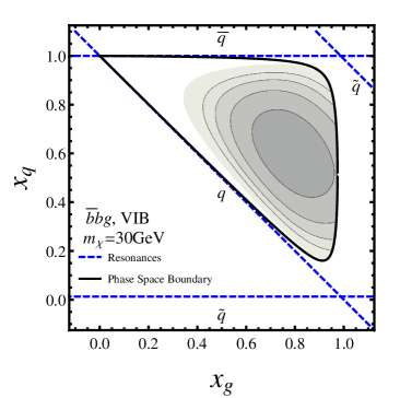
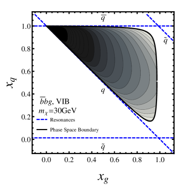
Figure 17: Double differential annihilation rate within phase space boundary for neutralino annihilation into $\bar{b}bg$ for the full rate $d^{2}N_{B}^{\mathrm{full}}/dx_{g}dx_{q}$ (left) and the FSR subtracted rate $d^{2}\tilde{N}_{\bar{q}qg}/dx_{g}dx_{q}$ (right), as defined in Eq. (32). In both figures $m_{\chi}=30$ GeV and we assume a maximal VIB scenario ($g^{L}_{\tilde{q}q\chi}=g^{R}_{\tilde{q}q\chi}=1$, $m_{\tilde{q}}=m_{\chi}$), the neutralino mass being chosen relatively low such as to demonstrate the effect of the quark mass on the shape of the phase-space boundary (solid line). The logarithmic color scale spans the range $-0.2\leq\log_{10}\left(\frac{d^{2}N_{B}^{\textrm{full}}}{dx_{g}dx_{q}}\right)\leq 0.9$, white inside the solid line exceeds the upper bound in the range, and black exceeds the lower. Plotted alongside amplitudes are the quark and squark resonances present in the diagrams.

$$\frac{d^{2}\tilde{N}_{\bar{q}qg}^{m_{\tilde{q}}\to\infty,\mathrm{mix}}}{dx_{q}dx_{g}}\propto 1+\frac{\sqrt{\mu}x_{g}^{3}-\mu x_{g}^{2}}{4(1-x_{q})(x_{g}+x_{q}-1)}\,,$$ (37)

and for vanishing squark mixings ($g^{L}_{\tilde{q}_{L}q\chi}=g^{R}_{\tilde{q}_{R}q\chi}=0$),

$$\frac{d^{2}\tilde{N}_{\bar{q}qg}^{m_{\tilde{q}}\rightarrow\infty,\cancel{\mathrm{mix}}}}{dx_{q}dx_{g}}\propto\frac{x_{g}^{3}}{(1-x_{q})(x_{g}+x_{q}-1)}\,.$$ (38)

Importantly the subtracted 3-body spectrum as defined in Eq. (32) is always divergence free, with the IR and co-linear divergences in the double differential rate $d^{2}N_{B}^{\textrm{full}}/dx_{g}dx_{q}$ canceled by the same divergence occurring in the simplified model. This is expected from the general discussion in Appendix A, but it is instructive to show this explicitly for the specific case of a maximal VIB spectrum as defined above. For this sake, we plot in Fig. 17 both the subtracted rate ${d^{2}\tilde{N}_{\bar{q}qg}}/{dx_{g}dx_{q}}$ and its un-subtracted analogue $d^{2}N_{B}^{\textrm{full}}/dx_{g}dx_{q}$, i.e. only the first term in Eq. (32); in both cases we choose a $\bar{b}bg$ final state and a neutralino mass of 30 GeV. We also indicate in the figure the location of the divergences that result from the quark or squark propagators being on shell (blue dashed lines).

The un-subtracted rate clearly diverges on approaching the on-shell conditions for the quark ($x_{q}+x_{g}=1$) and antiquark ($x_{q}=1$) propagators. This is the well-known co- linear divergence, regulated by the small but non-zero quark mass that limits the available phase-space to $x_{q}<1-\frac{\mu x_{g}}{4(1-x_{g})}+\mathcal{O}(\mu^{2})$ and $x_{q}+x_{g}>1+\frac{\mu x_{g}}{4(1-x_{g})}+\mathcal{O}(\mu^{2})$. Also the standard infrared divergence for $x_{g}\to 0$ is clearly visible (which can be regulated in a very similar way by introducing a fictitious gluon mass). On the other hand the subtracted rate $d\tilde{N}_{\bar{q}qg}/dx_{g}$ is finite over the whole region spanned by $\{x_{q}\leq 1\}\cap\{x_{q}+x_{g}\geq 1\}\cap\{x_{g}\leq 1\}$, dying completely off for infrared photons ($x_{g}\ll 1$). As a result, $d\tilde{N}_{\bar{q}qg}/dx_{g}$ now clearly peaks for large values of $x_{g}$, in particular when most of the remaining energy is carried by either $q$ or $\bar{q}$. Note that this is different to the effect of the co-linear divergences – which have been subtracted – and rather due to the presence of squark propagator resonances at $x_{q}=(3-2x_{g}-\mu_{q}+\mu_{\tilde{q}})/2$ and $x_{q}=(1+\mu_{q}-\mu_{\tilde{q}})/2$, respectively. Obviously, this observation reinforces the naive interpretation of VIB being due to gluon emission from virtual squarks.

Phenomenologically, an on average larger gluon energy leads to a higher antiproton multiplicity. This can be explained by the fact that, due to its self-coupling, a high-energy gluon fragments more easily into high-energy partons than a high-energy quark. Indeed, we find that the antiproton spectrum that results from a pure VIB double-differential rate lies about half-way between that from $\bar{q}q$ and $gg$ final states. For $\mu_{\tilde{q}}\rightarrow\infty$, on the other hand, the squarks will decouple and the double-differential rate will no longer be strongly peaked towards $x_{g}\to 1$. As a result the spectrum will flatten and become more ‘3-body like’, with the available energy being equally shared between all final states. We should thus naively expect that $\mu_{\tilde{q}}\rightarrow 1$ and $\mu_{\tilde{q}}\rightarrow\infty$ constitute the two limiting cases for the shape of both $d\tilde{N}_{\bar{q}qg}/dT$ and the resulting antiproton spectrum. These are the two limits used to fit the true model dependent spectrum, as discussed in the main text.

References

- Wess and Zumino (1974) J. Wess and B. Zumino, Nucl.Phys. B70, 39 (1974).
- Bechtle et al. (2014) P. Bechtle, K. Desch, H. K. Dreiner, M. Hamer, M. Krämer, et al., (2014), arXiv:1410.6035 [hep-ph] .
- Buchmueller et al. (2014) O. Buchmueller, R. Cavanaugh, A. De Roeck, M. Dolan, J. Ellis, et al., Eur.Phys.J. C74, 2922 (2014), arXiv:1312.5250 [hep-ph] .
- Strege et al. (2014) C. Strege, G. Bertone, G. J. Besjes, S. Caron, R. Ruiz de Austri, A. Strubig, and R. Trotta, JHEP 09, 081 (2014), arXiv:1405.0622 [hep-ph] .
- Cahill-Rowley et al. (2015) M. Cahill-Rowley, R. Cotta, A. Drlica-Wagner, S. Funk, J. Hewett, A. Ismail, T. Rizzo, and M. Wood, Phys. Rev. D91, 055011 (2015), arXiv:1405.6716 [hep-ph] .
- Roszkowski et al. (2015) L. Roszkowski, E. M. Sessolo, and A. J. Williams, JHEP 02, 014 (2015), arXiv:1411.5214 [hep-ph] .
- de Vries et al. (2015) K. J. de Vries et al., Eur. Phys. J. C75, 422 (2015), arXiv:1504.03260 [hep-ph] .
- Aad et al. (2015a) G. Aad et al. (ATLAS), JHEP 10, 134 (2015a), arXiv:1508.06608 [hep-ex] .
- Ade et al. (2015) P. Ade et al. (Planck), (2015), arXiv:1502.01589 [astro-ph.CO] .
- Jungman et al. (1996) G. Jungman, M. Kamionkowski, and K. Griest, Phys.Rept. 267, 195 (1996), arXiv:hep-ph/9506380 [hep-ph] .
- Bertone et al. (2005) G. Bertone, D. Hooper, and J. Silk, Phys.Rept. 405, 279 (2005), arXiv:hep-ph/0404175 [hep-ph] .
- Akerib et al. (2014) D. Akerib et al. (LUX), Phys.Rev.Lett. 112, 091303 (2014), arXiv:1310.8214 [astro-ph.CO] .
- Ackermann et al. (2015) M. Ackermann et al. (Fermi-LAT), Phys. Rev. Lett. 115, 231301 (2015), arXiv:1503.02641 [astro-ph.HE] .
- Bergström et al. (2013) L. Bergström, T. Bringmann, I. Cholis, D. Hooper, and C. Weniger, Phys.Rev.Lett. 111, 171101 (2013), arXiv:1306.3983 [astro-ph.HE] .
- Edsjö and Gondolo (1997) J. Edsjö and P. Gondolo, Phys.Rev. D56, 1879 (1997), arXiv:hep-ph/9704361 [hep-ph] .
- Ellis et al. (2000) J. R. Ellis, T. Falk, K. A. Olive, and M. Srednicki, Astropart.Phys. 13, 181 (2000), arXiv:hep-ph/9905481 [hep-ph] .
- Kawagoe and Nojiri (2006) K. Kawagoe and M. M. Nojiri, Phys. Rev. D74, 115011 (2006), arXiv:hep-ph/0606104 [hep-ph] .
- Arbey et al. (2015) A. Arbey, M. Battaglia, and F. Mahmoudi, (2015), arXiv:1506.02148 [hep-ph] .
- Boehm et al. (2000a) C. Boehm, A. Djouadi, and Y. Mambrini, Phys. Rev. D61, 095006 (2000a), arXiv:hep-ph/9907428 [hep-ph] .
- Agrawal and Frugiuele (2014) P. Agrawal and C. Frugiuele, JHEP 1401, 115 (2014), arXiv:1304.3068 [hep-ph] .
- Blanke et al. (2013) M. Blanke, G. F. Giudice, P. Paradisi, G. Perez, and J. Zupan, JHEP 1306, 022 (2013), arXiv:1302.7232 [hep-ph] .
- Hisano et al. (2011) J. Hisano, K. Ishiwata, and N. Nagata, Phys.Lett. B706, 208 (2011), arXiv:1110.3719 [hep-ph] .
- Garny et al. (2012a) M. Garny, A. Ibarra, M. Pato, and S. Vogl, JCAP 1211, 017 (2012a), arXiv:1207.1431 [hep-ph] .
- Asano et al. (2012) M. Asano, T. Bringmann, and C. Weniger, Phys.Lett. B709, 128 (2012), arXiv:1112.5158 [hep-ph] .
- Weiler (2012) T. J. Weiler, AIP Conf.Proc. 1534, 165 (2012), arXiv:1301.0021 [hep-ph] .
- Bergström (1989) L. Bergström, Phys.Lett. B225, 372 (1989).
- Flores et al. (1989) R. Flores, K. A. Olive, and S. Rudaz, Phys.Lett. B232, 377 (1989).
- Bringmann et al. (2008) T. Bringmann, L. Bergström, and J. Edsjö, JHEP 0801, 049 (2008), arXiv:0710.3169 [hep-ph] .
- Bergström et al. (2008) L. Bergström, T. Bringmann, and J. Edsjö, Phys.Rev. D78, 103520 (2008), arXiv:0808.3725 [astro-ph] .
- Baltz and Bergström (2003) E. Baltz and L. Bergström, Phys.Rev. D67, 043516 (2003), arXiv:hep-ph/0211325 [hep-ph] .
- Beacom et al. (2005) J. F. Beacom, N. F. Bell, and G. Bertone, Phys. Rev. Lett. 94, 171301 (2005), arXiv:astro-ph/0409403 [astro-ph] .
- Bell and Jacques (2009) N. F. Bell and T. D. Jacques, Phys. Rev. D79, 043507 (2009), arXiv:0811.0821 [astro-ph] .
- Barger et al. (2009) V. Barger, Y. Gao, W. Y. Keung, and D. Marfatia, Phys. Rev. D80, 063537 (2009), arXiv:0906.3009 [hep-ph] .
- Bringmann et al. (2012) T. Bringmann, X. Huang, A. Ibarra, S. Vogl, and C. Weniger, JCAP 1207, 054 (2012), arXiv:1203.1312 [hep-ph] .
- Bergström (2012) L. Bergström, Phys.Rev. D86, 103514 (2012), arXiv:1208.6082 [hep-ph] .
- Garny et al. (2013) M. Garny, A. Ibarra, M. Pato, and S. Vogl, JCAP 1312, 046 (2013), arXiv:1306.6342 [hep-ph] .
- Toma (2013) T. Toma, Phys.Rev.Lett. 111, 091301 (2013), arXiv:1307.6181 [hep-ph] .
- Giacchino et al. (2013) F. Giacchino, L. Lopez-Honorez, and M. H. Tytgat, JCAP 1310, 025 (2013), arXiv:1307.6480 [hep-ph] .
- Kachelriess et al. (2009) M. Kachelriess, P. D. Serpico, and M. A. Solberg, Phys. Rev. D80, 123533 (2009), arXiv:0911.0001 [hep-ph] .
- Bell et al. (2011a) N. F. Bell, J. B. Dent, T. D. Jacques, and T. J. Weiler, Phys.Rev. D83, 013001 (2011a), arXiv:1009.2584 [hep-ph] .
- Yaguna (2010) C. E. Yaguna, Phys. Rev. D81, 075024 (2010), arXiv:1003.2730 [hep-ph] .
- Bell et al. (2011b) N. F. Bell, J. B. Dent, T. D. Jacques, and T. J. Weiler, Phys.Rev. D84, 103517 (2011b), arXiv:1101.3357 [hep-ph] .
- Ciafaloni et al. (2011a) P. Ciafaloni, M. Cirelli, D. Comelli, A. De Simone, A. Riotto, et al., JCAP 1106, 018 (2011a), arXiv:1104.2996 [hep-ph] .
- Bell et al. (2011c) N. F. Bell, J. B. Dent, A. J. Galea, T. D. Jacques, L. M. Krauss, et al., Phys.Lett. B706, 6 (2011c), arXiv:1104.3823 [hep-ph] .
- Garny et al. (2011) M. Garny, A. Ibarra, and S. Vogl, JCAP 1107, 028 (2011), arXiv:1105.5367 [hep-ph] .
- Ciafaloni et al. (2011b) P. Ciafaloni, M. Cirelli, D. Comelli, A. De Simone, A. Riotto, et al., JCAP 1110, 034 (2011b), arXiv:1107.4453 [hep-ph] .
- Ciafaloni et al. (2012) P. Ciafaloni, D. Comelli, A. De Simone, A. Riotto, and A. Urbano, JCAP 1206, 016 (2012), arXiv:1202.0692 [hep-ph] .
- Fukushima et al. (2012) K. Fukushima, Y. Gao, J. Kumar, and D. Marfatia, Phys.Rev. D86, 076014 (2012), arXiv:1208.1010 [hep-ph] .
- Bell et al. (2012) N. F. Bell, A. J. Brennan, and T. D. Jacques, JCAP 1210, 045 (2012), arXiv:1206.2977 [hep-ph] .
- Bringmann and Calore (2014) T. Bringmann and F. Calore, Phys.Rev.Lett. 112, 071301 (2014), arXiv:1308.1089 [hep-ph] .
- Drees et al. (1994) M. Drees, G. Jungman, M. Kamionkowski, and M. M. Nojiri, Phys.Rev. D49, 636 (1994), arXiv:hep-ph/9306325 [hep-ph] .
- Garny et al. (2012b) M. Garny, A. Ibarra, and S. Vogl, JCAP 1204, 033 (2012b), arXiv:1112.5155 [hep-ph] .
- Gondolo et al. (2004) P. Gondolo, J. Edsjo, P. Ullio, L. Bergstrom, M. Schelke, and E. A. Baltz, JCAP 0407, 008 (2004), arXiv:astro-ph/0406204 [astro-ph] .
- (54) P. Gondolo, E. Edsjö, P. Ullio, L. Bergström, M. Schelke, E. A. Baltz, T. Bringmann, and G. Duda, http://www.darksusy.org.
- Herrmann and Klasen (2007) B. Herrmann and M. Klasen, Phys.Rev. D76, 117704 (2007), arXiv:0709.0043 [hep-ph] .
- Herrmann et al. (2009a) B. Herrmann, M. Klasen, and K. Kovar̆ik, Phys.Rev. D80, 085025 (2009a), arXiv:0907.0030 [hep-ph] .
- Herrmann et al. (2009b) B. Herrmann, M. Klasen, and K. Kovarik, Phys.Rev. D79, 061701 (2009b), arXiv:0901.0481 [hep-ph] .
- Herrmann et al. (2014) B. Herrmann, M. Klasen, K. Kovarik, M. Meinecke, and P. Steppeler, Phys. Rev. D89, 114012 (2014), arXiv:1404.2931 [hep-ph] .
- Bringmann and Weniger (2012) T. Bringmann and C. Weniger, Phys.Dark Univ. 1, 194 (2012), arXiv:1208.5481 [hep-ph] .
- Sjöstrand et al. (2008) T. Sjöstrand, S. Mrenna, and P. Z. Skands, Comput.Phys.Commun. 178, 852 (2008), arXiv:0710.3820 [hep-ph] .
- Sjostrand et al. (2006) T. Sjostrand, S. Mrenna, and P. Z. Skands, JHEP 0605, 026 (2006), arXiv:hep-ph/0603175 [hep-ph] .
- Ginzburg and Syrovatskii (1964) V. L. Ginzburg and S. I. Syrovatskii, The Origin of Cosmic Rays, New York: Macmillan (1964).
- Bringmann et al. (2014) T. Bringmann, M. Vollmann, and C. Weniger, Phys.Rev. D90, 123001 (2014), arXiv:1406.6027 [astro-ph.HE] .
- Gleeson and Axford (1968) L. Gleeson and W. Axford, Astrophys.J. 154, 1011 (1968).
- Perko (1987) J. S. Perko, Astron. Astrophys. 184, 119 (1987).
- Bringmann and Salati (2007) T. Bringmann and P. Salati, Phys.Rev. D75, 083006 (2007), arXiv:astro-ph/0612514 [astro-ph] .
- Donato et al. (2001) F. Donato, D. Maurin, P. Salati, A. Barrau, G. Boudoul, et al., Astrophys.J. 563, 172 (2001), arXiv:astro-ph/0103150 [astro-ph] .
- Evoli et al. (2012) C. Evoli, I. Cholis, D. Grasso, L. Maccione, and P. Ullio, Phys.Rev. D85, 123511 (2012), arXiv:1108.0664 [astro-ph.HE] .
- Rolke et al. (2005) W. A. Rolke, A. M. Lopez, and J. Conrad, Nucl.Instrum.Meth. A551, 493 (2005), arXiv:physics/0403059 [physics] .
- Adriani et al. (2013) O. Adriani et al., JETP Lett. 96, 621 (2013), [Pisma Zh. Eksp. Teor. Fiz.96,693(2012)].
- Talk at the ‘AMS Days at CERN’ (2015) Talk at the ‘AMS Days at CERN’, AMS-02 Collaboration (2015), http://indico.cern.ch/event/381134/.
- Bergstrom and Snellman (1988) L. Bergstrom and H. Snellman, Phys. Rev. D37, 3737 (1988).
- Donato et al. (2004) F. Donato, N. Fornengo, D. Maurin, and P. Salati, Phys. Rev. D69, 063501 (2004), arXiv:astro-ph/0306207 [astro-ph] .
- Achard et al. (2004) P. Achard et al. (L3), Phys. Lett. B580, 37 (2004), arXiv:hep-ex/0310007 [hep-ex] .
- Group (2004) L. S. W. Group, ALEPH, DELPHI, L3, OPAL Experiments, LEPSUSYWG/04-02.1 (2004), http://lepsusy.web.cern.ch/lepsusy/www/ squarks_summer04/stop_combi_208_final.html.
- Aad et al. (2014) G. Aad et al. (ATLAS), JHEP 09, 176 (2014), arXiv:1405.7875 [hep-ex] .
- Aad et al. (2015b) G. Aad et al. (ATLAS), Eur. Phys. J. C75, 510 (2015b), arXiv:1506.08616 [hep-ex] .
- Aad et al. (2015c) G. Aad et al. (ATLAS), JHEP 10, 054 (2015c), arXiv:1507.05525 [hep-ex] .
- Chatrchyan et al. (2014) S. Chatrchyan et al. (CMS), JHEP 06, 055 (2014), arXiv:1402.4770 [hep-ex] .
- Olive et al. (2014) K. A. Olive et al. (Particle Data Group), Chin. Phys. C38, 090001 (2014).
- Atwood et al. (2009) W. B. Atwood et al. (Fermi-LAT), Astrophys. J. 697, 1071 (2009), arXiv:0902.1089 [astro-ph.IM] .
- Gondolo and Gelmini (1991) P. Gondolo and G. Gelmini, Nucl.Phys. B360, 145 (1991).
- Hisano et al. (2007) J. Hisano, S. Matsumoto, M. Nagai, O. Saito, and M. Senami, Phys.Lett. B646, 34 (2007), arXiv:hep-ph/0610249 [hep-ph] .
- Hryczuk et al. (2011) A. Hryczuk, R. Iengo, and P. Ullio, JHEP 1103, 069 (2011), arXiv:1010.2172 [hep-ph] .
- Hryczuk (2011) A. Hryczuk, Phys.Lett. B699, 271 (2011), arXiv:1102.4295 [hep-ph] .
- Freitas (2007) A. Freitas, Phys.Lett. B652, 280 (2007), arXiv:0705.4027 [hep-ph] .
- Kovarik and Herrmann (2010) K. Kovarik and B. Herrmann, AIP Conf.Proc. 1200, 1075 (2010), arXiv:0910.0941 [hep-ph] .
- Boudjema et al. (2011) F. Boudjema, G. Drieu La Rochelle, and S. Kulkarni, Phys.Rev. D84, 116001 (2011), arXiv:1108.4291 [hep-ph] .
- Chatterjee et al. (2012) A. Chatterjee, M. Drees, and S. Kulkarni, Phys.Rev. D86, 105025 (2012), arXiv:1209.2328 [hep-ph] .
- Martin (2010) S. P. Martin, Adv.Ser.Direct.High Energy Phys. 21, 1 (2010), arXiv:hep-ph/9709356 [hep-ph] .
- Le Boulc’ H (2013) Q. Le Boulc’ H, Coannihilation neutralino-stop dans le MSSM : violation de saveur, corrections radiatives et leur impact sur la densité relique de matière noire., Ph.D. thesis, Université de Grenoble (2013).
- Boehm et al. (2000b) C. Boehm, A. Djouadi, and M. Drees, Phys. Rev. D62, 035012 (2000b), arXiv:hep-ph/9911496 [hep-ph] .
- Ellis et al. (2003) J. R. Ellis, K. A. Olive, and Y. Santoso, Astropart.Phys. 18, 395 (2003), arXiv:hep-ph/0112113 [hep-ph] .
- Bednyakov et al. (2002) V. Bednyakov, H. Klapdor-Kleingrothaus, and V. Gronewold, Phys.Rev. D66, 115005 (2002), arXiv:hep-ph/0208178 [hep-ph] .
- Santoso (2003) Y. Santoso, Nucl.Phys.Proc.Suppl. 124, 166 (2003), arXiv:hep-ph/0205026 [hep-ph] .
- Baer et al. (2002) H. Baer, C. Balazs, and A. Belyaev, JHEP 0203, 042 (2002), arXiv:hep-ph/0202076 [hep-ph] .
- Edsjo et al. (2003) J. Edsjo, M. Schelke, P. Ullio, and P. Gondolo, JCAP 0304, 001 (2003), arXiv:hep-ph/0301106 [hep-ph] .
- Ajaib et al. (2012) M. A. Ajaib, T. Li, and Q. Shafi, Phys. Rev. D85, 055021 (2012), arXiv:1111.4467 [hep-ph] .
- Diaz-Cruz et al. (2007) J. L. Diaz-Cruz, J. R. Ellis, K. A. Olive, and Y. Santoso, JHEP 05, 003 (2007), arXiv:hep-ph/0701229 [HEP-PH] .
- Huitu et al. (2011) K. Huitu, L. Leinonen, and J. Laamanen, Phys.Rev. D84, 075021 (2011), arXiv:1107.2128 [hep-ph] .
- Ellis et al. (2014) J. Ellis, K. A. Olive, and J. Zheng, Eur.Phys.J. C74, 2947 (2014), arXiv:1404.5571 [hep-ph] .
- Ibarra et al. (2015) A. Ibarra, A. Pierce, N. Shah, and S. Vogl, Phys.Rev. D91, 095018 (2015), arXiv:1501.03164 [hep-ph] .
- Aad et al. (2012) G. Aad et al. (ATLAS), Phys. Lett. B716, 1 (2012), arXiv:1207.7214 [hep-ex] .
- Chatrchyan et al. (2012) S. Chatrchyan et al. (CMS), Phys. Lett. B716, 30 (2012), arXiv:1207.7235 [hep-ex] .
- Balazs et al. (2004) C. Balazs, M. Carena, and C. E. M. Wagner, Phys. Rev. D70, 015007 (2004), arXiv:hep-ph/0403224 [hep-ph] .
- Harz et al. (2013a) J. Harz, B. Herrmann, M. Klasen, K. Kovarik, and Q. L. Boulc’h, Phys.Rev. D87, 054031 (2013a), arXiv:1212.5241 .
- Harz (2013) J. Harz, Supersymmetric QCD Corrections and Phenomenological Studies in Relation to Coannihilation of Dark Matter, Ph.D. thesis, University of Hamburg (2013).
- Harz et al. (2013b) J. Harz, B. Herrmann, M. Klasen, K. Kovarik, and Q. Le Boulc’h, PoS Corfu2012, 075 (2013b), arXiv:1302.3525 [hep-ph] .
- Harz et al. (2015a) J. Harz, B. Herrmann, M. Klasen, K. Kovařík, and M. Meinecke, Phys.Rev. D91, 034012 (2015a), arXiv:1410.8063 [hep-ph] .
- Harz et al. (2015b) J. Harz, B. Herrmann, M. Klasen, and K. Kovarik, Phys.Rev. D91, 034028 (2015b), arXiv:1409.2898 [hep-ph] .
- Belanger et al. (2014) G. Belanger, F. Boudjema, A. Pukhov, and A. Semenov, Comput. Phys. Commun. 185, 960 (2014), arXiv:1305.0237 [hep-ph] .
- Bringmann et al. (2015) T. Bringmann, F. Calore, A. Galea, and M. Garny, in prep. (2015).
- (113) http://dmnlo.hepforge.org.
- James and Roos (1975) F. James and M. Roos, Comput.Phys.Commun. 10, 343 (1975).
- Calore (2013) F. Calore, Unveiling Dark Matter through Gamma Rays: Spectral Features, Spatial Signatures and Astrophysical Backgrounds, Ph.D. thesis, University of Hamburg (2013).
- Bergström et al. (2005) L. Bergström, T. Bringmann, M. Eriksson, and M. Gustafsson, Phys.Rev.Lett. 94, 131301 (2005), arXiv:astro-ph/0410359 [astro-ph] .
- Birkedal et al. (2005) A. Birkedal, K. T. Matchev, M. Perelstein, and A. Spray, (2005), arXiv:hep-ph/0507194 [hep-ph] .
- Kinoshita (1962) T. Kinoshita, J.Math.Phys. 3, 650 (1962).
- Bloch and Nordsieck (1937) F. Bloch and A. Nordsieck, Phys.Rev. 52, 54 (1937).
- Braaten and Leveille (1980) E. Braaten and J. Leveille, Phys.Rev. D22, 715 (1980).
- Drees and Hikasa (1990a) M. Drees and K. Hikasa, Phys.Lett. B240, 455 (1990a).
- Larin (1993) S. Larin, Phys.Lett. B303, 113 (1993), arXiv:hep-ph/9302240 [hep-ph] .
- Berends et al. (1973) F. A. Berends, K. Gaemer, and R. Gastmans, Nucl.Phys. B57, 381 (1973).
- Berends et al. (1983) F. A. Berends, R. Kleiss, S. Jadach, and Z. Was, Acta Phys.Polon. B14, 413 (1983).
- Akhundov et al. (1985) A. Akhundov, D. Y. Bardin, O. Fedorenko, and T. Riemann, Sov.J.Nucl.Phys. 42, 762 (1985).
- Peskin and Schroeder (1995) M. E. Peskin and D. V. Schroeder, (1995).
- Drees and Hikasa (1990b) M. Drees and K.-i. Hikasa, Phys.Rev. D41, 1547 (1990b).
- Reinders et al. (1980) L. Reinders, H. Rubinstein, and S. Yazaki, Phys.Lett. B94, 203 (1980).
- Chetyrkin and Kühn (1990) K. Chetyrkin and J. H. Kühn, Phys.Lett. B248, 359 (1990).
- Chetyrkin et al. (2000) K. Chetyrkin, J. H. Kuhn, and M. Steinhauser, Comput.Phys.Commun. 133, 43 (2000), arXiv:hep-ph/0004189 [hep-ph] .
- Carena et al. (2000) M. Carena, D. Garcia, U. Nierste, and C. E. Wagner, Nucl.Phys. B577, 88 (2000), arXiv:hep-ph/9912516 [hep-ph] .
- Guasch et al. (2003) J. Guasch, P. Häfliger, and M. Spira, Phys.Rev. D68, 115001 (2003), arXiv:hep-ph/0305101 [hep-ph] .
- Herrmann (2015) B. Herrmann, personal communication (2015).