The Bouncy Particle Sampler: A Non-Reversible Rejection-Free Markov Chain Monte Carlo Method

Abstract

Many Markov chain Monte Carlo techniques currently available rely on discrete-time reversible Markov processes whose transition kernels are variations of the Metropolis–Hastings algorithm. We explore and generalize an alternative scheme recently introduced in the physics literature [27] where the target distribution is explored using a continuous-time non-reversible piecewise-deterministic Markov process. In the Metropolis–Hastings algorithm, a trial move to a region of lower target density, equivalently of higher “energy”, than the current state can be rejected with positive probability. In this alternative approach, a particle moves along straight lines around the space and, when facing a high energy barrier, it is not rejected but its path is modified by bouncing against this barrier. By reformulating this algorithm using inhomogeneous Poisson processes, we exploit standard sampling techniques to simulate exactly this Markov process in a wide range of scenarios of interest. Additionally, when the target distribution is given by a product of factors dependent only on subsets of the state variables, such as the posterior distribution associated with a probabilistic graphical model, this method can be modified to take advantage of this structure by allowing computationally cheaper “local” bounces which only involve the state variables associated to a factor, while the other state variables keep on evolving. In this context, by leveraging techniques from chemical kinetics, we propose several computationally efficient implementations. Experimentally, this new class of Markov chain Monte Carlo schemes compares favorably to state-of-the-art methods on various Bayesian inference tasks, including for high dimensional models and large data sets.

^∗Department of Statistics, University of British Columbia, Canada.

^†Mathematics Institute and Department of Statistics, University of Warwick, UK.

^‡Department of Statistics, University of Oxford, UK.

Keywords: Inhomogeneous Poisson process; Markov chain Monte Carlo; Piecewise deterministic Markov process; Probabilistic graphical models; Rejection-free simulation.

1 Introduction

Markov chain Monte Carlo (MCMC) methods are standard tools to sample from complex high-dimensional probability measures. Many MCMC schemes available at present are based on the Metropolis-Hastings (MH) algorithm and their efficiency is strongly dependent on the ability of the user to design proposal distributions capturing the main features of the target distribution; see [20] for a comprehensive review. We examine, analyze and generalize here a different approach to sample from distributions on $\mathbb{R}^{d}$ that has been recently proposed in the physics literature [27]. Let the energy be defined as minus the logarithm of an unnormalized version of the target density. In this methodology, a particle explores the space by moving along straight lines and, when it faces a high energy barrier, it bounces against the contour lines of this energy. This non-reversible rejection-free MCMC method will be henceforth referred to as the Bouncy Particle Sampler (BPS). This algorithm and closely related schemes have already been adopted to simulate complex physical systems such as hard spheres, polymers and spin models [19, 22, 23, 25]. For these models, it has been demonstrated experimentally that such methods can outperform state-of-the-art MCMC methods by up to several orders of magnitude.

However, the implementation of the BPS proposed in [27] is not applicable to most target distributions arising in statistics. In this article we make the following contributions:

Simulation schemes based on inhomogeneous Poisson processes:

by reformulating explicitly the bounces times of the BPS as the first arrival times of inhomogeneous Poisson Processes (PP), we leverage standard sampling techniques [8, Chapter 6] and methods from chemical kinetics [31] to obtain new computationally efficient ways to simulate the BPS process for a large class of target distributions.

Factor graphs:

when the target distribution can be expressed as a factor graph [32], a representation generalizing graphical models where the target is given by a product of factors and each factor can be a function of only a subset of variables, we adapt a physical multi-particle system method discussed in [27, Section III] to achieve additional computational efficiency. This local version of the BPS only manipulates a restricted subset of the state components at each bounce but results in a change of all state components, not just the one being updated contrary the Gibbs sampler.

Ergodicity analysis:

we present a proof of the ergodicity of BPS when the velocity of the particle is additionally refreshed at the arrival times of an homogeneous PP. When this refreshment step is not carried out, we exhibit a counter-example where ergodicity does not hold.

Efficient refreshment:

we propose alternative refreshment schemes and compare their computational efficiency experimentally.

Empirically, these new MCMC schemes compare favorably to state-of-the-art MCMC methods on various Bayesian inference problems, including for high-dimensional scenarios and large data sets. Several additional original extensions of the BPS including versions of the algorithm which are applicable to mixed continuous-discrete distributions, distributions restricted to a compact support and a method relying on the use of curved dynamics instead of straight lines can be found in [5]. For brevity, these are not discussed here.

The rest of this article is organized as follows. In Section 2, we introduce the basic version of the BPS, propose original ways to implement it and prove its ergodicity under weak assumptions. Section 3 presents a modification of the basic BPS which exploits a factor graph representation of the target distribution and develops computationally efficient implementations of this scheme. In Section 4, we demonstrate this methodology on various Bayesian models. The proofs are given in the Appendix and the Supplementary Material.

2 The bouncy particle sampler

2.1 Problem statement and notation

Consider a probability distribution $\pi$ on $\mathbb{R}^{d},$ equipped with the Borel $\sigma$-algebra $\mathcal{B}(\mathbb{R}^{d})$. We assume that $\pi$ admits a probability density with respect to the Lebesgue measure ${\rm d}x$ and slightly abuse notation by denoting also this density by $\pi$. In most practical scenarios, we only have access to an unnormalized version of this density, that is

$$\pi\left(x\right)=\frac{\gamma\left(x\right)}{\mathcal{Z}},$$

where $\gamma:\mathbb{R}^{d}\rightarrow(0,\infty)$ can be evaluated pointwise but the normalizing constant $\mathcal{Z}=\int_{\mathbb{R}^{d}}\gamma\left(x\right){\rm d}x$ is unknown. We call

$$U\left(x\right)=-\mathrm{log}\leavevmode\nobreak\ \gamma\left(x\right)$$

the associated energy, which is assumed continuously differentiable, and we denote by $\nabla U\left(x\right)=\left(\frac{\partial U\left(x\right)}{\partial x_{1}},\ldots,\frac{\partial U\left(x\right)}{\partial x_{d}}\right)^{\top}$ the gradient of $U$ evaluated at $x$. We are interested in approximating numerically the expectation of arbitrary test functions $\varphi:\mathbb{R}^{d}\rightarrow\mathbb{R}$ with respect to $\pi$.

2.2 Algorithm description

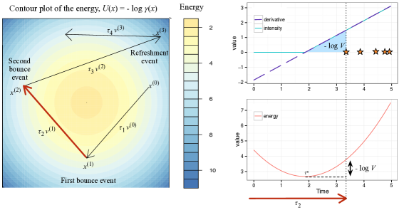
Figure 1: Illustration of BPS on a standard bivariate Gaussian distribution. Left and top right: see Section 2.2; bottom right: see Example 1.

The BPS methodology introduced in [27] simulates a continuous piecewise linear trajectory $\left\{x\left(t\right)\right\}_{t\geq 0}$ in $\mathbb{R}^{d}$. It has been informally derived as a continuous-time limit of the Metropolis algorithm in [27]. Each segment in the trajectory is specified by an initial position $x^{\left(i\right)}\in\mathbb{R}^{d}$, a length $\tau_{i+1}\in\mathbb{R}^{+}$ and a velocity $v^{\left(i\right)}\in\mathbb{R}^{d}$ (example shown in Figure 1, left). We denote the times where the velocity changes by $t_{i}=\sum_{j=1}^{i}\tau_{j}$ for $i\geq 1$, and set $t_{0}=0$ for convenience. The position at time $t\in[t_{i},t_{i+1})$ is thus interpolated linearly, $x\left(t\right)=x^{\left(i\right)}+v^{\left(i\right)}\left(t-t_{i}\right)$, and each segment is connected to the next, $x^{\left(i+1\right)}=x^{\left(i\right)}+v^{\left(i\right)}\tau_{i+1}$. The length of these segments is governed by an inhomogeneous PP of intensity function $\lambda:\mathbb{R}^{d}\times\mathbb{R}^{d}\rightarrow[0,\infty)$

$$\lambda\left(x,v\right)=\mathrm{max}\left\{0,\left\langle\nabla U\left(x\right),v\right\rangle\right\}.$$ (1)

When the particle bounces, its velocity is updated in the same way as a Newtonian elastic collision on the hyperplane tangential to the gradient of the energy. Formally, the velocity after bouncing is given by

$$R\left(x\right)v=\left(I_{d}-2\frac{\nabla U\left(x\right)\left\{\nabla U\left(x\right)\right\}^{\top}}{\left\|\nabla U\left(x\right)\right\|^{2}}\right)v=v-2\frac{\left\langle\nabla U\left(x\right),v\right\rangle}{\left\|\nabla U\left(x\right)\right\|^{2}}\nabla U\left(x\right),$$ (2)

where $I_{d}$ denotes the $d\times d$ identity matrix, $\|\cdot\|$ the Euclidean norm, and $\left\langle w,z\right\rangle=w^{t}z$ the scalar product between column vectors $w,z$. [27] also refresh the velocity at periodic times. We slightly modify their approach by performing a velocity refreshment at the arrival times of a homogeneous PP of intensity $\lambda^{\mathrm{ref}}\geq 0$, $\lambda^{\mathrm{ref}}$ being a parameter of the algorithm. A similar refreshment scheme was used for a related process in [22]. Throughout the paper, we use the terminology “event” for a time at which either a bounce or a refreshment occurs. The basic version of the BPS algorithm proceeds as follows:

Algorithm 1 Basic BPS algorithm  

1. Initialize $\left(x^{\left(0\right)},v^{\left(0\right)}\right)$ arbitrarily on $\mathbb{R}^{d}\times\mathbb{R}^{d}$ and let $T$ denote the requested trajectory length.

2. For $i=1,2,\ldots$

   1. Simulate the first arrival time $\tau{}_{\mathrm{bounce}}\in(0,\infty)$ of a PP of intensity

      $$\chi\left(t\right)=\lambda(x^{\left(i-1\right)}+v^{\left(i-1\right)}t,v^{\left(i-1\right)}).$$

   2. Simulate $\tau{}_{\mathrm{ref}}\sim\mathrm{Exp\left(\lambda^{\mathrm{ref}}\right)}$.

   3. Set $\tau_{i}\leftarrow\mathrm{min}\left(\tau{}_{\mathrm{bounce}},\tau{}_{\mathrm{ref}}\right)$ and compute the next position using

      $$x^{\left(i\right)}\leftarrow x^{\left(i-1\right)}+v^{\left(i-1\right)}\tau_{i}.$$ (3)

   4. If $\tau_{i}=\tau{}_{\mathrm{ref}}$, sample the next velocity $v^{\left(i\right)}\sim\mathcal{N}\left(0_{d},I_{d}\right)$.

   5. If $\tau_{i}=\tau{}_{\mathrm{bounce}}$, compute the next velocity $v^{\left(i\right)}$ using

      $$v^{\left(i\right)}\leftarrow R\left(x^{\left(i\right)}\right)v^{\left(i-1\right)}.$$ (4)

   6. If $t_{i}=\sum_{j=1}^{i}\tau_{j}\geq T$ exit For Loop (line 2).

In the algorithm above, $\mathrm{Exp\left(\delta\right)}$ denotes the exponential distribution of rate $\delta$ and $\mathcal{N}\left(0_{d},I_{d}\right)$ the standard normal on $\mathbb{R}^{d}$. Refer to Figure 1 for an example of a trajectory generated by BPS on a standard bivariate Gaussian target distribution. An example of a bounce time simulation is shown in Figure 1, top right, for the segment between the first and second events—the intensity $\chi(t)$ (turquoise) is obtained by thresholding $\left\langle\nabla U\left(x^{(1)}+v^{\left(1\right)}t\right),v^{(1)}\right\rangle$ (purple, dashed); arrival times of the PP of intensity $\chi(t)$ are denoted by stars.

We will show further that the transition kernel of the BPS process admits $\pi$ as invariant distribution for any $\lambda^{\mathrm{ref}}\geq 0$ but it can fail to be irreducible when $\lambda^{\mathrm{ref}}=0$ as demonstrated in Section 4.1. It is thus critical to use $\lambda^{\mathrm{ref}}>0$. Our proof of invariance and ergodicity can accommodate some alternative refreshment steps 2d. One such variant, which we call restricted refreshment, samples $v^{(i)}$ uniformly on the unit hypersphere $\mathcal{S}^{d-1}=\left\{x\in\mathbb{R}^{d}:\|x\|=1\right\}$. We compare experimentally these two variants and others in Section 4.3.

2.3 Algorithms for bounce time simulation

Implementing BPS requires sampling the first arrival time $\tau$ of a one-dimensional inhomogeneous PP $\Pi$ of intensity $\chi(t)=\lambda(x+vt,v)$ given by (1). Simulating such a process is a well-studied problem; see [8, Chapter 6, Section 1.3]. We review here three methods and illustrate how they can be used to implement BPS for examples from Bayesian statistics. The first method described in Section 2.3.1 will be particularly useful when the target is log-concave, while the two others described in Section 2.3.2 and Section 2.3.3 can be applied to more general scenarios.

2.3.1 Simulation using a time-scale transformation

If we let $\varXi\left(t\right)=\int_{0}^{t}\chi\left(s\right){\rm d}s$, then the PP $\Pi$ satisfies

$${\mathbb{P}}(\tau>u) ={\mathbb{P}}(\Pi\cap[0,u)=\emptyset)=\exp(-\varXi(u)),$$

and therefore $\tau$ can be simulated from a uniform variate $V\sim\mathcal{U}\left(0,1\right)$ via the identity

$$\tau=\varXi^{-1}(-\log(V)),$$ (5)

where $\varXi^{-1}$ denotes the quantile function of $\varXi,$ $\varXi^{-1}(p)=\inf\mbox{$\left\{t:p\leq\varXi(t)\right\}$ }.$ Refer to Figure 1, top right for a graphical illustration. This identity corresponds to the method proposed in [27] to determine the bounce times and is also used in [22, 23, 25] to simulate related processes.

In general, it is not possible to obtain an analytical expression for $\tau$. However, when the target distribution is strictly log-concave and differentiable, it is possible to solve Equation (5) numerically (see Example 1 below).

Example 1.

Log-concave densities. If the energy is strictly convex (see Figure 1, bottom right), we can minimize it along the line specified by $(x,v)$

$$\tau_{*}=\mathrm{argmin}_{t:t\geq 0}\leavevmode\nobreak\ U\left(x+vt\right),$$

where $\tau_{*}$ is well defined and unique by strict convexity. On the interval $\left[0,\tau_{*}\right)$, which might be empty, we have ${\rm d}U\left(x+vt\right)/{\rm d}t<0$ and ${\rm d}U\left(x+vt\right)/{\rm d}t\geq 0$ on $\left[\tau_{*},\text{$\infty$}\right)$. The solution $\tau$ of (5) is thus necessarily such that $\tau\geq\tau_{*}$ and (5) can be rewritten using the gradient theorem as

$$\int_{\tau_{*}}^{\tau}\frac{{\rm d}U\left(x+vt\right)}{{\rm d}t}{\rm d}t=U\left(x+v\tau\right)-U\left(x+v\tau_{*}\right)=-\log V.$$ (6)

Even if we only compute $U$ pointwise through a black box, we can solve (6) through line search within machine precision.

We note that (6) also provides an informal connection between the BPS and MH algorithms. Exponentiating this equation, we get indeed

$$\frac{\pi(x+v\tau)}{\pi(x+v\tau_{*})}=V.$$

Hence, in the log-concave case, and when the particle is climbing the energy ladder (i.e., $\tau_{*}=0$), BPS can be viewed as “swapping” the order of the steps taken by the MH algorithm. In the latter, we first sample a proposal and second sample a uniform $V$ to perform an accept-reject decision. With BPS, $V$ is first drawn then the maximum distance allowed by the same MH ratio is travelled. As for the case of a particle going down the energy ladder, the behavior of BPS is simpler to understand: bouncing never occurs. We illustrate this method for Gaussian distributions.

Multivariate Gaussian distributions. Let $U\left(x\right)=\left\|x\right\|^{2}$, then simple calculations yield

$$\tau=\frac{{1}}{\left\|v\right\|^{2}}\begin{cases}-\left\langle x,v\right\rangle+\sqrt{-\left\|v\right\|^{2}\log V}&\text{if}\left\langle x,v\right\rangle\leq 0,\\ -\left\langle x,v\right\rangle+\sqrt{\left\langle x,v\right\rangle^{2}-\left\|v\right\|^{2}\log V}&\text{ otherwise.}\end{cases}$$ (7)

2.3.2 Simulation using adaptive thinning

When it is difficult to solve (5), the use of an adaptive thinning procedure provides an alternative. Assume we have access to local-in-time upper bounds $\bar{\chi}{}_{s}\left(t\right)$ on $\chi(t)$, that is

$$\bar{\chi}_{s}(t) =0\,\text{ for all }t<s,$$

$$\bar{\chi}{}_{s}(t) \geq\chi(t)\text{ for all }s\leq t\leq s+\Delta(s),$$

where $\triangle$ is a positive function (standard thinning corresponds to $\Delta=+\infty$). Assume additionally that we can simulate the first arrival time of the PP $\bar{\Pi}_{s}$ with intensity $\bar{\chi}_{s}(t)$. Such bounds can be constructed based on upper bounds on directional derivatives of $U$ provided the remainder of the Taylor expansion can be controlled. Algorithm 2 shows the pseudocode for the adaptive thinning procedure.

Algorithm 2 Simulation of the first arrival time of a PP through thinning  

1. Set $s\leftarrow 0$, $\tau\leftarrow 0$.

2. Do

   1. Set $s\leftarrow\tau$.

   2. Sample $\tau$ as the first arrival point of the PP $\bar{\Pi}_{s}$ of intensity $\bar{\chi}_{s}$.

   3. If $\bar{\Pi}_{s}=\{\emptyset\}$ then set $\tau\leftarrow s+\triangle(s)$.

   4. If $s+\triangle(s)\leq\tau$ set $s\leftarrow s+\triangle(s)$ and go to (b).

   5. While $V>\{\chi\left(\tau\right)/\bar{\chi}_{s}\left(\tau\right)\}$ where $V\sim\mathcal{U}\left(0,1\right)$.

3. Return $\tau$.

The case $V>\{\chi\left(\tau\right)/\bar{\chi}_{s}\left(\tau\right)\}$ corresponds to a rejection step in the thinning algorithm but, in contrast to rejection steps that occur in standard MCMC samplers, in the BPS algorithm this means that the particle does not bounce and just coasts. Practically, we would like ideally $\triangle$ and the ratio $\chi\left(\tau\right)/\bar{\chi}_{s}\left(\tau\right)$ to be large. Indeed this would avoid having to simulate too many candidate events from $\bar{\Pi}_{s}$ which would be rejected as these rejection steps incur a computational cost.

2.3.3 Simulation using superposition and thinning

Assume that the energy can be decomposed as

$$U\left(x\right)=\sum_{j=1}^{m}U^{[j]}\left(x\right),$$ (8)

then

$$\chi\left(t\right)\leq\sum_{j=1}^{m}\chi^{[j]}\left(t\right),$$

where $\chi^{[j]}(t)=\max\left(0,\left\langle\nabla U^{[j]}(x+tv),v\right\rangle\right)$ for $j=1,...,m$. It is therefore possible to use the thinning algorithm of Section 2.3.2 with $\bar{\chi}_{0}(t)=\sum_{j=1}^{m}\chi^{[j]}\left(t\right)$ for $t\geq 0$ (and $\Delta=+\infty$), as we can simulate from $\bar{\Pi}_{0}$ via superposition by simulating the first arrival time $\tau^{[j]}$ of each PP with intensity $\chi^{[j]}\left(t\right)\geq 0$ then returning

$$\tau=\mathrm{min}_{j=1,...,m}\leavevmode\nobreak\ \tau^{[j]}.$$

Example 2.

Exponential families. Consider a univariate exponential family with parameter $x$, observation $y,$ sufficient statistic $\phi(y)$ and log-normalizing constant $A(x)$. If we assume a Gaussian prior on $x,$ we obtain

$$U(x)=\underbrace{{x^{2}/2}}_{U^{[1]}(x)}+\underbrace{{-x\phi(y)}}_{U^{[2]}(x)}+\underbrace{{A(x)}}_{U^{[3]}(x)}.$$

The time $\tau^{[1]}$ is computed analytically in Example 1 whereas the times $\tau^{[2]}$ and $\tau^{[3]}$ are given by

$$\tau^{[2]}=\begin{cases}\frac{{\log V^{[2]}}}{v\phi(y)}&\text{if }v\phi(y)<0,\\ +\infty&\text{{otherwise,}}\end{cases}$$

and

$$\tau^{[3]} =\begin{cases}\tilde{\tau}^{[3]}&\text{if }\tilde{\tau}^{[3]}>0,\\ +\infty&\text{{otherwise,}}\end{cases}$$

with $\tilde{\tau}^{[3]}=(A^{-1}(-\log V^{[3]}+A(x))-x)/v$ and $V^{[2]},V^{[3]}\sim\mathcal{U}\left(0,1\right)$. For example, with a Poisson distribution with natural parameter $x,$ we obtain

$$\tilde{\tau}^{[3]}=\frac{\log(-\log V^{[3]}+\exp(x))-x}{v}.$$

Example 3.

Logistic regression. The class label of the data point $r\in\{1,2,\dots,R\}$ is denoted by $y_{r}\in\left\{0,1\right\}$ and its covariate $k\in\{1,2,\dots,d\}$ by $\iota_{r,k}$ where we assume that $\iota_{r,k}\geq 0$ (this assumption can be easily relaxed as demonstrated but would make the notation more complicated; see [11] for details). The parameter $x\in{\mathbb{R}}^{d}$ is assigned a standard Gaussian prior density denoted by $\psi$, yielding the posterior density

$$\pi(x)\propto\psi(x)\prod_{r=1}^{R}\frac{\exp(y{}_{r}\left\langle\iota_{r},x\right\rangle)}{1+\exp\left\langle\iota_{r},x\right\rangle}.$$ (9)

Using the superposition and thinning method (Section 2.3.3), simulation of the bounce times can be broken into subproblems corresponding to $R+1$ factors: one factor coming from the prior, with corresponding energy

$$U^{[R+1]}(x)=-\log\psi(x)=\|x\|^{2}/2+\text{constant},$$ (10)

and $R$ factors coming from the likelihood of each datapoint, with corresponding energy

$$U^{[r]}(x)=\log(1+\exp\left\langle\iota_{r},x\right\rangle)-y_{r}\left\langle\iota_{r},x\right\rangle.$$ (11)

Simulation of $\tau^{[R+1]}$ is covered in Example 1. Simulation of $\tau^{[r]}$ for $r\in\left\{1,2,\dots,R\right\}$ can be approached using thinning. In Appendix C.1, we show that

$$\chi^{[r]}(t)\leq\bar{\chi}^{[r]}=\sum_{k=1}^{d}{\mathbf{1}}[v_{k}(-1)^{y_{r}}\geq 0]\iota_{r,k}|v_{k}|.$$ (12)

Since the bound is constant for a given $v$, we sample $\tau^{[r]}$ by simulating an exponential random variable.

2.4 Estimating expectations

Given a realization of $x\left(t\right)$ over the interval $\left[0,T\right]$, where $T$ is the total trajectory length, the expectation $\int_{\mathbb{R}^{d}}\varphi\left(x\right)\pi\left({\rm d}x\right)$ of a function $\varphi:\mathbb{R}^{d}\rightarrow\mathbb{R}$ with respect to $\pi$ can be estimated using

$$\frac{1}{T}\int_{0}^{T}\varphi\left(x\left(t\right)\right){\rm d}t=\frac{1}{T}\left(\sum_{i=1}^{n-1}\int_{0}^{\tau_{i}}\varphi\left(x^{\left(i-1\right)}+v^{\left(i-1\right)}s\right){\rm d}s+\int_{0}^{t_{n}-T}\varphi\left(x^{\left(n-1\right)}+v^{\left(n-1\right)}s\right){\rm d}s\right);$$

see, e.g., [7]. When $\varphi\left(x\right)=x_{k}$, $k\in\left\{1,2,\dots,d\right\}$, we have

$$\int_{0}^{\tau_{i}}\varphi\left(x^{\left(i-1\right)}+v^{\left(i-1\right)}s\right){\rm d}s=x_{k}^{\left(i-1\right)}\tau_{i}+v_{k}^{\left(i-1\right)}\frac{\tau_{i}^{2}}{2}.$$

When the above integral is intractable, we may just discretize $x\left(t\right)$ at regular time intervals to obtain an estimator

$$\frac{1}{L}\sum_{l=0}^{L-1}\varphi\left(x\left(l\delta\right)\right),$$

where $\delta>0$ is the mesh size and $L=1+\left\lfloor T/\delta\right\rfloor$. Alternatively, we could approximate these univariate integrals through quadrature.

2.5 Theoretical results

An informal proof establishing that the BPS with $\lambda^{\mathrm{ref}}=0$ admits $\pi$ as invariant distribution is given in [27]. As the BPS process $z\left(t\right)=\left(x\left(t\right),v\left(t\right)\right)$ is a piecewise deterministic Markov process, the expression of its infinitesimal generator can be established rigourously using [7]. We show here that this generator has invariant distribution $\pi$ whenever $\lambda^{\mathrm{ref}}\geq 0$ and prove that the resulting process is additionally ergodic when $\lambda^{\mathrm{ref}}>0$. We denote by $\mathbb{E}_{z}\left[h\left(z\left(t\right)\right)\right]$ the expectation of $h\left(z\left(t\right)\right)$ under the law of the BPS process initialized at $z\left(0\right)=z$.

Proposition 1.

For any $\lambda^{\mathrm{ref}}\geq 0$, the infinitesimal generator $\mathcal{L}$ of the BPS is defined for any sufficiently regular bounded function $h:\mathbb{R}^{d}\times\mathbb{R}^{d}\rightarrow\mathbb{R}$ by

$$\mathcal{L}h(z) = \lim_{t\downarrow 0}\frac{\mathbb{E}_{z}\left[h\left(z\left(t\right)\right)\right]-h(z)}{t}$$ (13)

$$= \left\langle\nabla_{x}h\left(x,v\right),v\right\rangle+\lambda\left(x,v\right)\left\{h(x,R\left(x\right)v)-h(z)\right\}$$

$$+\lambda^{\mathrm{ref}}\int\left(h(x,v^{\prime})-h(x,v)\right)\psi\left(v^{\prime}\right){\rm d}v^{\prime},$$

where we recall that $\psi\left(v\right)$ denotes the standard multivariate Gaussian density on ${\mathbb{R}}^{d}$.

This transition kernel of the BPS is non-reversible and admits $\rho$ as invariant probability measure, where the density of $\rho$ w.r.t. Lebesgue measure on $\mathbb{R}^{d}\times\mathbb{R}^{d}$ is given by

$$\rho(z)=\pi\left(x\right)\psi\left(v\right).$$ (14)

If we add the condition ${\Hy@raisedlink{\hypertarget{RInt}{}}{\lambda^{\text{ref}}}}>0$, we get the following stronger result.

Theorem 1.

If $\lambda^{\mathrm{ref}}>0$ then $\rho$ is the unique invariant probability measure of the transition kernel of the BPS and for $\rho$-almost every $z\left(0\right)$ and $h$ integrable with respect to $\rho$

$$\lim_{T\rightarrow\infty}\frac{1}{T}\int_{0}^{T}h(z\left(t\right)){\rm d}t=\int h(z)\rho(z){\rm d}z\quad\text{ a.s.}$$

In fact, Lemma 3 establishes a minorization so it is only left to establish a Lyapunov function in order to establish polynomial or geometric ergodicity in total variation. We exhibit in Section 4.1 a simple example where $P_{t}$ is not ergodic for $\lambda^{\mathrm{ref}}=0$.

3 The local bouncy particle sampler

3.1 Structured target distribution and factor graph representation

In numerous applications, the target distribution admits some structural properties that can be exploited by sampling algorithms. For example, the Gibbs sampler takes advantage of conditional independence properties. We present here a “local” version of the BPS introduced in [27, Section III] which can similarly exploit these properties and, more generally, any representation of the target density as a product of positive factors

$$\pi\left(x\right)\propto\prod_{f\in F}\gamma_{f}\left(x_{f}\right),$$ (15)

where $x_{f}$ is a restriction of $x$ to a subset $N_{f}\subseteq\mbox{\{1,2,$\dots$,$d\}$}$ of the components of $x$, and $F$ is an index set called the set of factors. Hence the energy associated to $\pi$ is of the form

$$U\left(x\right)=\sum_{f\in F}U_{f}\left(x\right)$$ (16)

with $\partial U_{f}\left(x\right)/\partial x_{k}=0$ for any variable absent from factor $f$, i.e. for any $k\in\left\{1,2,\dots,d\right\}\backslash N_{f}$.

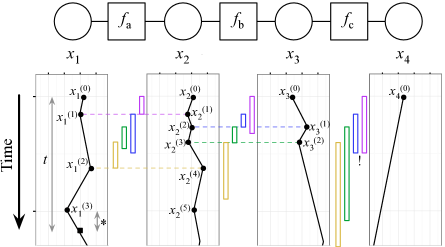
Figure 2: Top: a factor graph with $d=4$ variables and 3 binary factors, $F=\left\{f_{\text{{a}}},f_{\text{{b}}},f_{\text{{c}}}\right\}$. Bottom: sample paths of $\left(x_{i}(t)\right)_{t\geq 0}$ for $i=1,...,4$ for the local BPS. See Sections 3.2 and 3.3.1.

Such a factorization of the target density can be formalized using factor graphs (Figure 2, top). A factor graph is a bipartite graph, with one set of vertices $N$ called the variables, each corresponding to a component of $x$ ($|N|=d$), and a set of vertices $F$ corresponding to the local factors $\left(\gamma_{f}\right)_{f\in F}$. There is an edge between $k\in N$ and $f\in F$ if and only if $k\in N_{f}.$ This representation generalizes undirected graphical models [32, Chap. 2, Section 2.1.3] as, for example, factor graphs can have distinct factors connected to the same set of components (i.e. $f\neq f^{\prime}$ with $N_{f}=N_{f^{\prime}}$) as in the example of Section 4.6.

3.2 Local BPS: algorithm description

Similarly to the Gibbs sampler, each step of the local BPS manipulates only a subset of the $d$ components of $x$. Contrary to the Gibbs sampler, the local BPS does not require sampling from any full conditional distribution and each local calculation results in a change of all state components, not just the one being updated—how this can be done implicitly without manipulating the full state at each iteration is described below. Related processes exhibiting similar characteristics have been proposed in [19, 22, 23, 25].

For each factor $f\in F$, we define a local intensity function $\lambda_{f}:\mathbb{R}^{d}\times\mathbb{R}^{d}\rightarrow\mathbb{R}^{+}$ and a local bouncing matrix $R_{f}:\mathbb{R}^{d}\rightarrow\mathbb{R}^{d\times d}$ by

$$\lambda_{f}\left(x,v\right) =\mathrm{max}\left\{0,\left\langle\nabla U_{f}\left(x\right),v\right\rangle\right\},$$ (17)

$$R_{f}\left(x\right)v =v-2\frac{\left\langle\nabla U_{f}\left(x\right),v\right\rangle\nabla U_{f}\left(x\right)}{\left\|\nabla U_{f}\left(x\right)\right\|^{2}}.$$ (18)

We can check that $R_{f}\left(x\right)$ satisfies

$$k\in\left\{1,2,\dots,d\right\}\backslash N_{f}\Longrightarrow\{R_{f}(x)v\}_{k}=v_{k}.$$ (19)

When suitable, we will slightly abuse notation and write $R_{f}\left(x_{f}\right)$ for $R_{f}\left(x\right)$ as $R_{f}\left(x_{f},x_{-f}\right)=R_{f}\left(x_{f},x^{\prime}_{-f}\right)$ for any $x_{-f},x^{\prime}_{-f}\in\mathbb{R}^{d-\left|N_{f}\right|}$, where $\left|S\right|$ denotes the cardinality of a set $S$. Similarly, we will use $\lambda_{f}(x_{f},v_{f})$ for $\lambda_{f}(x,v)$.

We define a collection of PP intensities based on the previous event position $x^{(i-1)}$ and velocity $v^{(i-1)}$: $\chi_{f}(t)=\lambda_{f}(x^{\left(i-1\right)}+v^{\left(i-1\right)}t,v^{\left(i-1\right)})$. In the local BPS, the next bounce time $\tau$ is the first arrival of a PP with intensity $\chi(t)=\sum_{f\in F}\chi_{f}(t)$. However, instead of modifying all velocity variables at a bounce as in the basic BPS, we sample a factor $f$ with probability $\chi_{f}(\tau)/\chi(\tau)$ and modify only the variables connected to the sampled factor. More precisely, the velocity $v_{f}$ is updated using $R_{f}\left(x_{f}\right)$ defined in (18). A generalization of the proof of Proposition 1 given in the Supplementary Material shows that the local BPS algorithm results in a $\pi-$invariant kernel. In the next subsection, we describe various computationally efficient procedures to simulate this process.

For all these implementations, it is useful to encode trajectories in a sparse fashion: each variable $k\in N$ only records information at the times $t_{k}^{(1)},t_{k}^{(2)},\dots$ where an event (a bounce or refreshment) affected it. By (19), this represents a sublist of the list of all event times. At each of those times $t_{k}^{(i)},$ the component’s position $x_{k}^{(i)}$ and velocity $v_{k}^{(i)}$ right after the event is stored. Let $L_{k}$ denote a list of triplets $(x_{k}^{(i)},v_{k}^{(i)},t_{k}^{(i)})_{i\geq 0}$, where $x_{k}^{(0)}$ and $v_{k}^{(0)}$ denote the initial position and velocity and $t_{k}^{(0)}=0$ (see Figure 2, where the black dots denote the set of recorded triplets). This list is sufficient to compute $x_{k}(t)$ for $t\leq t_{k}^{(|L_{k}|+1)}$. This procedure is detailed in Algorithm 3 and an example is shown in Figure 2, where the black square on the first variable’s trajectory shows how Algorithm 3 reconstructs $x_{1}(t)$ at a fixed time $t$: it identifies $i(t,1)=3$ as the index associated to the largest event time $t_{1}^{(3)}$ before time $t$ affecting $x_{1}$ and return $x_{1}\left(t\right)=x_{1}^{(3)}+v_{1}^{(3)}(t-t_{1}^{(3)})$.

Algorithm 3 Computation of $x_{k}(t)$ from a list of events.  

1. Find the index $i=i(t,k)$ associated to the largest time $t_{k}^{(i)}$ verifying $t_{k}^{(i)}\leq t$.

2. Set $x_{k}(t)\leftarrow x_{k}^{(i(t,k))}+(t-t_{k}^{(i(t,k))})v_{k}^{(i(t,k))}.$

3.3 Local BPS: efficient implementations

3.3.1 Implementation via priority queue

We can sample arrivals from a PP with intensity $\chi(t)=\sum_{f\in F}\chi_{f}(t)$ using the superposition method of Section 2.3.3, the thinning step therein being omitted. To implement this technique efficiently, we store potential future bounce times (called “candidates”) $t_{f}$, one for each factor, in a priority queue $Q$: only a subset of these candidates will join the lists $L_{k}$ which store past, “confirmed” events. We pick the the smallest time in $Q$ to determine the next bounce time and the next factor $f$ to modify. The priority queue structure ensures that finding the minimum element of $Q$ or inserting/updating an element of $Q$ can be performed with computational complexity $O(\log|F|)$. When a bounce occurs, a key observation behind efficient implementation of the local BPS is that not all the other candidate bounce times need to be resimulated. Suppose that the bounce was associated with factor $f$. In this case, only the candidate bounce times $t_{f^{\prime}}$ corresponding to factors $f^{\prime}$ with $N_{f^{\prime}}\cap N_{f}\neq\emptyset$ need to be resimulated. For example, consider the first bounce in Figure 2 (shown in purple), which is triggered by factor $f_{\text{a}}$ (rectangles represent candidate bounce times $t_{f}$; dashed lines connect bouncing factors to the variables that undergo an associated velocity change). Then only the velocities for the variables $x_{1}$ and $x_{2}$ need to be updated. Therefore, only the candidate bounce times for factors $f_{\text{a}}$ and $f_{\text{b}}$ need to be re-simulated while the candidate bounce time for $f_{\text{c}}$ stays constant (this is shown by an exclamation mark in Figure 2).

The method is detailed in Algorithm 4. Several operations of the BPS such as step 4, 6.iii, 6.iv and 7.ii can be easily parallelized.

Algorithm 4 Local BPS algorithm (priority queue implementation)  

1. Initialize $\left(x^{\left(0\right)},v^{\left(0\right)}\right)$ arbitrarily on $\mathbb{R}^{d}\times\mathbb{R}^{d}$.

2. Initialize the global clock $T\leftarrow 0$.

3. For $k\in N$ do

   1. Initialize the list $L_{k}\leftarrow\left(x_{k}^{\left(0\right)},v_{k}^{\left(0\right)},T\right)$.

4. Set $Q\leftarrow\mathbf{new\ queue}\left(x^{\left(0\right)},v^{\left(0\right)},T\right)$.

5. Sample $t_{\mathrm{ref}}\sim\mathrm{Exp\left(\lambda^{\mathrm{ref}}\right)}$.

6. While more events $i=1,2,\ldots$ requested do

   1. $\left(t,f\right)\leftarrow\mathbf{smallest\ candidate\ bounce\ time}\ \mathbf{and\ associated\ factor\ in}\ Q$.

   2. Remove $(t,f)$ from $Q$.

   3. Update the global clock, $T\leftarrow t$.

   4. If $T<t_{\mathrm{ref}}$ then

      1. $\left(v_{f}\right)_{k}\leftarrow v_{k}^{(|L_{k}|-1)}$ for all $k\in N_{f}$.

      2. $x_{f}\leftarrow x_{f}(T)$ (computed using Algorithm 3).

      3. For $k\in N_{f}$  do

         1. $x_{k}^{\left(\left|L_{k}\right|\right)}\leftarrow x_{k}^{(\left|L_{k}\right|-1)}+(T-t_{k}^{(\left|L_{k}\right|-1)})v_{k}^{(\left|L_{k}\right|-1)}$, where $t_{k}^{(\left|L_{k}\right|-1)}$ and $v_{k}^{(\left|L_{k}\right|-1)}$ are retrieved from $L_{k}$.

         2. $v_{k}^{\left(\left|L_{k}\right|\right)}\leftarrow\left\{R_{f}\left(x_{f}\right)v_{f}\right\}_{k}$.

         3. $L_{k}\leftarrow\left\{L_{k},\left(x_{k}^{\left(\left|L_{k}\right|\right)},v_{k}^{\left(\left|L_{k}\right|\right)},T\right)\right\}$ (add the new sample to the list).

      4. For $f^{\prime}\in F:N_{f^{\prime}}\cap N_{f}\neq\emptyset$ (note: this includes the update of $f$) do

         1. for all $k\in N_{f^{\prime}}$.

         2. $x_{f^{\prime}}\leftarrow x_{f^{\prime}}(T)$ (computed using Algorithm 3).

         3. Simulate the first arrival time $\tau_{f^{\prime}}$ of a PP of intensity $\lambda_{f^{\prime}}\left(x_{f^{\prime}}+tv_{f^{\prime}},v_{f^{\prime}}\right)$ on $\left[0,+\infty\right)$.

         4. Set in $Q$ the candidate bounce time associated to $f^{\prime}$ to the value $t_{f^{\prime}}=T+\tau_{f^{\prime}}$ .

   5. Else

      1. Sample $v^{\prime}\sim\mathcal{N}\left(0_{d},I_{d}\right)$.

      2. $Q\leftarrow\mathbf{new\ queue}\left(x\left(t_{\mathrm{ref}}\right),v^{\prime},t_{\mathrm{ref}}\right)$ where $x\left(t_{\mathrm{ref}}\right)$ is computed using Algorithm 3.

      3. Set $t_{\mathrm{ref}}\leftarrow t_{\mathrm{ref}}+\tau_{\mathrm{ref}}$ where $\tau_{\mathrm{ref}}\sim\mathrm{Exp\left(\lambda^{\mathrm{ref}}\right)}$.

7. Return the samples encoded as the lists $L_{k},$ $k\in N$.

Algorithm 5 New Queue $\left(x,v,T\right)$  

1. For $f\in F$ do

   1. $\left(v_{f}\right)_{k}\leftarrow v_{k}^{(|L_{k}|-1)}$ for all $k\in N_{f}$.

   2. $x_{f}\leftarrow x_{f}(T)$ (computed using Algorithm 3).

   3. Simulate the first arrival time $\tau_{f}$ of a PP of intensity $\lambda_{f}\left(x_{f}+tv_{f},v_{f}\right)$ on $\left[0,+\infty\right)$.

   4. Set in $Q$ the time associated to $f$ to the value $T+\tau_{f}$ .

2. Return $Q$.

3.3.2 Implementation via thinning

When the number of factors involved in Step 6(d)iv is large, the previous queue-based implementation can be computationally expensive. Implementing the local BPS in this setup is closely related to the problem of simulating stochastic chemical kinetics and innovative solutions have been proposed in this area. We adapt here the algorithm proposed in [31] to the local BPS context. For ease of presentation, we present the algorithm without refreshment and only detail the simulation of the bounce times. This algorithm relies on the ability to compute local-in-time upper bounds on $\lambda_{f}$ for all $f\in F$. More precisely, we assume that given a current position $x$ and velocity $v$, and $\Delta\in(0,\infty]$, we can find a positive number $\bar{\chi}_{f}$, such that for any $t\in[0,\Delta)$, we have $\bar{\chi}_{f}\geq\lambda_{f}(x+vt,v)$. We can also use this method on a subset $G$ of $F$ and combine it with the previously discussed techniques to sample candidate bounce times for factors in $F$\$G$ but we restrict ourselves to $G=F$ to simplify the presentation.

Algorithm 6 Local BPS algorithm (thinning implementation)  

1. Initialize $\left(x^{\left(0\right)},v^{\left(0\right)}\right)$ arbitrarily on $\mathbb{R}^{d}\times\mathbb{R}^{d}$.

2. Initialize the global clock $T\leftarrow 0$.

3. Initialize $\bar{T}\leftarrow\triangle$ (time until which local upper bounds are valid).

4. Compute local-in-time upper bounds $\bar{\chi}_{f}$ for $f\in F$ such that $\bar{\chi}_{f}\geq\lambda_{f}(x^{(0)}+v^{(0)}t,v^{\left(0\right)})$ for all $t\in[0,\Delta)$.

5. While more events $i=1,2,\ldots$ requested do

   1. Sample $\tau\sim\mathrm{Exp\left(\bar{\chi}\right)}$ where $\bar{\chi}=\sum_{f\in F}\bar{\chi}_{f}$.

   2. If $\left(T+\tau>\bar{T}\right)$ then

      1. $x^{(i)}\leftarrow x^{(i-1)}+v^{(i-1)}(\bar{T}-T)$.

      2. $v^{(i)}\leftarrow v^{(i-1)}$.

      3. For all $f\in F$, update $\bar{\chi}_{f}$ to ensure that $\bar{\chi}_{f}\geq\lambda_{f}(x^{(i)}+v^{(i)}t,v^{(i)})$ for $t\in[0,\Delta)$.

      4. Set $T\leftarrow\bar{T}$, $\bar{T}$$\leftarrow\bar{T}+\triangle.$

   3. Else

      1. $x^{(i)}\leftarrow x^{(i-1)}+v^{(i-1)}\tau$.

      2. Sample $\mathcal{F}\in F$ where $\mathbb{P}\left(\mathcal{F}=f\right)=\bar{\chi}_{f}/\bar{\chi}.$

      3. If $V<\lambda_{\mathcal{F}}\left(x^{(i)},v^{(i-1)}\right)/\bar{\chi}_{\mathcal{F}}$ where $V\sim\mathcal{U}\left(0,1\right)$ then a bounce for factor $\mathcal{F}$ occurs at time $T$.

         1. $v^{(i)}$$\leftarrow R_{\mathcal{F}}\left(x^{(i)}\right)v^{(i-1)}$.

         2. For all $f^{\prime}\in F:N_{f^{\prime}}\cap N_{\mathcal{F}}\neq\emptyset$, update $\bar{\chi}_{f^{\prime}}$ to ensure that $\bar{\chi}_{f^{\prime}}\geq\lambda_{f^{\prime}}(x^{(i)}+v^{(i)}t,v^{(i)})$ for $t\in[0,\bar{T}-T-\tau)$.

      4. Else

         1. $v^{(i)}\leftarrow v^{(i-1)}$.

      5. Set $T\leftarrow T+\tau$.

Algorithm 6 will be particularly useful in scenarios where summing over the bounds (Step 5a) and sampling a factor (Step 5(c)ii) can be performed efficiently. A scenario where it is possible to implement these two operations in constant time is detailed in Section 4.6. Another scenario where sampling quickly from $\mathcal{F}$ is feasible is if the number of distinct upper bounds is much smaller than the number of factors. For example, we only need to sample a factor $\mathcal{F}$ uniformly at random if $\Lambda=\bar{\chi}_{f}=\bar{\chi}_{f^{\prime}}$ for all $f,f^{\prime}$ in $F$ and $\bar{\chi}=\left|F\right|\cdot\Lambda$ (that is no factor needs to be inspected in order to execute Algorithm 5(c)ii) and the thinning procedure in Step 5(c)iii boils down to

$$V\leq\frac{\left|F\right|\max\left(0,\left\langle\nabla U_{f}(x^{(i)}),v^{\left(i-1\right)}\right\rangle\right)}{\bar{\chi}}.$$ (20)

A related approach has been adopted in [4] for the analysis of big data. In this particular scenario, an alternative local BPS can also be implemented where $s>1$ factors $\mathcal{F}=\left(\mathcal{F}_{1},\dots,\mathcal{F}_{s}\right)$ are sampled uniformly at random without replacement from $F$, the thinning occurs with probability

$$\frac{\left|F\right|}{s\bar{\chi}}\max\left(0,\sum_{j=1}^{s}\left\langle\nabla U_{\mathcal{F}_{j}}(x^{(i)}),v^{\left(i-1\right)}\right\rangle\right)$$ (21)

and the components of $x$ belonging to $N_{\mathcal{F}}$ bounce based on $\sum_{j=1}^{s}\nabla U_{\mathcal{F}_{j}}(x)$. One can check that the resulting dynamics preserves $\pi$ as an invariant distribution. In contrast to $s=1$, this is not an implementation of local BPS described in Algorithm 6, but instead this corresponds to a local BPS update for a random partition of the factors.

4 Numerical results

4.1 Gaussian distributions and the need for refreshment

We consider an isotropic multivariate Gaussian target distribution, $U\left(x\right)=\left\|x\right\|^{2}$, to illustrate the need for refreshment. Without refreshment, we obtain from Equation (7)

$$\left\langle x^{(i)},v^{(i)}\right\rangle = \begin{cases}-\sqrt{-\log V_{i}}&\text{if }\left\langle x^{(i-1)},v^{(i-1)}\right\rangle\leq 0,\\ -\sqrt{\left\langle x^{(i-1)},v^{(i-1)}\right\rangle^{2}-\log V_{i}}&\text{otherwise,}\end{cases}$$

and

$$\left\|x^{(i)}\right\|^{2}=\begin{cases}\left\|x^{(i-1)}\right\|^{2}-\left\langle x^{(i-1)},v^{(i-1)}\right\rangle^{2}-\log V_{i}&\text{ if }\left\langle x^{(i-1)},v^{(i-1)}\right\rangle\leq 0,\\ \left\|x^{(i-1)}\right\|^{2}-\log V_{i}&\text{otherwise,}\end{cases}$$

see Supplementary Material for details. In particular, these calculations show that if $\left\langle x^{(i)},v^{(i)}\right\rangle\leq 0$ then $\left\langle x^{(j)},v^{(j)}\right\rangle\leq 0$ for $j>i$ so that $\|x^{(i)}\|^{2}=\left\|x^{(1)}\right\|^{2}-\left\langle x^{(1)},v^{(1)}\right\rangle^{2}-\log V_{i}$ for $i\geq 2$. In particular for $x^{(0)}=e_{1}$ and $v^{(0)}=e_{2}$ with $e_{i}$ being elements of standard basis of $\mathbb{R}^{d}$, the norm of the position at all points along the trajectory can never be smaller than $1$ as illustrated in Figure 3.

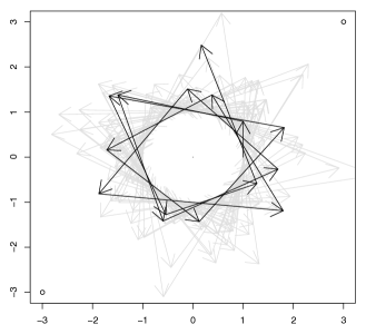
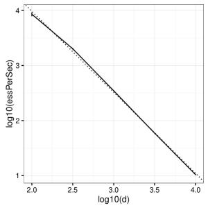
Figure 3: Left: the 200 first segments/bounces of a BPS path for $\lambda^{\mathrm{ref}}=0$ (for clarity the first 15 segments are in black, the following ones in light grey): the center of the space is never explored. Right, solid line: ESS per CPU second as a function of $d$ (log-log scale), along with 95% confidence intervals based on 40 runs (the intervals are small and difficult to see). Dashed line: linear regression curve. See Section 4.1 for details.

In this scenario, we show that BPS without refreshment admits a countably infinite collection of invariant distributions. Let us define $r\left(t\right)=\left\|x\left(t\right)\right\|$ and $m\left(t\right)=\left\langle x\left(t\right),v\left(t\right)\right\rangle/\left\|x\left(t\right)\right\|$ and denote by $\chi_{k}$ the probability density of the chi distribution with $k$ degrees of freedom.

Proposition 2.

For any dimension $d\geq 2$, the process $\left(r\left(t\right),m\left(t\right)\right)_{t\geq 0}$ is Markov and its transition kernel is invariant with respect to the probability densities $\left\{f_{k}(r,m)\propto\chi_{k}(\sqrt{2}r)\cdot(1-{\Hy@raisedlink{\hypertarget{xv}{}}{m}}^{2})^{(k-3)/2};k\in\left\{2,3,\ldots\right\}\right\}$.

The proof is given in Appendix 2. By Theorem 1, we have a unique invariant measure as soon as $\lambda^{\mathrm{ref}}>0$.

Next, we look at the scaling of the Effective Sample Size (ESS) per CPU second of the basic BPS algorithm for $\varphi\left(x\right)=x_{1}$ when $\lambda_{\text{ref}}=1$ as the dimension $d$ of the isotropic normal target increases. The ESS is estimated using the R package mcmcse [10] by evaluating the trajectory on a fine discretization of the sampled trajectory. The results in log-log scale are displayed in Figure 3. The curve suggests a decay of roughly $d^{-1.47}$, slightly inferior to the $d^{-1.25}$ scaling for an optimally tuned Hamiltonian Monte Carlo (HMC) algorithm [6, Section III], [24, Section 5.4.4]. It should be noted that BPS achieves this scaling without varying any tuning parameter, whereas HMC’s performance critically depends on tuning two parameters (leap-frog stepsize and number of leap-frog steps). Both BPS and HMC compare favorably to the $d^{-2}$ scaling of the optimally tuned random walk MH [28].

4.2 Comparison of the global and local schemes

We compare the basic “global” BPS of Section 2 to the local BPS of Section 3 on a sparse Gaussian field. We use a chain-shaped undirected graphical model of length $d=1000$ and perform separate experiments for various pairwise precision parameters for the interaction between neighbors in the chain. Both methods are run for 60 seconds. We compare the Monte Carlo estimate of the variance of $x_{500}$ to its true value. The results are shown in Figure 4. The smaller computational complexity per local bounce of the local BPS offsets significantly the associated decrease in expected trajectory segment length. Moreover, both versions appear insensitive to the pairwise precision used in this sparse Gaussian field.

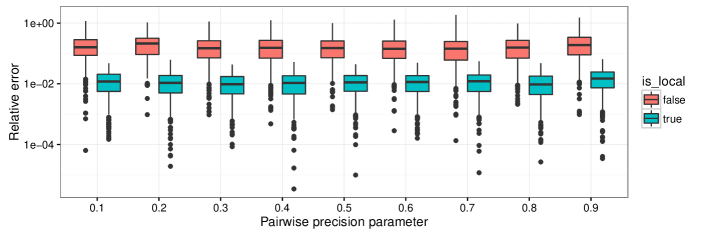
Figure 4: Boxplots of relative errors over 100 local BPS runs for Gaussian chain-shaped fields of pairwise precisions 0.1-0.9 .

4.3 Comparisons of alternative refreshment schemes

In Section 2, the velocity was refreshed using a Gaussian distribution. We compare here this global refreshment scheme to three alternatives:

Local refreshment:

if the local BPS is used, the factor graph structure can be exploited to design computationally cheaper refreshment operators. We pick one factor $f\in F$ uniformly at random and resample only the components of $v$ with indices in $N_{f}$. By the same argument used in Section 3, each refreshment requires bounce time recomputation only for the factors $f^{\prime}$ with $N_{f}\cap N_{f^{\prime}}\neq\emptyset$.

Restricted refreshment:

the velocities are refreshed according to $\phi\left(v\right)$, the uniform distribution on $\mathcal{S}^{d-1}$, and the BPS admits now $\rho\left(z\right)=\pi\left(x\right)\phi\left(v\right)$ as invariant distribution.

Restricted partial refreshment:

a variant of restricted refreshment where we sample an angle $\theta$ by multiplying a Beta($\alpha$, $\beta$)-distributed random variable by $2\pi.$ We then select a vector uniformly at random from the unit length vectors that have an angle $\theta$ from $v$. We used $\alpha=1,\beta=4$ to favor small angles.

We compare these methods for different values of $\lambda^{\mathrm{ref}}$, the trade-off being that too small a value can lead to a failure to visit certain regions of the space, while too large a value leads to a random walk behavior.

The rationale behind the partial refreshment procedure is to suppress the random walk behavior of the particle path arising from a refreshment step independent from the current velocity. Refreshment is needed to ensure ergodicity but a “good” direction should only be altered slightly. This strategy is akin to the partial momentum refreshment strategy for HMC methods [17], [24, Section 4.3] and could be similarly implemented for global refreshment. It is easy to check that all of the above schemes preserve $\pi$ as invariant distribution. We tested these schemes on the chain-shaped factor graph described in the previous section (with the pairwise precision parameter set to 0.5). All methods are provided with a computational budget of 30 seconds. The results are shown in Figure 5. The results show that local refreshment is less sensitive to $\lambda^{\mathrm{ref}}$, performing as well or better than global refreshment. The performance of the restricted and partial methods appears more sensitive to $\lambda^{\mathrm{ref}}$ and generally inferior to the other two schemes.

One limitation of the results in this section is that the optimal refreshment scheme and refreshment rate will in general be problem dependent. Adaptation methods used in the HMC literature could potentially be adapted to this scenario [33, 16], but we leave these extensions to future work.

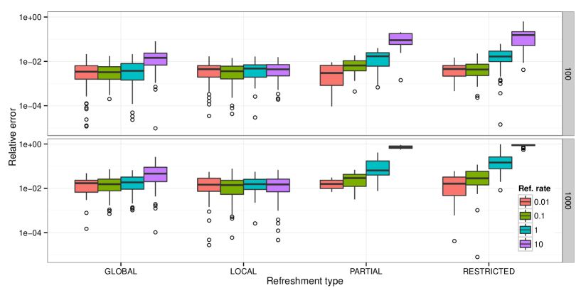
Figure 5: Comparison of refreshment schemes for $d=100$ (top) and $d=1000$ (bottom). Each boxplot summarizes the relative error for the variance estimates (in log scale) of $x_{50}$ over 100 runs of BPS.

4.4 Comparisons with HMC methods on high-dimensional Gaussian distributions

We compare the local BPS with no partial refreshment and $\lambda^{\mathrm{ref}}=1$ to advanced adaptive versions of HMC implemented using Stan [16] on a 100-dimensional Gaussian example from [24, Section 5.3.3.4]. For each method, we compute the relative error on the estimated marginal variances after a wall clock time of 30 seconds, excluding from this time the time taken to compile the Stan program. The adaptive HMC methods use 1000 iterations of adaptation. When only the leap-frog stepsize is adapted (“adapt=true”), HMC provides several poor estimates of marginal variances. These deviations disappear when adapting a diagonal metric (denoted “fit-metric”) and/or using advanced auxiliary variable methods to select the number of leap-frog steps (denoted “nuts”). Given that adaptation is critical to HMC in this scenario, it is encouraging that BPS without adaptation is competitive (Figure 6).

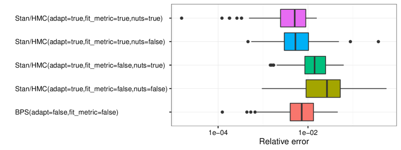
Figure 6: Box plots showing the relative absolute error of variance estimates for a fixed computational budget.

Next, we compare the local BPS to NUTS (“adapt=true,fit_metric=true,nuts=true”) as the dimension $d$ increases. Experiments are performed on the chain-shaped Gaussian Random Field of Section 4.2 with the pairwise precision parameter set to 0.5. We vary the length of the chain (10, 100, 1000), and run Stan’s implementation of NUTS for 1000 iterations + 1000 iterations of adaptation. We measure the wall-clock time (excluding the time taken to compile the Stan program) and then run our method for the same wall-clock time 40 times for each chain size. The absolute value of the relative error averaged on 10 equally spaced marginal variances is measured as a function of the percentage of the total computational budget used; see Figure 7. The gap between the two methods widens as $d$ increases. To visualize the different behavior of the two algorithms, three marginals of the Stan and BPS paths for $d=100$ are shown in Figure 8. Contrary to Section 4.1, BPS outperforms here HMC as its local version is able to exploit the sparsity of the random field.

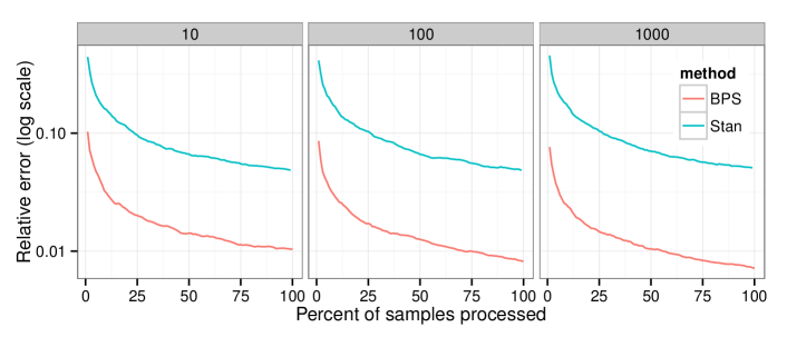
Figure 7: Relative error for $d=10$ (left), $d=100$ (middle) and $d=1000$ (right), averaged over 10 of the dimensions and 40 runs. Each $d$ uses a fixed computational budget.

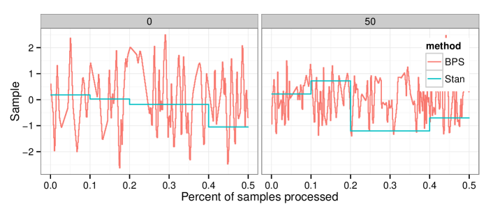
Figure 8: Simulated paths for $x_{0}$ and $x_{50}$ for $d=100$. Each state of the HMC trajectory is obtained by leap-frog steps (not displayed), these latter cannot be used to estimate Monte Carlo averages as HMC relies on a MH step. In contrast, BPS exploits the full path.

4.5 Poisson-Gaussian Markov random field

Let $x=(x_{i,j}:i,j\in\left\{1,2,\dots,10\right\})$ denote a grid-shaped Gaussian Markov random field with pairwise interactions of the same form as those used in the previous chain examples (pairwise precision set to 0.5) and let $y_{i,j}$ be Poisson distributed, independent over $i,j$ given $x$, with rate $\exp(x_{i,j})$. We generate a synthetic dataset $y=(y_{i,j}:i,j\in\left\{1,2,\dots,10\right\})$ from this model and approximate the resulting posterior distribution of $x$. We first run Stan with default settings (“adapt=true,fit_metric=true,nuts=true”) for $16,32,64,\dots,4096$ iterations. For each number of Stan iterations, we run local BPS for the same wall-clock time as Stan, using a local refreshment ($\lambda^{\mathrm{ref}}=1$) and the method from Example 2 for the bouncing time computations. We repeat these experiments 10 times with different random seeds. Figure 9 displays the boxplots of the estimates of the posterior variances of the variables $x_{0,0}$ and $x_{5,5}$ summarizing the 10 replications. As expected, both methods converge to the same value, but BPS requires markedly less computing time to achieve any given level of accuracy.

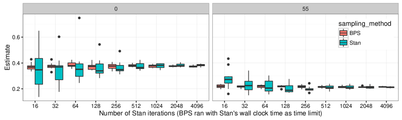
Figure 9: Boxplots of estimates of the posterior variance of $x_{0,0}$ (left) and $x_{5,5}$ (right) using Stan implementation of HMC and local BPS.

4.6 Bayesian logistic regression for large data sets

Consider the logistic regression model introduced in Example 3 when the number of data $R$ is large. In this context, standard MCMC schemes such as the MH algorithm are computationally expensive as they require evaluating the likelihood associated to the $R$ observations at each iteration. This has motivated the development of techniques which only evaluate the likelihood of a subset of the data at each iteration. However, most of the methods currently available introduce either some non-vanishing asymptotic bias, e.g. the subsampling MH scheme proposed in [2], or provide consistent estimates converging at a slower rate than regular MCMC algorithms, e.g. the Stochastic Gradient Langevin Dynamics introduced in [34, 30]. The only available algorithm which only requires evaluating the likelihood of a subset of data at each iteration yet provides consistent estimates converging at the standard Monte Carlo rate is the Firefly algorithm [21].

In this context, we associate $R+1$ factors to the target posterior distribution: one for the prior and one for each data point with $x_{f}=x$ for all $f\in F$. As a uniform upper bound on the intensities of these local factors is available for restricted refreshment, see Appendix C.1, we could use (21) in conjunction with Algorithm 6 to provide an alternative to the Firefly algorithm which selects at each bounce a subset of $s$ data points uniformly at random without replacement. For $s=1$, a related algorithm has been recently explored in [4]. In presence of outliers, this strategy can be inefficient as the uniform upper bound becomes very large, resulting in a computationally expensive implementation. After a pre-computation step of complexity $O(R\log R)$ only executed once, we show here that Algorithm 6 can be implemented using data-dependent bounds mitigating the sensitivity to outliers while maintaining the computational cost of each bounce independent of $R$. We first pre-compute the sum of covariates over the data points, $\iota_{k}^{c}=\sum_{r=1}^{R}\iota_{r,k}{\mathbf{1}}[y_{r}=c]$, for $k\in\left\{1,\ldots,d\right\}$ and class label $c\in\left\{0,1\right\}$. Using these quantities, it is possible to compute

$$\bar{\chi} =\sum_{r=1}^{R}\bar{\chi}^{[r]}=\sum_{k=1}^{d}|v_{k}|\ \iota_{k}^{{\mathbf{1}}[v_{k}<0]},$$

with $\bar{\chi}^{[r]}$ given in (12). If $d$ is large, we can keep the sum $\bar{\chi}$ in memory and add-and-subtract any local updates to it. The implementation of Step 5(c)ii relies on the alias method [8, Section 3.4]. A detailed description of these derivations and of the algorithm is presented in Appendix C.

We compare the local BPS with thinning to the MAP-tuned Firefly algorithm implementation provided by the authors. This version of Firefly outperforms experimentally significantly the standard MH in terms of ESS per-datum likelihood [21]. The two algorithms are here compared in terms of this criterion, where the ESS is averaged over the $d=5$ components of $x$. We generate covariates $\iota_{rk}\overset{\text{i.i.d.}}{\sim}\mathcal{U}(0.1,1.1)$ and data $y_{r}\in\{0,1\}$ for $r=1,\dots,R$ according to (9) and set a zero-mean normal prior of covariance $\sigma^{2}I_{d}$ for $x$. For the algorithm, we set $\lambda_{\text{ref}}=0.5,\,\sigma^{2}=1$ and $\Delta=0.5$, which is the length of the time interval for which a constant upper bound for the rate associated with the prior is used, see Algorithm 7. Experimentally, local BPS always outperforms Firefly, by about an order of magnitude for large data sets. However, we also observe that both Firefly and local BPS have an ESS per datum likelihood evaluation decreasing in approximately $1/R$ so that the gains brought by these algorithms over a correctly scaled random walk MH algorithm do not appear to increase with $R$. The rate for local BPS is slightly superior in the regime of up to $10^{4}$ data points, but then returns to the approximate $1/R$ rate. To improve this rate, one can adapt the control variate ideas introduced in [3] for the MH algorithm to these schemes. This has been proposed in [4] for a related algorithm and in [11] for the local BPS.

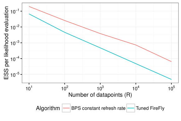
Figure 10: ESS per-datum likelihood evaluation for Local BPS and Firefly.

4.7 Bayesian inference of evolutionary parameters

We analyze a dataset of primate mitochondrial DNA [15] at the leaves of a fixed reference tree [18] containing 898 sites and 12 species. We want to approximate the posterior evolutionary parameters $x$ encoded into a rate matrix $Q$. A detailed description of this phylogenetic model can be found in the Supplementary Material. The global BPS is used with restricted refreshment and $\lambda^{\mathrm{ref}}=1$ in conjunction with an auxiliary variable-based method similar to the one described in [35], alternating between two moves: (1) sampling continuous-time Markov chain paths along the tree given $x$ using uniformization, (2) sampling $x$ given the path (in which case the derivation of the gradient is simple and efficient). The only difference compared to [35] is that we substitute the HMC kernel by the kernel induced by running BPS for a fixed trajectory length. This auxiliary variable method is convenient because, conditioned on the paths, the energy function is convex and hence we can simulate the bouncing times using the method described in Example 1.

We compare against a state-of-the-art HMC sampler [33] that uses Bayesian optimization to adapt the key parameters of HMC, the leap-frog stepsize and the number of leap-frog steps, while preserving convergence to the target distribution. Both our method and this HMC method are implemented in Java and share the same gradient computation code. Refer to the Supplementary Material for additional background and motivation behind this adaptation method.

We first perform various checks to ensure that both BPS and HMC chains are in close agreement given a sufficiently large number of iterations. After 20 millions HMC iterations, the credible intervals estimates from the HMC method are in close agreement with those obtained from BPS (result not shown) and both methods pass the Geweke diagnostic [12].

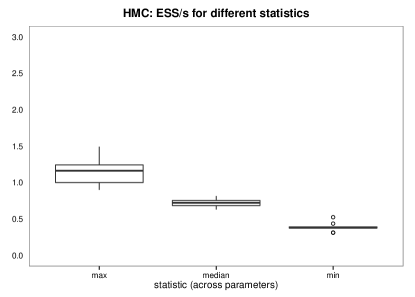
Figure 11: Boxplots of maximum, median and minimum ESS per second for BPS (left) and HMC (right).

To compare the effectiveness of the two samplers, we look at the ESS per second of the model parameters. We show the maximum, median, and maximum over the 10 parameter components for 10 runs, for both BPS and HMC in Figure 11. We observe a speed-up by a factor two for all statistics considered (maximum, median, minimum). In the supplement, we show that the HMC chain displays much larger autocorrelations than the BPS chain.

5 Discussion

Most MCMC methods currently available, such as the MH and HMC algorithms, are discrete-time reversible processes. There is a wealth of theoretical results showing that non-reversible Markov processes mix faster and provide lower variance estimates of ergodic averages [26]. However, most of the non-reversible processes studied in the literature are diffusions and cannot be simulated exactly. The BPS is an alternative continuous-time Markov process which, thanks to its piecewise deterministic paths, can be simulated exactly for many problems of interest in statistics.

As any MCMC method, the BPS can struggle in multimodal scenarios and when the target exhibits very strong correlations. However, for a range of applications including sparse factor graphs, large datasets and high-dimensional settings, we have observed empirically that BPS is on par or outperforms state-of-the art methods such as HMC and Firefly. The main practical limitation of the BPS compared to HMC is that its implementation is model-specific and requires more than knowing $\nabla U$ pointwise. An important open problem is therefore whether its implementation, and in particular the simulation of bouncing times, can be fully automated. However, the techniques described in Section 2.3 are already sufficient to handle many interesting models. There are also numerous potential methodological extensions of the method to study. In particular, it has been shown in [13] how one can exploit the local geometric structure of the target to improve HMC and it would be interesting to investigate how this could be achieved for BPS. More generally, the BPS is a specific continuous-time piecewise deterministic Markov process [7]. This class of processes deserves further exploration as it might provide a whole new class of efficient MCMC methods.

Appendix A Proofs of Section 2

A.1 Proof of Proposition 1

The BPS process is a specific piecewise-deterministic Markov process so the expression of its generator follows from [7, Theorem 26.14]. Its adjoint is given in [27] and a derivation of this expression from first principles can be found in the Supplementary Material. To establish the invariance with respect to $\rho$, we first show that $\mathcal{\int L}h(z)\rho\left(z\right){\rm d}z=0$. We have

$$\mathcal{\int\int L}h(z)\rho\left(z\right){\rm d}z = \int\int\left\langle\nabla_{x}h\left(x,v\right),v\right\rangle\rho\left(z\right){\rm d}z$$ (24)

$$+\int\int\lambda(x,v)[h\left(x,R\left(x\right)v\right)-h\left(x,v\right)]\rho\left(z\right){\rm d}z$$

$$+\lambda^{\mathrm{ref}}\int\int\int\left(h(x,v^{\prime})-h(x,v)\right)\psi\left({\rm d}v^{\prime}\right)\rho\left(z\right){\rm d}z$$

As $\rho\left(z\right)=\pi\left(x\right)\psi\left(v\right)$, the term (24) is trivially equal to zero, while a change-of-variables shows that

$$\int\int\lambda\left(x,v\right)h(x,R\left(x\right)v)\rho\left(z\right){\rm d}z=\int\int\lambda\left(x,R\left(x\right)v\right)h(x,v)\rho\left(z\right){\rm d}z$$ (25)

as $R^{-1}\left(x\right)v=R\left(x\right)v$ and$\left\|R\left(x\right)v\right\|=\left\|v\right\|$ implies $\psi\left(R\left(x\right)v\right)=\psi\left(v\right)$. Additionally, by integration by parts, we obtain as $h$ is bounded

$$\int\int\left\langle\nabla_{x}h\left(x,v\right),v\right\rangle\rho\left(z\right){\rm d}z=\int\int\left\langle\nabla U\left(x\right),v\right\rangle h\left(x,v\right)\rho\left(z\right){\rm d}z.$$ (26)

Substituting (25) and (26) into (24)-(24)-(24), we obtain

$$\int\mathcal{\int L}h(z)\rho\left(z\right){\rm d}z=\int\int[\left\langle\nabla U\left(x\right),v\right\rangle+\lambda\left(x,R\left(x\right)v\right)-\lambda\left(x,v\right)]h(x,v)\rho\left(z\right){\rm d}z.$$

Now we have

$$\int\mathcal{\int L}h(z)\rho\left(z\right){\rm d}z = \int\int[\left\langle\nabla U\left(x\right),v\right\rangle+\lambda\left(x,R\left(x\right)v\right)-\lambda\left(x,v\right)]h(x,v)\rho\left(z\right){\rm d}z.$$

$$= \int\int[\left\langle\nabla U\left(x\right),v\right\rangle+\max\{0,\left\langle\nabla U(x),R\left(x\right)v\right\rangle\}-\max\{0,\left\langle\nabla U(x),v\right\rangle\}]h(x,v)\rho\left(z\right){\rm d}z$$

$$= \int\int[\left\langle\nabla U\left(x\right),v\right\rangle+\max\{0,-\left\langle\nabla U(x),v\right\rangle\}-\max\{0,\left\langle\nabla U(x),v\right\rangle\}]h(x,v)\rho\left(z\right){\rm d}z$$

$$= 0,$$

where we have used $\left\langle\nabla U(x),R\left(x\right)v\right\rangle=-\left\langle\nabla U(x),v\right\rangle$ and $\max\{0,-f\}-\max\{0,f\}=-f$ for any $f$. The result now follows by [7, Proposition 34.7].

A.2 Proof of Theorem 1

Informally, our proof of ergodicity relies on showing that refreshments allow the process to explore the entire space of velocities and positions, ${\mathbb{R}}^{d}\times{\mathbb{R}}^{d}.$ To do so, it will be useful to condition on an event $\mathscr{E}$ on which paths are “tractable.” Since two refreshment events are sufficient to reach any given destination point, we would like to focus on such paths (only one refreshment is not sufficient since a destination point specifies both a final position and a final velocity). In particular, refreshments are simpler to analyze than bouncing events, so we would like to condition on an event on which no bouncing occurs in a time interval of interest.

To formalize this idea, we make use of the time-scale implementation of the BPS algorithm (Section 2.3.1). This allows us to express $\mathscr{E}$ in terms of simple independent events. We start by introducing some notation for the time-scale implementation of the BPS algorithm. Let $i\geq 1$ denote the index of the current event being simulated, and assume without loss of generality that $\lambda^{\text{ref}}=$1. Let $x_{0},v_{0}$ denote the initial position and velocity, while the positions and velocities at the event times, $z_{i}=(x_{i},v_{i})$, $i\in\left\{1,2,\dots\right\}$ are defined as in Algorithm 1, we use the notation $(x_{i},v_{i})$ instead of $(x^{\left(i\right)},v^{\left(i\right)})$ to slightly simplify notation. At event time $i$, we simulate three independent random variables: two exponentially distributed, $e_{i}^{\text{(bounce)}},\tau_{i}^{\text{(ref)}}\sim\text{Exp}(1)$, and one $d$-dimensional normal, $n_{i}\sim\mathcal{N}(0,I)$. The candidate time to a refreshment is given by $\tau_{i}^{\text{(ref)}}$ and the candidate time to a bounce event is defined as $\tau_{i}^{\text{(bounce)}}=\Xi_{z_{i-1}}^{-1}(e_{i}^{\text{(bounce)}})$, where $\Xi_{z}^{-1}$ is the quantile function of $\Xi_{z}(t)=\int_{0}^{t}\chi_{z}(s)\,\mathrm{d}s$, and $\chi_{x,v}(s)=\lambda(x+vs,v)$. The time to the next event is $\tau_{i}=\min\left\{\tau_{i}^{\text{(bounce)}},\tau_{i}^{\text{(ref)}}\right\}$. The random variable $n_{i}$ is only used if $\tau_{i}=\tau_{i}^{\text{(ref)}},$ otherwise the bouncing operator is used to update the velocity in a deterministic fashion.

We can now define our tractable set and establish its key properties.

Lemma 1.

Let $t>0$, and assume the initial point of the BPS, satisfies $\|x_{0}\|\leq t$, $\|v_{0}\|\leq 1$. If $\|\nabla U\|^{*}=\sup\left\{\|\nabla U(x)\|:\|x\|\leq 3t\right\}$ then the event

$$\mathscr{E} =\underbrace{\left(\tau_{1}^{\text{(ref)}}+\tau_{2}^{\text{(ref)}}\leq t<\tau_{1}^{\text{(ref)}}+\tau_{2}^{\text{(ref)}}+\tau_{3}^{\text{(ref)}}\right)}_{\mathscr{E}_{1}}\cap \underbrace{\bigcap_{i\in\left\{1,2\right\}}\left(\|n_{i}\|\leq 1\right)}_{\mathscr{E}_{2}}\cap\underbrace{\bigcap_{i\in{1,2,3}}\left(e_{i}^{\text{(bounce)}}\geq t\|\nabla U\|^{*}\right)}_{\mathscr{E}_{3}}$$

has the following properties:

1. On the event $\mathscr{E}$, we have $\|v(t^{\prime})\|\leq 1$ and $\|x(t^{\prime})\|\leq 2t$ for all $t^{\prime}\in\left[0,t\right]$,

2. On the event $\mathscr{E}$, there are exactly two refreshments and no bouncing in the interval $(0,t)$, i.e. $\tau_{1}=\tau_{1}^{\text{(ref)}}$, $\tau_{2}=\tau_{2}^{\text{(ref)}},$ and $\tau_{1}+\tau_{2}\leq t\leq\tau_{1}+\tau_{2}+\tau_{3}$,

3. ${\mathbb{P}}(\mathscr{E})$ is a strictly positive constant that does not depend on $z(0)=(x_{0},v_{0})$,

4. $v_{i}|\mathscr{E}\overset{\text{i.i.d.}}{\sim}\psi_{\leq 1}(0,I)$ for $i\in\left\{1,2\right\}$, where $\psi_{\leq 1}$ denotes the truncated Gaussian distribution, with $\|v_{i}\|\leq 1$,

5. $\left(\tau_{1}^{\text{(ref)}},\tau_{2}^{\text{(ref)}}\right)|\mathscr{E}\sim\mathcal{U}\left(\left\{(\tau_{1},\tau_{2})\in(0,t)^{2}:\tau_{1}+\tau_{2}\leq t\right\}\right)$.

Proof.

To prove Part 1 and 2, we will make use of this preliminary result: on $\mathscr{E}_{3},$ $\|v_{i-1}\|\leq 1,\|x_{i-1}\|\leq 2t$ implies $\tau_{i}^{\text{(bounce)}}\geq t$ for $i\in\left\{1,2,3\right\}$. Indeed, $\|v_{i-1}\|\leq 1$ and $\|x_{i-1}\|\leq 2t$ imply that $\chi_{z_{i-1}}(t^{\prime})\leq\|\nabla U\|^{*}$ for all $t^{\prime}\in\left[0,t\right]$. It follows that $\Xi_{z_{i-1}}(t)\leq\|\nabla U\|^{*}t$. Hence, by the continuity of $\Xi_{z_{i-1}}$ and standard properties of the quantile function, $\tau_{i}^{\text{(bounce)}}=\Xi_{z_{i-1}}^{-1}(e_{i}^{\text{(bounce)}})\geq t$.

Part 1 and 2: by the assumption on $x_{0}$ and $v_{0}$ and our preliminary result, $\tau_{1}^{\text{(bounce)}}\geq t$, and hence, combining with $\mathscr{E}_{1}$ and $\mathscr{E}_{2}$ we have $\tau_{1}=\tau_{1}^{\text{(ref)}}\leq t$ and $\|v_{1}\|=\|n_{1}\|\leq 1$. Also, by the triangle inequality, $\|x_{1}\|\leq\|x_{0}\|+\|x_{1}-x_{0}\|\leq t+\tau_{1}^{\text{(ref)}}\leq 2t$. We can therefore apply our preliminary result again and obtain $\tau_{2}^{\text{(bounce)}}\geq t$, and hence, combining again with $\mathscr{E}_{1}$ and $\mathscr{E}_{2}$, we have $\tau_{2}=\tau_{2}^{\text{(ref)}}$, $\tau_{1}+\tau_{2}\leq t$, $\|v_{2}\|=\|n_{2}\|\leq 1$. Applying the triangle inequality a second time yields $\|x_{2}\|\leq t+\tau_{1}^{\text{(ref)}}+\tau_{2}^{\text{(ref)}}\leq 2t$. We apply our preliminary result one last time to obtain $\tau_{3}^{\text{\text{(bounce)}}}\geq t$. Hence, if $\tau_{3}^{\text{(ref)}}>\tau_{3}^{\text{(bounce)}}$, $\tau_{1}+\tau_{2}+\tau_{3}=\tau_{1}^{\text{(ref)}}+\tau_{2}^{\text{(ref)}}+\tau_{3}^{\text{(bounce)}}\geq t$, while if $\tau_{3}^{\text{(ref)}}\leq\tau_{3}^{\text{(bounce)}}$, we can use $\mathscr{E}_{1}$ to conclude that $\tau_{1}+\tau_{2}+\tau_{3}=\tau_{1}^{\text{(ref)}}+\tau_{2}^{\text{(ref)}}+\tau_{3}^{\text{(ref)}}\geq t$. It follows from the triangle inequality that $\|x(t^{\prime})\|\leq 2t$ for all $t^{\prime}\in\left[0,t\right]$.

Part 3, 4 and 5: these follow straightforwardly from the construction of $\mathscr{E}$. ∎

Note that the statement and proof of Part 4 is simple because $\mathscr{E}_{3}\in\sigma(e_{i}^{\text{(bounce)}}:i\in\left\{1,2,3\right\})$. In contrast, conditioning on conceptually simpler events of the form $(\tau_{i}^{\text{(bounce)}}>t)\in\sigma\left(e_{i}^{\text{(bounce)}},z_{i-1}\right)$ leads to conditional distributions on $v_{k}$ which are harder to characterize.

In the following, $B_{R}\left(x\right)$ denotes the $d$-dimensional Euclidean ball of radius $R$ centered at $x$.

Lemma 2.

For all $\epsilon,t>0$ such that $\epsilon\leq t/6$, and $v,v_{2}\in B_{1}(0)$, $x,x^{\prime}\in B_{\epsilon}(0)$, $0\leq\tau_{1}\leq\frac{t}{6}$, and $\frac{2t}{3}\leq\tau_{2}\leq\frac{5t}{6}$, we have $\left\|v_{1}\right\|\leq 1$, where $v_{1}$ is defined by:

$$v_{1}=\frac{\left(x^{\prime}-(t-\tau_{1}-\tau_{2})v_{2}\right)-\left(x+\tau_{1}v\right)}{\tau_{2}}.$$ (27)

Proof.

By the triangle inequality:

$$\|v_{1}\| \leq \frac{\|x^{\prime}\|+(t-\tau_{1}-\tau_{2})\|v_{2}\|+\|x\|+\tau_{1}\|v\|}{\tau_{2}}$$

$$\leq \frac{\epsilon+(t-\tau_{1}-\tau_{2})+\epsilon+\tau_{1}}{\tau_{2}}\leq 1.$$

∎

The next lemma formalizes the idea that refreshments allow the BPS to explore the whole space. We use $\operatorname{vol}(A)$ to denote the Lebesgue volume of a measurable set $A\in{\mathbb{R}}^{d}\times{\mathbb{R}}^{d}$ and $P_{t}\left(z,A\right)$ is the probability $z\left(t\right)\in A$ given $z\left(0\right)=z$ under the BPS dynamics.

Lemma 3.

1. For all $\epsilon,t>0$ such that $\epsilon\leq t/6$, there exist $\delta>0$ such that for all $z=\left(x,v\right)\in B=B_{\epsilon}(0)\times B_{1}(0)$ and measurable set $A\subset{\mathbb{R}}^{d}\times{\mathbb{R}}^{d}$,

   $$P_{t}\left(z,A\right)\geq\delta\ \operatorname{vol}(A\cap B).$$ (28)

2. For all $t_{0}>0$, ${\Hy@raisedlink{\hypertarget{z}{}}{z}}=(x,v)\in{\mathbb{R}}^{{\Hy@raisedlink{\hypertarget{d}{}}{d}}}\times{\mathbb{R}}^{{\hyperlink{d}{\color[rgb]{0,0,0}{d}}}}$ and open set $W\subset{\mathbb{R}}^{{\hyperlink{d}{\color[rgb]{0,0,0}{d}}}}\times{\mathbb{R}}^{{\hyperlink{d}{\color[rgb]{0,0,0}{d}}}}$ there exists an integer $n\geq 1$ such that ${\Hy@raisedlink{\hypertarget{trans}{}}{P}}{}_{nt_{0}}(z,W)>0$.

Proof of Lemma 3.

Part 1: We have

$$P_{t}(z,A) = {\mathbb{E}}_{z}[{\mathbf{1}}_{A}(z(t))]$$

$$\geq {\mathbb{P}}(\mathscr{E}){\mathbb{E}}_{z}[{\mathbf{1}}_{A}(z(t))|\mathscr{E}]$$

$$= {\mathbb{P}}(\mathscr{E}){\mathbb{E}}_{z}[{\mathbf{1}}_{A}(x+\tau_{1}^{\text{(ref)}}v+\tau_{2}^{\text{(ref)}}v_{1}+(t-\tau_{1}^{\text{(ref)}}-\tau_{2}^{\text{(ref)}})v_{2}|\mathscr{E}],$$

where we used Part 2 of Lemma 1, which holds since $\|x\|\leq t/6\leq t$. By Lemma 1, Part 3, it is enough to show ${\mathbb{E}}_{z}[{\mathbf{1}}_{A}(z(t))|\mathscr{E}]\geq\delta^{\prime}\operatorname{vol}(A\cap B)$ for some $\delta^{\prime}>0$.

Using Lemma 1, Parts 4 and 5, we can rewrite the above conditional expectation as:

$${\mathbb{E}}_{z}[{\mathbf{1}}_{A}(z(t))|\mathscr{E}]=\iiiint{\mathbf{1}}_{A\cap B}\left(x+\tau_{1}v+\tau_{2}v_{1}+(t-\tau_{1}-\tau_{2})\ v_{2}\right)\psi_{\leq 1}(v_{1})\psi_{\leq 1}(v_{2})p(\tau_{1},\tau_{2})\,\mathrm{d}v_{2}\,\mathrm{d}v_{1}\,\mathrm{d}\tau_{2}\,\mathrm{d}\tau_{1}.$$

We will use the coarea formula to reorganize the order of integration, see e.g. Section 3.2 of [1]. We start by introducing some notation.

For $C^{1}$ Riemannian manifolds $M$ and $N$ of dimension $m$ and $n$, a differentiable map $F:M\rightarrow N$ and $h$ a measurable test function, the coarea formula can be written as:

$$\int_{M}h(F(y)){\rm d}\mathcal{H}_{m}(y) =\int_{N}{\rm d}\mathcal{H}_{n}(u)h(u)\int_{F^{-1}(u)}{\rm d}\mathcal{H}_{m-n}(x)\frac{1}{JF(x)}.$$

Here $\mathcal{H}_{m}$, $\mathcal{H}_{n}$ and $\mathcal{H}_{m-n}$ denote the volume measures associated with the Riemannian metric on $M$, $N$ and $F^{-1}(u)$ (with the induced metric of $M$). In the above equations, $JF$ is a generalization of the determinant of the Jacobian $JF:=\sqrt{\det g(\nabla f_{i},\nabla f_{j})}$ where $g$ is the corresponding Riemannian metric and $f$ is the representation of $F$ in local coordinates, see [1]. Here $JF\text{=$\sqrt{\det DF\,DF^{\top}}$}$ where $DF$ is defined in equation (32) below.

We apply the coarea formula to $M=\left\{(\tau_{1},\tau_{2})\in(0,t)^{2}:\tau_{1}+\tau_{2}\leq t\right\}\times B_{1}(0)\times B_{1}(0)$, $N=B_{t}(x)\times B_{1}(0)$, $F_{z}(\tau_{1},{\Hy@raisedlink{\hypertarget{v}{}}{v}}_{1},\tau_{2},{\hyperlink{v}{\color[rgb]{0,0,0}{v}}}_{2})=\left(x+\tau_{1}v+\tau_{2}v_{1}+(t-\tau_{1}-\tau_{2})v_{2},v_{2}\right),$ $m=2d+2$, $n=2d$ and obtain:

$${\mathbb{E}}_{z}[{\mathbf{1}}_{A}(z(t))|\mathscr{E}] = \int_{N}\,\mathrm{d}z^{\prime}{\mathbf{1}}_{A\cap B}(z^{\prime})\underbrace{\int_{F_{z}^{-1}(z^{\prime})}\frac{{\rm d}\mathcal{H}_{2}(\tau_{1},\tau_{2},{\hyperlink{v}{\color[rgb]{0,0,0}{v}}}_{1},{\hyperlink{v}{\color[rgb]{0,0,0}{v}}}_{2})\psi_{\leq 1}(v_{1})\psi_{\leq 1}(v_{2})p(\tau_{1},\tau_{2})}{JF_{z}(\tau_{1},\tau_{2},{\hyperlink{v}{\color[rgb]{0,0,0}{v}}}_{1},{\hyperlink{v}{\color[rgb]{0,0,0}{v}}}_{2})}}_{I_{z}(z^{\prime})},$$ (29)

where $p(\tau_{1},\tau_{2})$ denotes the joint conditional density of $\tau_{1},\tau_{2}|\mathscr{E}$ described in Part 5 of Lemma 1, and:

$$DF_{z} =\left(\begin{array}[]{cccc}v-v_{2}&\tau_{2}I&v_{1}-v_{2}&\left(t-\tau_{1}-\tau_{2}\right)I\\ 0&0&0&I\end{array}\right),$$ (32)

$$DF_{z}\ DF_{z}^{\top} =\left(\begin{array}[]{cc}(v-v_{2})(v-v_{2})^{\top}+\left(v_{1}-v_{2}\right)\left(v_{1}-v_{2}\right)^{\top}+\left(\tau_{2}^{2}+\left(t-\tau_{1}-\tau_{2}\right)^{2}\right)I&\left(t-\tau_{1}-\tau_{2}\right)I\\ \left(t-\tau_{1}-\tau_{2}\right)I&I\end{array}\right),$$ (35)

$$JF_{z} =\sqrt{\det DF_{z}\ DF_{z}^{\top}}.$$

We define $\delta^{\prime}=\inf\left\{I_{z}(z^{\prime}):z,z^{\prime}\in B\right\}$, and obtain the following inequality

$$\int_{N}\,\mathrm{d}z^{\prime}{\mathbf{1}}_{A\cap B}(z^{\prime})I_{z}(z^{\prime}) \geq \delta^{\prime}\int_{N}\,\mathrm{d}z^{\prime}{\mathbf{1}}_{A\cap B}(z^{\prime})$$

$$= \delta^{\prime}\ \operatorname{vol}(A\cap B).$$

It is therefore enough to show that $\delta^{\prime}>0$. To do so, we will derive the following bounds related to the integral in $I_{z}(z^{\prime})$:

1. Its domain of integration $F_{z}^{-1}(z^{\prime})$ is guaranteed to contain a set of positive $\mathcal{H}_{2}$ measure.

2. Its integrand is bounded below by a strictly positive constant.

To establish 1, we let $z^{\prime}=(x^{\prime},v^{\prime})=(x^{\prime},v_{2})$, and notice that rearranging

$$x^{\prime}=x+\tau_{1}v+\tau_{2}v_{1}+(t-\tau_{1}-\tau_{2})v_{2}$$

yields an expression for $v_{1}$ given in (27). From Lemma 2, it follows that

$$C_{z}(z^{\prime}):=\left\{\left(\tau_{1},\frac{\left(x^{\prime}-(t-\tau_{1}-\tau_{2})v^{\prime}\right)-\left(x+\tau_{1}v\right)}{\tau_{2}},\tau_{2},v^{\prime}\right):0\leq\tau_{1}\leq\frac{t}{6},\frac{2t}{3}\leq\tau_{2}\leq\frac{5t}{6}\right\}\subseteq F_{z}^{-1}(z^{\prime}),$$

and $\mathcal{H}_{2}(C_{z}(z^{\prime}))\geq(t/6)^{2}$ since the surface of the graph of a function is larger than the surface of the domain.

To establish 2, we start by analyzing $JF_{z}$. Exploiting its block structure, we obtain:

$$JF_{z}^{2} =\det DF_{z}\ DF_{z}^{\top}$$

$$=\det((v-v_{2})(v-v_{2})^{\top}+\left(v_{1}-v_{2}\right)\left(v_{1}-v_{2}\right)^{\top}+\tau_{2}^{2}I)$$

$$\leq\left(\frac{\left\|v-v_{2}\right\|^{2}+\left\|v_{1}-v_{2}\right\|^{2}}{d}+\tau_{2}^{2}\right)^{d}\leq\left(8+t^{2}\right)^{d}$$

Moreover, it follows from basic properties of the truncated Gaussian distribution $\psi_{\leq 1}$ and of $p(\tau_{1},\tau_{2})$ that

$$\inf\left\{\psi_{\leq 1}(v_{1})\psi_{\leq 1}(v_{2})p(\tau_{1},\tau_{2}):(\tau_{1},v_{1},\tau_{2},v_{2})\in M\right\} = K>0.$$

Combining (29) to 1 and 2, we obtain,

$$I_{z}(z^{\prime}) \geq \frac{K}{(8+t^{2})^{d}}\int_{F_{z}^{-1}(z^{\prime})}{\rm d}\mathcal{H}_{2}(\tau_{1},\tau_{2},v_{1},v_{2})$$

$$\geq \frac{K}{(8+t^{2})^{d}}\mathcal{H}_{2}(C_{z}(z^{\prime}))$$

$$\geq \frac{K}{(8+t^{2})^{d}}\left(\frac{t}{6}\right)^{2},$$

and hence, $\delta^{\prime}>0$.

To prove Part 2 of the lemma, we divide the trajectory of length $nt_{0}$ into three “phases” namely a deceleration, travel, and acceleration phases, or respective lengths $t_{\text{d}}+t_{\text{t}}+t_{\text{a}}=nt_{0}$ defined below (see also Supplement for a figure illustrating the notation used in this part of the lemma). This allows us to use Part 1 of the present lemma which requires velocities bounded in norm by one. We require an acceleration phase since $W$ may not necessarily include velocities of norms bounded by one.

First, we show that we decelerate with positive probability by time $t_{\text{\text{d}}}=t_{0}$. Let $\mathscr{R}$ denote the event that there is exactly one refreshment in the interval $(0,t_{0})$, and that the refreshed velocity has norm bounded by one. Define also $r_{0}=t_{0}\max\left\{1,\|v\|\right\}$, which bounds the distance travelled in $(0,t_{0})$ for outcomes in $\mathscr{R}$, since bouncing does not change the norm of the velocity. We have:

$$P_{t_{\text{0}}}(z,B_{r_{0}}(x)\times B_{1}(0))\geq{\mathbb{P}}_{z}(\mathscr{R})=(t_{0}\lambda^{\text{ref}})\exp(-t_{0}\lambda^{\text{ref}})\psi(B_{1}(0))=:K^{\prime}>0.$$

Next, to prepare applying the first part of the lemma, set

$$\epsilon =1+\max\left\{\|x\|+r_{0},r^{\prime}\right\},$$

$$r^{\prime} =\inf\left\{\|x^{\prime}\|:\text{$\exists$ }v^{\prime}\in{\mathbb{R}}^{d}\text{ with }(x^{\prime},v^{\prime})\in W\right\}.$$

Informally, $\epsilon$ is selected so that the ball of radius $\epsilon$ around the origin contains both any position attained after deceleration, as well as ball around a point $x^{\star}$ in $W$. Indeed, since $W$ is open and that $\epsilon>r^{\prime}$, there exists some $r>0,\left(x^{\star},v^{\star}\right)\in W$ such that $B_{r}(x^{\star})\times B_{r}(v^{\star})\subseteq W$ and $B_{\epsilon}(0)\supseteq B_{r_{0}}(x)\cup B_{r}(x^{\star})$. Let also $n=2+\left\lceil\frac{6\epsilon}{t_{0}}\right\rceil$ .

Of the total time $nt_{0}$, we reserve time $t_{\text{a}}=\min\left\{t_{0},(2(\|v^{\star}\|/r+1))^{-1},r/2\right\}$ to accelerate. This time is selected so that (a) $t_{0}-t_{\text{a}}\geq 0$, and (b), if we start with a position in $B_{r/2}(x^{\star})$, move with a velocity bounded in norm by $\bar{v}=\max\left\{1,\|v^{\star}\|+r\right\}$ for a time $\Delta t\leq\min\left\{(2(\|v^{\star}\|/r+1))^{-1},r/2\right\}$, we have that the final position is in $B_{r}(x^{\star})$. This holds since the distance travelled is bounded by $\bar{v}\Delta t\leq r/2$. Hence, by a similar argument as used for deceleration, we have, for all $z^{\prime\prime}\in B_{r/2}(x^{\star})\times B_{1}(0)$,

$$P_{t_{\text{a}}}(z^{\prime\prime},B_{r}(x^{\star})\times B_{r}(v^{\star}))\geq(t_{\text{a}}\lambda^{\text{ref}})\exp(-t_{\text{a}}\lambda^{\text{ref}})\psi(B_{r}(v^{\star}))=:K^{\prime\prime}>0.$$

With these definitions, we can apply the first part of the present lemma with $t_{\text{t}}=(n-2)t_{0}+(t_{0}-t_{\text{a}})\geq 6\epsilon$ and obtain a constant $\delta>0$ such that $P_{t_{\text{t}}}(z^{\prime},A)\geq\delta\operatorname{vol}(A\cap(B_{\epsilon}(0)\times B_{1}(0)))$ for all $z^{\prime}\in B_{\epsilon}(0)\times B_{1}(0)$ and measurable set $A\subseteq{\mathbb{R}}^{2d}$. We thus obtain:

$$P_{nt_{0}}(z,W) \geq P_{nt_{0}}(z,B_{r}(x^{\star})\times B_{r}(v^{\star}))$$

$$= \int\int P_{t_{\text{d}}}(z,\,\mathrm{d}z^{\prime})P_{t_{\text{t}}}(z^{\prime},\,\mathrm{d}z^{\prime\prime})P_{t_{\text{a}}}(z^{\prime\prime},B_{r}(x^{\star})\times B_{r}(v^{\star}))$$

$$\geq \int_{z^{\prime}\in B_{r_{0}}(x)\times B_{1}(0)}\int_{z^{\prime\prime}\in B_{r/2}(x^{\star})\times B_{1}(0)}P_{t_{\text{d}}}(z,\,\mathrm{d}z^{\prime})P_{t_{\text{t}}}(z^{\prime},\,\mathrm{d}z^{\prime\prime})P_{t_{\text{a}}}(z^{\prime\prime},B_{r}(x^{\star})\times B_{r}(v^{\star}))$$

$$\geq K^{\prime}K^{\prime\prime}\delta\operatorname{vol}(B_{r/2}(x^{\star})\times B_{1}(0))>0.$$

∎

We can now exploit this Lemma to prove Theorem 1.

Proof of Theorem 1.

Suppose BPS is not ergodic, then it follows from standard results in ergodic theory that there are two measures $\mu_{1}$ and $\mu_{2}$ such that $\mu_{1}\perp\mu_{2}$ and $\mu_{i}P_{t_{0}}=\mu_{i}$; see e.g. [14, Theorem 1.7]. Thus there is a measurable set $A\subset{\mathbb{R}}^{d}\times{\mathbb{R}}^{d}$ such that

$$\mu_{1}(A)=\mu_{2}(A^{c})=0.$$ (36)

Let $A_{1}=A,$ $A_{2}=A^{c}$, and $B=B_{1}(0)\times B_{1}(0)$. Because of Lemma 3 Part 2 and Lemma 2.2 of [14] the support of the $\mu_{i}$ is ${\mathbb{R}}^{{\hyperlink{d}{\color[rgb]{0,0,0}{d}}}}\times{\mathbb{R}}^{{\hyperlink{d}{\color[rgb]{0,0,0}{d}}}}$. Thus, $\mu_{i}(B)>0$ for $i\in\left\{1,2\right\}$. At least one of $A_{1}\cap B$ or $A_{2}\cap B$ has a positive Lebesgue volume, hence, we can denote by $i^{\star}\in\left\{1,2\right\}$ an index satisfying $\operatorname{vol}(A_{i^{\star}}\cap B)>0$. Now, we pick $t=6$ and obtain from Lemma 3 Part 1 that there is some $\delta>0$ such that $P_{t}(z,A_{i^{\star}})\geq\delta\ \operatorname{vol}(A_{i^{\star}}\cap B)$ for all $z\in B$. By invariance we have

$$\mu_{i^{\star}}(A_{i^{\star}}) = \int\mu_{i^{\star}}\left(\,\mathrm{d}z\right)P_{t}(z,A_{i^{\star}})$$

$$\geq \int_{B}\mu_{i^{\star}}\left(\,\mathrm{d}z\right)P_{t}(z,A_{i^{\star}})$$

$$\geq \int_{B}\mu_{i^{\star}}\left(\,\mathrm{d}z\right)\delta\ \operatorname{vol}(A_{i^{\star}}\cap B)$$

$$= \mu_{i^{\star}}(B)\delta\ \operatorname{vol}(A_{i^{\star}}\cap B)>0.$$

This contradicts that $\mu_{i}(A_{i})=0$ for $i\in\left\{1,2\right\}$.

The law of large numbers then follows by Birkhoff’s pointwise ergodic theorem; see e.g. [9, Theorem 2.30, Section 2.6.4]. ∎

Appendix B Proof of Proposition 2

The dynamics of the BPS can be lumped into a two-dimensional Markov process involving only the radius $r\left(t\right)=\left\|x\left(t\right)\right\|$ and $m\left(t\right)=\left\langle x\left(t\right),v\left(t\right)\right\rangle/\left\|x\left(t\right)\right\|$ for any dimensionality $d\geq 2$. The variable $m\left(t\right)$ can be interpreted (via $\arccos(m\left(t\right))$) as the angle between the particle position $x\left(t\right)$ and velocity $v\left(t\right)$. Because of the strong Markov property we can take $\tau_{1}=0$ without loss of generality and let $t$ be some time between the current event and the next, yielding:

$$r\left(t\right) = \sqrt{\left\langle x\left(0\right)+v\left(0\right)\cdot t,x\left(0\right)+v\left(0\right)\cdot t\right\rangle}=\sqrt{r_{\text{0}}^{2}+2m\left(0\right)r\left(0\right)t+t^{2}}$$ (37)

$$m\left(t\right) = \frac{\left\langle x\left(0\right)+v\left(0\right)\cdot t,v\left(0\right)\right\rangle}{\left\|x\left(0\right)+v\left(0\right)\cdot t\right\|}=\frac{m\left(0\right)r\left(0\right)+t}{r\left(t\right)}$$

If there is a bounce at time $t$, then $r\left(t\right)$ is not modified but $m\left(t\right)=-m\left(t\right)$.The bounce happens with intensity ${\Hy@raisedlink{\hypertarget{Int}{}}{\lambda}}(x+tv,v)=\max\left(0,\left\langle x+vt,v\right\rangle\right)$. These processes can also be written as an Stochastic Differential Equation (SDE) driven by a jump process whose intensity is coupled to its position. This is achieved by writing the deterministic dynamics given in (37) between events as the following Ordinary Differential Equation (ODE):

$$\frac{{\rm d}}{{\rm d}t}r\left(t\right) =\frac{2m\left(t\right)r\left(t\right)}{2r\left(t\right)}=m\left(t\right)$$

$$\frac{{\rm d}}{{\rm d}t}m\left(t\right) =\frac{r\left(t\right)-\left(r\left(t\right)m\left(t\right)\right)m\left(t\right)}{\left(r\left(t\right)\right)^{2}}=\frac{1-\left(m\left(t\right)\right)^{2}}{r\left(t\right)}.$$

Taking the bounces into account turns this ODE into an SDE with

$${\rm d}r\left(t\right) =m\left(t\right){\rm d}t$$

$${\rm d}m\left(t\right) =\frac{1-\left(m\left(t\right)\right)^{2}}{r\left(t\right)}{\rm d}t-2m\left(t\right)dN_{t}.$$ (38)

where $N_{t}$ is the counting process associated with a PP with intensity $\max\left(0,r\left(t\right)m\left(t\right)\right)$.

Now consider the push forward measure of $\mathcal{N}\left(0,\frac{1}{2}I_{k}\right)\otimes\mathcal{U}(\mathcal{S}^{k-1})$ under the map $\left(x,v\right)\mapsto\left(\left\|x\right\|,\left\langle x,v\right\rangle/\left\|x\right\|\right)$ where $\mathcal{U}(\mathcal{S}^{k-1})$ is the uniform distribution on $\mathcal{S}^{k-1}$. This yields the collection of measures with densities $f_{k}(r,m)$. One can check that $f_{k}(r,m)$ is invariant for (38) for all $k\geq 2$.

Appendix C Bayesian logistic regression for large datasets

C.1 Bounds on the intensity

We derive here a datapoint-specific upper bound $\bar{\chi}^{[r]}$ to $\chi^{[r]}(t)$. First, we need to compute the gradient for one datapoint:

$$\nabla U^{[r]}(x)=\iota_{r}(\textrm{logistic}\left\langle\iota_{r},x\right\rangle-y_{r}),$$

where:

$$\textrm{logistic}(a)=\frac{e^{a}}{1+e^{a}}.$$

We then consider two sub-cases depending on $y_{r}=0$ or $y_{r}=1$. Suppose first $y_{r}=0$, and let $x(t)=x+tv$

$$\chi^{[r]}(t) =\max\{0,\left\langle\nabla U_{r}(x(t)),v\right\rangle\}$$

$$=\max\left\{0,\sum_{k=1}^{d}\iota_{r,k}v_{k}\textrm{logistic}\left\langle\iota_{r},x(t)\right\rangle\right\}$$

$$\leq\sum_{k=1}^{d}{\mathbf{1}}[v_{k}>0]\iota_{r,k}v_{k}\textrm{logistic}\left\langle\iota_{r},x(t)\right\rangle$$

$$\leq\underbrace{\sum_{k=1}^{d}{\mathbf{1}}[v_{k}>0]\iota_{r,k}v_{k}}_{\bar{\chi}^{[r]}}$$

Similarly, we have for $y_{r}=1$

$$\chi^{[r]}(t) =\max\left\{0,\sum_{k=1}^{d}\iota_{r,k}v_{k}(\textrm{logistic}\left\langle\iota_{r},x(t)\right\rangle-1)\right\}$$

$$=\max\left\{0,\sum_{k=1}^{d}\iota_{r,k}(-v_{k})(1-\textrm{logistic}\left\langle\iota_{r},x(t)\right\rangle)\right\}$$

$$\leq\sum_{k=1}^{d}{\mathbf{1}}[v_{k}<0]\iota_{r,k}(-v_{k})(1-\textrm{logistic}\left\langle\iota_{r},x(t)\right\rangle)$$

$$=\sum_{k=1}^{d}{\mathbf{1}}[v_{k}<0]\iota_{r,k}|v_{k}|(1-\textrm{logistic}\left\langle\iota_{r},x(t)\right\rangle)$$

$$\leq\underbrace{\sum_{k=1}^{d}{\mathbf{1}}[v_{k}<0]\iota_{r,k}|v_{k}|}_{\bar{\chi}^{[r]}}.$$

Combining these terms we obtain

$$\bar{\chi}^{[r]}=\sum_{k=1}^{d}{\mathbf{1}}[v_{k}(-1)^{y_{r}}\geq 0]\iota_{r,k}|v_{k}|.$$

When implementing Algorithm 6, we need to bound $\sum_{r=1}^{R}\chi^{[r]}(t)$. We have

$$\bar{\chi} =\sum_{r=1}^{R}\bar{\chi}^{[r]}\geq\sum_{r=1}^{R}\chi^{[r]}(t)$$

$$=\sum_{r=1}^{R}\sum_{k=1}^{d}{\mathbf{1}}[v_{k}(-1)^{y_{r}}\geq 0]\iota_{r,k}\ |v_{k}|$$

$$=\sum_{k=1}^{d}|v_{k}|\sum_{r=1}^{R}{\mathbf{1}}[v_{k}(-1)^{y_{r}}\geq 0]\iota_{r,k}$$

$$=\sum_{k=1}^{d}|v_{k}|\ \iota_{k}^{({\mathbf{1}}[v_{k}<0])},$$

where

$$\iota_{k}^{(c)}:=\sum_{r=1}^{R}{\mathbf{1}}[(-1)^{c+y_{r}}\geq 0]\iota_{r,k}.$$

The bound $\bar{\chi}$ is constant between bounce events and only depends on the magnitude of $v$. If we further assume that we use restricted refreshment then this bound is valid for any $t>0$ allowing us to implement Algorithm 6 using (20) or (21).

C.2 Sampling the thinned factor

We show here how to implement Step 5(c)ii of Algorithm 6 without enumerating over the $R$ datapoints. We begin by introducing some required pre-computed data structures. The pre-computation is executed only once at the beginning of the algorithm, so its running time, $O(R\log R)$ is considered negligible (the number of bouncing events is assumed to be greater than $R$). For each dimensionality $k$ and class label $c$, consider the categorical distribution with the following probability mass function over the datapoints:

$$\mu_{k}^{(c)}(r)=\frac{\iota_{r,k}{\mathbf{1}}[y_{r}=c]}{\iota_{k}^{(c)}}.$$

This is just the distribution over the datapoints that have the given label, weighted by the covariate $k$. An alias sampling data-structure [8, Section 3.4] is computed for each $k$ and $c$. This pre-computation takes total time $O(R\log R)$. This allows subsequently to sample in time $O(1)$ from the distributions $\mu_{k}^{(c)}$.

We now show how this pre-computation is used to to implement Step 5(c)ii of Algorithm 6. We denote the probability mass function we want to sample from by

$$q(r)=\frac{\bar{\chi}^{[r]}}{\bar{\chi}}.$$

To sample this distribution efficiently, we construct an artificial joint distribution over both datapoints and covariate dimension indices

$$q(r,k)=\frac{{\mathbf{1}}[v_{k}(-1)^{y_{r}}\geq 0]\iota_{r,k}\ |v_{k}|}{\bar{\chi}}.$$

We denote by $q_{\textrm{k}}(k)$, respectively $q_{\textrm{r}|\textrm{k}}(r|k)$, the associated marginal, respectively conditional distribution. By construction, we have

$$\sum_{k=1}^{d}q(r,k)=q(r).$$

It is therefore enough to sample $(r,k)$ and to return $r$. To do so, we first sample (a) $k\sim q_{\textrm{k}}(\cdot)$ and then (b) sample $r|k\sim q_{\textrm{r}|\textrm{k}}(\cdot|k)$.

For (a), we have

$$q_{\textrm{k}}(k)=\frac{|v_{k}|\ \iota_{k}^{({\mathbf{1}}[v_{k}<0])}}{\bar{\chi}},$$

so this sampling step again does not require looping over the datapoints thanks the pre-computations described earlier.

For (b), we have

$$q_{\textrm{r}|\textrm{k}}(r|k)=\mu_{k}^{({\mathbf{1}}[v_{k}<0])}(r),$$

and therefore this sampling step can be computed in $O(1)$ thanks to the pre-computed alias sampling data structure.

C.3 Algorithm description

Algorithm 7 contains a detailed implementation of the local BPS with thinning for the logistic regression example (Example 4.6).

Algorithm 7 Local BPS algorithm for Logistic Regression with Large Datasets  

1. Precompute the alias tables $\mu_{k}^{(c)}(r)$ for $k=1,\dots,d$, $c\in\{0,1\}$ in order to sample from $q_{\textrm{r}|\textrm{k}}(\cdot|k)$.

2. Initialize $\left(x^{\left(0\right)},v^{\left(0\right)}\right)$ arbitrarily on $\mathbb{R}^{d}\times\mathbb{R}^{d}$.

3. Initialize the global clock $T\leftarrow 0$.

4. Initialize $\bar{T}\leftarrow\triangle$. (time until which local upper bounds are valid)

5. Compute local-in-time upper bound on the prior factor as $\bar{\chi}_{\text{prior }}=\sigma^{-2}\max\left(0,\left\langle x^{(0)}+v^{(0)}\Delta,v^{(0)}\right\rangle\right)$ (notice the rate associated with the prior is monotonically increasing).

6. While more events $i=1,2,\ldots$ requested do

   1. Compute the local-in-time upper bound on the data factors in $\mathcal{O}(d)$

      $$\bar{\chi}=\sum_{k=1}^{d}|v_{k}^{\left(i-1\right)}|\ \iota_{k}^{({\mathbf{1}}[v_{k}^{\left(i-1\right)}<0])}.$$

   2. Sample $\tau\sim\mathrm{Exp\left(\bar{\chi}_{\text{prior }}+\bar{\chi}+\lambda^{\mathrm{ref}}\right)}$.

   3. If $\left(T+\tau>\bar{T}\right)$ then

      1. $x^{(i)}\leftarrow x^{(i-1)}+v^{(i-1)}(\bar{T}-T)$.

      2. $v^{(i)}\leftarrow v^{(i-1)}$.

      3. Compute the local-in-time upper bound $\bar{\chi}_{\text{prior }}=\sigma^{-2}\max\left(0,\left\langle x^{(i)}+v^{(i)}\Delta,v^{(i)}\right\rangle\right).$

      4. Set $T\leftarrow\bar{T}$, $\bar{T}$$\leftarrow\bar{T}+\triangle.$

   4. Else

      1. $x^{(i)}\leftarrow x^{(i-1)}+v^{(i-1)}\tau$.

      2. Sample $j$ from $\text{Discrete}(\frac{\bar{\chi}}{\bar{\chi}_{\text{prior }}+\bar{\chi}+\lambda^{\mathrm{ref}}},\frac{\lambda^{\mathrm{ref}}}{\bar{\chi}_{\text{prior }}+\bar{\chi}+\lambda^{\mathrm{ref}}},\frac{\bar{\chi}_{\text{prior }}}{\bar{\chi}_{\text{prior }}+\bar{\chi}+\lambda^{\mathrm{ref}}})$ .

      3. If $j=1$

         1. Sample $k$ according to $q_{\textrm{k}}(k)=|v_{k}^{\left(i-1\right)}|\ \iota_{k}^{({\mathbf{1}}[v_{k}^{\left(i-1\right)}<0])}/\bar{\chi}$.

         2. Sample $r$ $\sim q_{\textrm{r}|\textrm{k}}(\cdot|k)$ using the precomputed alias table.

         3. If $V<\frac{\max\left(0,\left\langle\nabla U^{[r]}(x^{(i)}),v^{\left(i-1\right)}\right\rangle\right)}{\bar{\chi}^{[r]}}$ where $V\sim\mathcal{U}\left(0,1\right)$ .
            $v^{(i)}\leftarrow R_{r}(x^{(i)})v^{(i-1)}$ where $R_{r}$ is the bouncing operator associated with the $r$-th data item .
            

         4. Else $v^{(i)}\leftarrow v^{(i-1)}$.

      4. If $j=2$

         1. $v^{(i)}\sim\mathcal{N}(0_{d},I_{d})$.

      5. If $j=3$

         1. If $V<\frac{\sigma^{-2}\max\left(0,\left\langle x^{(i)},v^{(i-1)}\right\rangle\right)}{\chi_{\text{prior}}}$ where $V\sim\mathcal{U}\left(0,1\right)$.
            $v^{(i)}\leftarrow R_{\text{prior}}(x^{(i)})v^{(i-1)}$ where $R_{\text{prior}}$ is the bouncing operator associated with the prior.
            

         2. Else $v^{(i)}\leftarrow v^{(i-1)}$.

      6. Compute the local-in-time upper bound

         $$\bar{\chi}_{\text{prior }}=\sigma^{-2}\max\left(0,\left\langle x^{(i)}+v^{(i)}\left(\bar{T}-T-\tau\right),v^{(i)}\right\rangle\right).$$

      7. Set $T\leftarrow T+\tau$.

Supplemental Material: The Bouncy Particle Sampler
A Non-Reversible Rejection-Free Markov Chain Monte Carlo Method

Appendix D Illustration for Lemma 3

The following figure illustrates the different phases considered in the proof of Lemma 3.

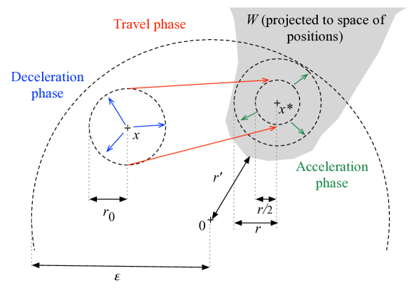
Figure S1: TIllustration of the notation used in the proof of Lemma 3, part (2) (this figure is best viewed in colour). We consider trajectories divided into three phases, namely deceleration (blue), travel (red), and acceleration (green). The ball around the initial point, $x$, is used when bringing the velocity down to a norm bounded by one (deceleration phase). This allows us to use Lemma 3, part (1) in order to bound the probability of travel to a ball centered at $x^{\star}$ of radius $r/2$ (travel phase). Finally, since $W$ may not contain points with velocity bounded by one, the ball centered at $x^{\star}$ of radius $r$ is used to reach velocities contained in $W$ while ensuring position coordinates are also still in $W$.

Appendix E Direct proof of invariance

Let $\mu_{t}$ be the law of $z\left(t\right)$. In the following, we prove invariance by explicitly verifying that the time evolution of the density $\frac{{\rm d}\mu_{t}}{{\rm d}t}=0$ is zero if the initial distribution $\mu_{0}$ is given by $\rho(z)=\pi\left(x\right)\psi\left(v\right)$ in Proposition 1. This is achieved by deriving the forward Kolmogorov equation describing the evolution of the marginal density of the stochastic process. For simplicity, we start by presenting the invariance argument when $\lambda^{\text{{ref}}}=0$.

Notation and description of the algorithm. We denote a pair of position and velocity by $z=\left(x,v\right)\in{\mathbb{R}}^{{\hyperlink{d}{\color[rgb]{0,0,0}{d}}}}\times{\mathbb{R}}^{{\hyperlink{d}{\color[rgb]{0,0,0}{d}}}}$ and we denote translations by $\Phi_{t}(z)=(\Phi_{t}^{\mathrm{pos}}(z),\Phi_{t}^{\mathrm{dir}}(z))=\left(x+vt,v\right)$. The time of the first bounce coincides with the first arrival $T_{1}$ of a PP with intensity $\chi(t)=\mathrm{\lambda}(\Phi_{t}(z))$ where:

$$\mathrm{\lambda}(z)=\max\left\{0,\left\langle\nabla U\left(x\right),v\right\rangle\right\}.$$ (S1)

It follows that the probability of having no bounce in the interval $[0,t]$ is given by:

$$\mathrm{N}\mathrm{o}_{t}(z)=\exp\left(-\int_{0}^{t}\lambda(\Phi_{s}(z)){\rm d}s\right),$$ (S2)

and the density of the random variable $T_{1}$ is given by:

$$q(t_{1};z)= \mathbf{1}[t_{1}>0]\frac{{\rm d}}{{\rm d}t_{1}}\left(1-\mathrm{N}o_{t_{1}}(z)\right)$$ (S3)

$$= \mathbf{1}[t_{1}>0]\mathrm{N}\mathrm{o}_{t_{1}}(z)\mathrm{\lambda}(\Phi_{t_{1}}(z)).$$ (S4)

If a bounce occurs, then the algorithm follows a translation path for time $T_{1}$, at which point the velocity is updated using a bounce operation $C(z)$, defined as:

$$C\left(z\right)=\left(x,R\left(x\right)v\right)$$ (S5)

where

$$R\left(x\right)v=v-2\frac{\left\langle\nabla U\left(x\right),v\right\rangle\nabla U\left(x\right)}{\left\|\nabla U\left(x\right)\right\|^{2}}.$$ (S6)

The algorithm then continues recursively for time $t-T_{1}$, in the following sense: a second bounce time $T_{2}$ is simulated by adding to $T_{1}$ a random increment with density $q(\cdot;C\circ\Phi_{t_{1}}(z))$. If $T_{2}>t$, then the output of the algorithm is $\Phi_{t-t_{1}}\circ C\circ\Phi_{t_{1}}(z)$, otherwise an additional bounce is simulated, etc. More generally, given an initial point $z$ and a sequence $\mathbf{t}=(t_{1},t_{2},\dots)$ of bounce times, the output of the algorithm at time $t$ is given by:

$$\Psi_{\mathbf{t},t}\left(z\right)=\begin{cases}\Phi_{t}(z)&\mathrm{if}\leavevmode\nobreak\ t_{1}>0\leavevmode\nobreak\ \mathrm{or\leavevmode\nobreak\ }\mathbf{t}=(\thinspace),\\ \Psi_{\mathbf{t^{\prime}},t-t_{1}}\left(z\right)\circ C\circ\Phi_{t_{1}}(z)&\mathrm{otherwise,}\end{cases}$$ (S7)

where $(\thinspace)$ denotes the empty list and $\mathbf{t}^{\prime}$ the suffix of $\mathbf{t}$: $\mathbf{t}^{\prime}=(t_{2},t{}_{3},\dots)$. As for the bounce times, they are distributed as follows:

$$T_{1} \sim q(\;\cdot\;;z)$$ (S8)

$$T_{i}-T_{i-1}|T_{1:i-1} \sim q\Big{(}\;\cdot\;;\underbrace{\Psi_{T_{1:i-1},T_{i-1}}(z)}_{\text{Pos. after collision $i-1$}}\Big{)},\;\;\;i\in\{2,3,4,\dots\}$$ (S9)

where $T_{1:i-1}=\left(T_{1},T_{2},\ldots,T_{i-1}\right).$

Decomposition by the number of bounces. Let $h$ denote an arbitrary non-negative measurable test function. We show how to decompose expectations of the form $\mathbb{E}[h(\Psi_{\mathbf{T},t}(z))]$ by the number of bounces in the interval $(0,t)$. To do so, we introduce a function $\#\mathrm{Col}_{t}(\mathbf{t})$, which returns the number of bounces in the interval $(0,t)$:

$$\#\mathrm{Col}_{t}(\mathbf{t})=\min\left\{n\geq 1:t_{n}>t\right\}-1.$$ (S10)

From this, we get the following decomposition:

$$\mathbb{E}[h(\Psi_{\mathbf{T},t}(z))] = \mathbb{E}[h(\Psi_{\mathbf{T},t}(z))\sum_{n=0}^{\infty}\mathbf{1}[\#\mathrm{Col}_{t}(\mathbf{T})=n]]$$ (S11)

$$= \sum_{n=0}^{\infty}\mathbb{E}[h(\Psi_{\mathbf{T},t}(z))\mathbf{1}[\#\mathrm{Col}_{t}(\mathbf{T})=n]].$$ (S12)

On the event that no bounce occurs in the interval $[0,t)$, i.e. $\#\mathrm{Col}_{t}(\mathbf{T})=0$, the function $\Psi_{\mathbf{T},t}(z)$ is equal to $\Phi_{t}(z)$, therefore:

$$\mathbb{E}[h(\Psi_{\mathbf{T},t}(z))\mathbf{1}[\#\mathrm{Col}_{t}(\mathbf{T})=0]] = h(\Phi_{t}(z))\mathbb{P}(\#\mathrm{Col}_{t}(\mathbf{T})=0)$$ (S13)

$$= h(\Phi_{t}(z))\mathrm{N}\mathrm{o}_{t}(z).$$ (S14)

Indeed, on the event that $n\geq 1$ bounces occur, the random variable $h(\Phi_{t}(z))$ only depends on a finite dimensional random vector, $(T_{1},T_{2},\dots,T_{n})$, so we can write the expectation as an integral with respect to the density $\widetilde{q}(t_{1:n};t,z)$ of these variables:

$$\mathbb{E}[h(\Psi_{\mathbf{T},t}(z))\mathbf{1}[\#\mathrm{Col}_{t}(\mathbf{T})=n]]$$ (S15)

$$=\mathbb{E}\left[h(\Psi_{\mathbf{T},t}(z))\mathbf{1}[0<T_{1}<\dots<T_{n}<t<T_{n+1}]\right]$$

$$=\idotsint{}_{0<t_{1}<\dots<t_{n}<t<t_{n+1}}h(\Psi_{t_{1:n},t}(z))q(t_{1};z)\prod_{i=2}^{n+1}q(t-t_{i-1};\Psi_{t_{1:i-1},t_{i-1}}(z)){\rm d}t_{1:n+1}$$

$$=\idotsint{}_{0<t_{1}<\dots<t_{n}<t}h(\Psi_{t_{1:n},t}(z))\widetilde{q}(t_{1:n};t,z){\rm d}t_{1:n},$$ (S16)

where:

$$\widetilde{q}(t_{1:n};t,z)=q(t_{1};z)\times\begin{cases}\mathrm{N}\mathrm{o}_{t-t_{1}}(\Phi_{t_{1}}(z))&\mathrm{if}\leavevmode\nobreak\ n=1\\ \mathrm{N}\mathrm{o}_{t-t_{n}}(\Phi_{t_{1:n},t_{n}}(z))&\prod_{i=2}^{n}q\left(t_{i}-t_{i-1};\Psi_{t_{1:i-1},t_{i-1}}(z)\right)\ \mathrm{if}\leavevmode\nobreak\ n\geq 2.\end{cases}$$

To include Equations (S14) and (S16) under the same notation, we define $t_{1:0}$ to the empty list, $(\thinspace)$, $\widetilde{q}((\thinspace);t,z)=\mathrm{N}\mathrm{o}_{t}(z)$, and abuse the integral notation so that for all $n\in\{0,1,2,\dots\}$:

$$\mathbb{E}[h(\Psi_{\mathbf{T},t}(z))\mathbf{1}[\#\mathrm{Col}_{t}(\mathbf{T})=n]]=\idotsint{}_{0<t_{1}<\dots<t_{n}<t}\thinspace h(\Psi_{t_{1:n},t}(z))\widetilde{q}(t_{1:n};t,z){\rm d}t_{1:n}.$$ (S17)

Marginal density. Let us fix some arbitrary time $t>0$. We seek a convenient expression for the marginal density at time $t$, $\mu_{t}(z)$, given an initial vector $Z\sim\rho$, where $\rho$ is the hypothesized stationary density $\rho(z)=\pi\left(x\right)\psi\left(v\right)$ on $Z$. To do so, we look at the expectation of an arbitrary non-negative measurable test function $h$:

$$\mathbb{E}[h(\Psi_{\mathbf{T},t}(Z))] = \mathbb{E}\Big{[}\mathbb{E}[h(\Psi_{\mathbf{T},t}(Z))|Z]\Big{]}$$ (S18)

$$= \sum_{n=0}^{\infty}\mathbb{E}\Big{[}\mathbb{E}[h(\Psi_{\mathbf{T},t}(Z))\mathbf{1}[\#\mathrm{Col}_{t}(\mathbf{T})=n]|Z]\Big{]}$$ (S19)

$$= \sum_{n=0}^{\infty}\int_{\mathcal{Z}}\rho(z)\idotsint{}_{0<t_{1}<\dots<t_{n}<t}h(\Psi_{t_{1:n},t}(z))\widetilde{q}(t_{1:n};t,z){\rm d}t_{1:n}{\rm d}z$$ (S20)

$$= \sum_{n=0}^{\infty}\;\;\idotsint{}_{0<t_{1}<\dots<t_{n}<t}\int_{\mathcal{Z}}\rho(z)h(\Psi_{t_{1:n},t}(z))\widetilde{q}(t_{1:n};t,z){\rm d}z{\rm d}t_{1:n}$$

$$= \sum_{n=0}^{\infty}\;\;\idotsint{}_{0<t_{1}<\dots<t_{n}<t}\int_{\mathcal{Z}}\rho(\Psi_{t_{1:n},t}^{-1}(z^{\prime}))h(z^{\prime})\widetilde{q}(t_{1:n};t,\Psi_{t_{1:n},t}^{-1}(z^{\prime}))\left|\det D\Psi_{t_{1:n},t}^{-1}\right|{\rm d}z^{\prime}{\rm d}t_{1:n}$$

$$= \int_{\mathcal{Z}}h(z^{\prime})\underbrace{\sum_{n=0}^{\infty}\;\;\idotsint{}_{0<t_{1}<\dots<t_{n}<t}\rho(\Psi_{t_{1:n},t}^{-1}(z^{\prime}))\widetilde{q}(t_{1:n};t,\Psi_{t_{1:n},t}^{-1}(z^{\prime})){\rm d}t_{1:n}}_{\mu_{t}(z^{\prime})}{\rm d}z^{\prime}.$$ (S22)

We used the following in the above derivation successively the law of total expectation, equation (S12), equation (S18), Tonelli’s theorem and the change of variables, $z^{\prime}=\Psi_{t_{1:n},t}(z)$, justified since for any fixed $0<t_{1}<t_{2}<\dots<t_{n}<t<t_{n+1}$, $\Psi_{t_{1:n},t}(\cdot)$ is a bijection (being a composition of bijections). Now the absolute value of the determinant is one since $\Psi_{\mathbf{t},t}\left(z\right)$ is a composition of unit-Jacobian mappings and, by using Tonelli’s theorem again, we obtain that the expression above the brace is necessarily equal to $\mu_{t}(z^{\prime})$ since $h$ is arbitrary.

Derivative. Our goal is to show that for all $z^{\prime}\in\mathcal{Z}$

$$\frac{{\rm d}\mu_{t}(z^{\prime})}{{\rm d}t}=0.$$

Since the process is time homogeneous, once we have computed the derivative, it is enough to show that it is equal to zero at $t=0$. To do so, we decompose the computation according to the terms $I_{n}$ in Equation (S22):

$$\mu_{t}(z^{\prime}) = \sum_{n=0}^{\infty}I_{n}(z^{\prime},t)$$ (S23)

$$I_{n}(z^{\prime},t) = \idotsint{}_{0<t_{1}<\dots<t_{n}<t}\rho(\Psi_{t_{1:n},t}^{-1}(z^{\prime}))\widetilde{q}(t_{1:n};t,\Psi_{t_{1:n},t}^{-1}(z^{\prime})){\rm d}t_{1:n}.$$ (S24)

The categories of terms in Equation (S23) to consider are:

No bounce: $n=0$, $\Psi_{t_{1:n},t}(z)=\Phi_{t}(z)$, or,

Exactly one bounce: $n=1$, $\Psi_{t_{1:n},t}(z)=F_{t,t_{1}}:=\Phi_{t-t_{1}}\circ C\circ\Phi_{t_{1}}(z)$ for some $t_{1}\in(0,t)$, or,

Two or more bounces: $n\geq 2$, $\Psi_{t_{1:n},t}(z)=\Psi_{t-t_{2}}\circ C\circ F_{t_{2},t_{1}}(z)$ for some $0<t_{1}<t_{2}<t$

In the following, we show that the derivative of the terms in the third category, $n\geq 2$, are all equal to zero, while the derivative of the first two categories cancel each other.

No bounce in the interval. From Equation (S14):

$$I_{0}(z^{\prime},t) = \rho(\Phi_{-t}(z^{\prime}))\mathrm{N}\mathrm{o}_{t}(\Phi_{-t}(z^{\prime})).$$ (S25)

We now compute the derivative at zero of the above expression:

$$\left.\frac{{\rm d}}{{\rm d}t}I_{0}(z^{\prime},t)\right|_{t=0} =\mathrm{N}\mathrm{o}_{0} (\Phi_{0}(z^{\prime}))\left.\frac{{\rm d}\rho(\Phi_{-t}(z^{\prime}))}{{\rm d}t}\right|_{t=0}+$$ (S26)

$$\rho(\Phi_{0}(z^{\prime}))\left.\frac{{\rm d}\mathrm{N}\mathrm{o}_{t}(\Phi_{-t}(z^{\prime}))}{{\rm d}t}\right|_{t=0}$$

The first term in the above equation can be simplified as follows:

$$\mathrm{N}\mathrm{o}_{0}(\Phi_{0}(z^{\prime}))\frac{{\rm d}\rho(\Phi_{-t}(z^{\prime}))}{{\rm d}t} = \frac{{\rm d}\rho(\Phi_{-t}(z^{\prime}))}{{\rm d}t}$$ (S28)

$$= \left\langle\frac{\partial\rho(\Phi_{-t}(z^{\prime}))}{\partial\Phi_{-t}^{\mathrm{pos}}(z^{\prime})},\frac{{\rm d}\Phi_{-t}^{\mathrm{pos}}(z^{\prime})}{{\rm d}t}\right\rangle+$$

$$\left\langle\frac{\partial\rho(\Phi_{-t}(z^{\prime}))}{\partial\Phi_{-t}^{\mathrm{dir}}(z^{\prime})},\underbrace{\frac{{\rm d}\Phi_{-t}^{\mathrm{dir}}(z^{\prime})}{{\rm d}t}}_{=\boldsymbol{0}}\right\rangle$$

$$= \left\langle\frac{\partial\rho(z)}{\partial x},-v^{\prime}\right\rangle$$

$$= \left\langle\frac{\partial}{\partial x}\frac{1}{Z}\exp\left(-U(x)\right)\psi\left(v\right),-v^{\prime}\right\rangle$$

$$= \rho(\Phi_{-t}(z^{\prime}))\left\langle\nabla U(x),v^{\prime}\right\rangle,$$ (S30)

where $x=\Phi_{-t}^{\mathrm{pos}}(z^{\prime})$. The second term in Equation (S26) is equal to:

$$\rho(\Phi_{0}(z^{\prime}))\left.\frac{{\rm d}\mathrm{N}\mathrm{o}_{t}(\Phi_{-t}(z^{\prime}))}{{\rm d}t}\right|_{t=0} = -\rho(\Phi_{0}(z^{\prime}))\mathrm{N}\mathrm{o}_{0}(z^{\prime})\lambda(\Phi_{0}(z^{\prime}))$$ (S31)

$$= -\rho(z^{\prime})\lambda(z^{\prime}),$$ (S32)

using Equation (S4). In summary, we have:

$$\left.\frac{{\rm d}}{{\rm d}t}I_{0}(z^{\prime},t)\right|_{t=0}=\rho(z^{\prime})\left\langle\nabla U(x^{\prime}),v^{\prime}\right\rangle-\rho(z^{\prime})\mathrm{\lambda}(z^{\prime}).$$

Exactly one bounce in the interval. From Equation (S16), the trajectory consists in a bounce at a time $T_{1}$, occurring with density (expressed as before as a function of the final point $z^{\prime}$) $q(t_{1};F_{t,t_{1}}^{-1}(z^{\prime}))$, followed by no bounce in the interval $(T_{1},t]$, an event of probability:

$$\mathrm{N}\mathrm{o}_{t-t_{1}}(C\circ\Phi_{t_{1}}(z)) = \mathrm{N}\mathrm{o}_{t-t_{1}}(C\circ\Phi_{t_{1}}\circ F_{t,t_{1}}^{-1}(z^{\prime}))$$ (S33)

$$= \mathrm{N}\mathrm{o}_{t-t_{1}}(\Phi_{t_{1}-t}(z^{\prime})),$$ (S34)

where we used that $C^{-1}=C$. This yields:

$$I_{1}(z^{\prime},t) = \int_{0}^{t}q(t_{1};F_{t,t_{1}}^{-1}(z^{\prime}))\rho(\Psi_{t_{1:1},t}^{-1}(z^{\prime}))\mathrm{N}\mathrm{o}_{t-t_{1}}(\Phi_{t_{1}-t}(z^{\prime})){\rm d}t_{1}.$$ (S35)

To compute the derivative of the above equation at zero, we use again Leibniz’s rule:

$$\left.\frac{{\rm d}}{{\rm d}t}I_{1}(z^{\prime},t)\right|_{t=0}=\rho(C(z^{\prime}))\mathrm{\lambda}(C(z^{\prime})).$$

Two or more bounces in the interval. For a number of bounce, we get:

$$I_{n}(z^{\prime},t)=\int_{0}^{t}\Bigg{[}\;\;\underbrace{\idotsint{}_{t_{2:n}:t_{1}<t_{2}\dots<t_{n}<t}\rho(\Psi_{t_{1:n},t}^{-1}(z^{\prime}))\widetilde{q}(t_{1:n};t,\Psi_{t_{1:n},t}^{-1}(z^{\prime})){\rm d}t_{2:n}}_{\tilde{I}(t_{1},t,z^{\prime})}\Bigg{]}{\rm d}t_{1},$$ (S36)

and hence, using Leibniz’s rule on the integral over $t_{1}$:

$$\left.\frac{{\rm d}}{{\rm d}t}I_{n}(z^{\prime},t)\right|_{t=0}=\tilde{I}(0,0,z^{\prime})=0.$$ (S37)

Putting all terms together. Putting everything together, we obtain:

$$\left.\frac{{\rm d}\mu_{t}(z^{\prime})}{{\rm d}t}\right|_{t=0}=\rho(z^{\prime})\left\langle\nabla U(x^{\prime}),v^{\prime}\right\rangle\underbrace{-\rho(z^{\prime})\lambda(z^{\prime})+\rho(C(z^{\prime}))\lambda(C(z^{\prime})).}$$ (S38)

From the expression of $\mathrm{\lambda}(\cdot)$, we can rewrite the two terms above the brace as follows:

$$-\rho(z^{\prime})\mathrm{\lambda}(z^{\prime})+\rho(C(z^{\prime}))\lambda(C(z^{\prime}))$$

$$= -\rho(z^{\prime})\lambda(z^{\prime})+\rho(z^{\prime})\lambda(C(z^{\prime}))$$

$$= -\rho(z^{\prime})\max\{0,\left\langle\nabla U(x^{\prime}),v^{\prime}\right\rangle\}+\rho(z^{\prime})\max\{0,\left\langle\nabla U(x^{\prime}),R\left(x^{\prime}\right)v^{\prime}\right\rangle\}$$

$$= -\rho(z^{\prime})\max\{0,\left\langle\nabla U(x^{\prime}),v^{\prime}\right\rangle\}+\rho(z^{\prime})\max\{0,\left\langle\nabla U(x^{\prime}),R\left(x^{\prime}\right)v^{\prime}\right\rangle\}$$

$$= -\rho(z^{\prime})\max\{0,\left\langle\nabla U(x^{\prime}),v^{\prime}\right\rangle\}+\rho(z^{\prime})\max\{0,-\left\langle\nabla U(x^{\prime}),v^{\prime}\right\rangle\}$$

$$= -\rho(z^{\prime})\left\langle\nabla U(x^{\prime}),v^{\prime}\right\rangle,$$

where we used that $\rho(z^{\prime})=\rho(C(z^{\prime}))$, $\left\langle\nabla U(x^{\prime}),R\left(x^{\prime}\right)v^{\prime}\right\rangle=-\left\langle\nabla U(x^{\prime}),v^{\prime}\right\rangle$ and $-\max\{0,f\}+\max\{0,-f\}=-f$ for any function $f$. Hence we have $\left.\frac{{\rm d}\mu_{t}(z^{\prime})}{{\rm d}t}\right|_{t=0}=0$, establishing that that the bouncy particle sampler $\lambda^{\text{ref}}=0$ admits $\rho$ as invariant distribution. The invariance for $\lambda^{\text{ref}}>0$ then follows from Lemma 4 given below.

Lemma 4.

Suppose $P_{t}$ is a continuous time Markov kernel and $Q$ is a discrete time Markov kernel which are both invariant with respect to $\mu.$ Suppose we construct for $\lambda^{\text{{ref}}}>0$ a Markov process $\hat{P}_{t}$ as follows: at the jump times of an independent PP with intensity $\lambda^{\text{{ref}}}$ we make a transition with $Q$ and then continue according to $P_{t}$, then $\hat{P}_{t}$ is also $\mu$-invariant.

Proof.

The transition kernel is given by

$$\hat{P}_{t} = e^{-\lambda t}P_{t}+\int_{0}^{t}{\rm d}t_{1}\lambda e^{\lambda t_{1}}e^{-\lambda(t-t_{1})}P_{t-t_{1}}QP_{t_{1}}$$

$$+\int_{0}^{t}{\rm d}t_{1}\int_{t_{1}}^{t_{2}}{\rm d}t_{2}\lambda^{2}e^{\lambda t_{1}}e^{\lambda(t_{2}-t_{1})}e^{-\lambda(t-t_{2})}P_{t-t_{2}}QP_{t_{2}-t_{1}}QP_{t_{1}}+\dots$$

Therefore

$$\mu\hat{P}_{t} = \mu\left(e^{-\lambda t}+\lambda te^{-\lambda t}+\frac{\left(\lambda t\right)^{2}}{2}e^{-\lambda t}\dots\right)$$

$$= \mu.$$

Hence $\hat{P}_{t}$ is $\mu$-invariant. ∎

Appendix F Invariance of the local sampler

The generator of the local BPS is given by

$$\mathcal{L}h(z) = \left\langle\nabla_{x}h\left(x,v\right),v\right\rangle$$

$$+\sum_{f\in F}\lambda_{f}\left(x,v\right)\left\{h(x,R_{f}\left(x\right)v)-h(x,v)\right\}$$

$$+\lambda^{\mathrm{ref}}\int\left(h(x,v^{\prime})-h(x,v)\right)\psi\left(\,\mathrm{d}v^{\prime}\right).$$

The proof of invariance of the local BPS is very similar to the proof of Propostion 1. We have

$$\mathcal{\int L}h(z)\rho\left(z\right){\rm d}z = \int\int\left\langle\nabla_{x}h\left(x,v\right),v\right\rangle\rho\left(z\right){\rm d}z$$ (S42)

$$+\int\int\sum_{f\in F}\lambda_{f}\left(x,v\right)\left\{h(x,R_{f}\left(x\right)v)-h(x,v)\right\}]\rho\left(z\right){\rm d}z$$

$$+\lambda^{\mathrm{ref}}\int\int\int\left(h(x,v^{\prime})-h(x,v)\right)\psi\left(\,\mathrm{d}v^{\prime}\right)\rho\left(z\right){\rm d}z$$

where the term (S42) is straightforwardly equal to 0 while, by integration by parts, the term (S42) satisfies

$$\int\int\left\langle\nabla_{x}h\left(x,v\right),v\right\rangle\rho\left(z\right){\rm d}z=\int\int\left\langle\nabla U\left(x\right),v\right\rangle h\left(x,v\right)\rho\left(z\right){\rm d}z.$$ (S43)

as $h$ is bounded. Now a change-of-variables shows that for any $f\in F$

$$\int\int\lambda_{f}\left(x,v\right)h(x,R_{f}\left(x\right)v)\rho\left(z\right){\rm d}z=\int\int\lambda\left(x,R_{f}\left(x\right)v\right)h(x,v)\rho\left(z\right){\rm d}z$$ (S44)

as $R_{f}^{-1}\left(x\right)v)=R\left(x\right)v$ and $\left\|R_{f}\left(x\right)v\right\|=\left\|v\right\|$ implies $\psi\left(R_{f}\left(x\right)v\right)=\psi\left(v\right)$. So the term (S42) satisfies

$$\int\int\sum_{f\in F}\lambda_{f}\left(x,v\right)\left\{h(x,R_{f}\left(x\right)v)-h(z)\right\}]\rho\left(z\right){\rm d}z$$ (S45)

$$= \int\int\sum_{f\in F}[\lambda\left(x,R_{f}\left(x\right)v\right)-\lambda\left(x,v\right)]h(x,v)\rho\left(z\right){\rm d}z$$

$$= \int\int\sum_{f\in F}[\max\{0,\left\langle\nabla U_{f}(x),R\left(x\right)v\right\rangle\}-\max\{0,\left\langle\nabla U_{f}(x),v\right\rangle\}]h(x,v)\rho\left(z\right){\rm d}z$$

$$= \int\int\sum_{f\in F}[\max\{0,-\left\langle\nabla U_{f}(x),v\right\rangle\}-\max\{0,\left\langle\nabla U_{f}(x),v\right\rangle\}]h(x,v)\rho\left(z\right){\rm d}z$$

$$= -\int\int\sum_{f\in F}[\left\langle\nabla U_{f}\left(x\right),v\right\rangle]h(x,v)\rho\left(z\right){\rm d}z$$

$$= -\int\int\left\langle\nabla U\left(x\right),v\right\rangle]h(x,v)\rho\left(z\right){\rm d}z,$$

where we have used $\left\langle\nabla U_{f}(x),R_{f}\left(x\right)v\right\rangle=-\left\langle\nabla U_{f}(x),v\right\rangle$ and $\max\{0,-f\}-\max\{0,f\}=-f$ for any $f$. Hence, summing (S43)-(S45)-(S42), we obtain$\mathcal{\int L}h(z)\rho\left(z\right){\rm d}z=0$ and the result follows by [7, Proposition 34.7].

Appendix G Calculations in the isotropic normal case

As we do not use refreshment, it follows from the definition of the collision operator that

$$\left\langle x^{(i)},v^{(i)}\right\rangle = \left\langle x^{(i)},v^{(i-1)}-\frac{2\left\langle x^{(i)},v^{(i-1)}\right\rangle}{\left\|x^{(i)}\right\|^{2}}x^{(i)}\right\rangle$$

$$= -\left\langle x^{(i)},v^{(i-1)}\right\rangle=-\left\langle x^{(i-1)},v^{(i-1)}\right\rangle-\tau_{i}$$

$$= \begin{cases}-\sqrt{-\log V_{i}}&\text{if }\left\langle x^{(i-1)},v^{(i-1)}\right\rangle\leq 0\\ -\sqrt{\left\langle x^{(i-1)},v^{(i-1)}\right\rangle^{2}-\log V_{i}}&\text{otherwise}\end{cases},$$

and therefore

$$\left\|x^{(i)}\right\|^{2}=\begin{cases}\left\|x^{(i-1)}\right\|^{2}-\left\langle x^{(i-1)},v^{(i-1)}\right\rangle^{2}-\log V_{i}&\text{ if }\left\langle x^{(i-1)},v^{(i-1)}\right\rangle\leq 0\\ \left\|x^{(i-1)}\right\|^{2}-\log V_{i}&\text{otherwise.}\end{cases}.$$

It follows that $\left\langle x^{(j)},v^{(j)}\right\rangle\leq 0$ for $j>0$ if $\left\langle x^{(0)},v^{(0)}\right\rangle\leq 0$ so, in this case, we have

$$\left\|x^{(i)}\right\|^{2} =\left\|x^{(i-1)}\right\|^{2}-\left\langle x^{(i-1)},v^{(i-1)}\right\rangle^{2}-\log V_{i}$$

$$=\left\|x^{(i-1)}\right\|^{2}+\log V_{i-1}-\log V_{i}$$

$$=\left\|x^{(i-2)}\right\|^{2}-\left\langle x^{(i-1)},v^{(i-1)}\right\rangle^{2}-\log V_{i-1}+\log V_{i-1}-\log V_{i}$$

$$\vdots \vdots$$

$$=\left\|x^{(1)}\right\|^{2}-\left\langle x^{(1)},v^{(1)}\right\rangle^{2}-\log V_{i}$$

In particular for $x^{(0)}=e_{1}$ and $v^{(0)}=e_{2}$ with $e_{i}$ being elements of standard basis of $\mathbb{R}^{d}$, the norm of the position at all points along the trajectory can never be smaller than 1.

Appendix H Supplementary information on the evolutionary parameters inference experiments

H.1 Model

We consider an over-parameterized generalized time reversible rate matrix [29] with $d=10$ corresponding to 4 unnormalized stationary parameters $x_{1},\dots,x_{4}$, and 6 unconstrained substitution parameters $x_{\{i,j\}}$, which are indexed by sets of size 2, i.e. where $i,j\in\left\{1,2,3,4\right\},\thinspace i\neq j$. Off-diagonal entries of $Q$ are obtained via $q_{i,j}=\pi_{j}\exp\left(x_{\{i,j\}}\right)$, where

$$\pi_{j}=\frac{\exp\left(x_{j}\right)}{\sum_{k=1}^{4}\exp\left(x_{k}\right)}.$$

We assign independent standard Gaussian priors on the parameters $x_{i}.$ We assume that a matrix of aligned nucleotides is provided, where rows are species and columns contains nucleotides believed to come from a shared ancestral nucleotide. Given $x=\left(x_{1},\dots,x_{4},x_{\{1,2\}},\dots,x_{\{3,4\}}\right),$ and hence $Q$, the likelihood is a product of conditionally independent continuous time Markov chains over $\{$A, C, G, T$\}$, with “time” replaced by a branching process specified by the phylogenetic tree’s topology and branch lengths. The parameter $x$ is unidentifiable, and while this can be addressed by bounded or curved parameterizations, the over-parameterization provides an interesting challenge for sampling methods, which need to cope with the strong induced correlations.

H.2 Baseline

We compare the BPS against a state-of-the-art HMC sampler [33] that uses Bayesian optimization to adapt the the leap-frog stepsize $\epsilon$ and trajectory length $L$ of HMC. This sampler was shown in [35] to be comparable or better to other state-of-the-art HMC methods such as NUTS. It also has the advantage of having efficient implementations in several languages. We use the author’s Java implementation to compare to our Java implementation of the BPS. Both methods view the objective function as a black box (concretely, a Java interface supporting pointwise evaluation and gradient calculation). In all experiments, we initialize at the mode and use a burn-in of 100 iterations and no thinning. The HMC auto-tuner yielded $\epsilon=0.39$ and $L=100$. For our method, we use the global sampler and the global refreshment scheme.

H.3 Additional experimental results

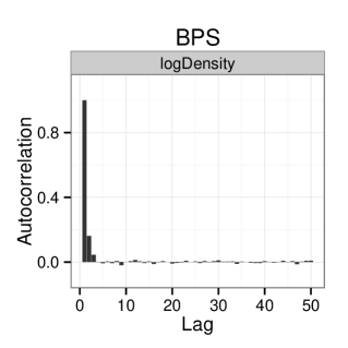
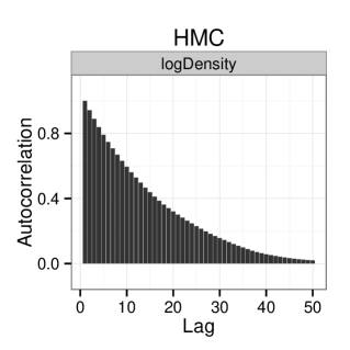
Figure S2: Estimate of the ACF of the log-likelihood statistic for BPS (left) and HMC (right). A similar behavior is observed for the ACF of the other statistics.

To ensure that BPS outperforming HMC does not come from a faulty auto-tuning of HMC parameters, we look at the ESS/s for the log-likelihood statistic when varying the stepsize $\epsilon$. The results in Figure S3(right) show that the value selected by the auto-tuner is indeed reasonable, close to the value 0.02 found by brute force maximization. We repeat the experiments with $\epsilon=0.02$ and obtain the same conclusions. This shows that the problem is genuinely challenging for HMC.

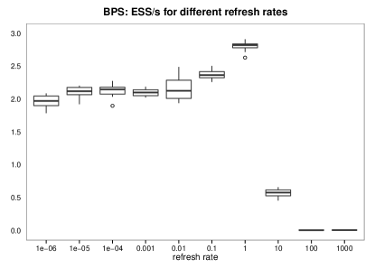
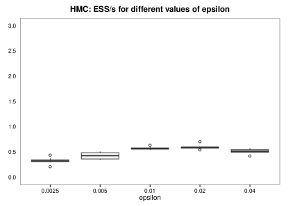
Figure S3: Left: sensitivity of BPS’s ESS/s on the log likelihood statistic. Right: sensitivity of HMC’s ESS/s on the log likelihood statistic. Each setting is replicated 10 times with different algorithmic random seeds.

The BPS algorithm also exhibits sensitivity to $\lambda^{\mathrm{ref}}$. We analyze this dependency in Figure S3(left). We observe an asymmetric dependency, where values higher than 1 result in a significant drop in performance, as they bring the sampler closer to random walk behavior. Values one or more orders of magnitudes lower than 1 have a lower detrimental effect. However for a range of values of $\lambda^{\mathrm{ref}}$ covering six orders of magnitudes, BPS outperforms HMC at its optimal parameters.

References

• [1] R.J. Adler and J.E. Taylor. Topological Complexity of Smooth Random Functions, volume 2019 of Lecture Notes in Mathematics. Springer, Heidelberg, 2011. École d’Été de Probabilités de Saint-Flour XXXIX.
• [2] R. Bardenet, A. Doucet, and C.C. Holmes. Towards scaling up MCMC: An adaptive subsampling approach. In Proceedings of the 31st International Conference on Machine Learning, 2014.
• [3] R. Bardenet, A. Doucet, and C.C. Holmes. On Markov chain Monte Carlo methods for tall data. 2015. Technical report arXiv:1505.02827.
• [4] J. Bierkens, P. Fearnhead, and G. O. Roberts. The zig-zag process and super-efficient Monte Carlo for Bayesian analysis of big data. 2016. Technical report arXiv:1607.03188.
• [5] A. Bouchard-Côté, S.J. Vollmer, and A. Doucet. The bouncy particle sampler: a non-reversible rejection-free Markov chain Monte Carlo method. 2015. Technical report arxiv:1510.02451v1.
• [6] M. Creutz. Global Monte Carlo algorithms for many-fermion systems. Physical Review D, 38(4):1228–1237, 1988.
• [7] M.H.A. Davis. Markov Models & Optimization, volume 49. CRC Press, 1993.
• [8] L. Devroye. Non-uniform Random Variate Generation. Springer-Verlag, New York, 1986.
• [9] M. Einsiedler and T. Ward. Ergodic Theory: with a view towards Number Theory, volume 259 of Graduate Texts in Mathematics. Springer-Verlag, London, 2011.
• [10] J.M. Flegal, J. Hughes, and D. Vats. mcmcse: Monte Carlo Standard Errors for MCMC, 2015. R package version 1.1-2.
• [11] N. Galbraith. On Event-Chain Monte Carlo Methods. Master’s thesis, Department of Statistics, Oxford University, 9 2016.
• [12] J. Geweke. Evaluating the accuracy of sampling-based approaches to the calculation of posterior moments. Bayesian Statistics, 4:169–193, 1992.
• [13] M. Girolami and B. Calderhead. Riemann manifold Langevin and Hamiltonian Monte Carlo methods. Journal of the Royal Statistical Society: Series B (Statistical Methodology), 73(2):123–214, 2011.
• [14] M. Hairer. Convergence of Markov processes. http://www.hairer.org/notes/Convergence.pdf, 2010. Lecture notes, University of Warwick.
• [15] K. Hayasaka, Takashi G., and Satoshi H. Molecular phylogeny and evolution of primate mitochondrial DNA. Molecular Biology and Evolution, 5:626–644, 1988.
• [16] M.D. Hoffman and A. Gelman. The no-U-turn sampler: Adaptively setting path lengths in Hamiltonian Monte Carlo. Journal of Machine Learning Research, 15(4):1593–1623, 2014.
• [17] A.M. Horowitz. A generalized guided Monte Carlo algorithm. Physics Letters B, 268(2):247–252, 1991.
• [18] J.P. Huelsenbeck and F. Ronquist. MRBAYES: Bayesian inference of phylogenetic trees. Bioinformatics, 17(8):754–755, 2001.
• [19] T.A. Kampmann, H.H. Boltz, and J. Kierfeld. Monte Carlo simulation of dense polymer melts using event chain algorithms. Journal of Chemical Physics, (143):044105, 2015.
• [20] J. S. Liu. Monte Carlo Strategies in Scientific Computing. Springer, 2008.
• [21] D. Maclaurin and R.P. Adams. Firefly Monte Carlo: Exact MCMC with subsets of data. In Uncertainty in Artificial Intelligence, volume 30, pages 543–552, 2014.
• [22] M. Michel, S.C. Kapfer, and W. Krauth. Generalized event-chain Monte Carlo: Constructing rejection-free global-balance algorithms from infinitesimal steps. Journal of Chemical Physics, 140(5):054116, 2014.
• [23] M. Michel, J. Mayer, and W. Krauth. Event-chain Monte Carlo for classical continuous spin models. Europhysics Letters, (112):20003, 2015.
• [24] R.M. Neal. Markov chain Monte Carlo using Hamiltonian dynamics. In Handbook of Markov Chain Monte Carlo. Chapman & Hall/CRC, 2011.
• [25] Y. Nishikawa, M. Michel, W. Krauth, and K. Hukushima. Event-chain Monte Carlo algorithm for the Heisenberg model. Physical Review E, (92):063306, 2015.
• [26] M. Ottobre. Markov chain Monte Carlo and irreversibility. Reports on Mathematical Physics, 77:267–292, 2016.
• [27] E.A. J. F. Peters and G. de With. Rejection-free Monte Carlo sampling for general potentials. Physical Review E, 85:026703, 2012.
• [28] G. O. Roberts and J.S. Rosenthal. Optimal scaling for various Metropolis-Hastings algorithms. Statistical Science, 16(4):351–367, 2001.
• [29] S. Tavaré. Some probabilistic and statistical problems in the analysis of DNA sequences. Lectures on Mathematics in the Life Sciences, 17:56–86, 1986.
• [30] Y. W. Teh, A. H. Thiéry, and S. J. Vollmer. Consistency and fluctuations for stochastic gradient Langevin dynamics. Journal of Machine Learning Research, 17:1–33, 2016.
• [31] V.H. Thanh and C. Priami. Simulation of biochemical reactions with time-dependent rates by the rejection-based algorithm. Journal of Chemical Physics, 143(5):054104, 2015.
• [32] M.J. Wainwright and M.I. Jordan. Graphical models, exponential families, and variational inference. Foundations and Trends in Machine Learning, 1(1-2):1–305, 2008.
• [33] Z. Wang, S. Mohamed, and N. de Freitas. Adaptive Hamiltonian and Riemann manifold Monte Carlo. In Proceedings of the 30th International Conference on Machine Learning, pages 1462–1470, 2013.
• [34] M. Welling and Y. W. Teh. Bayesian learning via stochastic gradient Langevin dynamics. In Proceedings of the 28th International Conference on Machine Learning, pages 681–688, 2011.
• [35] T Zhao, Z. Wang, A. Cumberworth, J. Gsponer, N. de Freitas, and A. Bouchard-Côté. Bayesian analysis of continuous time Markov chains with application to phylogenetic modelling. Bayesian Analysis, 11:1203–1237, 2016.