Elasto-capillarity Simulations based on the Navier–Stokes–Cahn–Hilliard Equations

Abstract

We consider a computational model for complex-fluid-solid interaction based on a diffuse-interface model for the complex fluid and a hyperelastic-material model for the solid. The diffuse-interface complex-fluid model is described by the incompressible Navier–Stokes–Cahn–Hilliard equations with preferential-wetting boundary conditions at the fluid-solid interface. The corresponding fluid traction on the interface includes a capillary-stress contribution, and the dynamic interface condition comprises the traction exerted by the non-uniform fluid-solid surface tension. We present a weak formulation of the aggregated complex-fluid-solid-interaction problem, based on an Arbitrary-Lagrangian-Eulerian formulation of the Navier–Stokes–Cahn–Hilliard equations and a proper reformulation of the complex-fluid traction and the fluid-solid surface tension. To validate the presented complex-fluid-solid-interaction model, we present numerical results and conduct a comparison to experimental data for a droplet on a soft substrate.

0.1 Introduction

Complex fluids are fluids that consist of multiple constituents, e.g. of multiple phases of the same fluid (gas, liquid or solid) or of multiple distinct species (e.g. water and air). The interaction of such complex fluids with elastic solids leads to multitudinous intricate physical phenomena. Examples are durotaxis, viz., seemingly spontaneous migration of liquid droplets on solid substrates with an elasticity gradient [19], or capillary origami, viz., large-scale solid deformations induced by capillary forces [17]. Complex-Fluid-Solid Interaction (CFSI) is moreover of fundamental technological importance in a wide variety of applications, such as inkjet printing and additive manufacturing.

Despite significant progress in models and computational techniques for the interaction of solids and classical fluids (see [4, 20] for an overview), and for complex fluids separately (see, e.g., [15, 13, 12, 1, 11, 2]), complex-fluid-solid interaction has remained essentially unexplored. A notable exception is the computational CFSI model based on the Navier–Stokes–Korteweg equations in [6].

In this contribution we consider a computational model for complex-fluid-solid interaction based on a diffuse-interface complex-fluid model and a hyperelastic solid model with a Saint Venant–Kirchhoff stored-energy functional. The diffuse-interface complex-fluid model is described by the incompressible Navier–Stokes–Cahn–Hilliard (NSCH) equations. The interaction of the complex fluid with the solid substrate is represented by dynamic and kinematic interface conditions and a preferential-wetting boundary condition. The traction exerted by the complex fluid on the fluid-solid interface comprises a non-standard capillary-stress contribution, in addition to the standard pressure and viscous-stress components. The dynamic condition imposes equilibrium of this complex-fluid traction, the traction exerted by the hyperelastic solid and the traction due to the non-uniform fluid-solid surface tension. We present a weak formulation of the aggregated complex-fluid-solid-interaction problem, based on an Arbitrary-Lagrangian-Eulerian (ALE) formulation of the NSCH system and a suitable weak representation of the complex-fluid traction and the non-uniform fluid-solid surface tension.

To evaluate the capability of the considered complex-fluid-solid-interaction model to describe elasto-capillary phenomena, we consider numerical experiments for a test case pertaining to a droplet on a soft substrate, and we present a comparison to experimental data from [18].

The remainder of this contribution is organized as follows. Section 0.2 presents a specification and discussion of the considered complex-fluid-solid-interaction problem. In Section 0.3 we treat the weak formulation of the aggregated fluid-solid-interaction problem. Section 0.4 is concerned with numerical experiments and results. Concluding remarks are presented in Section 0.5.

0.2 Problem Statement

To accommodate the complex-fluid-solid system, we consider a time interval $(0,T)\subseteq\mathbb{R}_{>0}$ and two simply-connected time-dependent open subsets $\smash[tb]{\smash[tb]{\Omega^{\mathrm{f}}_{t}}}\subset\mathbb{R}^{d}$ ($d=2,3$) and $\smash[tb]{\smash[tb]{\Omega^{\mathrm{s}}_{t}}}\subset\mathbb{R}^{d}$, which hold the complex-fluid and solid, respectively. The fluid-solid interface corresponds to $\smash[tb]{\Gamma_{t}:=\partial\smash[tb]{\Omega^{\mathrm{f}}_{t}}\cap\partial\smash[tb]{\Omega^{\mathrm{s}}_{t}}}\neq\emptyset$. We assume that the time-dependent configuration $\smash[tb]{\Omega_{t}:=\mathrm{int}(\mathrm{cl}\,\smash[tb]{\Omega^{\mathrm{f}}_{t}}\cup\mathrm{cl}\,\smash[tb]{\Omega^{\mathrm{s}}_{t}})}$ is the image of a time-dependent transformation $\hat{\chi}$ acting on a fixed reference domain $\smash[tb]{\hat{\Omega}:=\mathrm{int}(\mathrm{cl}\,\smash[tb]{\hat{\Omega}{}^{\mathrm{f}}}\cup\mathrm{cl}\,\smash[tb]{\hat{\Omega}{}^{\mathrm{s}}})}$ such that $\smash[tb]{\Omega^{\mathrm{f}}_{t}}=\hat{\chi}\smash[tb]{\hat{\Omega}{}^{\mathrm{f}}}$ and $\smash[tb]{\Omega^{\mathrm{s}}_{t}}=\hat{\chi}\smash[tb]{\hat{\Omega}{}^{\mathrm{s}}}$. The restrictions of ${\hat{\chi}}$ to $\smash[tb]{\hat{\Omega}{}^{\mathrm{f}}}$ and $\smash[tb]{\hat{\Omega}{}^{\mathrm{s}}}$ are denoted by ${\hat{\chi}}^{\mathrm{f}}$ and ${\hat{\chi}}^{\mathrm{s}}$, respectively. The reference domains $\smash[tb]{\hat{\Omega}{}^{\mathrm{f}}}:=\smash[tb]{\Omega^{\mathrm{f}}_{0}}$ and $\smash[tb]{\hat{\Omega}{}^{\mathrm{s}}}:=\smash[tb]{\Omega^{\mathrm{s}}_{0}}$ are identified with the initial configurations.

0.2.1 Navier–Stokes–Cahn–Hilliard Complex-Fluid Model

We consider a complex fluid composed of two immiscible incompressible constituents, separated by a thin diffuse interface. The behavior of the complex fluid is described by the Navier–Stokes–Cahn–Hilliard (NSCH) equations. The two species are identified by an order parameter $\varphi:\smash[tb]{\Omega^{\mathrm{f}}_{t}}\to[-1,1]$. Typically, $\varphi$ is selected as either volume fraction [12, 1, 13] or mass fraction [15, 11], such that $\varphi=1$ (resp. $\varphi=-1$) pertains to a pure species-1 (resp. species-2) composition of the fluid, and $\varphi\in(-1,1)$ indicates a mixture. Depending on the definition of the phase indicator $\varphi$ as mass or volume fraction, and the definition of mixture velocity as mass-averaged or volume-averaged species velocity, various forms of the NSCH equations can be derived. In mass-averaged-velocity formulations, the mixture is generally quasi-incompressible. In volume-averaged-velocity formulations, the mixture is incompressible. We select $\varphi$ as volume fraction and consider a volume-averaged-velocity formulation. The behavior of the complex fluid is described by [2, 13]:

$$\left.\begin{aligned} \partial_{t}(\rho{u})+\nabla\cdot{}(\rho{}u\otimes{}u)+\nabla{}p-\nabla\cdot{}\tau+\tilde{\sigma}\epsilon\nabla\cdot{}(\nabla\varphi\otimes\nabla\varphi)&=0\\ \nabla\cdot{}{}u&=0\\ \partial_{t}{\varphi}+\nabla\cdot{}(\varphi{}u)-\gamma\Delta\mu&=0\\ \mu+\tilde{\sigma}\epsilon\Delta\varphi-\tilde{\sigma}\epsilon^{-1}W^{\prime}(\varphi)&=0\end{aligned}\right\}\text{ in }\smash[tb]{\Omega^{\mathrm{f}}_{t}}$$ (1)

with $\rho:=\rho(\varphi)=\rho_{1}(1+\varphi)/2+\rho_{2}(1-\varphi)/2$ as mixture density, $u:\smash[tb]{\Omega^{\mathrm{f}}_{t}}\to\mathbb{R}^{d}$ as volume-averaged mixture velocity, $p=p:\smash[tb]{\Omega^{\mathrm{f}}_{t}}\to\mathbb{R}$ as pressure, $\tau=\nu\nabla^{s}u$ as viscous-stress tensor and $\mu:\smash[tb]{\Omega^{\mathrm{f}}_{t}}\to\mathbb{R}$ as chemical potential. The mixture viscosity is defined as $\nu:=\nu(\varphi)=\nu_{1}(1+\varphi)/2+\nu_{2}(1-\varphi)/2$. The parameter $\tilde{\sigma}$ is related to the fluid-fluid surface tension $\sigma$ by $2\sqrt{2}\,\tilde{\sigma}=3\,\sigma$, and $\gamma>0$ designates mobility. The energy density associated with mixing of the constituents is represented by the standard double-well potential $W(\varphi)=\frac{1}{4}(\varphi^{2}-1)^{2}$. The parameter $\epsilon>0$ controls the thickness of the diffuse interface between the fluid constituents.

Suitable initial conditions for (1) are provided by a specification of the initial phase distribution and the initial velocity, according to $\varphi(0,\cdot)=\varphi_{0}$ and $u(0,\cdot)=u_{0}$, with $\varphi_{0}:\smash[tb]{\Omega^{\mathrm{f}}_{0}}\to[-1,1]$ and $u_{0}:\smash[tb]{\Omega^{\mathrm{f}}_{0}}\to\mathbb{R}^{d}$ exogenous data. Equations (1₁), (1₃) and (1₄) are typically furnished with Dirichlet or Neumann boundary conditions:

$$\begin{aligned} u&=g{}^{u}_{\mathrm{D}}&&\text{on }\Gamma^{u}_{\mathrm{D}}\\ \varphi&=g^{\varphi}_{\mathrm{D}}&&\text{on }\Gamma^{\varphi}_{\mathrm{D}}\\ \mu&=g{}^{\mu}_{\mathrm{D}}&&\text{on }\Gamma^{\mu}_{\mathrm{D}}\end{aligned}\qquad\qquad\begin{aligned} -pn+\tau{}n-\tilde{\sigma}\epsilon\partial_{n}\varphi\nabla\varphi&=g{}^{u}_{\mathrm{N}}&&\text{on }\Gamma^{u}_{\mathrm{N}}\\ -\tilde{\sigma}\epsilon\partial_{n}\phi&=g{}^{\varphi}_{\mathrm{N}}&&\text{on }\Gamma^{\varphi}_{\mathrm{N}}\\ \gamma\partial_{n}\mu&=g{}^{\mu}_{\mathrm{N}}&&\text{on }\Gamma^{\mu}_{\mathrm{N}}\end{aligned}$$ (2)

with $n$ the exterior unit normal vector to $\partial\smash[tb]{\Omega^{\mathrm{f}}_{t}}$. The right-hand sides in (2) correspond to exogenous data. It generally holds that $\smash[tb]{\Gamma_{\mathrm{D}}^{(\cdot)}\cap\Gamma_{\mathrm{N}}^{(\cdot)}}=\emptyset$. The Neumann condition in (2₁) provides a specification of the fluid traction on the boundary $\smash[tb]{\Gamma_{\mathrm{N}}^{u}}$. If $\smash[tb]{\Gamma_{\mathrm{N}}^{\mu}}$ corresponds to a material boundary, homogeneous data $\smash[tb]{g_{\mathrm{N}}^{\mu}}=0$ provide phase conservation at the boundary. Indeed, from (1₃), the Neumann condition in (2₃) and the Reynolds transport theorem it follows that:

$$\frac{d}{dt}\int_{\smash[tb]{\Omega^{\mathrm{f}}_{t}}}\varphi=\int_{\partial\smash[tb]{\Omega^{\mathrm{f}}_{t}}\setminus\Gamma_{\mathrm{N}}^{\mu}}\big{(}\gamma\partial_{n}\mu-\varphi(u_{n}-w_{n})\big{)}-\int_{\Gamma_{\mathrm{N}}^{\mu}}\varphi(u_{n}-w_{n})+\int_{\Gamma_{\mathrm{N}}^{\mu}}g_{\mathrm{N}}^{\mu}$$ (3)

with $u_{n}$ and $w_{n}$ the normal velocities of the fluid and of the boundary, respectively. Material boundaries satisfy $u_{n}=w_{n}$ and, accordingly, the penultimate term in (3) vanishes. Therefore, the contribution of $\smash[tb]{\Gamma_{\mathrm{N}}^{\mu}}$ to production of $\varphi$ vanishes if $\smash[tb]{g{}_{\mathrm{N}}^{\mu}}=0$. An important alternative to (2₂), is the nonlinear Robin-type condition

$$\tilde{\sigma}\epsilon\partial_{n}\varphi+\sigma_{\mathrm{W}}^{\prime}(\varphi)=0\quad\text{on }\Gamma_{\mathrm{W}}$$ (4)

with $\sigma_{\mathrm{W}}(\varphi)=\tfrac{1}{4}(\varphi^{3}-3\varphi)(\sigma_{2}-\sigma_{1})+\tfrac{1}{2}(\sigma_{1}+\sigma_{2})$ the surface tension of the complex-fluid-solid interface, and $\sigma_{1}>0$ and $\sigma_{2}>0$ the fluid-solid surface tensions of species 1 and 2, respectively; see [14]. Note that $\sigma_{\mathrm{W}}(\cdot)$ provides an interpolation of the pure-species fluid-solid surface tensions, i.e. $\sigma_{\mathrm{W}}(1)=\sigma_{1}$ and $\sigma_{\mathrm{W}}(-1)=\sigma_{2}$. Equation (4) describes preferential wetting of $\smash[tb]{\Gamma_{\mathrm{W}}}$ by the two fluid components. In particular, the angle $\theta_{\mathrm{s}}=\arccos((\sigma_{2}-\sigma_{1})/\sigma)$ corresponds to the static contact angle between the diffuse interface and $\Gamma_{\mathrm{W}}$ (interior to fluid 1). Interaction of the complex fluid (1) with a solid substrate is modeled by Dirichlet condition (2₁), (homogeneous) Neumann condition (2₃), and preferential-wetting condition (4).

0.2.2 Hyperelastic Saint Venant–Kirchhoff Solid Model

We consider a hyperelastic solid with Saint Venant–Kirchhoff stress-strain relation. Denoting the initial density of the solid by $\hat{\rho}:=\rho_{0}:\smash[tb]{\hat{\Omega}{}^{\mathrm{s}}}\to\mathbb{R}_{>0}$, the solid deformation $\hat{\chi}^{\mathrm{s}}:\smash[tb]{\hat{\Omega}{}^{\mathrm{s}}}\to\smash[tb]{\Omega^{\mathrm{s}}_{t}}$ satisfies the equation of motion:

$$\hat{\rho}\partial_{t}^{2}\hat{\chi}^{\mathrm{s}}-\hat{\nabla}\cdot{}\hat{P}=0\quad\text{ in }\smash[tb]{\hat{\Omega}{}^{\mathrm{s}}}$$ (5)

with $\hat{P}$ the first Piola–Kirchhoff stress tensor and $\hat{\nabla}\cdot$ the divergence operator in the reference configuration. For hyperelastic materials, $\hat{\nabla}\cdot\hat{P}$ is the vector-valued function such that $-\int_{\smash[tb]{\hat{\Omega}{}^{\mathrm{s}}}}\hat{x}\cdot(\hat{\nabla}\cdot{}\hat{P})=\mathcal{W}^{\prime}(\hat{\chi}^{\mathrm{s}};\hat{x})$ for all $\hat{x}\in{}C^{\infty}_{0}(\smash[tb]{\hat{\Omega}{}^{\mathrm{s}}},\mathbb{R}^{d})$, with $\mathcal{W}$ the stored-energy functional, $\mathcal{W}^{\prime}(\hat{\chi}^{\mathrm{s}};\cdot)$ its Fréchet derivative at $\hat{\chi}^{\mathrm{s}}$, and $\smash[tb]{C^{\infty}_{0}(\smash[tb]{\hat{\Omega}{}^{\mathrm{s}}},\mathbb{R}^{d})}$ the class of $\mathbb{R}^{d}$-valued smooth functions with compact support in $\smash[tb]{\hat{\Omega}{}^{\mathrm{s}}}$. Denoting by $F:=F(\hat{\chi}^{\mathrm{s}})$ the deformation tensor and by $E:=\tfrac{1}{2}(F^{T}F-I)$ the Green–Lagrange strain tensor, the Saint Venant–Kirchhoff relation specifies the strain-energy density associated with $\hat{\chi}^{\mathrm{s}}$ as $\tfrac{1}{2}\lambda_{\mathrm{L}}(\mathrm{tr}\,E)^{2}+\mu_{\mathrm{L}}(\mathrm{tr}\,E^{2})$ with $\lambda_{\mathrm{L}}$ and $\mu_{\mathrm{L}}$ the Lamé parameters.

The identification of the reference configuration and the initial configuration yields the initial condition $\hat{\chi}^{\mathrm{s}}_{0}=\mathrm{Id}$. Equation (5) is generally furnished with Dirichlet or Neumann conditions:

$$\hat{\chi}^{\mathrm{s}}=g^{\hat{\chi}}_{\mathrm{D}}\quad\text{on }\hat{\Gamma}_{\mathrm{D}}^{\hat{\chi}}\qquad\hat{P}\hat{n}=g^{\hat{\chi}}_{\mathrm{N}}\quad\text{on }\hat{\Gamma}_{\mathrm{N}}^{\hat{\chi}}$$ (6)

with $\smash[tb]{g^{\hat{\chi}}_{\mathrm{D}}}$ and $\smash[tb]{g^{\hat{\chi}}_{\mathrm{N}}}$ deformation and traction data on $\smash[tb]{\hat{\Gamma}_{\mathrm{D}}^{\hat{\chi}}}$ and $\smash[tb]{\hat{\Gamma}_{\mathrm{N}}^{\hat{\chi}}}$, respectively.

0.2.3 Interface Conditions

The complex fluid (1) and solid (5) are interconnected at the interface by kinematic and dynamic interface conditions. The kinematic condition identifies the mixture velocity and the structural velocity at the interface. This condition can be interpreted as a Dirichlet boundary condition for fluid velocity in accordance with (2₁):

$$\qquad{}u=g^{u}_{\mathrm{D}}:=\partial_{t}\hat{\chi}^{\mathrm{s}}\circ{}\hat{\chi}^{-1}\text{ on }\Gamma_{t}\subseteq\Gamma_{\mathrm{D}}^{u}$$ (7)

Kinematic condition (7) constitutes a partial solid-wall condition for (1). The condition is complemented by a homogeneous Neumann condition (2₃) to impose conservation of phase, and wettability boundary condition (4).

The dynamic condition imposes equilibrium of the fluid and solid tractions and the traction exerted on the interface by the fluid-solid surface tension. The traction due to the fluid-solid surface tension is given by the Young-Laplace relation for non-uniform surface tension according to $\Sigma^{\mathrm{fs}}=\sigma_{\mathrm{W}}(\varphi)\kappa{}\,n+\nabla_{\Gamma}\sigma_{\mathrm{W}}(\varphi)$, with $\kappa$ as the additive curvature of $\Gamma_{t}$ and $\nabla_{\Gamma}(\cdot)$ the tangential gradient on $\Gamma_{t}$; see, e.g., [10]. We adopt the convention that curvature is negative if the osculating circle in the normal plane is located in the fluid domain. The complex fluid in (1) exerts traction $\smash[tb]{\Sigma{}^{\mathrm{f}}}:=pn-\tau{}n+\tilde{\sigma}\epsilon\partial_{n}\varphi\nabla\varphi$ on the interface; cf. (2₁). Note the capillary-stress contribution, $\tilde{\sigma}\epsilon\partial_{n}\varphi\nabla\varphi$, to the fluid traction. The traction exerted by the solid (5) is $\smash[tb]{\hat{\Sigma}{}^{\mathrm{s}}}:=-\hat{P}\hat{n}$ with $\hat{n}$ the exterior unit normal vector to $\partial\smash[tb]{\hat{\Omega}{}^{\mathrm{s}}}$; cf. (6). To account for the fact that fluid traction and surface-tension traction are expressed in the current configuration and solid traction is expressed in the reference configuration, we consider the dynamic condition in distributional form:

$$\int_{\hat{\Gamma}}\hat{v}\cdot{}\hat{\Sigma}{}^{\mathrm{s}}\,\mathrm{d}{}\hat{s}=-\int_{\Gamma_{t}}\big{(}\hat{v}\circ{}\hat{\chi}^{-1}\big{)}\cdot\big{(}\Sigma{}^{\mathrm{f}}+\Sigma{}^{\mathrm{fs}}\big{)}\,\mathrm{d}{}s\quad\forall{}\hat{v}\in{}C^{\infty}_{0}(\hat{\Gamma})$$ (8)

with $\mathrm{d}\hat{s}$ and $\mathrm{d}{}s$ the surface measures carried by $\hat{\Gamma}$ and $\Gamma_{t}$, respectively. A precise interpretation of (8) based on weak traction evaluation is presented in Section 0.3.2.

0.3 Weak Formulation

In this section we present a consistent weak formulation of the fluid-solid-interaction problem in Section 0.2. We first consider a weak Arbitrary-Lagrangian-Eulerian (ALE) formulation of the NSCH system (1) in Section 0.3.1. Section 0.3.2 presents a weak formulation of aggregated FSI problem, including a weak formulation of the solid subsystem (5) and an appropriate weak formulation of the traction exerted by the fluid on the solid at the interface in conformity with the dynamic condition.

0.3.1 ALE Formulation of NSCH Equations

To accommodate the motion of the fluid domain, we consider a weak formulation of (1) in ALE form. The weak formulation is set in the current configuration. The deformation of the fluid domain, $\hat{\chi}^{\mathrm{f}}$, induces domain velocity $\hat{w}:=\partial_{t}\hat{\chi}^{\mathrm{f}}$. To derive the ALE formulation, we note that

$$\int_{\smash[tb]{\Omega^{\mathrm{f}}_{t}}}z\partial_{t}{}\psi=\frac{d}{dt}\int_{\smash[tb]{\Omega^{\mathrm{f}}_{t}}}z\psi-\int_{\smash[tb]{\Omega^{\mathrm{f}}_{t}}}\nabla\cdot{}{}\big{(}\psi{}w{}z)-\int_{\smash[tb]{\Omega^{\mathrm{f}}_{t}}}\psi\partial_{t}z=\frac{d}{dt}\int_{\smash[tb]{\Omega^{\mathrm{f}}_{t}}}z\psi-\int_{\smash[tb]{\Omega^{\mathrm{f}}_{t}}}z\nabla\cdot{}(\psi{}w)$$ (9)

for all $\smash[tb]{\hat{z}\in{}C^{\infty}(\smash[tb]{\hat{\Omega}{}^{\mathrm{f}}})}$ and $\smash[tb]{\psi\in{}C^{\infty}(\smash[tb]{\Omega^{\mathrm{f}}_{t}})}$, with $z=\hat{z}\circ{}\hat{\chi}^{-1}$ and $w=\hat{w}\circ{}\hat{\chi}^{-1}$. The identities in (9) follow from the transport theorem and $\partial_{t}(\hat{z}\circ{}\hat{\chi}^{-1})=-w\cdot\nabla{}z$. From (9) it follows that (1₁) and (1₃) subject to (2) can be recast into the weak ALE form:

$$d_{t}\langle\rho{}u,v\rangle+\mathcal{A}_{\mathrm{N}}(u,w,\varphi;v)+\mathcal{B}(p,v) =\mathcal{L}_{\mathrm{N}}(u,w,\varphi,p;v) \forall\hat{v}\in{C}^{\infty}(\smash[tb]{\hat{\Omega}{}^{\mathrm{f}}},\mathbb{R}^{d})$$ (10)

$$d_{t}\langle\varphi,z\rangle+\mathcal{A}_{\mathrm{C}}(u,w,\varphi,\mu;z) =\mathcal{L}_{\mathrm{C}}(u,w,\varphi,\mu;z) \forall{}\hat{z}\in{C}^{\infty}(\smash[tb]{\hat{\Omega}{}^{\mathrm{f}}})$$

with $\langle{}\rho{}u,v\rangle=\int_{\smash[tb]{\Omega^{\mathrm{f}}_{t}}}v\cdot\rho{}u$ and $\langle\varphi,z\rangle=\int_{\smash[tb]{\Omega^{\mathrm{f}}_{t}}}z\,\varphi$, and

$$\mathcal{A}_{\mathrm{N}}(u,w,\varphi;v) =\int_{\smash[tb]{\Omega^{\mathrm{f}}_{t}}}\nabla{}v:\big{(}\tau-\rho{}u\otimes(u-w)-\tilde{\sigma}\epsilon\nabla\varphi\otimes\nabla\varphi\big{)}$$

$$\mathcal{L}{}_{\mathrm{N}}(u,w,\varphi,p;v) =\int_{\Gamma_{\mathrm{N}}^{u}}v\cdot{}g_{\mathrm{N}}^{u}-\int_{\partial\smash[tb]{\Omega^{\mathrm{f}}_{t}}\setminus\Gamma_{\mathrm{N}}^{u}}v\cdot{}\Sigma^{\mathrm{f}}-\int_{\partial\smash[tb]{\Omega^{\mathrm{f}}_{t}}}v\cdot\rho{}u(u_{n}-w_{n})$$

$$\mathcal{A}_{\mathrm{C}}(u,w,\varphi,\mu;z) =\int_{\smash[tb]{\Omega^{\mathrm{f}}_{t}}}\nabla{}z\cdot\big{(}\gamma\nabla\mu-\varphi(u-w)\big{)}$$ (11)

$$\mathcal{L}_{\mathrm{C}}(u,w,\varphi,\mu;z) =\int_{\Gamma_{\mathrm{N}}^{\mu}}z\,g_{\mathrm{N}}^{\mu}+\int_{\partial\smash[tb]{\Omega^{\mathrm{f}}_{t}}\setminus\Gamma_{\mathrm{N}}^{\mu}}z\,\gamma\partial_{n}\mu-\int_{\partial\smash[tb]{\Omega^{\mathrm{f}}_{t}}}z\,\varphi(u_{n}-w_{n})$$

$$\mathcal{B}(p,v) =\int_{\smash[tb]{\Omega^{\mathrm{f}}_{t}}}-p\,\nabla\cdot{}{}v$$

From (1₂) and (1₄), the Neumann condition in (2₂) and the wetting condition (4), we moreover infer:

$$\mathcal{B}(q,u) =0 \forall{}q\in{C}^{\infty}(\smash[tb]{\Omega^{\mathrm{f}}_{t}})$$ (12)

$$\mathcal{A}_{\mathrm{P}}(\varphi;\mu,y) =\mathcal{L}_{\mathrm{P}}(\varphi,y) \forall{}y\in{C}^{\infty}(\smash[tb]{\Omega^{\mathrm{f}}_{t}})$$

with

$$\mathcal{A}_{\mathrm{P}}(\varphi;\mu,y) =\int_{\smash[tb]{\Omega^{\mathrm{f}}_{t}}}y\big{(}\mu-\tilde{\sigma}\epsilon^{-1}W^{\prime}(\varphi)\big{)}-\int_{\smash[tb]{\Omega^{\mathrm{f}}_{t}}}\nabla{}y\cdot\tilde{\sigma}\epsilon\nabla\varphi-\int_{\Gamma_{\mathrm{W}}}y{}f^{\prime}(\varphi)$$ (13)

$$\mathcal{L}_{\mathrm{P}}(\varphi,y) =\int_{\Gamma_{\mathrm{N}}^{\varphi}}y\,g^{\varphi}_{\mathrm{N}}-\int_{\partial\smash[tb]{\Omega^{\mathrm{f}}_{t}}\setminus(\Gamma_{\mathrm{W}}\cup\Gamma_{\mathrm{N}}^{\varphi})}y\,\tilde{\sigma}\epsilon\partial_{n}\varphi$$

It is important to note that the fluid-solid interface satisfies $\Gamma_{t}\subseteq\Gamma_{\mathrm{W}}\cap\Gamma_{\mathrm{N}}^{\mu}\cap\Gamma_{\mathrm{D}}^{u}$.

The configuration of the fluid domain, $\hat{\chi}^{\mathrm{f}}$, can be constructed in various manners. We select $\hat{\chi}^{\mathrm{f}}=h_{\hat{\chi}^{\mathrm{s}}|_{\hat{\Gamma}}}$ as the harmonic extension of the trace of the solid displacement on the interface onto $\smash[tb]{\hat{\Omega}{}^{\mathrm{f}}}$. Accordingly, it holds that $\hat{w}=\partial_{t}{}h_{\hat{\chi}^{\mathrm{s}}|_{\hat{\Gamma}}}$.

0.3.2 Aggregated Fluid-Solid-Interaction Problem

From the equation of motion of the solid in (5), we infer the weak formulation:

$$d_{t}^{2}\langle\hat{\rho}\hat{\chi}^{\mathrm{s}},\hat{x}\rangle+\mathcal{W}^{\prime}(\hat{\chi}^{\mathrm{s}};\hat{x})=\int_{\hat{\Gamma}_{\mathrm{N}}^{\hat{\chi}}}\hat{x}\cdot{}g_{\mathrm{N}}^{\hat{\chi}}-\int_{\partial\smash[tb]{\hat{\Omega}{}^{\mathrm{s}}}\setminus(\smash[tb]{\hat{\Gamma}}\cup\hat{\Gamma}_{\mathrm{N}}^{\hat{\chi}})}\hat{x}\cdot\hat{\Sigma}{}^{s}-\int_{\smash[tb]{\hat{\Gamma}}}\hat{x}\cdot\hat{\Sigma}{}^{s}$$ (14)

for all $\hat{x}\in{}C^{\infty}(\smash[tb]{\hat{\Omega}{}^{\mathrm{s}}},\mathbb{R}^{d})$. The ultimate term in (14) constitutes the solid traction on the interface. The dynamic condition imposes that this term coincides with the right-hand side of (8). Noting that $\Gamma_{t}\subseteq\partial\smash[tb]{\Omega^{\mathrm{f}}_{t}}\setminus\Gamma_{\mathrm{N}}^{u}$, equations (10)–(11) convey that the fluid-traction contribution can be expressed as:

$$-\int_{\Gamma_{t}}x\cdot\Sigma{}^{\mathrm{f}}=\int_{\Gamma_{t}}\ell_{x}\cdot\rho{}u(u_{n}-w_{n})+d_{t}\langle\rho{}u,\ell_{x}\rangle+\mathcal{A}_{\mathrm{N}}(u,w,\varphi;\ell_{x})+\mathcal{B}(p,\ell_{x})$$ (15)

where $\ell_{x}$ represents an appropriate lifting of $x$, viz. any suitable function $\smash[tb]{\Omega^{\mathrm{f}}_{t}}\to\mathbb{R}^{d}$ such that $\ell_{x}|_{\Gamma_{t}}=x$ and $\ell_{x}$ vanishes on $\partial\smash[tb]{\Omega^{\mathrm{f}}_{t}}\setminus\Gamma_{t}$. The right member of (15) provides a weak formulation of the traction functional in the left member of (15), in the sense that the identity (15) holds for all solutions of (1) for which the left-hand side of (15) is defined, but the right-hand side is defined for a larger class of solutions to (1) with weaker regularity; see also [21, 16, 22]. The contribution of the fluid-solid surface tension in the right-member of (8) can be reformulated as:

$$-\int_{\Gamma_{t}}x\cdot\big{(}\sigma_{\mathrm{W}}(\varphi)\kappa{}n+\nabla_{\Gamma}\sigma_{\mathrm{W}}(\varphi)\big{)}=\mathscr{C}(\hat{\chi}^{\mathrm{s}},\varphi;x)+\int_{\partial\Gamma_{t}}\upsilon\cdot\big{(}\sigma_{\mathrm{w}}(\varphi)\,x\big{)}$$ (16)

with

$$\mathscr{C}(\hat{\chi}^{\mathrm{s}},\varphi;x)=\int_{\Gamma_{t}}\sigma_{\mathrm{w}}(\varphi)\,\nabla_{\Gamma}\mathrm{Id}_{\Gamma_{t}}:\nabla_{\Gamma}x$$ (17)

and $\mathrm{Id}_{\Gamma_{t}}$ the identity on $\Gamma_{t}$ and $\upsilon$ the exterior unit normal vector to $\partial\Gamma_{t}$ in the tangent bundle of $\Gamma_{t}$; see [3, 8]. Let us note that the right member of (17) depends implicitly on the solid deformation $\hat{\chi}^{\mathrm{s}}$ via the shape of the interface $\Gamma_{t}$. The second term in the right member of (16) cannot generally be bounded in weak formulations, and it must vanish by virtue of boundary conditions on $\hat{\chi}^{\mathrm{s}}$ or $x$.

To provide a setting for the weak formulation of the fluid-solid-interaction problem, let $\smash[tb]{L^{2}(\omega)}$ denote the class of square-integrable functions on any $\omega\subset\mathbb{R}^{d}$, $H^{1}(\omega)$ the Sobolev space of functions in $L^{2}(\omega)$ with weak derivatives in $L^{2}(\omega)$, and $\smash[tb]{H^{1}_{0,\Xi}(\omega)}$ the subspace of functions that vanish on $\Xi\subseteq\partial\Omega$. For a vector space $X(\omega)$ of scalar-valued functions, $\smash[tb]{X(\omega,\mathbb{R}^{d})}$ is the extension to the corresponding vector space of $\mathbb{R}^{d}$-valued functions. Given a vector space $V$ and a time interval $(0,T)$, $W(0,T;V)$ represents a (suitable) class of functions from $(0,T)$ into $X(\omega)$.

We collect the ambient spaces for the fluid and solid variables into:

$$V:=H^{1}_{0,\Gamma_{\mathrm{D}}^{u}}(\smash[tb]{\Omega^{\mathrm{f}}_{t}},\mathbb{R}^{d})\times{}L^{2}(\smash[tb]{\Omega^{\mathrm{f}}_{t}})\times H^{1}_{0,\Gamma_{\mathrm{D}}^{\varphi}}(\smash[tb]{\Omega^{\mathrm{f}}_{t}})\times H^{1}_{0,\Gamma_{\mathrm{D}}^{\mu}}(\smash[tb]{\Omega^{\mathrm{f}}_{t}})\times H^{1}_{0,\Gamma_{\mathrm{D}}^{\hat{\chi}}}(\smash[tb]{\hat{\Omega}{}^{\mathrm{s}}},\mathbb{R}^{d})$$ (18)

For conciseness, we assume $g_{\mathrm{D}}^{u}|_{\Gamma_{\mathrm{D}}^{u}\setminus\Gamma_{t}}=0$, $g_{\mathrm{D}}^{\varphi}=0$, $g_{\mathrm{D}}^{\mu}=0$, and $\smash[tb]{g_{\mathrm{D}}^{\hat{\chi}}}=\mathrm{Id}$. The aggregated fluid-solid-interaction problem can then be condensed into:

$$\text{{\em Find} }(u,p,\varphi,\mu,\hat{\chi}^{\mathrm{s}}-\mathrm{Id})\in{}W(0,T;V)\text{ {\em such that almost everywhere in} }(0,T):\\ d_{t}\langle\rho{}(u+\ell_{w|_{\Gamma_{t}}}),v+\ell_{x|_{\Gamma_{t}}}\rangle+\mathcal{A}_{\mathrm{N}}\big{(}u+\ell_{w|_{\Gamma_{t}}},w,\varphi;v+\ell_{x|_{\Gamma_{t}}}\big{)}+\mathcal{B}(p,v+\ell_{x|_{\Gamma_{t}}})\\ +\mathcal{B}(q,u+\ell_{w|_{\Gamma_{t}}})+d_{t}\langle\varphi,z\rangle+\mathcal{A}_{\mathrm{C}}(u+\ell_{w|_{\Gamma_{t}}},w,\varphi,\mu;z)+\mathcal{A}_{\mathrm{P}}(\varphi;\mu,y)\\ +d_{t}^{2}\langle\hat{\rho}\hat{\chi}^{\mathrm{s}},\hat{x}\rangle+\mathcal{W}^{\prime}(\hat{\chi}^{\mathrm{s}},\hat{x})+\mathscr{C}(\hat{\chi}^{\mathrm{s}},\varphi;x)=\mathcal{L}_{\mathrm{A}}(v,z,y,\hat{x})\quad\forall(v,q,z,y,\hat{x})\in{}V$$ (19)

with $w=\partial_{t}h_{\hat{\chi}^{\mathrm{s}}|_{\hat{\Gamma}}}\circ{}\hat{\chi}^{-1}$ and $x=\hat{x}\circ{}\hat{\chi}^{-1}$, and the aggregated linear form:

$$\mathcal{L}_{\mathrm{A}}(v,z,y,\hat{x})=\int_{\Gamma_{\mathrm{N}}^{u}}v\cdot{}g_{\mathrm{N}}^{u}+\int_{\Gamma_{\mathrm{N}}^{\mu}}z\,g_{\mathrm{N}}^{\mu}+\int_{\Gamma_{\mathrm{N}}^{\varphi}}y\,g_{\mathrm{N}}^{\varphi}+\int_{\Gamma_{\mathrm{N}}^{\hat{\chi}}}\hat{x}\cdot{}g_{\mathrm{N}}^{\hat{\chi}}$$

It is to be noted that $\hat{\chi}^{\mathrm{s}}-\mathrm{Id}$ represents solid displacement. Furthermore, by virtue of $(v+\ell_{x|_{\Gamma_{t}}})|_{\Gamma_{t}}=\hat{x}|_{\smash[tb]{\hat{\Gamma}}}\circ{}\hat{\chi}^{-1}$ and $(u+\ell_{w|_{\Gamma_{t}}})|_{\Gamma_{t}}=\partial_{t}\hat{\chi}|_{\smash[tb]{\hat{\Gamma}}}\circ{}\hat{\chi}^{-1}$, the test spaces for the equations of motion of the fluid and the solid and the trial spaces for the fluid and solid velocity in (19) are essentially continuous across the interface.

0.4 Numerical Experiments

To evaluate the predictive capabilities of the presented CFSI model, we consider numerical approximations of (19) for the experimental setup in [18]. The test case concerns a $13.8\,p\mathrm{l}$ droplet on a soft substrate; see Fig. 1 (left). We characterize the substrate by a nearly incompressible solid with Saint Venant–Kirchhoff constitutive behavior, with Lamé parameters $\mu_{\mathrm{L}}=\tilde{E}/(2+2\tilde{\nu})$ and $\lambda_{\mathrm{L}}=\tilde{\nu}\tilde{E}/(1+\tilde{\nu})(1-2\tilde{\nu})$, and Young’s modulus $\tilde{E}=3\,k\,\mathrm{Pa}$ and Poisson ratio $\tilde{\nu}=0.499$. The surface tension of the interface between the droplet (fluid 1) and ambient fluid (fluid 2) is $\sigma=46\,\mathit{m}\,\mathrm{N}/\mathrm{m}$. The fluid/solid surface tension of fluid 1 (resp. fluid 2) is $\sigma_{1}=36\,m\,\mathrm{N}/\mathrm{m}$ (resp. $\sigma_{2}=31\,m\,\mathrm{N}/\mathrm{m}$). The diffuse-interface thickness is set to $\epsilon=2\,\mu\mathrm{m}$. Our interest is restricted to steady solutions and, hence, $\rho_{1}$, $\rho_{2}$, $\hat{\rho}$, $\nu$ and $\gamma$ are essentially irrelevant. For completeness, we mention that we select matched fluid densities $\rho=\rho_{1}=\rho_{2}=1.26\,p\mathrm{g}/(\mu\mathrm{m})^{3}$, matched fluid viscosities $\nu=\nu_{1}=\nu_{2}=1412\,m\,\mathrm{Pa}\,\mathrm{s}$, solid density $\hat{\rho}=12.6\,p\mathrm{g}/(\mu\mathrm{m})^{3}$, and mobility $\gamma=0.01\,(\mu\mathrm{m})^{3}\,\mu\mathrm{s}/p\mathrm{g}$. We refer to Fig. 1 for further details of the experimental configuration.

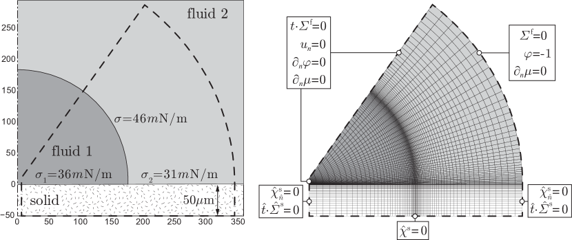
Figure 1: Illustration of the considered experimental configuration (left) and the corresponding computational setup (right).

We incorporate the rotational symmetry of the experimental setup in the discrete approximation of (19). The considered approximation spaces are based on a locally refined mesh, adapted to the diffuse interface; see Fig. 1 (right). We apply Raviart-Thomas compatible B-spline approximations for velocity ($u$) and pressure ($p$) with order $((3,2),(2,3))$ and $2$, respectively; see [7, 9]. The order parameter ($\varphi$) and chemical potential ($\mu$) are approximated by means of quadratic B-splines. The solid deformation ($\hat{\chi}^{\mathrm{s}}$) and the deformation of the fluid domain ($\smash[tb]{\hat{\chi}^{\mathrm{f}}}$) are approximated with quadratic B-splines as well. Let us note that by virtue of the $C^{1}$-continuity of the solid deformation, the interface $\Gamma_{t}$ corresponds to a $C^{1}$ manifold. The temporal discretization of (19) is based on backward Euler approximation of the time derivatives, with time step $0.5\,m\mathrm{s}$. In each time step, the aggregated fluid-solid interaction problem is solved by means of subiteration with underrelaxation; see, for instance, [5].

Figure 2 (left) presents a comparison of the computed interface configuration, $\Gamma_{t}$, at $t\in\{0,0.5,1,2,4,8,16\}\,m\mathrm{s}$ and experimental data from [18]. At $t=16\,m\mathrm{s}$, the interface has essentially reached its equilibrium deformation. The surface tension of the fluid-fluid interface yields a localized load on the fluid-solid interface near the contact line, resulting in a kink in the surface deformation of the soft substrate. In addition, the fluid-fluid surface tension leads to an increased pressure in the droplet relative to the ambient pressure (see also Fig. 2 (right)), viz. Laplace pressure, and a corresponding depression of the substrate. Comparison of the experimental and computed results conveys that the fluid-solid interface elevation at the contact line is underestimated by approximately 25$\%$. The underestimation can be attributed to the regularizing effect of the diffuse interface. It is anticipated that further reduction of the diffuse-interface thickness ($\epsilon$) and corresponding refinement of the mesh leads to an increase in the fluid-solid interface elevation at the contact line. The indentation of the substrate below the droplet is noticeably overestimated. In this regard, it is to be mentioned that on account of the nearly incompressible behavior of the solid, its volume at $t=16\,m\mathrm{s}$ has decreased by only $0.16\%$ relative to the initial volume.

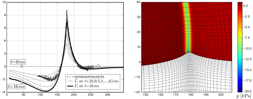
Figure 2: Comparison of the computed fluid-solid-interface configuration $\Gamma_{t}$ at $t\in\{0,0.5,1,2,4,8\}\,m\mathrm{s}$ (grey) and at $t=16\,m\mathrm{s}$ (black) and rendering of experimental results from [18] (left), and magnification of the contact-line region at $t=16\,m\mathrm{s}$ with deformed fluid and solid meshes and computed pressure distribution (right).

Figure 2 (right) presents a magnification of the contact-line region at $t=16\,m\mathrm{s}$ with the fluid and solid meshes in the actual configuration and the computed pressure distribution in the complex fluid. It is noteworthy that the pressure in the diffuse interface exhibits a localized minimum at the contact line. The pressure in the droplet is virtually uniform with value $p\approx{}520\,\mathrm{Pa}$, which is close to the theoretical Laplace pressure $2\sigma/R$ in a droplet on a rigid substrate with radius $R=178\,\mu\mathrm{m}$ and surface tension $\sigma=46\,m\,\mathrm{N}/\mathrm{m}$.

0.5 Conclusion

We presented a model for the interaction of a complex fluid with an elastic solid, in which the complex fluid is represented by the Navier–Stokes–Cahn–Hilliard (NSCH) equations and the solid is characterized by a hyperelastic material with a Saint Venant–Kirchhoff stored-energy functional. The interaction between the fluid and the solid at their mutual interface is described by a preferential-wetting condition in addition to the usual kinematic and dynamic interface conditions. The fluid traction on the fluid-solid interface comprises a non-standard capillary-stress contribution, and the dynamic condition contains a contribution from the non-uniform fluid-solid surface tension. A weak formulation of the complex-fluid-solid-interaction (CFSI) problem was presented, based on an ALE formulation of the NSCH system and a suitable reformulation of the complex-fluid traction and the fluid-solid surface-tension traction.

Numerical results were presented for a stationary droplet on a soft solid substrate, based on finite-element approximation of the weak formulation of the aggregated CFSI problem. Comparison of the computed results with experimental data for the considered test case exhibited very good agreement in the contact-line region. The substrate depression below the droplet was noticeably overestimated relative to the experimental data. In view of the close agreement between the computed pressure in the droplet and the theoretical Laplace pressure, it appears that the discrepancy between the computed and observed depression is to be attributed to corresponding differences in the constitutive behavior of the solid substrate. The overall good agreement between the computed and experimental data indicates the potential of computational CFSI models based on the NSCH equations to predict elasto-capillary phenomena.

References

- [1] H. Abels, H. Garcke, and G. Grün. Thermodynamically consistent, frame indifferent diffuse interface models for incompressible two-phase flows with different densities. Mathematical Models and Methods in Applied Sciences, 22:1150013, 2012.
- [2] S. Aland and A. Voigt. Benchmark computations of diffuse interface models for two-dimensional bubble dynamics. Int. J. Numer. Meth. Fluids, 69:747–761, 2012.
- [3] E. Bänsch. Finite element discretization of the navier–stokes equations with a free capillary surface. Numer. Math., 88:203–235, 2001.
- [4] Y. Bazilevs, K. Takizawa, and T.E. Tezduyar. Computational Fluid-Structure Interaction: Methods and Applications. Wiley, 2013.
- [5] E.H. van Brummelen. Partitioned iterative solution methods for fluid-structure interaction. Int. J. Numer. Meth. Fluids, 65:3–27, 2011.
- [6] J. Bueno, C. Bona-Casas, Y. Bazilevs, and H. Gomez. Interaction of complex fluids and solids: theory, algorithms and application to phase-change-driven implosion. Comput. Mech., pages 1–14, 2014.
- [7] A. Buffa, C. de Falco, and G. Sangalli. Isogeometric analysis: Stable elements for the 2D stokes equation. International Journal for Numerical Methods in Fluids, 65(11-12):1407–1422, 2011.
- [8] G. Dziuk. An algorithm for evolutionary surfaces. Numer. Math., 58:603–611, 1991.
- [9] J.A. Evans and T.J.R. Hughes. Isogeometric divergence-conforming b-splines for the steady Navier-Stokes equations. Mathematical Models and Methods in Applied Sciences, 23:1421–1478, 2012.
- [10] H. Gouin. Interfaces endowed with nonconstant surface energies revisited with the d’Alembert–Lagrange principle. Mathematics and Mechanics of Complex Systems, 2:23–43, 2014.
- [11] Z. Guo, P. Lin, and J.S. Lowengrub. A numerical method for the quasi-incompressible cahn–hilliard–navier–stokes equations for variable density flows with a discrete energy law. J. Comput. Phys., 276:486–507, 11 2014.
- [12] P.C. Hohenberg and B.I. Halperin. Theory of dynamic critical phenomena. Rev. Mod. Phys., 49:435–479, 1977.
- [13] D. Jacqmin. Calculation of two-phase navier-stokes flows using phase-field modeling. Journal of Computational Physics, 155(1):96–127, 10 1999.
- [14] D. Jacqmin. Contact-line dynamics of a diffuse fluid interface. Journal of Fluid Mechanics, 402:57–88, 2000.
- [15] J. Lowengrub and L. Truskinovsky. Quasi-incompressible Cahn-Hilliard fluids and topological transitions. Proceedings: Mathematical, Physical and Engineering Sciences, 454(1978):2617–2654, 10 1998.
- [16] H. Melbø and T. Kvamsdal. Goal oriented error estimators for Stokes equations based on variationally consistent postprocessing. Comput. Methods Appl. Mech. Engrg., 192:613–633, 2003.
- [17] C. Py, P. Reverdy, L. Doppler, J. Bico, B. Roman, and C.N. Baroud. Capillary origami: Spontaneous wrapping of a droplet with an elastic sheet. Phys. Rev. Lett., 98:156103, Apr 2007.
- [18] R.W. Style, R. Boltyanskiy, Y. Che, J.S. Wettlaufer, L.A. Wilen, and E.R. Dufresne. Universal deformation of soft substrates near a contact line and the direct measurement of solid surface stresses. Phys. Rev. Lett., 110:066103, Feb 2013.
- [19] R.W. Style et al. Patterning droplets with durotaxis. PNAS, 110(31):12541–12544, 2013.
- [20] T.E. Tezduyar, K. Takizawa, C. Moorman, S. Wright, and J. Christopher. Space–time finite element computation of complex fluid–structure interactions. Int. J. Numer. Meth. Fluids, 64:1201–1218, 2010.
- [21] E.H. van Brummelen, K.G. van der Zee, V.V. Garg, and S. Prudhomme. Flux evaluation in primal and dual boundary-coupled problems. J. Appl. Mech., 79:010904–8, 2012.
- [22] K.G. van der Zee, E.H. van Brummelen, I. Akkerman, and R. de Borst. Goal-oriented error estimation and adaptivity for fluid-structure interaction using exact linearized adjoints. Comput. Methods Appl. Mech. Engrg., 200:2738–2757, 2011.