Zero forcing and power domination for graph products

Abstract

The power domination number arises from the monitoring of electrical networks and its determination is an important problem. Upper bounds for power domination numbers can be obtained by constructions. Lower bounds for the power domination number of several families of graphs are known, but they usually arise from specific properties of each family and the methods do not generalize. In this paper we exploit the relationship between power domination and zero forcing to obtain the first general lower bound for the power domination number. We apply this bound to obtain results for both the power domination of tensor products and the zero-forcing number of lexicographic products of graphs. We also establish results for the zero forcing number of tensor products and Cartesian products of graphs.

Keywords power domination, zero forcing, maximum nullity, minimum rank, tensor product, lexicographic product, Cartesian product

AMS subject classification 05C69, 05C50

1 Introduction

Electric power companies need to monitor the state of their networks continuously. One method of monitoring a network is to place Phase Measurement Units (PMUs) at selected locations in the system, called electrical nodes or buses, where transmission lines, loads, and generators are connected. A PMU placed at an electrical node measures the voltage at the node and all current phasors at the node [2]; it also provides these measurements at other vertices or edges according to certain propagation rules (see Section 1.3 for the formal definitions of this and other terms). The placement of PMUs at all nodes of a network is a trivial solution to the monitoring problem. Because of the cost of a PMU, the trivial solution is not feasible, and it is important to minimize the number of PMUs used while maintaining the ability to observe the entire system.

This problem was first studied in terms of graphs by Haynes et al. in [13]. Indeed, an electric power network can be modeled by a graph where the vertices represent the electric nodes and the edges are associated with the transmission lines joining two electrical nodes. In this model, the power domination problem in graphs consists of finding a minimum set of vertices from where the entire graph can be observed according to certain rules. In terms of the physical network, such a minimum set of vertices will provide the locations where the PMUs should be placed in order to monitor the entire graph at minimum cost. Since its introduction in [13], the power domination number and variations have generated considerable interest (see, for example, [4, 5, 8, 9, 10, 17, 19]).

As was pointed out in [8], a careful examination of the definition of power domination leads naturally to the study of zero forcing. The zero forcing number was introduced in [1] as an upper bound for the maximum nullity of real symmetric matrices whose nonzero pattern of off-diagonal entries is described by a given graph, and independently by mathematical physicists studying control of quantum systems.

In Section 3 we use the connection between the two definitions established in [8] to obtain the only known general lower bound for the power domination number. Note that in [17] the author claimed to have obtained the first general lower bound for the power domination number, but a family of counterexamples to his claim was given in [12]. Then we use our lower bound to prove results for both power domination and zero forcing. Some of these applications require additional knowledge of zero forcing numbers of tensor products, which we establish in Section 2.1, via a new upper bound on the zero forcing number of the tensor product of a complete graph with another graph. The remainder of this introduction contains formal definitions of power domination and zero forcing, graph terminology, and matrix terminology.

1.1 Power domination and zero forcing definitions

A graph $G=(V,E)$ is an ordered pair formed by a finite nonempty set of vertices $V=V(G)$ and a set of edges $E=E(G)$ containing unordered pairs of distinct vertices (that is, all graphs are simple and undirected). The order of $G$ is denoted by $|G|:=|V(G)|$. We say the vertices $u$ and $v$ are adjacent or are neighbors, and write $u\sim v$, if $\{u,v\}\in E$. For any vertex $v\in V$, the neighborhood of $v$ is the set $N(v)=\{u\in V:u\sim v\}$ (or $N_{G}(v)$ if $G$ is not clear from context), and the closed neighborhood of $v$ is the set $N[v]=N(v)\cup\{v\}$. Similarly, for any set of vertices $S$, $N(S)=\cup_{v\in S}N(v)$ and $N[S]=\cup_{v\in S}N[v]$.

A vertex $v$ in a graph $G$ is said to dominate itself and all of its neighbors in $G$. A set of vertices $S$ is a dominating set of $G$ if every vertex of $G$ is dominated by a vertex in $S$. The minimum cardinality of a dominating set is the domination number of $G$ and is denoted by $\gamma(G)$.

In [13] the authors introduced the related concept of power domination by presenting propagation rules in terms of vertices and edges in a graph. In this paper we will use a simplified version of the propagation rules that is equivalent to the original, as shown in [4]. For a set $S$ of vertices in a graph $G$, define $PD(S)\subseteq V(G)$ recursively:

1. $PD(S):=N[S]=S\cup N(S)$.

2. While there exists $v\in PD(S)$ such that $|N(v)\cap(V(G)\setminus PD(S))|=1$:

   $PD(S):=PD(S)\cup N(v)$.

We say that a set $S\subseteq V(G)$ is a power dominating set of a graph $G$ if at the end of the process above $PD(S)=V(G)$. A minimum power dominating set is a power dominating set of minimum cardinality, and the power domination number $\gamma_{P}(G)$ of $G$ is the cardinality of a minimum power dominating set.

The concept of zero forcing can be explained via a coloring game on the vertices of $G$. The color change rule is: If $u$ is a blue vertex and exactly one neighbor $w$ of $u$ is white, then change the color of $w$ to blue. We say $u$ forces $w$ and denote this by $u\to w$. A zero forcing set for $G$ is a subset of vertices $B$ such that when the vertices in $B$ are colored blue and the remaining vertices are colored white initially, repeated application of the color change rule can color all vertices of $G$ blue. A minimum zero forcing set is a zero forcing set of minimum cardinality, and the zero forcing number $\operatorname{Z}(G)$ of $G$ is the cardinality of a minimum zero forcing set. The next observation is the key relationship between the two concepts.

Observation 1.1.

[8] The power domination process on a graph $G$ can be described as choosing a set $S\subseteq V(G)$ and applying the zero forcing process to the closed neighborhood $N[S]$ of $S$. The set $S$ is a power dominating set of $G$ if and only if $N[S]$ is a zero forcing set for $G$.

The degree of a vertex $v$, denoted by $\deg v$, is the cardinality of the set $N(v)$. The maximum and minimum degree of $G$ are defined as $\Delta(G)=\max\{\deg v:v\in V\}$ and $\delta(G)=\min\{\deg v:v\in V\}$, respectively. A graph $G$ is regular if $\delta(G)=\Delta(G)$.

The next observation is well known (and immediate since the color change rule cannot be applied in $G$ without at least $\delta(G)$ blue vertices).

Observation 1.2.

For every graph $G$, $\delta(G)\leq\operatorname{Z}(G)$.

1.2 Graph definitions and notation

Let $n$ be a positive integer. The path of order $n$ is the graph $P_{n}$ with $V(P_{n})=\{x_{i}:1\leq i\leq n\}$ and $E(P_{n})=\{\{x_{i},x_{i+1}\}:1\leq i\leq n-1\}$. If $n\geq 3$, the cycle of order $n$ is the graph $C_{n}$ with $V(C_{n})=\{x_{i}:1\leq i\leq n\}$ and $E(C_{n})=\left\{\left\{x_{i},x_{i+1}\right\}:1\leq i\leq n-1\right\}\cup\left\{\{x_{n},x_{1}\}\right\}$. The complete graph of order $n$ is the graph $K_{n}$ with $V(K_{n})=\{x_{i}:1\leq i\leq n\}$ and $E(K_{n})=\{\{x_{i},x_{j}\}:1\leq i<j\leq n\}$.

Let $G=(V(G),E(G))$ and $H=(V(H),E(H))$ be disjoint graphs. All of the following products of $G$ and $H$ have vertex set $V(G)\times V(H)$. The tensor product (also called the direct product) of $G$ and $H$ is denoted by $G\times H$; a vertex $(g,h)$ is adjacent to a vertex $(g^{\prime},h^{\prime})$ in $G\times H$ if $\{g,g^{\prime}\}\in E(G)$ and $\{h,h^{\prime}\}\in E(H)$. The Cartesian product of $G$ and $H$ is denoted by $G\,\Box\,H$; two vertices $(g,h)$ and $(g^{\prime},h^{\prime})$ are adjacent in $G\,\Box\,H$ if either (1) $g=g^{\prime}$ and $\{h,h^{\prime}\}\in E(H)$, or (2) $h=h^{\prime}$ and $\{g,g^{\prime}\}\in E(G)$. The lexicographic product of $G$ and $H$ is denoted by $G*H$; two vertices $(g,h)$ and $(g^{\prime},h^{\prime})$ are adjacent in $G*H$ if either (1) $\{g,g^{\prime}\}\in E(G)$, or (2) $g=g^{\prime}$ and $\{h,h^{\prime}\}\in E(H)$. Note that $H\times G\cong G\times H$ and $H\,\Box\,G\cong G\,\Box\,H$, whereas $H*G$ need not be isomorphic to $G*H$.

For a graph $G$ with no edges, $\operatorname{Z}(G)=\gamma_{P}(G)=\gamma(G)=|G|$, so we focus our attention on graphs with edges. In the case of the tensor product $G\times H$, this means we assume $|G|,|H|\geq 2$.

1.3 Matrix definitions and notation

Let $S_{n}(\mathbb{R})$ denote the set of all $n\times n$ real symmetric matrices. For $A=[a_{ij}]\in S_{n}(\mathbb{R})$, the graph of $A$, denoted by $\mathcal{G}(A)$, is the graph with vertices $\{1,\ldots,n\}$ and edges $\{\{i,j\}:a_{ij}\not=0,\,1\leq i<j\leq n\}$. More generally, the graph of $A$ is defined for any matrix that is combinatorially symmetric, i.e., $a_{ij}=0$ if and only if $a_{ji}=0$. Note that the diagonal of $A$ is ignored in determining $\mathcal{G}(A)$. The set of symmetric matrices described by a graph $G$ of order $n$ is defined as $\mathcal{S}(G)=\{A\in S_{n}(\mathbb{R}):\mathcal{G}(A)=G\}$. The maximum nullity of $G$ is $\operatorname{M}(G)=\max\{\operatorname{null}A:A\in\mathcal{S}(G)\}$, and the minimum rank of $G$ is $\operatorname{mr}(G)=\min\{{\rm rank}\,A:A\in S(G)\}$; clearly $\operatorname{M}(G)+\operatorname{mr}(G)=|G|$. The term ‘zero forcing’ comes from using the forcing process to force zeros in a null vector of a matrix $A\in\mathcal{S}(G)$, implying $\operatorname{M}(G)\leq\operatorname{Z}(G)$ [1].

A standard way to construct matrices of maximum nullity for a Cartesian product or a tensor product of graphs is to use the Kronecker or tensor product of matrices. Let $A$ be an $n\times n$ real matrix and $B$ be an $m\times m$ real matrix. Then $A\otimes B$ is the $n\times n$ block matrix whose $ij$th block is the $m\times m$ matrix $a_{ij}B$. It is known that $(A\otimes B)^{T}=A^{T}\otimes B^{T}$ and $\operatorname{rank}(A\otimes B)=(\operatorname{rank}A)(\operatorname{rank}B)$. If $A\in\mathcal{S}(G)$, $B\in\mathcal{S}(H)$, $|G|=n$, and $|H|=m$, then $A\otimes I_{m}-I_{n}\otimes B\in\mathcal{S}(G\,\Box\,H)$. If ${\bf x}$ is an eigenvector of $A$ for eigenvalue $\lambda$ and ${\bf y}$ is an eigenvector of $B$ for eigenvalue $\mu$, then ${\bf x}\otimes{\bf y}$ is an eigenvector of $A\otimes I_{m}-I_{n}\otimes B$ for eigenvalue $\lambda-\mu$. Since a real symmetric matrix has a full set of eigenvectors, the multiplicity of $\lambda-\mu$ is $\operatorname{mult}_{A}(\lambda)\,\operatorname{mult}_{B}(\mu)$ [1, Observation 3.5]. If $A\in\mathcal{S}(G)$ and $B\in\mathcal{S}(H)$ and the diagonal entries of $A$ and $B$ are all zero, then $A\otimes B\in\mathcal{S}(G\times H)$. Define $\mathcal{M}_{0}(G)=\{A\in\mathbb{R}^{n\times n}:\mathcal{G}(A)=G\mbox{ and $a_{ii}=0$ for }i=1,\dots,n\}$; in contrast to a matrix in $\mathcal{S}(G)$, a matrix in $\mathcal{M}_{0}(G)$ need not be symmetric but must have a zero diagonal and be combinatorially symmetric. If $A\in\mathcal{M}_{0}(G)$ and $B\in\mathcal{M}_{0}(H)$, then $A\otimes B\in\mathcal{M}_{0}(G\times H)$.

2 Zero forcing for graph products

In this section we develop a tool for the zero forcing number of tensor products of graphs and apply it to compute the tensor products of complete graphs with paths and with cycles. We also compute the zero forcing number and maximum nullity of the Cartesian product of two cycles.

2.1 Tensor products

For tensor products of graphs we use not only standard zero forcing, but also skew zero forcing [16] defined by the skew color change rule: If a vertex $v$ of $G$ has exactly one white neighbor $w$, then $v$ forces $w$ to change color to blue; if $v$ is white when it forces, the force $v\to w$ is called a white vertex force. The skew zero forcing number, $\operatorname{Z}^{-}(G)$, is the minimum cardinality of a skew zero forcing set, i.e., a (possibly empty) set of blue vertices that can color all vertices blue using the skew color change rule. Note that we are using skew zero forcing as a tool, and it is not directly connected to power domination. For either a standard or skew zero forcing set $B$, color all the vertices of $B$ blue and then perform zero forcing, listing the forces in the order in which they were performed. This list is a chronological list of forces of $B$ and is denoted by $\mathcal{F}$.

For each vertex $g\in V(G)$, define the set $U_{g}=\{(g,h):h\in V(H)\}$ in $G\times H$. We say vertices $(g,h)$ and $(g^{\prime},h)$ are associates in $G\times H$ if $g\sim g^{\prime}$ in $G$; associates are not adjacent in $G\times H$.

Theorem 2.1.

Let $G$ be a graph and $n\geq 4$. Then

$$\operatorname{Z}(G\times K_{n})\leq(n-2)|G|+2\operatorname{Z}^{-}(G).$$

Proof.

For $g\sim g^{\prime}$ in $G$, $(g,i)\sim(g^{\prime},j)$ in $G\times K_{n}$ for all $j\neq i\in V(K_{n})$. Choose a minimum skew zero forcing set $B$ for $G$ and a chronological list of forces $\mathcal{F}$ of $B$ and denote the $k$th force by $g_{k}\to w_{k}$ (many vertices receive two labels, e.g., $g_{k}=w_{\ell}$). We describe how to choose $(n-2)|G|+2|B|$ vertices to obtain a zero forcing set $\hat{B}$ for $G\times K_{n}$. For $g\in B$, let $\hat{B}\supset U_{g}$. For $v\not\in B$, place $n-2$ vertices of $U_{v}$ in $\hat{B}$; the selection of these vertices is determined when $v$ is forced in $G$ or when $v$ performs a force in $G$, whichever comes first.

Consider the $k$th force in $\mathcal{F}$ ($k=1$ is permitted). Suppose $g_{k}\to w_{k}$ is not a white vertex force. If no vertices of $U_{w_{k}}$ are in $\hat{B}$ yet, then arbitrarily choose $n-2$ vertices in $U_{w_{k}}$ to place in $\hat{B}$; otherwise, no additional vertices are placed in $\hat{B}$. Now suppose $g_{k}\to w_{k}$ is a white vertex force. Clearly, $w_{k}\not\in B$ and $w_{k}$ has not been forced previously in $G$. The only force ${w_{k}}$ could have performed in $G$ would be $w_{k}\to{g_{k}}$, in which case $g_{k}\to w_{k}$ would not be a white vertex force. Thus, no vertices in $U_{w_{k}}$ have been previously placed in $\hat{B}$. Also, no vertices of $U_{g_{k}}$ have been previously placed in $\hat{B}$. Since $n\geq 4$, it is possible to choose $n-2$ vertices in each of $U_{g_{k}}$ and $U_{w_{k}}$, and place in $\hat{B}$, in such a way that for every pair of associated vertices in $U_{g_{k}}$ and $U_{w_{k}}$, at least one member of the pair is placed in $\hat{B}$. By construction, $|\hat{B}|=|B|n+(|G|-|B|)(n-2)$.

The zero forcing process in $G\times K_{n}$ now follows the chronological list of forces $\mathcal{F}$. At stage $k$ (before performing the $k$th force), we assume every vertex in $U_{v}$ is blue for every $v$ such that $v\in B$ or $v=w_{\ell}$ with $\ell<k$. Given the force $g_{k}\to w_{k}$ in $\mathcal{F}$, the two (blue) vertices in $U_{g_{k}}$ that are associated with the two white vertices in $U_{w_{k}}$ can each force the other’s associate in $U_{w_{k}}$, so $U_{w_{k}}$ is now entirely blue. Thus, all sets $U_{w_{k}}$ will be turned entirely blue. ∎

The forcing process used in the proof of Theorem 2.1 is illustrated in Figure 1, where skew forcing is shown on $P_{6}$ and standard zero forcing is shown on $P_{6}\times K_{5}$; the number of each force in a chronological list of forces of $P_{6}$ is also shown. The first half of the forces in $P_{6}$ (forces 1, 2, and 3) are white vertex forces and the second half are not.

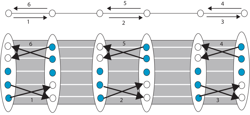
Figure 1: The skew zero forcing process on $P_{6}$ and the analogous zero forcing process on $P_{6}\times K_{5}$ are illustrated. In the schematic diagram of $P_{6}\times K_{5}$, the gray areas indicate that all possible edges are present except for the non-edges marked as white lines.

Note that the bound in Theorem 2.1 need not be valid for $n=3$, as shown in the next example.

Example 2.2.

Let $H_{3}$ denote the 3-sun shown in Figure 2 and consider $H_{3}\times K_{3}$. Suppose $\hat{B}$ is a zero forcing set for $H_{3}\times K_{3}$ of cardinality six. Observe that $\hat{B}$ must contain at least one vertex in $U_{g}$ for each $g\in V(H_{3})$, or no vertices in $U_{g}$ could ever be colored blue, so necessarily $\hat{B}$ contains exactly one vertex of each $U_{g}$. In $H_{3}\times K_{3}$ there are three sets $U_{g}$ that contain vertices of degree 2 (corresponding to the three vertices of degree 1 in $H_{3}$) and three sets of vertices of degree 6. With appropriately staggered choices of which vertex of $U_{g}$ is in $\hat{B}$, each of the three blue vertices of degree 2 can force one degree 6 vertex blue. Now the only blue vertices that have not yet forced all have degree 6. Each has (at least) one white neighbor of degree 2. In order for such vertex to perform a force, it must have no other white neighbors. That is, all four of its degree 6 neighbors must be blue. This implies two degree 6 white vertices must be associates, preventing any further forcing. Thus $\operatorname{Z}(H_{3}\times K_{3})\geq 7>6=(3-2)6+0$ and $\operatorname{Z}^{-}(H_{3})=0$. (The zero forcing number of this example was originally found by use of the Sage zero forcing software [18], which found a zero forcing set of order 7 and determined no smaller ones exist.)

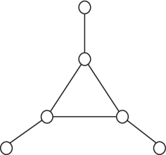
Figure 2: The 3-sun

We apply Theorem 2.1 to the tensor product of a path and a complete graph. The case of odd paths has already been done:

Theorem 2.3.

[15, Theorem 15] If $t\geq 1$ is odd and $n\geq 2$, then $M(P_{t}\times K_{n})=Z(P_{t}\times K_{n})=(n-2)t+2$.

The method used to prove [15, Theorem 15] is the standard one of exhibiting a matrix and a zero forcing set with cardinality equal to the nullity of the matrix. For even paths, we use the same matrix to establish a lower bound on maximum nullity. For $n\geq 4$, Theorem 2.1 gives an equal upper bound on the zero forcing number; a specific zero forcing set is exhibited for $n=3$.

Theorem 2.4.

If $t\geq 2$ is even and $n\geq 3$, then

$$\operatorname{M}(P_{t}\times K_{n})=\operatorname{Z}(P_{t}\times K_{n})=(n-2)t.$$

Proof.

Define the $n$-vectors $\mathds{1}=[1,1,\dots,1]^{T}$ and ${\bf y}=[1,2,\dots,n]^{T}$, and define $A_{n}=[\mathds{1}\,{\bf y}]\begin{bmatrix}0&1\\ -1&0\end{bmatrix}\begin{bmatrix}\mathds{1}^{T}\\ {\bf y}^{T}\end{bmatrix}$. Then $\operatorname{rank}A_{n}=2$, $A_{n}^{T}=-A_{n}$, and $A_{n}\in\mathcal{M}_{0}(K_{n})$. Define $B_{t}$ to be a $t\times t$ skew adjacency matrix (a tridiagonal matrix with 1s on the first superdiagonal, 0s on the main diagonal, and $-1$s on the first subdiagonal); note that since $t$ is even, $\operatorname{rank}B_{t}=t$. Then $B_{t}\otimes A_{n}\in\mathcal{S}(P_{t}\times K_{n})$ and $\operatorname{rank}(B_{t}\otimes A_{n})=2t$. Thus $(n-2)t=tn-2t\leq\operatorname{M}(P_{t}\times K_{n})\leq\operatorname{Z}(P_{t}\times K_{n})$. For $n\geq 4$, $\operatorname{Z}(P_{t}\times K_{n})\leq(n-2)t$ by Theorem 2.1, since $\operatorname{Z}^{-}(P_{t})=0$ for $t$ even [16].

Now assume $n=3$. The forcing order in $P_{t}\times K_{3}$ is slightly more complicated than the one in Theorem 2.1, since initially only a single vertex can force at a time. Label the vertices of $P_{t}\times K_{3}$ as ordered pairs $(r,s)$ with $1\leq r\leq t$ and $1\leq s\leq 3$. Define $B=\{(2i-1,3),(2i,1):i=1,\dots,\frac{t}{2}\}$. First, $(1,3)$ forces $(2,2)$. Continue in increasing order of sets, so $(2i-1,3)$ forces $(2i,2)$ for $i=1,\dots,\frac{t}{2}$. Then the process is repeated in reverse order, starting at $2i=t$. Now, $(t,1)$ and $(t,2)$ are both blue with one white neighbor each, so $(t,1)$ forces $(t-1,2)$ and $(t,2)$ forces $(t-1,1)$. Continue in decreasing order, so $(2i,1)$ forces $(2i-1,2)$ and $(2i,2)$ forces $(2i-1,1)$ for $i=\frac{t}{2}$ down to $i=1$, turning all odd-numbered sets all blue. Finally, in increasing order again, $(2i-1,2)$ forces $(2i,3)$ for $i=1,\dots,\frac{t}{2}$. ∎

Observe that the formula in Theorem 2.4 fails for $n=2$: $P_{t}\times K_{2}$ is the disjoint union of two copies of $P_{2}$, so $\operatorname{M}(P_{t}\times K_{2})=\operatorname{Z}(P_{t}\times K_{2})=2\neq(2-2)t$.

Theorem 2.5.

If $n,t\geq 3$, then

$$\operatorname{M}(C_{t}\times K_{n})=\operatorname{Z}(C_{t}\times K_{n})=\left\{\begin{array}[]{ll}(n-2)t+2&\mbox{ if $t$ is odd,}\\ (n-2)t+4&\mbox{ if $t$ is even.}\end{array}\right.$$

Proof.

Let the matrix $A_{n}$ be as defined in the proof of Theorem 2.4, so $\operatorname{rank}A_{n}=2$, $A_{n}^{T}=-A_{n}$, and $A_{n}\in\mathcal{M}_{0}(K_{n})$. Define $B_{t}$ to be the $t\times t$ skew-adjacency matrix (with 1s in one cyclic direction and $-1$s in the other). It is easy to verify that $\det B_{t}=0$, $\operatorname{rank}B_{t}=t-1$ for $t$ odd, and $\operatorname{rank}B_{t}=t-2$ for $t$ even. Then $B_{t}\otimes A_{n}\in\mathcal{S}(C_{t}\times K_{n})$ and

$$\operatorname{rank}(B_{t}\otimes A_{n})=\left\{\begin{array}[]{ll}2t-2&\mbox{ if $t$ is odd,}\\ 2t-4&\mbox{ if $t$ is even.}\end{array}\right.$$

Since $\operatorname{M}(C_{t}\times K_{n})\leq\operatorname{Z}(C_{t}\times K_{n})$, it suffices to exhibit a zero forcing set of cardinality $(n-2)t+2$ for $t$ odd and $(n-2)t+4$ for $t$ even. Color all the vertices in $U_{t}$ blue for $t$ odd, or all the vertices in $U_{t-1}$ and in $U_{t}$ blue for $t$ even. We now consider the graph obtained by deleting these blue vertices, i.e., $P_{t-1}\times K_{n}$ or $P_{t-2}\times K_{n}$, respectively, both having the form of a tensor product of an even path with a complete graph. We construct a minimum zero forcing set $\hat{B}^{\prime}$ (of cardinality $(n-2)(t-1)$ or $(n-2)(t-2)$, respectively) and perform zero forcing for the tensor product of an even path and a complete graph as in Theorem 2.4. The zero forcing set for $C_{t}\times K_{n}$ is $\hat{B}^{\prime}\cup U_{t}$ or $\hat{B}^{\prime}\cup U_{t}\cup U_{t-1}$, respectively. ∎

2.2 Cartesian products

Next we determine the zero forcing number and maximum nullity of the Cartesian product of two cycles.

Theorem 2.6.

For $m\geq n\geq 3$,

$$\operatorname{M}(C_{n}\,\Box\,C_{m})=\operatorname{Z}(C_{n}\,\Box\,C_{m})=\left\{\begin{array}[]{ll}2n-1&\mbox{ if $m=n$ and $n$ is odd,}\\[2.84526pt] 2n&\mbox{ otherwise.}\end{array}\right.$$

Proof.

For $m=n\geq 3$, by [7, Theorem 2.18] $\operatorname{M}(C_{n}\,\Box\,C_{n})=\operatorname{Z}(C_{n}\,\Box\,C_{n})=n+2\left\lfloor\frac{n}{2}\right\rfloor$, so $\operatorname{M}(C_{n}\,\Box\,C_{n})=\operatorname{Z}(C_{n}\,\Box\,C_{n})=2n-1$ for $n$ odd and $\operatorname{M}(C_{n}\,\Box\,C_{n})=\operatorname{Z}(C_{n}\,\Box\,C_{n})=2n$ for $n$ even.

So assume $m>n\geq 3$. It is easy to see that the vertices of two consecutive cycles $C_{n}$ form a zero forcing set, so $\operatorname{Z}(C_{n}\,\Box\,C_{m})\leq 2n$. To complete the proof we construct a matrix in $\mathcal{S}(C_{n}\,\Box\,C_{m})$ with nullity $2n$, so $2n\leq\operatorname{M}(C_{n}\,\Box\,C_{m})\leq\operatorname{Z}(C_{n}\,\Box\,C_{m})\leq 2n$.

Let $k=\left\lceil\frac{n}{2}\right\rceil$. Let $A$ be the matrix obtained from the adjacency matrix of $C_{n}$ by changing one pair of symmetrically placed entries from 1 to $-1$. Then the distinct eigenvalues of $A$ are $\mu_{i}=2\cos\frac{\pi(2i-1)}{n},$ $i=1,\dots,{k}$, each with multiplicity 2 except $\mu_{k}=-2$, which has multiplicity 1 when $n$ is odd [1, Theorem 3.8]. Assuming that there exists a matrix $B\in\mathcal{S}(C_{m})$ such that $\mu_{i}$ is an eigenvalue of $B$ with multiplicity 2 for $i=1,\dots,k$, it follows that $A\otimes I_{m}-I_{n}\otimes B$ has eigenvalue zero with multiplicity $2n$, because every eigenvalue of $A$ has a corresponding eigenvalue of $B$ with multiplicity 2.

It remains to establish the existence of a matrix $B\in\mathcal{S}(C_{m})$ such that $\mu_{i}$ is an eigenvalue of $B$ with multiplicity 2 for $i=1,\dots,k$. In Ferguson [11, Theorem 4.3] it is shown that for any set of $m$ real numbers $\lambda_{1}>\lambda_{2}\geq\lambda_{3}>\lambda_{4}\geq\lambda_{5}>\dots$, there is a matrix $B\in\mathcal{S}(C_{m})$ having eigenvalues $\lambda_{1},\dots,\lambda_{m}$. Thus for $m$ odd or $m\geq n+2$ we can choose $\lambda_{2i}=\lambda_{2i+1}=\mu_{i}$. Hall [14] showed that for $m=2k$ and any $\lambda_{1}>\lambda_{2}>\dots>\lambda_{k}$ there is a matrix $B\in\mathcal{S}(C_{m})$ with $\operatorname{mult}_{B}(\lambda_{i})=2$ for $i=1,\dots,k$. ∎

3 Zero forcing lower bound for power domination number

The power domination number of several families of graphs has been determined using a two-step process: finding an upper bound and a lower bound. The upper bound is usually obtained by providing a pattern to construct a set, together with a proof that the constructed set is a power dominating set. The lower bound is usually found by exploiting structural properties of the particular family of graphs, and it often consists of a very technical and lengthy process (see, for example, [10]). Therefore, finding good general lower bounds for the power domination number is an important problem.

An effort in that direction is the work by Stephen et al. [19, Theorem 3.1] in which a lower bound is presented and successfully applied to finding the power domination number of some graphs modeling chemical structures. However, their lower bound depends heavily on the choice of a family of subgraphs satisfying certain properties. While in some graphs it is possible to find families of subgraphs that yield good lower bounds, in others it is not, and the bound depends on the family of subgraphs chosen rather than on the graph itself.

The lower bound for the power domination number of a hypercube presented in Dean et al. [8] is based on the following result:

Theorem 3.1.

[8, Lemma 2] Let $G$ be a graph with no isolated vertices, and let $S=\{u_{1},\dots,u_{t}\}$ be a power dominating set for $G$. Then $\operatorname{Z}(G)\leq\sum_{i=1}^{t}\deg u_{i}.$

While Dean et al. only apply Theorem 3.1 to the study of a particular family of graphs, Theorem 3.1 is the starting point in our process to obtain a general lower bound. The next theorem, which follows from Theorem 3.1, can be used to map zero forcing results to power dominating results and vice versa.

Theorem 3.2.

Let $G$ be a graph that has an edge. Then $\left\lceil\frac{\operatorname{Z}(G)}{\Delta(G)}\right\rceil\leq\gamma_{P}(G)$, and this bound is tight.

Proof.

Choose a minimum power dominating set $\{u_{1},\dots,u_{t}\}$, so $t=\gamma_{P}(G)$, and observe that $\sum_{i=1}^{t}\deg u_{i}\leq t\Delta(G)$. If $G$ has no isolated vertices, the result follows from Theorem 3.1. Each isolated vertex of $G$ contributes one to both the zero forcing number and the power domination number, hence the result still holds. Since $\operatorname{Z}(K_{n})=\Delta(K_{n})=n-1$ and $\gamma_{P}(K_{n})=1$, the bound is tight. ∎

The next corollary is immediate from the fact that $\operatorname{M}(G)\leq\operatorname{Z}(G)$. Although weaker than Theorem 3.2, Corollary 3.3 can sometimes be applied using a well known matrix such as the adjacency or Laplacian matrix of the graph, even if $\operatorname{M}(G)$ and $\operatorname{Z}(G)$ are not known. In addition, Corollary 3.3 permits the incorporation of a new set of tools based on linear algebra into the study of power domination.

Corollary 3.3.

For a graph $G$ that has an edge and any matrix $A\in\mathcal{S}(G)$, $\left\lceil\frac{\operatorname{null}A}{\Delta(G)}\right\rceil\leq\gamma_{P}(G)$.

3.1 Applications to computation of power domination number

Dorbec et al. studied the power domination problem for the tensor product of two paths [9]. We study the tensor product of a path and a complete graph and of a cycle and a complete graph.

Proposition 3.4.

Let $n\geq 3$. If $G=P_{t}$ with $t\geq 2$ or $G=C_{t}$ with $t\geq 3$, then

$$\gamma_{P}(G\times K_{n})\leq\left\{\begin{array}[]{ll}\left\lceil t\over 2\right\rceil&\mbox{ if }t\not\equiv 2\mod 4,\\ {t\over 2}+1&\mbox{ if }t\equiv 2\mod 4.\end{array}\right.$$

Proof.

Denote the vertices of $G\times K_{n}$ as ordered pairs $(r,s)$ for $1\leq r\leq t,1\leq s\leq n$. Define a set $S$ in the following way (throughout, $k$ is a positive integer):

If $t=4k$, let $S=\{(4i-2,1),(4i-1,1):1\leq i\leq k\}$.

If $t=4k+1$, let $S=\{(4i-2,1),(4i-1,1):1\leq i\leq k\}\cup\{(4k,1)\}$.

If $t=4k+2$, let $S=\{(4i-2,1),(4i-1,1):1\leq i\leq k\}\cup\{(4k+1,1),(4k+2,1)\}$.

If $t=4k+3$, let $S=\{(4i-2,1),(4i-1,1):1\leq i\leq k\}\cup\{(4k+2,1),(4k+3,1)\}$.

It is easy to verify that $S$ is a power dominating set for $G\times K_{n}$ and thus, $\gamma_{P}(G\times K_{n})\leq|S|$. ∎

Observation 3.5.

The degree of an arbitrary vertex $(g,h)$ in $G\times H$ is the product $deg_{G}(g)deg_{H}(h)$. Therefore, $\Delta(G\times H)=\Delta(G)\Delta(H)$.

Theorem 3.6.

Let $G=P_{t}$ with $t\geq 2$, or $G=C_{t}$ with $t\geq 3$. Suppose $t$ is odd and $n\geq t$, or suppose $t$ is even and either (1) $G=P_{t}$ and $n\geq{t\over 2}+2$, or (2) $G=C_{t}$ and $n\geq{t\over 2}$. Then

$$\gamma_{P}(G\times K_{n})=\left\{\begin{array}[]{ll}\left\lceil t\over 2\right\rceil&\mbox{ if }t\not\equiv 2\mod 4,\\ {t\over 2}\mbox{ or }{t\over 2}+1&\mbox{ if }t\equiv 2\mod 4.\end{array}\right.$$

Proof.

Proposition 3.4 provides an upper bound on $\gamma_{P}(G\times K_{n})$. We obtain a lower bound on $\gamma_{P}(G\times K_{n})$ from Theorem 3.2 and results in Section 2, by considering two cases depending on the parity of $t$. Observation 3.5 yields $\Delta(G\times K_{n})=\Delta(G)\Delta(K_{n})=2(n-1)$.

If $t=2k+1$ for some positive integer $k$, then by Theorems 2.3, 2.5, and 3.2 we know that

$$\gamma_{P}(G\times K_{n})\geq\left\lceil{{(n-2)(2k+1)+2}\over{2(n-1)}}\right\rceil=\left\lceil{{2k(n-1)+n-2k}\over{2(n-1)}}\right\rceil=\left\lceil k+{{n-2k}\over{2(n-1)}}\right\rceil\geq k+1\mbox{ if }n-2k>0.$$

That is, $\left\lceil{t\over 2}\right\rceil\leq\gamma_{P}(G\times K_{n})$ if $t$ is odd and $n\geq t$.

Let $t=2k$. Define $c=0$ for $G=P_{t}$ and $c=2$ for $G=C_{t}$. Then by Theorems 2.4, 2.5, and 3.2 we know that

$$\gamma_{P}(G\times K_{n})\geq\left\lceil{{(n-2)(2k)+2c}\over{2(n-1)}}\right\rceil=\left\lceil{{k(n-1)-k+c}\over{(n-1)}}\right\rceil=\left\lceil k-{{k-c}\over{n-1}}\right\rceil=k\mbox{ if }n-1>k-c.$$

That is, ${t\over 2}\leq\gamma_{P}(G\times K_{n})$ if $G=P_{t}$ and $n\geq{t\over 2}+2$, or if $G=C_{t}$ and $n\geq{t\over 2}$. ∎

Remark 3.7.

Computations using Sage power domination software [18] suggest that for $t\equiv 2\mod 4$ and $n\geq 4$, the correct value is $\gamma_{P}(G\times K_{n})=\frac{t}{2}+1$. As noted earlier, $n=3$ can behave differently, and the values computed were $\gamma_{P}(P_{2}\times K_{3})=1=\frac{t}{2}$ and $\gamma_{P}(C_{6}\times K_{3})=3=\frac{t}{2}$.

Remark 3.8.

It is shown in [3, Theorem 4.2] that for $m\geq n\geq 3$,

$$\gamma_{P}(C_{n}\,\Box\,C_{m})\leq\left\{\begin{array}[]{ll}\left\lceil n\over 2\right\rceil&\mbox{ if }n\not\equiv 2\mod 4,\\ {n\over 2}+1&\mbox{ if }n\equiv 2\mod 4.\end{array}\right.$$

It follows immediately from Theorems 2.6 and 3.2 that this inequality is an equality whenever $n\not\equiv 2\mod 4$, and $\frac{n}{2}\leq\gamma_{P}(C_{n}\,\Box\,C_{m})\leq\frac{n}{2}+1$ for $n\equiv 2\mod 4$. There is an unpublished proof in [6] that

$$\gamma_{P}(C_{n}\,\Box\,C_{m})=\left\{\begin{array}[]{ll}\left\lceil n\over 2\right\rceil&\mbox{ if }n\not\equiv 2\mod 4,\\ {n\over 2}+1&\mbox{ if }n\equiv 2\mod 4.\end{array}\right.$$

3.2 Applications to computation of zero forcing number

In the preceding section, we obtained the power domination numbers of certain graphs from the corresponding zero forcing numbers. We take the opposite approach in this section, using Theorem 3.2 and known power domination numbers to obtain the corresponding zero forcing numbers.

In [9, Theorem 4.1] it was proved that:

$$\gamma_{P}(G*H)=\left\{\begin{array}[]{ll}\gamma(G)&\mbox{ if }\gamma_{P}(H)=1,\\ \gamma_{t}(G)&\mbox{ otherwise,}\end{array}\right.$$ (1)

where $\gamma_{t}(G)$ denotes the total domination number of $G$, defined as the minimum cardinality of a dominating set $S$ in $G$ such that $N(S)=V(G)$.

Now, from Theorem 3.2 we know $\operatorname{Z}(G*H)\leq\gamma_{P}(G*H)\Delta(G*H)$. It follows easily from the definition of lexicographic product that $\deg_{G*H}(g,h)=(\deg_{G}g)|V(H)|+\deg_{H}h$ for any vertex $(g,h)\in V(G*H)$, and therefore $\Delta(G*H)=\Delta(G)|V(H)|+\Delta(H)$. Then from (1) above, we obtain

$$\operatorname{Z}(G*H)\leq\left\{\begin{array}[]{ll}\gamma(G)\,\big{(}\Delta(G)|V(H)|+\Delta(H)\big{)}&\mbox{ if }\gamma_{P}(H)=1,\\ \gamma_{t}(G)\,\big{(}\Delta(G)|V(H)|+\Delta(H)\big{)}&\mbox{ otherwise.}\end{array}\right.$$ (2)

In particular, we obtain the following result for lexicographic products of regular graphs with low domination and power dominations numbers.

Theorem 3.9.

Let $G$ and $H$ be regular graphs with degree $d_{G}$ and $d_{H}$, respectively. If $\gamma_{P}(H)=1$ and $\gamma(G)=1$, then $\operatorname{Z}(G*H)=d_{G}|V(H)|+d_{H}$.

Proof.

Since $G$ is $d_{G}$-regular, $H$ is $d_{H}$-regular, and $\gamma_{P}(H)=\gamma(G)=1$, the bound in (2) gives $\operatorname{Z}(G*H)\leq d_{G}|V(H)|+d_{H}$. Moreover, since $G*H$ is $(d_{G}|V(H)|+d_{H})$-regular, Observation 1.2 tells us $d_{G}|V(H)|+d_{H}=\delta(G*H)\leq\operatorname{Z}(G*H)$. ∎

Corollary 3.10.

For $n\geq 2$ and $m\geq 3$, $\operatorname{Z}(K_{n}*C_{m})=(n-1)m+2$.

Acknowledgements

This research was supported by the American Institute of Mathematics (AIM), the Institute for Computational and Experimental Research in Mathematics (ICERM), and the National Science Foundation (NSF) through DMS-1239280. The authors thank AIM, ICERM, and NSF. The authors also thank Shaun Fallat and Tracy Hall for providing information on spectra of cycles.

References

- [1] AIM Minimum Rank – Special Graphs Work Group (F. Barioli, W. Barrett, S. Butler, S. M. Cioabă, D. Cvetković, S. M. Fallat, C. Godsil, W. Haemers, L. Hogben, R. Mikkelson, S. Narayan, O. Pryporova, I. Sciriha, W. So, D. Stevanović, H. van der Holst, K. Vander Meulen, A. Wangsness). Zero forcing sets and the minimum rank of graphs. Linear Algebra App., 428: 1628–1648, 2008.
- [2] T.L. Baldwin, L. Mili, M.B. Boisen, Jr., R. Adapa. Power system observability with minimal phasor measurement placement. IEEE Trans. Power Syst., 8: 707–715, 1993.
- [3] R. Barrera, D. Ferrero. Power domination in cylinders, tori, and generalized Petersen graphs. Networks, 58: 43–49, 2011.
- [4] D.J. Brueni, L.S. Heath. The PMU placement problem. SIAM J. Discrete Math., 19: 744–761, 2005.
- [5] G.J. Chang, P. Dorbec, M. Montassier, A. Raspaud. Generalized power domination of graphs. Discrete Appl. Math., 160: 1691–1698, 2012.
- [6] C-C. Chuang, Study on Power Domination of Graphs. Master’s Thesis, National Taiwan University, June 2008.
- [7] L. DeAlba, J. Grout, L. Hogben, R. Mikkelson, K. Rasmussen. Universally optimal matrices and field independence of the minimum rank of a graph. Elec. J. Linear Algebra, 18: 403–419, 2009.
- [8] N. Dean, A. Ilic, I. Ramirez, J. Shen, K. Tian. On the Power Dominating Sets of Hypercubes. IEEE 14th International Conference on Computational Science and Engineering (CSE), 488–491, 2011.
- [9] P. Dorbec, M. Mollard, S. Klavžar, S. Špacapan. Power domination in product graphs. SIAM J. Discrete Math., 22: 554–567, 2008.
- [10] M. Dorfling, M.A. Henning. A note on power domination in grid graphs. Discrete Appl. Math., 154: 1023–1027, 2006.
- [11] W.E. Ferguson, Jr. The Construction of Jacobi and Periodic Jacobi Matrices With Prescribed Spectra. Math. Computation, 35: 1203–1220, 1980.
- [12] D. Ferrero, L. Hogben, F.H.J. Kenter, M. Young. Power propagation time and lower bounds for power domination number. To appear in J. Comb. Optim., http://arxiv.org/abs/1512.06413.
- [13] T.W. Haynes, S.M. Hedetniemi, S.T. Hedetniemi, M.A. Henning. Domination in graphs applied to electric power networks. SIAM J. Discrete Math., 15: 519–529, 2002.
- [14] H.T. Hall. Spectra of cycles. Personal communication (notes available on request).
- [15] L.-H. Huang, G.J. Chang, H.-G. Yeh. On minimum rank and zero forcing sets of a graph. Lin. Alg. Appl., 432: 2961–2973, 2010.
- [16] IMA-ISU research group on minimum rank (M. Allison, E. Bodine, L. M. DeAlba, J. Debnath, L. DeLoss, C. Garnett, J. Grout, L. Hogben, B. Im, H. Kim, R. Nair, O. Pryporova, K. Savage, B. Shader, A. Wangsness Wehe). Minimum rank of skew-symmetric matrices described by a graph. Lin. Alg. Appl., 432: 2457–2472, 2010.
- [17] C-S. Liao. Power domination with bounded time constraints. J. Comb. Optim., 31(2): 725–742, 2016.
- [18] L. Hogben. Computations in Sage for power domination and zero forcing number for tensor products. PDF available at http://orion.math.iastate.edu/lhogben/PowerDominationandZeroForcing--Sage.pdf. Sage worksheet available at http://orion.math.iastate.edu/lhogben/PowerDominationZeroForcingREUF15.sws. Power domination software in this worksheet written by B. Wissman using zero forcing software by Sage Minimum Rank Library Development Team (Steve Butler, Jason Grout, et al.) in Sage Minimum Rank Library available at https://github.com/jasongrout/minimum rank.
- [19] S. Stephen, B. Rajana, J. Ryan, C. Grigorious, A. William. Power domination in certain chemical structures. J. Discrete Algorithms, 33: 10–18, 2015.