Mars as a comet: Solar wind interaction on a large scale

Abstract

Looking at the Mars-solar wind interaction on a larger spatial scale than the near Mars region, the planet can be seen as an ion source interacting with the solar wind, in many ways like a comet, but with a smaller ion source region. Here we study the interaction between Mars and the solar wind using a hybrid model (particle ions and fluid electrons). We find that the solar wind is disturbed by Mars out to 100 Mars radii downstream of the planet, and beyond. On this large scale it is clear that the escaping ions can be classified into two different populations. A polar plume of ions picked-up by the solar wind, and a more fluid outflow of ions behind the planet. The outflow increases linear with the production up to levels of observed outflow rates, then the escape levels off for higher production rates.

1 Introduction

The interaction between the solar wind and Mars provides one way that the atmosphere of Mars can be lost. As soon as neutrals in Mars atmosphere are ionized, e.g., by photoionization, they are subject to electro-magnetic forces and can be accelerated and subsequently escape the planet. To quantify the present loss of atmosphere at Mars, it is therefore of interest to understand how ions can escape the planet under different conditions. In the past, ion outflow has been observed by the Phobos-2 (Lundin et al., 1989) and the Mars Express (Lundin et al., 2004) missions. In the most general sense, the loss of ions from Mars can be seen as a mass loading (Szegö et al., 2000) of the solar wind, similar in some ways to the mass loading at comets, but with a smaller ion source region. If we go to even larger spatial scales, the fluxes of ions produced near Mars will be too tenuous to affect the solar wind, and behave like an expanding cloud of ions. Here we focus on the intermediate region, far away from the planet, but not so far away that the solar wind is unperturbed. What is the morphology of the ion outflow, and the global interaction of the planet with the solar wind? What is the morphology of the bow shock in the far wake region? The tool we use is a hybrid model (particle ions and fluid electrons) of the interaction between Mars and the solar wind, that we describe in the next section.

The solar wind interaction with Mars has been modeled by many groups using different kinds of models, e.g., empirical (Kallio and Luhmann, 1997) test particles (Fang et al., 2008), magnetohydrodynamic (MHD) (Ma et al., 2004), multi-fluid (Harnett and Winglee, 2006) and hybrid models (Brecht, 1990; Kallio and Janhunen, 2001; Modolo et al., 2005; Bößwetter et al., 2007).

The advantage of fluid models is that they are computationally less expensive than hybrid models, allowing finer grid resolution. On the other hand, hybrid models contains a more accurate description of the ion physics, something important at Mars where the planet is of similar size as the ion length scales, such as the ion gyro radius and the ion inertial length. We can note that a comparison of many different models of the interaction of Mars with the solar wind found significant differences in the general interaction for the different models (Brain et al., 2010).

One thing in common to past model investigations is that they have consider the near Mars region, up to a few planet radii away from the planet. This is natural since the aim of the studies has been focused on topics such as determining the loss of heavy ions to space. This requires that the model resolves the ionospheric region well with high spatial resolution. This implies a high computational cost for a large simulation domain, so the domain is chosen just large enough for the process under study. For ion escape studies the simulation domain just has to be large enough that there is no significant returning heavy ion flux.

Previous studies has found that the escaping ions can be classified into two different populations. A polar plume of ions picked-up by the solar wind, and a more fluid outflow of ions behind the planet. In hybrid simulations Brecht and Ledvina (2012) found tailward electric fields in the hemisphere opposite to the solar wind convective electric field the accelerate heavy ions such that they escape downstream behind the planet. The ion plume has been described based on Mars Express observations (Liemohn et al., 2014), and has also been studied using test particle simulations (Curry et al., 2013).

2 Model

In what follows we describe the details of the computer model we use to study the large scale plasma interaction between Mars and the solar wind. The model has previous been applied to the solar wind interactions of the Moon (Holmström et al., 2012) and the plasma interactions of Callisto (Lindkvist et al., 2015). First we describe the plasma model, then the heavy ion production, and finally the boundary conditions.

2.1 Hybrid model

In the hybrid approximation, ions are treated as particles, and electrons as a massless fluid. In what follows we use SI units. The trajectory of an ion, $\mathbf{r}(t)$ and $\mathbf{v}(t)$, with charge $q$ and mass $m$, is computed from the Lorentz force,

$$\frac{\displaystyle d\mathbf{r}}{\displaystyle dt}=\mathbf{v},\quad\frac{\displaystyle d\mathbf{v}}{\displaystyle dt}=\frac{\displaystyle q}{\displaystyle m}\left(\mathbf{E}+\mathbf{v}\times\mathbf{B}\right),$$

where $\mathbf{E}=\mathbf{E}(\mathbf{r},t)$ is the electric field, and $\mathbf{B}=\mathbf{B}(\mathbf{r},t)$ is the magnetic field. From now on we do not write out the dependence on $\mathbf{r}$ and $t$. The electric field is given by

$$\mathbf{E}=\frac{\displaystyle 1}{\displaystyle\rho_{I}}\left(-\mathbf{J}_{I}\times\mathbf{B}+\mu_{0}^{-1}\left(\nabla\times\mathbf{B}\right)\times\mathbf{B}-\nabla p_{e}\right)+\frac{\eta}{\mu_{0}}\nabla\times\mathbf{B},$$ (1)

where $\rho_{I}$ is the ion charge density, $\mathbf{J}_{I}$ is the ion current density, $p_{e}$ is the electron pressure, $\eta$ is the resistivity, and $\mu_{0}=4\pi\cdot 10^{-7}$ is the magnetic constant. Then Faraday’s law is used to advance the magnetic field in time,

$$\frac{\displaystyle\partial\mathbf{B}}{\displaystyle\partial t}=-\nabla\times\mathbf{E}.$$ (2)

Note that the unknowns are the position and velocity of the ions, and the magnetic field on a grid, not the electric field, since it can always be computed from (1). Further details on the hybrid model used here, and the discretization, can be found in (Holmström, 2011; Holmstrom, 2011; Holmström et al., 2012).

In the wake of obstacles to the solar wind flow, e.g., behind Mars, the plasma densities can be low, or even zero. In such regions of low ion charge density, $\rho_{I}$, the hybrid method can have numerical problems. We see from (1) that the electric field computation involves a division by $\rho_{I}$, so regions of low density will have large electric fields. This can lead to numerical instabilities, due to large gradients in the electric field, and due to large accelerations of ions. The numerical solution quickly becomes unstable. Here we handle regions of low ion charge density by solving a magnetic diffusion equation in such regions. A magnetic diffusion equation is also solved inside the obstacle to the solar wind flow, in this case inside the spherical inner boundary. See Holmstrom (2013) for details of this approach.

2.2 Ion production

Instead of building a complete ionospheric model with many species, sources, and loss terms, we only specify a source of photoions given by a standard Chapman production function (Kivelson and Russell, 1995).

$$p(h,\chi)=p_{0}e^{1-y-\sec\chi e^{-y}},\qquad y=(h-h_{0})/H,\qquad h\geq 0,\quad 0\leq\chi<\pi/2,$$ (3)

where $h$ [m] is the height above the planet surface, $\chi$ [rad] is the solar zenith angle (SZA), $p_{0}$ [m^-3s^-1] is the maximum production along the sub-solar line, at height $h_{0}$ [m], and $H$ [m] is the scale height. In this study we only consider atomic oxygen, O⁺, ions, and we call them heavy ions (heavies) as opposed to the other species in the simulation, solar wind protons, H⁺, and solar wind alpha particles, He⁺⁺. This is a very simplified ionospheric model. It only contains one heavy ion specie, has an unrealistic ion production profile, and does not contain any ion chemical reactions.

The justification for such a simplified ionospheric model is that we are interested in the effects on large spatial scales, where we can view Mars as a source of ions in the solar wind and the exact details of the distribution of heavy ions close to the planet should not be very important.

After selecting $h_{0}$ and $H$ we can then choose different $p_{0}$ that will result in different outflow rates of heavy ions. Since the outflow rate of heavy ions has been observed to be on the order of $10^{25}$ s^-1 (Ramstad et al., 2013) we choose a production $p_{0}$ that gives an outflow on that order of magnitude.

2.3 Boundary conditions

Heavy ions will be lost from the simulation in two ways. Either through the inner spherical boundary, or through the outer boundary of the simulation box. Such ions are removed from the simulation.

One interesting feature of the simulations is that the whole magnetosphere becomes unstable after some time if the simulation cells are larger than about 1000 km. The bow shock then flares out and can hit the upstream boundary of the simulation domain.

2.4 Parameter values

Unless otherwise noted, the parameter values used in the simulation runs are as follows.

The coordinate system is centered at Mars, with the $x$-axis directed toward the Sun, so the solar wind flows opposite to the $x$-axis. The radius of Mars, $R_{M}=3380$ km.

We have used typical solar wind conditions at Mars from Brain et al. (2010). In the upstream solar wind the interplanetary magnetic field (IMF) is $(-1.634,2.516,0.0)$ nT with a magnitude of 3 nT. This direction of the IMF is along the nominal Parker spiral at Mars. The solar wind speed is 400 km/s, with a proton number density of 3 cm^-3. We also include He⁺⁺ with a number density of 0.06 cm^-3. The solar wind proton temperature is $5\cdot 10^{4}$ K, and the electron temperature is $1.2\cdot 10^{5}$ K. For these plasma parameters in the solar wind, the ion inertial length is 131 km, the Alfvén velocity is 38 km/s, the thermal proton gyro radius is 100 km (the gyro time is 22 s), and the ion plasma beta is 0.6.

The maximum ionospheric production rate of O⁺, $p_{0}=10^{4}$ s^-1m^-3 at a height of $h_{0}=500$ km. The scale height, $H=250$ km. Note that the scale and peak heights of the ionosphere are much larger than in reality. However, this does not affect the results much since the cell size of the simulations are larger than these heights. Thus, the ionosphere is not resolved at all in the simulations. This is confirmed by the fact that changing the scale height to $H=150$ km did not change the results much. The weight of the heavy ion macroparticles are $4\cdot 10^{20}$ (this many O⁺ ions per macroparticle. We keep the produced number of heavy ion macroparticles constant. So if $p_{0}$ is increased by a factor, then the weights of the heavy ion macroparticles are increased by the same factor. The simulation box +$x$ face is an inflow boundary and -$x$ an outflow boundary. The boundary conditions on the other faces are periodic. The simulation domain is divided into a Cartesian grid with cubic cells of size 700 km. The extent of the simulation box is $[-186.6,15]\times[-100.8,100.8]\times[-100.8,100.8]\cdot 10^{6}$ km $\approx[-55.2,4.44]\times[-29.8,29.8]^{2}R_{M}$. At the inflow boundary we have three H⁺ macro particles per cell, and one He⁺⁺ macro particle. The total number of simulation macroparticles is about 100 million. Five subcycles of the cyclic leapfrog (CL) algorithm (Holmström, 2011) are used here when updating the magnetic field, and the execution time is about 24 hours on 432 CPU cores.

3 Results

We now investigate the results for four different relative heavy ion productions; 0.01, 0.1, 1, and 10. The morphology of the heavy ion outflow and the magnetic field magnitude is shown in Figure 1. It is seen that the heavy ion outflow follows two different channels. A pick-up like escape where the ions gyrate in the interplanetary magnetic field (IMF) and a more fluid escape downstream of the planet. At the lowest production of 0.01 all the heavy ions are picked-up. They are still present in the higher production cases (0.1 and 1) but then there is also escape behind Mars. For the highest production of 10, all ions escape fluid like in the tail behind Mars. However, the simulation had not reached a steady state yet for the highest production.

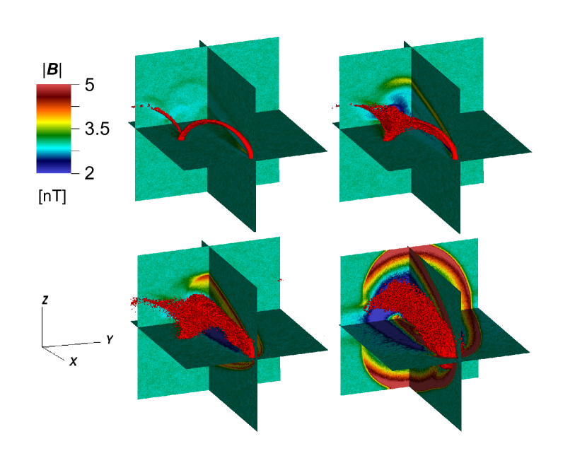
Figure 1: Results for relative heavy ion production of 0.01 (top left), 0.1 (top right), 1 (bottom left), and 10 (bottom right). Iso surface of heavy ion number density of 0.01 cm^-3 is shown in red. The colors of the cuts show magnetic field strength according to the color bar. The simulation domain extends to 50 $R_{M}$ down stream of Mars, and the solution is at $t=1200$ s. The cut perpendicular to the $x$-axis is at $x=-1.6\cdot 10^{8}$ m.

For the magnetic field, we can see in Figure 1 that for the lowest production of 0.01 no significant bow shock is formed, there are however field disturbances associated with the picked-up ions. For larger production a bow shock is formed that strengthen with increased production. We also see that the outflowing ions generate field disturbances downstream that resembles a break in the bow shock,

For the production 1 case we show in Figure 2 the total O⁺ number flux as a function of distance downstream of Mars, for different simulation times. We see that the simulation reaches a steady state situation after 900 seconds.

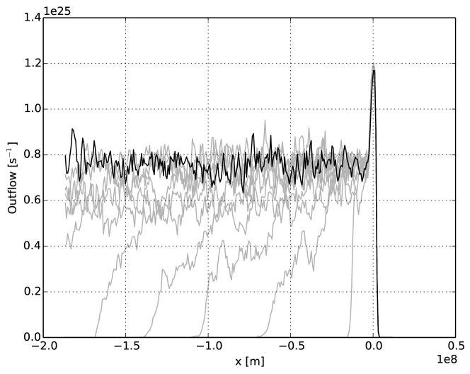
Figure 2: Total O⁺ number flux through planes perpendicular to the $x$-axis for a relative heavy ion production of 1, at different times. The black line is at the final time of 1100 s, and the grey lines are at earlier times in intervals of 100 s.

In Figure 3 we show the average velocity of O⁺ ions as a function of distance downstream of Mars. It takes 45 Mars radii before the heavy ions reach the solar wind velocity of 400 km/s. Visible is also the gyration of some of the ions, as a drop in velocity at about -30 $R_{M}$. This is due to the cycloid motion of the picked-up heavy ions.

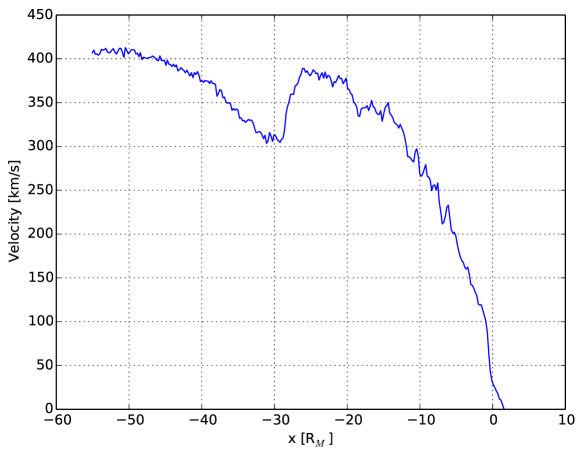
Figure 3: The average velocity of O⁺ ions in planes perpendicular to the $x$-axis for a relative heavy ion production of 1, after 1100 seconds. The velocity is computed as the total ion current divided by total charge in each plane.

We now examine how the outflow changes with production. In Table 1 we show the total outflow of O⁺ ions for different normalized production values. We do not include the outflow for a production of 10 since that simulation did not reach a steady state after 1200 s. The heavy ions accumulated over time close to the planet and were not transported away to escape. The outflow is determined as an average behind Mars at a time of steady state, as shown in Figure 2 for the case when the production is 1.

Table 1: Total outflow of O⁺ ions as a function of normalized production.

Production	0.01	0.1	1
Outflow [s-1]	2.8$\cdot 10^{23}$	2.6$\cdot 10^{24}$	0.7$\cdot 10^{25}$

We see in Table 1 that the outflow increases linear with the production for low productions (from 0.01 to 0.1). For higher productions (from 0.1 to 1) the outflow levels off.

In Fig. 4 we show the magnetic field strength and the heavy ions for a run out to 100 $R_{M}$ downstream of Mars. On this large scale, we clearly see the mix of two different populations of escaping O⁺. One population is the picked-up O⁺ that is visible to the left, moving in cycloid motion perpendicular to the IMF. The other population is a more fluid-like bulk flow of heavy ions going down stream in the $-x$-direction. We also see how the Mach cone is disturbed and penetrated by the escaping heavy ions. The bulk flow is several $R_{M}$ above the plane of the IMF, and is not extended much even at this far distance from the planet. There is some spreading in the plane of the IMF (the $xy$-plane), but not much in the direction perpendicular to the IMF plane.

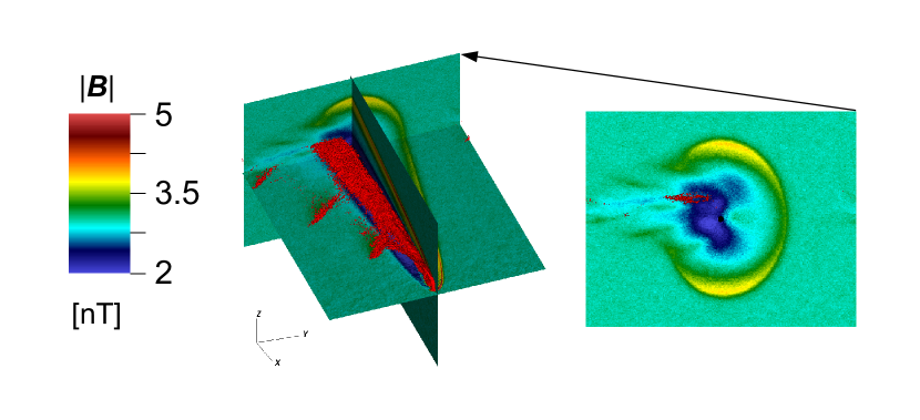
Figure 4: Results for a relative heavy ion production of 1. Iso surface of heavy ion number density of 0.02 cm^-3 is shown in red. The colors of the cuts show magnetic field strength according to the color bar. The simulation domain extends to 100 $R_{M}$ down stream of Mars, and the solution is at $t=1200$ s. The cut perpendicular to the $x$-axis is at $x=-3.4\cdot 10^{8}$ m, and the black disk at the center is the projection of Mars onto this plane.

For the simulation out to 100 $R_{M}$ downstream of Mars, we also show the magnetic field magnitude and the proton number density in Fig. 5.

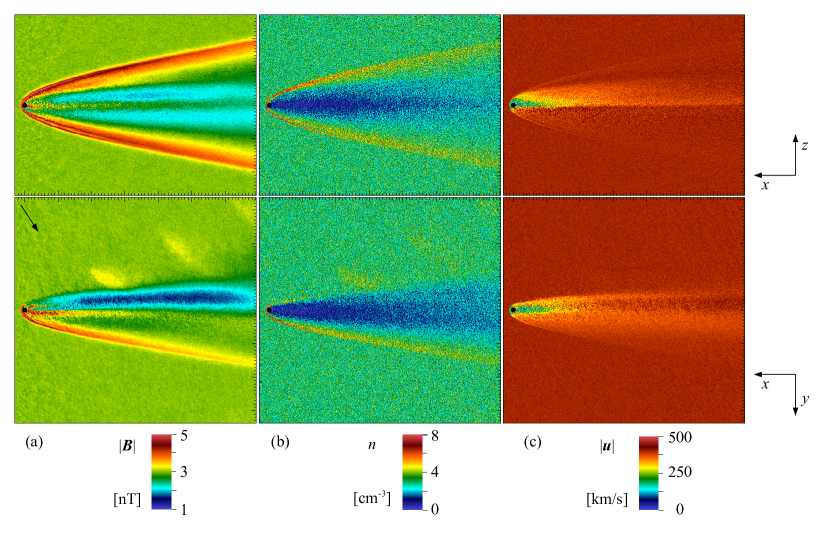
Figure 5: Magnetic field magnitude (a), H⁺ number density (b), and H⁺ velocity magnitude (c), for a relative heavy ion production of 1. Cuts in the $xz$-plane (top) and in the $xy$-plane (bottom). The direction of the interplanetary magnetic field (IMF) in the $xy$-plane is indicated by a black arrow. The simulation domain extends to 100 $R_{M}$ down stream of Mars, and the solution is at $t=1200$ s. The black disk is the projection of Mars. The maximum magnetic field magnitude is 9.3 nT and the maximum number density is 15 cm^-3.

On this scale the bow shock is non-existent in the plane of the IMF on the side where the bow shock normal would be quasi parallel to the IMF. There are however disturbances associated with the gyrating heavy ions. We can also see that the bow shock is split on the quasi perpendicular side, as has been observed closer to Mars in earlier simulations (Modolo et al., 2005). This is seen also in the proton number density, along with also disturbances associated with the gyrating heavy ions. The protons are slowed down close to the planet and in the wake, but are accelerated to solar wind speeds further down stream.

4 Conclusions

We have studied the interaction of Mars with the solar wind on a large scale, out to 100 Mars radii downstream of the planet. A simplified ionosphere as a source of O⁺ ions was used, since details of the ionosphere should not be important on these scales. It was found that on this large scale it is easy to see that the heavy ions escape along two different channels, the proportion depending on the production of heavy ions. For small production the heavies escape mostly as pick-up ions, while for large production the heavies escape as a bulk flow. The ions undergoing pick-up type escape will gyrate around the IMF and leave imprints in the magnetic field and proton densities. The ions subject to a fluid like escape will flow downstream the wake behind Mars without much spreading even at these far distances.

The outflow increases linearly with production up to levels of observed outflow rates, then the escape levels off for higher production rates. It is an open question if there is a maximum escape rate.

The pick-up process will also separate ions with different mass per charge. Here we have only studied O⁺, but the main Martian ionospheric species O⁺, O${}_{2}^{+}$, and CO${}_{2}^{+}$ will all follow different trajectories. This would lead to three different cycloid escape channels.

We found that the solar wind is disturbed by Mars out to 100 $R_{M}$ downstream of the planet, and beyond. We can note that, as seen from Earth, 100 $R_{M}$ is of similar size as the full moon.

References

- Lundin et al. (1989) R. Lundin et al. First results of the ionospheric plasma escape from Mars. Nature, 341:609–612, 1989.
- Lundin et al. (2004) R. Lundin et al. Solar wind-induced atmospheric erosion at Mars: First results from ASPERA-3 on Mars Express. Science, 305:1933–1936, 2004.
- Szegö et al. (2000) Karoly Szegö et al. Physics of mass loaded plasmas. Space Science Reviews, 94(3–4):429–671, 2000. doi: 10.1023/A:1026568530975.
- Kallio and Luhmann (1997) E. Kallio and J.G. Luhmann. Charge exchange near Mars: The solar wind absorption and energetic neutral atom production. Journal of Geophysical Research, 102(A10):22183–22197, 1997.
- Fang et al. (2008) Xiaohua Fang et al. Pickup oxygen ion velocity space and spatial distribution around Mrs. Journal of Geophysical Research, 113:A02210, 2008.
- Ma et al. (2004) Yingjuan Ma et al. Three-dimensional, multispecies, high spatial resolution MHD studies of the solar wind interaction with Mars. Journal of Geophysical Research, 109:A07211, 2004.
- Harnett and Winglee (2006) E. M. Harnett and R. M. Winglee. Three-dimensional multi-fluid simulations of ionospheric loss at Mars from nominal solar wind conditions to magnetic cloud events. Journal of Geophysical Research, 111(A9):A09213, 2006.
- Brecht (1990) Stephen H. Brecht. Magnetic asymmetries of unmagnetized planets. Geophysical Research Letters, 17(9):1243–1246, 1990.
- Kallio and Janhunen (2001) Esa Kallio and Pekka Janhunen. Atmospheric effects of proton precipitation in the Martian atmosphere and its connection to the Mars-solar wind interaction. Journal of Geophysical Research, 106(A4):5617–5634, 2001.
- Modolo et al. (2005) R. Modolo et al. Influence of the solar EUV flux on the Martian plasma environment. Annales Geophysicae, 23:433–444, 2005.
- Bößwetter et al. (2007) A. Bößwetter et al. Comparison of plasma data from ASPERA-3/Mars-Express with a 3-D hybrid simulation. Annales Geophysicae, 25:1851–1864, 2007.
- Brain et al. (2010) D. Brain et al. A comparison of global models for the solar wind interaction with Mars. Icarus, 206:139–151, 2010.
- Brecht and Ledvina (2012) Stephen H. Brecht and Stephen A. Ledvina. Control of ion loss from mars during solar minimum. Earth Planets Space, 64, 165–178, 2012, (64):165––178, 2012.
- Liemohn et al. (2014) Michael W. Liemohn, Blake C. Johnson, Markus Fränz, and Stas Barabash. Mars Express observations of high altitude planetary ion beams and their relation to the “energetic plume” loss channel. Journal of Geophysical Research, 119:9702–9713, 2014.
- Curry et al. (2013) S. M. Curry et al. The influence of production mechanisms on pick-up ion loss at Mars. Journal of Geophysical Research, 118:554–569, 2013.
- Holmström et al. (2012) M. Holmström, S. Fatemi, Y. Futaana, and H. Nilsson. The interaction between the moon and the solar wind. Earth, Planets and Space, 64:237–245, 2012. doi: 10.5047/eps.2011.06.040.
- Lindkvist et al. (2015) Jesper Lindkvist, Mats Holmström, Krishan K. Khurana, Shahab Fatemi, and Stas Barabash. Callisto plasma interactions: Hybrid modeling including induction by a subsurface ocean. Journal of Geophysical Research: Space Physics, 120:4877–4889, 2015.
- Holmström (2011) M. Holmström. Hybrid modeling of plasmas. In Proceedings of ENUMATH 2009, the 8th European Conference on Numerical Mathematics and Advanced Applications, pages 451–458. Springer, 2011. ArXiv:0911.4435.
- Holmstrom (2011) M. Holmstrom. An energy conserving parallel hybrid plasma solver. In Proceedings of ASTRONUM-2010, volume 444 of ASP Conference Series, pages 211–216, 2011. arXiv:1010.3291.
- Holmstrom (2013) M. Holmstrom. Handling vacuum regions in a hybrid plasma solver. In Proceedings of ASTRONUM-2012, volume 474 of ASP Conference Series, pages 202–207, 2013. arXiv:1301.0272.
- Kivelson and Russell (1995) Margret G. Kivelson and Christopher T. Russell, editors. Introduction to Space Physics. Cambridge, 1995. Page 187.
- Ramstad et al. (2013) Robin Ramstad et al. Phobos 2/ASPERA data revisited: Planetary ion escape rate from Mars near the 1989 solar maximum. Geophysical Research Letters, 40(3):477–481, 2013.