Effective field theory for nuclear vibrations with quantified uncertainties

Abstract

We develop an effective field theory (EFT) for nuclear vibrations. The key ingredients – quadrupole degrees of freedom, rotational invariance, and a breakdown scale around the three-phonon level – are taken from data. The EFT is developed for spectra and electromagnetic moments and transitions. We employ tools from Bayesian statistics for the quantification of theoretical uncertainties. The EFT consistently describes spectra and electromagnetic transitions for ⁶²Ni, ^98,100Ru, ^106,108Pd, ^110,112,114Cd, and ^118,120,122Te within the theoretical uncertainties. This suggests that these nuclei can be viewed as anharmonic vibrators.

I Introduction

The quest for quadrupole vibrations in atomic nuclei is a long, confusing, and opressing one. Based on the ground-breaking work by Bohr and Mottelson Bohr (1952); Bohr and Mottelson (1953, 1975), low-energy excitations of atomic nuclei are viewed as quadrupole oscillations of the liquid-drop surface. This approach suggests that some spherical nuclei can be viewed as harmonic quadrupole oscillators, i.e. the five-dimensional $U(5)$ symmetric harmonic oscillator determines their spectra and low-lying transitions. Cadmium isotopes, for instance, have been employed as textbook cases of vibrational motion Bohr and Mottelson (1975); Kern et al. (1995); Rowe and Wood (2010). While corresponding harmonic spectra (including one-, two-, and possibly three-phonon states) were early identified in several nuclei, $B(E2)$ transition strengths exhibit considerable deviations from the predictions of the harmonic quadrupole oscillator, see, e.g. Refs. Lehmann et al. (1996); Corminboeuf et al. (2000); Kadi et al. (2003); Yates (2005); Williams et al. (2006); Garrett et al. (2007); Bandyopadhyay et al. (2007); Garrett et al. (2008); Batchelder et al. (2009); Chakraborty et al. (2011); Radeck et al. (2012); Batchelder et al. (2012) for recent references to a long-standing problem de Boer et al. (1965); Bohr and Mottelson (1975). Proposed anharmonicities were deemed insufficient to account for the considerable differences between data and the harmonic model Bès and Dussel (1969); Bohr and Mottelson (1975). Particularly concerning were the considerable variance between $B(E2)$ strengths for decays from two-phonon states (predicted to be equal), and the relatively large diagonal quadrupole matrix elements of low-lying $2^{+}$ and $4^{+}$ states (predicted to vanish), see, e.g. Refs. Garrett and Wood (2010); Yates (2012); Garrett et al. (2012). The observed deviations from the harmonic quadrupole oscillator are sometimes attributed to deformation of these thought-to-be spherical nuclei.

Based on the data it is clear that harmonic quadrupole vibrations have not (yet) been observed in atomic nuclei. It is not clear, however, how to understand the vibrational spectra that are evident in many nuclei. In this paper, we revisit nuclear vibrations within an effective field theory (EFT). The key ingredients of the EFT – quadrupole degrees of freedom, spherical symmetry, the separation of scale between low-lying collective excitations and a breakdown scale at about the three-phonon level – are consistent with data for spins and parities of low-lying states in the nuclei we wish to describe. The low-energy scale is approximately $\omega\approx 0.6$ MeV in nuclei of mass number 100, while the breakdown scale $\Lambda\approx 3\omega$ is due to pairing effects and other excluded physics. At leading order (LO), the EFT yields the harmonic quadrupole oscillator. The breakdown scale is based on the observed proliferation of states at about the three-phonon level, which is clearly incompatible with the expectations from the LO Hamiltonian. In an EFT, corrections to the LO Hamiltonian are due to the excluded physics beyond the breakdown scale. A power counting can be used to estimate their size, and to systematically improve the Hamiltonian – order by order – as well as transition operators. This is the program we follow in this paper.

We note that EFTs now have a decades-old history in the physics of nuclei. Most effort has been dedicated to an EFT of the interactions between nucleons itself, see Refs. Kolck (1999); Bedaque and van Kolck (2002); Epelbaum et al. (2009); Machleidt and Entem (2011) for reviews. Paired with ab initio calculations Navrátil et al. (2009); Barrett et al. (2013); Hagen et al. (2014), such interactions now provide us with a model-independent approach to atomic nuclei. Halo EFT exploits the separation of scale between weakly-bound halo nucleons and core excitations at much higher energy Bertulani et al. (2002); Higa et al. (2008); Hammer and Phillips (2011); Ryberg et al. (2014). The EFT for heavy deformed nuclei Papenbrock (2011); Coello Pérez and Papenbrock (2015) exploits the separation of scale between low-lying rotational modes and higher-energetic vibrations that result from the quantization of Nambu-Goldstone modes in finite systems Papenbrock and Weidenmüller (2014, 2015).

In this paper we also spend a considerable effort on the quantification of theoretical uncertainties. If a theoretical result is within the experimental uncertainties, theorists usually claim success. However, for meaningful predictions, theoretical uncertainties are crucial. Likewise, disagreement between theoretical results and data can only be claimed based on the absence of overlap between theoretical and experimental uncertainties. Thus, the claim that traditional vibrational models do not describe the existing data is hard to quantify in the absence of theoretical uncertainties. This makes uncertainty quantification particularly relevant for this work.

When it comes to theoretical uncertainties, EFTs have a key advantage over models. The power counting immediately provides the EFT practitioner with uncertainty estimates. Very recently, progress has also been made toward the quantification of uncertainties Cacciari and Houdeau (2011); Bagnaschi et al. (2015); Furnstahl et al. (2015a, b) using Bayesian statistics. In an EFT, uncertainties can be quantified because the (testable) expectation of “naturalness” can be encoded into priors. Here, one assumes that natural-sized coefficients govern the EFT expansion for observables. In this work, we build on these advances and also present analytical formulas for uncertainty quantification based on log-normal priors that are so relevant for EFTs.

This paper is organized as follows. In Sect. II, we develop the EFT for nuclear vibrations and construct the Hamiltonian and electromagnetic operators. In Sect. III we employ Bayesian tools for uncertainty quantification based on the the assumption of natural sized coefficients in the EFT expansion for observables. We compare theoretical results with data for spectra and for electromagnetic moments and transitions in Sect. IV and Sect. V, respectively. Finally, we present our summary in Sect. VI. More detailed derivations are relegated to the Appendix A.

II Effective theory for quadrupole vibrators

In this Section, we develop the EFT for nuclear vibrations. As our intended audience is wide, we aim at a self-contained description. In the following subsections we will introduce the leading-order Hamiltonian, discuss the power counting and higher-order corrections, and develop electromagnetic couplings and observables.

II.1 Leading-order Hamiltonian and spectrum

The spins and parities of low-energy spectra of even-even nuclei near shell closures suggest these can be described in terms of quadrupole degrees of freedom. In several cases, the spectrum resembles – at least at low energies – that of a quadrupole harmonic oscillator. In nuclei with mass number about 100, the oscillator spacing is $\omega\approx 0.6$ MeV. The fermionic nature of the nucleus manifests itself through pair-breaking effects wich enter at about 2–3 MeV of excitation Dean and Hjorth-Jensen (2003). Thus the breakdown scale will be $\Lambda\approx 3\omega$, and for definiteness we will set $\Lambda=3\omega$ in this work.

The boson creation and annihilation operators $d_{\mu}^{\dagger}$ and $d_{\mu}$ with $\mu=-2,-1,\ldots,2$, respectively, fulfill the usual commutation relations

$$\left[d^{\dagger}_{\mu},d_{\nu}\right]=-\delta_{\mu}^{\nu}.$$ (1)

We note that $d_{\mu}^{\dagger}$ are the components of the rank-two spherical tensor $d^{\dagger}$. For the general construction of spherical tensors we also introduce the spherical rank-two tensor $\tilde{d}$ with components

$$\tilde{d}_{\mu}=(-1)^{\mu}d_{-\mu}.$$ (2)

For the construction of spherical tensors we follow Ref. Varshalovich et al. (1988) and introduce tensor products and scalar products. The spherical tensor $\mathcal{I}^{(I)}$ of rank $I$

$$\mathcal{I}^{(I)} = \left(\mathcal{M}^{(I_{1})}\otimes\mathcal{N}^{(I_{2})}\right)^{(I)}$$ (3)

results from coupling the spherical tensors $\mathcal{M}^{(I_{1})}$ and $\mathcal{N}^{(I_{2})}$ of ranks $I_{1}$ and $I_{2}$ respectively. Its components

$$\mathcal{I}_{M}^{(I)}=\sum_{M_{1}M_{2}}C_{I_{1}M_{1}I_{2}M_{2}}^{IM}\mathcal{M}_{M_{1}}^{(I_{1})}\mathcal{N}_{M_{2}}^{(I_{2})}$$ (4)

are given in terms of the Clebsch-Gordan coefficients $C_{I_{1}M_{1}I_{2}M_{2}}^{IM}$ that couple spins $I_{1}$ and $I_{2}$ to spin $I$. Similarly, the scalar product of two spherical tensors $\mathcal{M}^{(I)}$ and $\mathcal{N}^{(I)}$ of the same rank $I$ is

$$\mathcal{M}^{(I)}\cdot\mathcal{N}^{(I)} = \sum_{\mu}(-1)^{\mu}\mathcal{M}_{\mu}^{(I)}\mathcal{N}_{-\mu}^{(I)}$$ (5)

$$= \sqrt{2I+1}\left(\mathcal{M}^{(I)}\otimes\mathcal{N}^{(I)}\right)^{(0)}.$$ (6)

There are two simple operators we need to consider. The number operator

$$\hat{N}\equiv d^{\dagger}\cdot\tilde{d}$$ (7)

is a scalar that counts the total number of phonons $N$. The angular momentum operator is the vector

$$\hat{\mathbf{I}}=\sqrt{10}\left(d^{\dagger}\otimes\tilde{d}\right)^{(1)}.$$ (8)

Both operators conserve the number of phonons. We note that the commutator relations

$$\left[\hat{I}_{\mu},d^{\dagger}_{\nu}\right] = \sqrt{6}C_{2\nu 1\mu}^{2\nu+\mu}d^{\dagger}_{\nu+\mu},$$ (9)

$$\left[\hat{I}_{\mu},\tilde{d}_{\nu}\right] = \sqrt{6}C_{2\nu 1\mu}^{2\nu+\mu}\tilde{d}_{\nu+\mu},$$ (10)

clearly identify $d^{\dagger}$ and $\tilde{d}$ as spherical tensors of rank two. In contrast, $d_{\mu}$ are not components of a spherical tensor.

The Hamiltonian must be a scalar under rotation. The simplest (i.e. quadratic in the fields $d^{\dagger}$ and $\tilde{d}$) Hamiltonian is

$$\hat{H}_{\rm LO} = \omega\hat{N}$$ (11)

$$= \omega\sum_{\mu}(-1)^{\mu}d^{\dagger}_{\mu}\tilde{d}_{-\mu}$$

$$= \omega\sum_{\mu}d^{\dagger}_{\mu}d_{\mu}.$$

Here, $\omega$ is a low-energy constant (LEC) that has to be adjusted to data. We note that one could also consider an operator proportional to

$$d^{\dagger}\cdot d^{\dagger}+\tilde{d}\cdot\tilde{d}$$ (12)

as part of the LO Hamiltonian. However, a Bogoliubov transformation that introduces (quasi-)boson creation and annihilation operators

$$D^{\dagger}_{\mu}=u_{\mu}^{*}d^{\dagger}_{\mu}+v_{\mu}^{*}\tilde{d}_{\mu},\qquad D_{\mu}=u_{\mu}d_{\mu}+v_{\mu}\tilde{d}^{\dagger}_{\mu}$$ (13)

with $|u_{\mu}|^{2}-|v_{\mu}|^{2}=1$ would transform such a Hamiltonian into the diagonal form

$$\hat{H}_{\rm LO}=\tilde{\omega}\left(D^{\dagger}\cdot\tilde{D}\right).$$ (14)

Here $\tilde{D}$ is defined in terms of $D$ similar to Eq. (2). This Hamiltonian conserves the number of (quasi-)bosons and can not be distinguished from the LO Hamiltonian (11).

Clearly, the LO Hamiltonian of the EFT for nuclear vibrations is equivalent to the quadrupole vibrator submodel of the Bohr Hamiltonian Bohr (1952); Bohr and Mottelson (1953, 1975); Iachello and Arima (1987); Rowe and Wood (2010). We note that the five-dimensional quadrupole oscillator exhibits an $U(5)$ symmetry. Within the EFT approach, this symmetry is a (trivial) consequence for the choice of degrees of freedom and the quadratic LO Hamiltonian. While this symmetry might be useful in labeling basis states, it does not reflect symmetry properties of the nuclear interaction between nucleons.

The energies of the LO Hamiltonian

$$\hat{H}_{\rm LO}|\psi\rangle=E_{\rm LO}|\psi\rangle$$ (15)

are

$$E_{\rm LO}=\omega N.$$ (16)

For the construction of the eigenstates we follow Rowe and Wood, and also refer the reader to Ref. Caprio et al. (2009). The eigenstates of the LO Hamiltonian can be labeled by the quantum numbers of the symmetry subgroups in the chain

$$\begin{array}[]{ccccccccc}{\rm U(5)}&\supset&{\rm SO(5)}&\supset&{\rm U(3)}&\supset&{\rm SO(3)}&\supset&{\rm SO(2)}\\ N&&v&&\nu&&I&&M\end{array}.$$

Here $\nu$ is a radial quantum number, $I$ and $M$ are the usual SO(3) angular momentum and its projection onto the $z$-axis, while the seniority $v$ is the SO(5) analog of the angular momentum. From now on, we refer to the SO(3) angular momentum as spin.

The ground state of the system is the phonon vacuum, denoted by $|0\rangle$. A state with $N$ excited quanta is created from the vacuum by the application of $N$ creation operators, coupled to appropriate spin. Given the quantum numbers $v$ and $\nu$, the highest-weight state is defined by

$$|N=v+2\nu,v,\nu,I=2v,M=2v\rangle\propto\left(d^{\dagger}\cdot d^{\dagger}\right)^{\nu}\left(d^{\dagger}_{2}\right)^{v}|0\rangle.$$ (17)

Here, the proportionality sign expresses the absence of proper normalization on the right-hand side. The remaining states with $N=v+2\nu$ phonons can be reached from the highest-weight states by the application of suitably defined lowering operators. This construction is similar to the construction of SO(3) irreducible eigenstates where one starts from the state $|I,M=I\rangle$ and obtains the remaining states of the spin-$I$ multiplet by successive application of the spin-lowering operator. For the LO Hamiltonian, one finds a singlet with spin $I=2$ at the one-phonon level, a triplet with spins $I=0,2,4$ at the two-phonon level, and a quintuplet with spins $I=0,2,3,4,6$ at the three-phonon level. It is convenient to determine the LEC $\omega$ from the excitation energy of the one-phonon state.

II.2 Power counting and NLO corrections

Quadrupole excitations are the low-lying collective degrees of freedom in even-even nuclei systems near shell closures. This picture breaks down at higher energies $\Lambda$ when the microscopic structure of the nucleus in terms of underlying fermionic nucleons is resolved.

In an EFT, subleading corrections to the Hamiltonian arise due to the omitted degrees of freedom. As one can write down an unlimited number of rotational scalars in the fields $d^{\dagger}$ and $\tilde{d}$, we need a power counting (in powers of the small parameter $\omega/\Lambda$) for the systematic construction of the EFT, order by order. As the fields $d^{\dagger}$ and $\tilde{d}$ do not carry any dimension, we introduce quadrupole coordinates $\tilde{\alpha}$ and momenta $\pi$ as

$$\tilde{\alpha}_{\mu} \equiv \sqrt{\frac{1}{2}}\ell\left(d^{\dagger}_{\mu}+\tilde{d}_{\mu}\right),$$ (18)

$$\pi_{\mu} = i\sqrt{\frac{1}{2}}\ell^{-1}\left(d^{\dagger}_{\mu}-\tilde{d}_{\mu}\right).$$ (19)

Here $\ell\equiv(B\omega)^{-1/2}$ is the oscillator length, and $B$ is a mass parameter. These degrees of freedom fulfill the canonical commutation relations

$$\left[\pi_{\mu},\alpha_{\nu}\right]=-i\delta_{\mu}^{\nu},\qquad\tilde{\alpha}_{\mu}=(-1)^{\mu}\alpha_{-\mu}.$$ (20)

We note that both $\tilde{\alpha}$ and $\pi$ are spherical tensors of rank two. In terms of them, the LO Hamiltonian can be written as

$$\hat{H}_{\rm LO}=\frac{1}{2B}\left(\pi\cdot\pi+B^{2}\omega^{2}\tilde{\alpha}\cdot\tilde{\alpha}\right)-\frac{5}{2}\omega.$$ (21)

Thus, the size of coordinates and momenta at the $N$-phonon level is

$$\tilde{\alpha}\sim\sqrt{N}\ell\qquad\pi\sim\sqrt{N}\ell^{-1}.$$ (22)

At the breakdown scale, we have by definition

$$B\omega^{2}\tilde{\alpha}^{2}\sim\Lambda,\quad\mbox{and}\quad\frac{\pi^{2}}{B}\sim\Lambda.$$ (23)

Thus,

$$\tilde{\alpha}\sim\sqrt{\frac{\Lambda}{\omega}}\ell,\quad\mbox{and}\quad\pi\sim\sqrt{\frac{\Lambda}{\omega}}\ell^{-1}$$ (24)

at the breakdown scale.

Let us write the subleading corrections to the Hamiltonian (11) as rotationally invariant terms of the form $g_{mn}\pi^{m}\tilde{\alpha}^{n}$, with $m+n>2$. At the breakdown scale $\Lambda$, the energy shift due to these corrections must be so large that $N$-phonon states cannot be distinguished from states with $N\pm 1$ phonons. Thus,

$$g_{mn}\pi^{m}\tilde{\alpha}^{n}\sim\omega,$$ (25)

and this implies

$$g_{mn}\sim\ell^{m-n}\left(\frac{\omega}{\Lambda}\right)^{\frac{m+n}{2}}\omega$$ (26)

for the natural size of these coefficients. When the term $g_{mn}\pi^{m}\tilde{\alpha}^{n}$ is evaluated for coordinates and momenta of size (22), it scales as

$$g_{mn}\pi^{m}\tilde{\alpha}^{n}\sim\varepsilon^{\frac{m+n}{2}}\omega.$$ (27)

Here

$$\varepsilon\equiv(N\omega/\Lambda)$$ (28)

is the relevant dimensionless expansion parameter of our EFT in the $N$-phonon level. We note that leading-order energies scale as $\varepsilon^{0}\omega$.

This simple analysis suggests that terms cubic in the quadrupole fields are the dominant subleading corrections. However, such terms change boson number and thus enter only in second order perturbation theory, yielding a contribution of size $\varepsilon^{3}\omega$. Thus, the next-to-leading order contributions come from those terms quartic in the quadrupole fields that preserve the boson number. They contribute corrections of the size $\varepsilon^{2}\omega$. We note that some collective models differ from the EFT’s power counting by employing cubic terms as dominant subleading corrections, see. e.g. Refs. Bès and Dussel (1969); Gneuss et al. (1969); Gneuss and Greiner (1971); Hess et al. (1980, 1981). We also note that the proliferation of higher-order terms was addressed in some models by only considering certain combinations of operators that are symmetric under exchange of the operators.

We can now also consider the power counting directly for the operators $d^{\dagger}$ and $\tilde{d}$. When acting on states at the breakdown scale $d^{\dagger}\sim\tilde{d}\sim\sqrt{\Lambda/\omega}$. Demanding that a Hamiltonian term of the structure $\omega f_{m}d^{m}$ containing $m$ boson operators is of the size $\omega$ at the breakdown scale thus yields $f_{m}\sim(\omega/\Lambda)^{m/2}$, and the whole term $\omega f_{m}d^{m}$ scales as $\sim\omega(\omega/\Lambda)^{m/2}$ at low energies.

Before we continue, it is interesting to discuss an alternative – and less conservative – understanding of the breakdown scale. One could also assume that the energy corrections of the terms $g_{mn}\pi^{m}\tilde{\alpha}^{n}$ (for $m+n>2$) are of size $\Lambda$ (and not $\omega$) at the breakdown scale. Then, the contributions from such terms scale as $g_{mn}\pi^{m}\tilde{\alpha}^{n}\sim(\omega/\Lambda)^{(m+n)/2}\Lambda$ at low energies. This implies that the off-diagonal terms with $m+n=3$ contribute an energy $\sim\omega^{2}/\Lambda$ in second-order perturbation theory, and this is equal to the contribution of the $m+n=4$ terms in first-order perturbation theory. Such an approach would again differ from the early approach Bès and Dussel (1969) because terms with four boson operators are as important as terms with three boson operators. Compared to the more conservative approach we are taking, this would add two additional terms (namely $(\pi\times\pi)^{(2)}\cdot\tilde{\alpha}$ and $(\tilde{\alpha}\times\tilde{\alpha})^{(2)}\cdot\tilde{\alpha}$) at NLO, increasing the number of unknown LECs considerably. Such an approach would also probably increase the breakdown scale beyond the three-phonon level, making it difficult to identify states at higher energies. Therefore, we did choose a more conservative – and physically better motivated – power counting.

To identify the linearly independent NLO terms that conserve phonon number, we turned to Chapter 3 of Ref. Varshalovich et al. (1988) and determined the following three terms

$$\hat{N}^{2} = \left(d^{\dagger}\cdot\tilde{d}\right)^{2}$$ (29)

$$\hat{\Lambda}^{2} = -\left(d^{\dagger}\cdot d^{\dagger}\right)\left(\tilde{d}\cdot\tilde{d}\right)+\hat{N}^{2}-3\hat{N}$$ (30)

$$\hat{I}^{2} = 10\left(d^{\dagger}\otimes\tilde{d}\right)^{(1)}\cdot\left(d^{\dagger}\otimes\tilde{d}\right)^{(1)}$$ (31)

Here the operator $\hat{\Lambda}$ is the SO(5) analog of the spin $\hat{I}$ (see, e.g., Ref. Rowe and Wood (2010)). The action of these operators on the LO states is

$$\hat{N}^{2}|Nv\nu IM\rangle = N^{2}|Nv\nu IM\rangle$$ (32)

$$\hat{\Lambda}^{2}|Nv\nu IM\rangle = v(v+3)|Nv\nu IM\rangle$$ (33)

$$\hat{I}^{2}|Nv\nu IM\rangle = I(I+1)|Nv\nu IM\rangle.$$ (34)

Thus, at NLO the Hamiltonian takes the form $\hat{H}_{\rm NLO}=\hat{H}_{\rm LO}+\hat{h}_{\rm NLO}$ with

$$\hat{h}_{\rm NLO}=g_{N}\hat{N}^{2}+g_{v}\hat{\Lambda}^{2}+g_{I}\hat{I}^{2}.$$ (35)

Here, the LECs $g_{N}$, $g_{v}$, and $g_{I}$ have to be adjusted to data. The action of the NLO correction (35) on the eigenstates of the LO Hamiltonian yields

$$\hat{h}_{\rm NLO}|Nv\nu IM\rangle=e_{\rm NLO}|Nv\nu IM\rangle$$ (36)

with

$$e_{\rm NLO} = g_{N}N^{2}+g_{v}v(v+3)+g_{I}I(I+1).$$ (37)

The total energy at NLO is thus

$$E_{\rm NLO}=E_{\rm LO}+e_{\rm NLO}$$ (38)

The four LECs $\omega$, $g_{N}$, $g_{v}$, and $g_{I}$ can be determined from the energies of the one-phonon state and the two-phonon states. Higher excited states would then be predictions. It is clear that the quest for higher precision of the EFT, e.g. by including next-to-next-to-leading order terms introduces further LECs and requires even more data to determine the Hamiltonian. This loss of predictive power is unsatisfactory, but it is also clear that an approach solely based on symmetry arguments – as proposed in this work – naturally leads to this state of affairs. We note that the previous approaches Gneuss et al. (1969); Gneuss and Greiner (1971); Hess et al. (1980, 1981) avoid the proliferation of new coupling constants by only considering certain combinations of higher-order terms. From the EFT’s perspective, however, such a selection does not constitute a systematic approach.

The breakdown scale $\Lambda\approx 3\omega$ is not sufficiently large to study contributions beyond NLO. To improve predictive capabilities, we will quantify (rather than estimate) theoretical uncertainties. This is done in Sect. III.

II.3 Electromagnetic couplings

Our EFT deals with quadrupole degrees of freedom. As the gauge potential $\mathbf{A}(\mathbf{r})$ is a vector field, the electromagnetic coupling of the EFT is not obvious. We can view the quadrupole degrees of freedom as components of a scalar field that depends on the position coordinate $\mathbf{r}$. This view suggests to employ $\mathbf{r}=r\mathbf{e}_{r}(\theta,\phi)$ (with $\mathbf{e}_{r}$ being the usual radial unit vector Varshalovich et al. (1988)) and to expand the vector potential as Eisenberg and Greiner (1970)

$$\mathbf{A}(r,\Omega) = \sum_{JM}\sum_{l}A_{JM,l}j_{l}(kr)\sum_{mn}C^{JM}_{lm1n}Y_{lm}(\Omega)\mathbf{e}_{n}\ .$$

Here, we employed spherical basis vectors $\mathbf{e}_{n}$ with $n=0,\pm 1$, and $j_{l}$ denotes the spherical Bessel function. The spherical wave has a momentum $k$. We note that $A_{JM,l}$ are components of a tensor of rank $J$ for fixed $l$.

The quadrupole degrees of freedom of the EFT must couple to the components $A_{2M,l}$, and only $l=1,2,3$ contribute due to triangular relations on spins. In the long wavelength approximation $kr\ll 1$, and $j_{l}(kr)\propto(kr)^{l}$. Thus, $A_{2M,1}$ is the dominant contribution, and we gauge

$$\pi_{\mu}\to\pi_{\mu}-qA_{2\mu,1}\ .$$ (39)

Here, the charge $q$ is a LEC that needs to be adjusted to data. We are interested in single-photon transitions and only consider terms linearly in $\mathbf{A}$. The effective electric quadrupole operator, resulting from gauging the LO Hamiltonian (11), is thus

$$\hat{Q}_{\rm LO} = -{q\over B}\sum_{\mu}(-1)^{\mu}A_{2\,-\mu,1}\pi_{\mu}$$ (40)

$$= -{iq\over\sqrt{2}B\ell}\sum_{\mu}(-1)^{\mu}A_{2\,-\mu,1}\left(d^{\dagger}_{\mu}-\tilde{d}_{\mu}\right).$$

Let us also consider higher-order corrections. Hamiltonian terms involving two momentum operators $\pi_{\mu}$ and one coordinate operator $\tilde{\alpha}_{\mu}$ contribute to the energy at next-to-next-to leading order, and were beyond the NLO corrections discussed in this section. When considering single-photon transitions, gauging essentially replaces one of the two momentum operators by the gauge field and couples the latter to an operator of the structure

$$\left(\pi\times\tilde{\alpha}\right)^{(2)}\propto-i\left(d^{\dagger}\times d^{\dagger}-\tilde{d}\times\tilde{d}\right)^{(2)}\ .$$ (41)

The EFT expectation is that this operator yields a correction of relative size $\varepsilon^{1/2}$ to the LO operator (40). It induces transitions between states that differ by two phonon numbers, and we will come back to this point after discussing non-minimal couplings.

Let us also consider non-minimal couplings and work in the Coulomb gauge. Then, the electric field is $\mathbf{E}=-\partial_{t}\mathbf{A}=-ik\mathbf{A}$. Here, we assumed an exponential time dependence and set the speed of light to $c=1$. We note that $k\approx\omega$ for transitions between states that differ by one phonon number. The electric field has an expansion similar to Eq. (II.3), and the expansion coefficients fulfill $E_{JM,l}=-ikA_{JM,l}$. The electric field couples to the quadrupole operator

$$\hat{Q}_{\mu} = {\sqrt{2}\over\ell}Q_{0}\tilde{\alpha}_{\mu}$$ (42)

$$+ {2\over\ell^{2}}Q_{1}(\tilde{\alpha}\times\tilde{\alpha})^{(2)}_{\mu}$$

$$+ {2\sqrt{2}\over\ell^{3}}\sum_{L=0,2,4}Q_{2L}\left(\tilde{\alpha}\times\left(\tilde{\alpha}\times\tilde{\alpha}\right)^{(L)}\right)^{(2)}_{\mu}$$

$$+ \ldots\ .$$

Here, factors of the oscillator length $\ell$ have been inserted such that the LECs $Q_{0}$, $Q_{1}$, and $Q_{2L}$ have the dimension of a quadruple moment. The factors of $\sqrt{2}$ are inserted for convenience. The expansion of the quadrupole moment should not be a surprise: what is not forbidden by symmetries is allowed in an EFT. We recall that truly “elementary” degrees of freedom couple to electromagnetic gauge fields solely via minimal coupling. The EFT, however, does not deal with “elementary” degrees of freedom. The quadrupole coordinates of the EFT are effective degrees of freedom at low energies. They are composite and describe collective effects of more microscopic “high-energy” degrees of freedom that are not resolved at the low energy scale we are interested in. The non-minimal couplings allow us to incorporate the sub-leading electromagnetic effects of any microscopic degrees of freedom. Based on the EFT power counting, the natural sizes of the LECs $Q_{1}$ and $Q_{2L}$ are

$$Q_{1} \sim \left({\omega\over\Lambda}\right)^{1/2}Q_{0}\ ,$$

$$Q_{2L} \sim {\omega\over\Lambda}Q_{0}\ .$$ (43)

It is useful to rewrite the expansion (42) in terms of creation and annihilation operators. This yields

$$\hat{Q}_{\mu} = Q_{0}\left(d^{\dagger}_{\mu}+\tilde{d}_{\mu}\right)$$ (44)

$$+ Q_{1}\left(d^{\dagger}\times d^{\dagger}+\tilde{d}\times\tilde{d}+2d^{\dagger}\times\tilde{d}\right)^{(2)}_{\mu}$$

$$+ \sum_{L=0,2,4}Q_{2L}\bigg{(}d^{\dagger}\times\left(d^{\dagger}\times d^{\dagger}\right)^{(L)}+\tilde{d}\times\left(\tilde{d}\times\tilde{d}\right)^{(L)}$$

$$+d^{\dagger}\times\left(d^{\dagger}\times\tilde{d}\right)^{(L)}+d^{\dagger}\times\left(\tilde{d}\times\tilde{d}\right)^{(L)}+\ldots\bigg{)}^{(2)}_{\mu}$$

$$+ \ldots\ .$$

Let us consider the right-hand-side of Eq. (44). The first line is the LO term for transitions between states that differ by one phonon number. It is equivalent to the term (40) obtained from gauging. This allows us to identify

$$q=\sqrt{2}Bk\ell Q_{0}.$$ (45)

The second line of Eq. (44) is the LO term for transitions between states that differ by two-phonon numbers, and also determines diagonal quadrupole matrix elements. Thus, diagonal quadrupole matrix elements are expected to be factor $\sqrt{\omega/\Lambda}$ smaller than transition quadrupole moments between states that differ by one phonon number. The expected finite value for diagonal quadrupole matrix elements is a significant departure from vanishing diagonal quadrupole matrix elements obtained for the harmonic quadrupole vibrator. The third line has NLO corrections (LO terms) for quadrupole transitions between states that differ by one (three) phonon numbers. Thus, the expectations from the harmonic quadrupole vibrator that $B(E2)$ transitions from the two-phonon states to the one-phonon state are independent of the initial spin are expected to suffer corrections of relative size $\omega/\Lambda$. We note that all anharmonic corrections vanish in the harmonic limit, i.e. for $\omega/\Lambda\to 0$.

The reduced matrix elements of a tensor operator $\hat{O}$ of rank $\lambda$ between two states $|i\rangle$ and $|f\rangle$ are defined as

$$\langle f||\hat{O}||i\rangle=\frac{\sqrt{2I_{f}+1}}{C_{I_{i}M_{i}\lambda\mu}^{I_{f}M_{f}}}\langle\beta I_{f}M_{f}|\hat{O}_{\mu}|\alpha I_{i}M_{i}\rangle.$$ (46)

Here $\beta$ and $\alpha$ denote quantum numbers irrelevant for the reduced matrix elements. For the transition quadrupole moments we find the well-known LO reduced matrix elements

$$\langle 0_{1}^{+}||\hat{Q}||2_{1}^{+}\rangle_{\rm LO} = Q_{0}\langle 0_{1}^{+}||d||2_{1}^{+}\rangle=\sqrt{5}Q_{0}\ ,$$

$$\langle 2_{1}^{+}||\hat{Q}||0_{2}^{+}\rangle_{\rm LO} = Q_{0}\langle 2_{1}^{+}||d||0_{2}^{+}\rangle=\sqrt{2}Q_{0}\ ,$$

$$\langle 2_{1}^{+}||\hat{Q}||2_{2}^{+}\rangle_{\rm LO} = Q_{0}\langle 2_{1}^{+}||d||2_{2}^{+}\rangle=\sqrt{10}Q_{0}\ ,$$

$$\langle 2_{1}^{+}||\hat{Q}||4_{1}^{+}\rangle_{\rm LO} = Q_{0}\langle 2_{1}^{+}||d||4_{1}^{+}\rangle=\sqrt{18}Q_{0}\ ,$$ (47)

and uncertainty estimates are of order $Q_{0}\omega/\Lambda$.

For transitions between two-phonon states we find

$$\langle 2_{2}^{+}||\hat{Q}||0_{2}^{+}\rangle_{\rm LO} = 2Q_{1}\langle 2_{2}^{+}||\left(d^{\dagger}\times\tilde{d}\right)^{(2)}||0_{2}^{+}\rangle$$

$$= 4Q_{1}\ ,$$

$$\langle 2_{2}^{+}||\hat{Q}||4_{1}^{+}\rangle_{\rm LO} = 2Q_{1}\langle 2_{2}^{+}||\left(d^{\dagger}\times\tilde{d}\right)^{(2)}||4_{1}^{+}\rangle$$ (48)

$$= {24\over 7}Q_{1}\ ,$$

and uncertainty estimates are of order $Q_{1}\omega/\Lambda$.

For the diagonal quadrupole matrix elements we find the LO reduced matrix elements

$$\langle 2_{1}^{+}||\hat{Q}||2_{1}^{+}\rangle_{\rm LO} = 2Q_{1}\langle 2_{1}^{+}||\left(d^{\dagger}\times\tilde{d}\right)^{(2)}||2_{1}^{+}\rangle$$

$$= 2\sqrt{5}Q_{1}\ ,$$

$$\langle 2_{2}^{+}||\hat{Q}||2_{2}^{+}\rangle_{\rm LO} = 2Q_{1}\langle 2_{2}^{+}||\left(d^{\dagger}\times\tilde{d}\right)^{(2)}||2_{2}^{+}\rangle$$

$$= -{{6\sqrt{5}}\over 7}Q_{1}\ ,$$

$$\langle 4_{1}^{+}||\hat{Q}||4_{1}^{+}\rangle_{\rm LO} = 2Q_{1}\langle 4_{1}^{+}||\left(d^{\dagger}\times\tilde{d}\right)^{(2)}||4_{1}^{+}\rangle$$ (49)

$$= {6\sqrt{110}\over 7}Q_{1}\ ,$$

and uncertainty estimates are of order $Q_{1}\omega/\Lambda$. Thus the LEC $Q_{1}$ relates the three diagonal matrix elements (II.3) and the two transition matrix elements (II.3) to each other. This prediction of the EFT will be tested in Sect. V.

For the transition involving a change by two phonons we find

$$\langle 0_{1}^{+}||\hat{Q}||2_{2}^{+}\rangle_{\rm LO} = Q_{1}\langle 0_{1}^{+}||\left(\tilde{d}\times\tilde{d}\right)^{(2)}||2_{2}^{+}\rangle$$ (50)

$$= \sqrt{10}Q_{1}\ ,$$

and uncertainty estimates are of order $Q_{1}\omega/\Lambda$. This non-minimal correction is of the same size as the NLO correction (41) from gauging. The combination of both terms involves the LEC of the term from gauging and the LEC $Q_{1}$. As there is only one $E2$ transition in vibrational nuclei below the breakdown energy (i.e. the three-phonon energy), the EFT has no predictive power for this transition beyond an estimate of its natural size. Therefore, we will not consider it here.

The $B(E2)$ transition strengths are given in terms of the transition matrix elements (II.3) as

$$B(E2,I_{i}\to I_{f})=\frac{|\langle I_{f}||Q||I_{i}\rangle|^{2}}{2I_{i}+1}$$ (51)

We finally also turn to magnetic moments. In the EFT at LO, magnetic moments are due to the vector operator

$$\hat{\mu}=g\hat{I}\ ,$$ (52)

and $g$ is a LEC constant. Thus magnetic moments of states with spin $I$ have the reduced matrix elements

$$\langle I||\hat{\mu}||I\rangle=g\sqrt{I(I+1)(2I+1)}\ .$$ (53)

Corrections from omitted order are of relative size $\varepsilon^{1/2}$ [e.g. from terms such as $(\tilde{\alpha}\times\mu)^{(1)}$]. Thus, LO magnetic moments of $I=4$ states are a factor $\sqrt{6}$ larger than magnetic moments of $I=2$ states. This is another testable prediction of the EFT.

It is interesting to note that anharmonic corrections to the quadrupole operator have been considered early on Bès and Dussel (1969); Bohr and Mottelson (1975). However, Bès and Dussel related the expansion coefficients of the quadrupole operator to those of the Hamiltonian (also using terms cubic in the boson annihilation and creation operators as corrections to the harmonic quadrupole vibrator). While such an approach has fewer adjustable parameters than the EFT we constructed, it did not yield a satisfactory description of ¹¹⁴Cd. Of course, there are no symmetry arguments that would link the expansion coefficients of non-minimal couplings and the Hamiltonian.

Let us briefly recall the adjustable parameters. The EFT for nuclear vibrations employs one LEC at LO [namely $\omega$ in Eq. (16)] and three additional LECs at NLO [namely $g_{N}$, $g_{v}$, and $g_{I}$ in Eq. (37)] for the Hamiltonian. These LECs need to be adjusted to the energies of four states below the three-phonon level. Thus, LO has predictive power while NLO has predictive power only for states at the three-phonon level. As we will see in Sect. IV, NLO predictions for the energy of the $6_{1}^{+}$ state are more accurate than expected.

Below the three-phonon level there are four strong $E2$ transitions ($2_{1}^{+}\to 0_{1}^{+}$, $0_{2}^{+}\to 2_{1}^{+}$, $2_{2}^{+}\to 2_{1}^{+}$, $4_{1}^{+}\to 2_{1}^{+}$) that change phonon number by one unit. They require the LEC $Q_{0}$ to be adjusted to data. The somewhat smaller matrix elements that govern the two $E2$ transitions between the two-phonon states ($4_{1}^{+}\to 2_{2}^{+}$, $2_{2}^{+}\to 0_{2}^{+}$), and the three diagonal $E2$ matrix elements of the states $2_{1}^{+}$, $2_{2}^{+}$, and $4_{1}^{+}$ require the LEC $Q_{1}$ to be adjusted to data. Finally, one LEC [namely $g$ in Eq. (53)] determines the three magnetic moments of the $2_{1}^{+}$, $2_{2}^{+}$, and $4_{1}^{+}$ states. In this way, the EFT provides us with model-independent realtiuons between observables.

III Quantified theoretical uncertainties

The quantification of theoretical uncertainties is of growing interest in nuclear physics. For a wide collection of articles on this topic we refer the reader to the 2015 focus issue and its editorial Ireland and Nazarewicz (2015).

The power counting provides the EFT practitioner with a simple tool to estimate theoretical uncertainties as missing contributions from higher orders. In our case, uncertainties at LO are of the size $\mathcal{O}(\varepsilon^{2}\omega)$ [as they are caused by missing NLO contributions], while uncertainties at NLO are of the size $\mathcal{O}(\varepsilon^{3}\omega)$ [due to contributions beyond NLO]. In such estimates, one implicitly assumes that the dimensionless coefficients in front of these order-of-magnitude estimates are of order one.

To quantify (rather than estimate) theoretical uncertainties requires considerable effort Carlsson et al. (2015); Furnstahl et al. (2015a). In this Section, we follow Refs. Cacciari and Houdeau (2011); Bagnaschi et al. (2015); Furnstahl et al. (2015b) and employ Bayesian statistics for uncertainty quantification. Within this approach, theoretical uncertainties can be expressed as degree-of-belief (DOB) intervals and have a statistical meaning. The construction of such DOB intervals requires one to make detailed quantitative assumptions about the behavior of omitted orders in the power counting. As a result, theoretical predictions and uncertainties can be confronted by data (and underlying assumptions can be verified, or modified if required).

III.1 Analytical results for log-normal priors

In this Subsection we follow Furnstahl et al. and present the formalism required for uncertainty quantification. We also present a few analytical expressions that involve log-normal priors, which are particularly useful when “naturalness” arguments are employed in EFTs.

We are interested in uncertainty estimates for observables computed in an EFT. The power counting, i.e. a small ratio $\varepsilon<1$ [cf. Eq. (28)] of the low-energy scale and the breakdown scale, allows us to expand an observable $X$ as

$$X=X_{0}\sum_{n=0}^{\infty}c_{n}\varepsilon^{n}$$ (54)

Here, $X_{0}$ sets the general scale. In practice, the sum above can only be computed up to and including the term involving $\varepsilon^{k}$. This implies that the relative uncertainty is

$$\Delta_{k}=\sum_{n=k+1}^{\infty}c_{n}\varepsilon^{n}\ .$$ (55)

It is our aim to quantify the uncertainty $\Delta_{k}$. We are particularly interested in quantifying the residual

$$\Delta_{k}^{(M)}=\sum_{n=k+1}^{k+M}c_{n}\varepsilon^{n}\ ,$$ (56)

of the first $M$ missing terms. To quantify uncertainties, one has to make quantitative assumptions about the distribution of the expansion coefficients $c_{n}$. A key assumption is that the expansion coefficients are independent of each other, and assumptions about the distribution of expansion coefficients are employed as priors.

In an EFT, the expansion coefficients are assumed to be of order unity. The log-normal distribution

$${\rm pr}(c)={1\over\sqrt{2\pi}\sigma c}e^{-{1\over 2}\left({\log c\over\sigma}\right)^{2}}$$ (57)

is consistent with this assumption. Choosing for instance $\sigma=\log\alpha$ (with $\alpha>1$), implies that $1/\alpha\leq c\leq\alpha$ with about 68% probability.

The expansion coefficient $c_{n}$ is related to the prior (57) by a second prior ${\rm pr}(c_{n}|c)$. We consider two examples. First, we assume that the log-normal distributed $c$ yields a hard bound on the size of $c_{n}$. Thus,

$${\rm pr}^{(\rm hw)}(c_{n}|c)={1\over 2c}\Theta(c-|c_{n}|)\ .$$ (58)

Here $\Theta(x)$ denotes the unit step function. The priors (57) and (58) are “set B” of Ref. Furnstahl et al. (2015b). Alternatively, we assume that the log-normal distributed $c$ is related to the width of the Gaussian prior

$${\rm pr}^{(\rm G)}(c_{n}|c)={1\over\sqrt{2\pi}c}e^{-{c_{n}^{2}\over 2c^{2}}}\ .$$ (59)

Following Furnstahl et al. (2015b) the application of Bayes’ theorem yields a probability distribution function for the uncertainty $\Delta$, which we write as

$$p_{M}(\Delta|c_{0},\ldots,c_{k})=\frac{\int\limits_{0}^{\infty}{\rm d}c\,\,{\rm pr}(c)p_{M}(\Delta|c)\prod\limits_{m=0}^{k}{\rm pr}(c_{m}|c)}{\int\limits_{0}^{\infty}{\rm d}c\,\,{\rm pr}(c)\prod\limits_{m=0}^{k}{\rm pr}(c_{m}|c)}\ .$$ (60)

Here, the prior ${\rm pr}(c)$ is the known (or expected) pdf and ${\rm pr}(c_{n}|c)$ is the pdf for a specific expansion coefficient $c_{n}$ given $c$. The probability of finding an uncertainty $\Delta$ given the priors for $c$ is

$$p_{M}(\Delta|c)\equiv\left[\prod\limits_{n=k+1}^{k+M}\int\limits_{-\infty}^{\infty}{\rm d}c_{n}\,\,{\rm pr}(c_{n}|c)\right]\delta\left(\Delta-\Delta_{k}^{(M)}\right)\ .$$ (61)

We note that the structure of Eq. (60) is quite intuitive. The numerator captures our understanding of how the uncertainty depends on the expansion coefficients given the pdf ${\rm pr}(c)$, while the denominator is a normalization.

Reference Furnstahl et al. (2015b) presents detailed discussions of $p_{M}(\Delta|c_{0},\ldots,c_{k})$ for several combinations of priors but does not give analytical expressions for the log-normal distributed prior relevant for EFTs. In what follows, we derive analytical results for the the pdf (60) based on the hard-wall prior (58) for $M=1,2$. For the Gaussian prior (59), we reduce the pdf (60) to single integrations for general $M$. We hope that these formulas might be useful also for other applications of Bayesian uncertainty quantification in EFTs.

To make progress in computing the pdf (61), we rewrite the $\delta$ function as a Fourier integral

$$\delta\left(\Delta-\Delta_{k}^{(M)}\right) = {1\over 2\pi}\int\limits_{-\infty}^{\infty}{\rm d}t\,\,e^{it\Delta}\prod\limits_{n=k+1}^{k+M}e^{-itc_{n}\varepsilon^{n}}\ .$$

Thus, $p_{M}(\Delta|c)$ is the Fourier transform of a product of Fourier transforms

$$p_{M}(\Delta|c)=$$ (62)

$${1\over 2\pi}\int\limits_{-\infty}^{\infty}{\rm d}te^{i\Delta t}\prod\limits_{n=k+1}^{k+M}\int\limits_{-\infty}^{\infty}{\rm d}c_{n}{\rm pr}(c_{n}|c)e^{-it\varepsilon^{n}c_{n}}\ .$$

We evaluate the pdf (62) for the Gaussian prior (59) and find

$$p_{M}^{(\rm G)}(\Delta|c)={1\over\sqrt{2\pi}qc}e^{-{\Delta^{2}\over 2q^{2}c^{2}}}\ .$$ (63)

Here

$$q^{2}\equiv\sum_{n=k+1}^{k+M}\varepsilon^{2n}=\varepsilon^{2k+2}{1-\varepsilon^{2M}\over 1-\varepsilon^{2}}$$ (64)

depends on $M$. Putting all together, we are left with a single integration and can write

$$p_{M}^{(\rm G)}(\Delta|c_{0},\ldots,c_{k})=$$ (65)

$${1\over\sqrt{2\pi}q}\frac{\int\limits_{0}^{\infty}{\rm d}x\,\,x^{k+1}e^{-{1\over 2\sigma^{2}}(\log(x))^{2}}e^{-{\gamma^{2}+\Delta^{2}/q^{2}\over 2}x^{2}}}{\int\limits_{0}^{\infty}{\rm d}x\,\,x^{k}e^{-{1\over 2\sigma^{2}}(\log(x))^{2}}e^{-{\gamma^{2}\over 2}x^{2}}}\ .$$

In this formula, the information from the expansion coefficients enters via

$$\gamma^{2}\equiv\sum_{n=0}^{k}c_{n}^{2}\ .$$ (66)

The numerical evaluation of the pdf (65) poses no difficulty for any value of $M$. Formula (65) is one of the main results in this Subsection.

Let us turn to the hard-wall prior (58). For the computation of the Fourier transform of the prior ${\rm pr}^{(\rm hw)}(c_{n}|c)$ we use

$$\int\limits_{-\infty}^{\infty}{\rm d}c_{n}\,\,{\rm pr}^{(\rm hw)}(c_{n}|c)e^{-itc_{n}\varepsilon^{n}}={\sin{(c\varepsilon^{n}t)}\over c\varepsilon^{n}t}\ ,$$ (67)

and obtain the pdf for the uncertainty $\Delta$ as

$$p_{M}^{(\rm hw)}(\Delta|c)={1\over 2\pi}\int\limits_{-\infty}^{\infty}{\rm d}t\,\,\cos{(t\Delta)}\prod\limits_{n=k+1}^{k+M}{\sin{(c\varepsilon^{n}t)}\over c\varepsilon^{n}t}\ .$$ (68)

As we will see, the integration over ${\rm d}t$ can be performed but becomes cumbersome for $M>1$. Here, we focus on $M=1$ and present the result for $M=2$ in the App. A. For $M>2$ it might be attractive to perform the integrations numerically. In this case, two integrations [one over ${\rm d}t$ for $p_{M}(\Delta|c)$ and one over ${\rm d}c$] remain for the computation of Eq. (60), and this number is independent of $M$.

We set $M=1$ in Eq. (68) and obtain Gradshteyn and Ryzhik (2014)

$$p_{1}^{(\rm hw)}(\Delta|c)={1\over 2c\varepsilon^{k+1}}\Theta\left(c\varepsilon^{k+1}-|\Delta|\right)\ .$$ (69)

This result can also be written as $p_{1}^{(\rm hw)}(\Delta|c)={\rm pr}^{(\rm hw)}(\Delta|c)/(c\varepsilon^{k+1})$. It could also have been obtained by direct evaluation of the ${\rm d}c_{k+1}$ integration in Eq. (60) exploiting the $\delta$ function.

Let us compute $p_{1}^{(\rm hw)}(\Delta|c_{0},\ldots,c_{k})$. We insert the pdf (69) and the priors (57) and (58) into Eq. (60), and perform the integrations (see App. A for details). This yields

$$p_{1}^{(\rm hw)}(\Delta|c_{0},\ldots,c_{k})={e^{{2k+3\over 2}\sigma^{2}}\over 2\varepsilon^{k+1}}\frac{1-\Phi\left({\sigma\over\sqrt{2}}\left(k+2+{\log b\over\sigma^{2}}\right)\right)}{1-\Phi\left({\sigma\over\sqrt{2}}\left(k+1+{\log a\over\sigma^{2}}\right)\right)}\ ,$$ (70)

Here, $\Phi(x)\equiv(2/\sqrt{\pi})\int_{0}^{x}{\rm d}t\exp{(-t^{2})}$ denotes the error function,

$$a\equiv\max(|c_{0}|,\ldots,|c_{k}|),$$ (71)

and

$$b\equiv\max\left(a,{|\Delta|\over\varepsilon^{k+1}}\right).$$ (72)

Let us discuss the result (70). Increasing $\Delta$ from zero, $p_{1}^{(\rm hw)}(\Delta|c_{0},\ldots,c_{k})$ remains a constant for $b\leq a$, i.e. for $\Delta\leq a\varepsilon^{k+1}$. Past this point, $p_{1}^{(\rm hw)}(\Delta|c_{0},\ldots,c_{k})$ decays rapidly to zero as $1-\Phi$ approaches zero for increasing values of its argument.

For $k\gg 1$, we have

$$1-\Phi(x)\approx{e^{-x^{2}}\over\sqrt{\pi}x}\ ,$$ (73)

and obtain for $b\leq a$

$$p_{1}^{(\rm hw)}(\Delta|c_{0},\ldots,c_{k})\approx{1\over 2a\varepsilon^{k+1}}\ .$$ (74)

Interestingly, the same value is found if the priors (57) and (58) are replaced by “set A” of Ref. Furnstahl et al. (2015b). This sheds light on the recent observation Furnstahl et al. (2015b) that DOB percentages depend very mildly on the prior as $k$ increases.

So far, we have limited our considerations to priors ${\rm pr}(c_{n}|c)$ that have zero mean $\overline{c_{n}}=0$. If one drives an EFT to sufficiently high order, one could actually study the distribution of the expansion coefficients $c_{n}$ and thereby assess the prior. As we will see below, priors of interest to our applications have a nonzero mean $\overline{c_{n}}\equiv\langle c_{n}\rangle\neq 0$. Thus, we need to include this information.

In what follows, we assume that the priors for $c_{n}$ with $n\leq k$ have a nonzero mean $\overline{c_{n}}$, but keep the priors for $c_{k+1},c_{k+2},\ldots$, with a zero mean (due to lack of better knowledge). Then

$$p_{M}(\Delta|c_{0},\ldots,c_{k})\to p_{M}\left(\Delta|c_{0}-\overline{c_{0}},\ldots,c_{k}-\overline{c_{k}}\right)\ ,$$ (75)

i.e. one only subtracts the mean from the coefficients $c_{n}$ with $n\leq k$ before inserting them into the analytical formulas.

For the Gaussian prior (59) we would also consider the modification that the log-normal distributed $c$ is proportional (but not equal to) the width of the Gaussian. Thus, we introduce a scale factor $s$ and consider the prior

$${\rm pr}^{(\rm G)}(c_{n}|c)={1\over\sqrt{2\pi}sc}e^{-\left({c_{n}\over 2sc}\right)^{2}}\ .$$ (76)

In this case, we need to replace $q\to sq$ in Eqs. (63) and (65).

Given an interval $[a,b]$ in the domain of a pdf $p(x)$, its degree of belief (DOB) is defined as

$${\rm DOB}(a,b)=\int\limits_{a}^{b}dx\,p(x).$$ (77)

We note that ${\rm DOB}(a,b)\leq 1$, and the DOB of an interval represents the probability for the variable $x$ to take a value within the interval $[a,b]$.

Our probability distributions $p_{M}(\Delta|c_{0},\ldots,c_{k})$ are symmetric around $\Delta=0$. We define the corresponding DOB as

$${\rm DOB}(-\delta,\delta)=\int\limits_{-\delta}^{\delta}{\rm d}x\,p_{M}\left(x|c_{0},\ldots,c_{k}\right).$$ (78)

For a fixed DOB, one can thus give the corresponding uncertainty interval $\pm\delta$. In what follows, we will consider ${\rm DOB}=0.68$. We note that the interval $\pm\delta$ would correspond to the usual one-sigma uncertainty for Gaussian distributions $p_{M}(\Delta|c_{0},\ldots,c_{k})$. Our probability distributions (65) and (70) are, however, not Gaussians.

III.2 Uncertainty quantification for energy levels

Uncertainty quantification is a two-step procedure. First we adjust LECs to data. Second, we quantify uncertainties based on assumptions about the distributions of LECs.

At LO, the energy spectrum is that of a harmonic quadrupole oscillator, see Eq. (16), and the LEC $\omega$ has to be adjusted to data. For nuclear vibrations in the mass $A\approx 100$ region, $\omega\approx 0.6$ MeV. Thus, the distribution of this LEC is relatively sharp. It is neither log-normal distributed, nor is it without a scale (i.e. log-uniform distributed). In what follows, we fix the LEC $\omega$ for each nucleus by performing a least-square fit of the objective function

$$\chi^{2}_{\rm LO}=\sum_{s}\frac{\left[E_{\rm exp}(s)-E_{\rm LO}(s)\right]^{2}}{\sigma_{\rm exp}^{2}+\sigma_{\rm LO}^{2}}.$$ (79)

Here, the sum is over states $s=2_{1}^{+}$, $0_{2}^{+}$, $2_{2}^{+}$, and $4_{1}^{+}$. In the fit, the theoretical uncertainty is estimated as

$$\sigma_{\rm LO}=\omega\left({E_{\rm LO}(s)\over\Lambda}\right)^{2}\ ,$$ (80)

and the experimental uncertainty is neglected because $\sigma_{\rm exp}\ll\sigma_{\rm LO}$.

At NLO, three new LECs ($g_{N}$, $g_{v}$, and $g_{I}$) enter the determination of the energies, see Eq. (38). Instead of re-adjusting $\omega$ at NLO, we replace it by $\omega\to\omega+g_{\omega}$, keep the value of $\omega$ at what was obtained at LO, and adjust $g_{\omega}$. Thus, we rewrite

$$E_{\rm NLO}=\omega N+g_{\omega}N+g_{N}N^{2}+g_{v}v(v+3)+g_{I}I(I+1).$$ (81)

It is clear that the parameters $g_{N}$, $g_{v}$, $g_{I}$, and $g_{\omega}$ are expected to scale as $\omega^{3}/\Lambda^{2}$. In an EFT, one assumes that $g_{\alpha}\Lambda^{2}/\omega^{3}$ (for $\alpha=N,v,I,\omega$) are of order unity and constrained by log-normal distributions. We adjust these coefficients to data by a minimizing the objective function

$$\chi^{2}_{\rm NLO}=\sum_{s}\frac{\left[E_{\rm exp}(s)-E_{\rm NLO}(s)\right]^{2}}{\sigma_{\rm exp}^{2}+\sigma_{\rm NLO}^{2}}.$$ (82)

Here, the employed states $s$ are as for the LO fit, but the theoretical uncertainty is estimated as

$$\sigma_{\rm NLO}=\omega\left({E_{\rm LO}(s)\over\Lambda}\right)^{3}\ .$$ (83)

Again, the experimental uncertainty is again neglected because $\sigma_{\rm exp}\ll\sigma_{\rm NLO}$. As we adjust four parameters to four data points, the fit is exact.

Let us now turn to the quantification of theoretical uncertainties. We note that simple uncertainty estimates can be based on the naive estimates (80) and (83) at LO and NLO, respectively. For quantified uncertainties we adapt the methods of the previous subsection to the problem at hand.

We start with uncertainty quantification at LO. As discussed above, the distribution for $\omega$ is a Dirac delta function, and LO uncertainties are solely due to assumptions about the distribution of LECs from higher orders. Thus,

$$p_{1}^{({\rm hw})}(\Delta)=\frac{e^{\frac{\sigma^{2}}{2}}}{4\varepsilon^{2}}\left[1-\Phi\left(\frac{\sigma}{\sqrt{2}}\left[1+\frac{\log(\Delta/\varepsilon^{2})}{\sigma^{2}}\right]\right)\right]$$ (84)

for the hard-wall prior (58), and

$$p_{M}^{({\rm G})}(\Delta)=\frac{1}{2\pi\sigma qs}\int\limits_{0}^{\infty}dx\,e^{-\frac{\log^{2}x}{2\sigma^{2}}}e^{-\frac{\Delta^{2}x^{2}}{2q^{2}s^{2}}}$$ (85)

for the Gaussian prior (59). Here $q^{2}\equiv\sum_{m=k+1}^{k+M}\varepsilon^{2m}$ with $k=0$ for uncertainties due to $M$ terms above the LO contribution. In Eq. (84) it is assumed that the uncertainty comes fully from the term proportional to $\varepsilon^{2}$.

We now turn to uncertainty quantification at NLO. Returning to Eq. (81), the NLO energy correction for the state $|N,v,I\rangle$ is $\omega\varepsilon^{2}c_{2}$ with

$$c_{2} \equiv c_{2}(N,v,I)$$ (86)

$$= \frac{g_{\omega}N+g_{N}N^{2}+g_{v}v(v+3)+g_{I}I(I+1)}{\varepsilon^{2}\omega},$$

Table 1 shows the resulting coefficients $c_{2}$ for each state of the nuclei ⁶²Ni, ^98,100Ru, ^106,108Pd, ^110,112,114Cd, and ^118,120,122Te considered in this work. These nuclei exhibit low-energy spectra that resemble a harmonic quadrupole oscillator. All coefficients $c_{2}$ are of order one. Thus, the products $\omega\varepsilon c_{2}$ are of natural size. Also shown are the values of the vibrational scale $\omega$ for each nucleus and the LEC $Q_{0}$ associated with the quadrupole moment, see Sect. 3. We note that these quadrupole moments are an order of magnitude smaller than for rotational nuclei Bohr and Mottelson (1975).

Table 1: Values for the vibrational energy $\omega$ (in keV), the coefficients $c_{2}$ in states up to the two-phonon level, and the LEC $Q_{0}^{2}$ associated with the quadrupole moment (in Weisskopf units) for the nuclei studied in this work.

Nucleus	$\omega$ [keV]	$c_{2}(2_{1}^{+})$	$c_{2}(0_{2}^{+})$	$c_{2}(2_{2}^{+})$	$c_{2}(4_{1}^{+})$	$Q_{0}^{2}$ [W.U.]
62Ni	1147.9	0.55	-0.29	0.19	0.26	10.6
98Ru	668.1	1.02	0.57	0.88	0.83	27.8
100Ru	573.9	2.35	1.39	2.36	1.79	23.6
106Pd	541.8	1.80	1.38	1.36	1.80	30.4
108Pd	464.5	1.14	1.53	0.90	1.51	36.9
110Cd	696.7	1.57	1.32	1.33	1.56	21.1
112Cd	635.2	1.72	0.82	1.14	1.52	23.2
114Cd	578.3	1.72	0.93	1.23	1.53	21.8
118Te	582.9	0.83	-0.52	0.19	0.40	–
120Te	567.8	0.79	0.32	0.71	0.56	31.0
122Te	593.5	-0.08	0.88	0.48	0.17	40.7

To determine a valid prior for the coefficients $c_{2}$ we turn to the distribution of the coefficients $c_{2}$ for an ensemble consisting of one-phonon and two-phonon states in the nuclei we study. The cumulative distribution is shown in Fig. 1. It is well approximated by a Gaussian prior (59) with parameter $s\approx 0.65$, or by a hard-wall prior (58), once the mean is shifted from zero to $\mu\approx 1$. We note that the cumulative distribution is practically unchanged when $c_{2}$ values from three-phonon states are included in the analysis. We employ $\sigma=\log{(3/2)}$ in the log-normal prior (57).

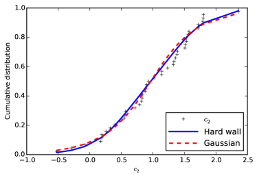
Figure 1: Cumulative distribution for the $c_{2}$ coefficients for states up to the two-phonon level in the ensemble of all nuclei studied in this work. The cumulative distribution of the hard-wall and Gaussian priors is also shown for comparison.

Finally we turn to uncertainty quantification at NLO for individual nuclei. For the hard-wall prior we find

$$p_{1}^{({\rm hw})}\left(\Delta|c_{2}\right)=\frac{e^{\frac{3\sigma^{2}}{2}}}{2\varepsilon^{3}}\frac{1-\Phi\left(\frac{\sigma}{\sqrt{2}}\left[2+\frac{\log(\kappa)}{\sigma^{2}}\right]\right)}{1-\Phi\left(\frac{\sigma}{\sqrt{2}}\left[1+\frac{\log(|c_{2}^{\prime}|)}{\sigma^{2}}\right]\right)}.$$ (87)

Here $\kappa\equiv\max(|c_{2}^{\prime}|,\Delta/\varepsilon^{3})$ and $c_{2}^{\prime}\equiv c_{2}-\overline{c_{2}}$. For the Gaussian prior we find

$$p_{M}^{({\rm G})}\left(\Delta|c_{2}\right)=\frac{\int\limits_{0}^{\infty}dx\,xe^{-\frac{\log^{2}x}{2\sigma^{2}}}e^{-\frac{\left(c_{2}^{\prime 2}+\Delta^{2}/q^{2}\right)x^{2}}{2s^{2}}}}{\sqrt{2\pi}qs\int\limits_{0}^{\infty}dx\,e^{-\frac{\log^{2}x}{2\sigma^{2}}}e^{-\frac{c_{2}^{\prime 2}x^{2}}{2s^{2}}}}.$$ (88)

In the determination of the prior, we employed an ensemble of nuclei. To assess the consistency of this approach, and to verify the statistical interpretation of the quantified uncertainties, we compare EFT predictions for the one-phonon and two-phonon states of these nuclei. To do so, we first normalize the energies by dividing them by the nucleus-dependent $\omega$, and then perform $\chi^{2}$ fits at LO and NLO. The results are shown in Figure 2. Experimental data, LO calculations and NLO calculations are shown as black lines, red crosses and blue diamonds, respectively. The theoretical uncertainty at each order, displayed as a shaded area of the corresponding color, are 68% DOB intervals obtained with the Gaussian prior. We note that 82% of the 44 one- and two-phonon states lie within the NLO theoretical uncertainty. This is within one sigma ($1/\sqrt{44}\approx 15$%) of the expected 68% for the ensemble size. Thus, the statistical interpretation of our DOB intervals is consistent for the energies.

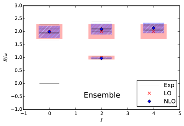
Figure 2: Comparison between the normalized energies $E/\omega$ of the one- and two-phonon states as a function of spin $I$ in the ensemble of the nuclei studied in this work. Experimental energies are shown as thick black lines. 68% DOB intervals are shown as shaded areas (plain for uncertainty quantification at LO and hatched at NLO).

III.3 Uncertainty quantification for quadrupole moments

We quantify uncertainties for LO transition quadrupole moments as follows. The expansion for these matrix elements is

$$\langle f||Q||i\rangle=\langle f||Q||i\rangle_{\rm LO}\left(1+\sum_{i=1}c_{i}\varepsilon^{i}\right),$$ (89)

and coefficients $c_{i}$ that are expected to be of order one. The expansion for the $B(E2)$ transition strength (51) is obtained from the expansion (89) of the corresponding matrix element. We quantify uncertainties for these matrix elements and transition strengths based on Eq. (85) with $s=1$ and compute 68% DOB intervals.

To summarize this Section, we have derived analytical formulas for uncertainty quantifiaction based on log-normal priors. For uncertainty quantification of LO results for energies and matrix elements we employ Eq. (85) with $s=1$ and compute 68% DOB intervals. For uncertainty quantification at NLO for energies, we confirmed that the prior for the employed expansion coefficients is based on data from an ensemble of vibrational nuclei. Based on this ensemble, Eqs. (87) and (88) describe the distribution of uncertainties. These are then used for the computation of 68% DOB intervals.

IV Energy spectra with quantified uncertainties

To test the EFT, we compare the low-energy spectra and reduced transition probabilities of the nuclei ⁶²Ni, ^98,100Ru, ^106,108Pd, ^110,112,114Cd, and ^118,120,122Te against LO and NLO results. We consider nuclei in which the ratio of energies $E(4_{1}^{+})/E(2_{1}^{+})\approx 2$, states with the spins of the two-phonon triplet are at about $2E(2_{1}^{+})$, and states with the spins of the three-phonon quintuplet are around $3E(2_{1}^{+})$. First, we discuss the description of the energy spectra by the EFT. The LECs required for such description were obtained from $\chi^{2}$ fits at LO and NLO, with a breakdown scale set to $\Lambda=3\omega$, based on the appearance of states that cannot be identified with harmonic quadrupole excitations.

The low-lying spectrum of ⁶²Ni exhibits states with the spins and energies of a harmonic quadrupole vibrator up to the three-phonon level, making this nucleus a candidate for low-energy vibrational behavior. The breakdown of vibrational motion at the three-phonon level agrees with the results and discussion for this nucleus presented in Ref. Chakraborty et al. (2011), where shell model calculations with a ⁴⁰Ca core were required to simultaneously describe the energies and electromagnetic properties of some multi-phonon candidates. Similar results for this and other nickel isotopes Kenn et al. (2001); Orce et al. (2008), suggest that intruder configurations need to be taken into account in in a microscopic description of spectra and electromagnetic properties of the low-lying states in these nuclei.

Figure 3 shows the comparison between experimental data taken from Ref. Nichols et al. (2012), LO and NLO calculations for energies up to the three-phonon level for this nucleus. States up to the two-phonon level are shown as thick black lines, while states above them are shown as thin lines whenever a definite spin assignment have been established (consequently, some of the nuclei studied in this work exhibit a higher density of states above the two-phonon level than the one displayed in the figures). The uncertainty at each order is shown as 68% DOB areas. The increased level density above the two-phonon states is consistent with our identification of the breakdown scale at about the three-phonon level. Below the breakdown level, the description of the experimental data is improved order by order. We note that the LO and NLO predictions for three-phonon energies are relatively close.

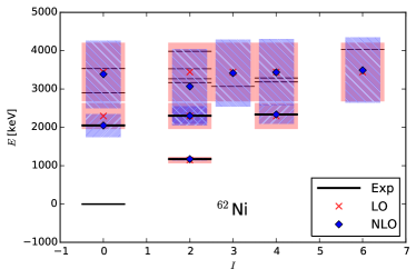
Figure 3: Partial energy spectrum of ⁶²Ni up to the three-phonon level. Experimental data Nichols et al. (2012) is compared to LO and NLO calculations of the effective theory. States up to the two-phonon level are shown as thick black lines. Theoretical uncertainties are shown as 68% DOB intervals.

Let us make three more comments that apply to ⁶²Ni and the other nuclei studied in what follows. First, LO predictions are consistent with data within the quantified theoretical uncertainties. Second, we note that the energies up to the two-phonon states are accurately described at NLO, because the EFT Hamiltonian exhibits four adjustable LECs. Thus, EFT predictions are accurate (they agree with data) yet not very precise (theoretical uncertainties are considerable). The comparison of LO and NLO results shows the convergence properties of the EFT. Third, we also note that the prediction for the $I=6$ three-phonon state is quite accurate. It thus seems that the breakdown scale for yrast states could be higher than for the other states. This is presumably due to the lower level density of high-spin states.

Figure 4 compares the energy spectrum of ⁹⁸Ru (top) and ¹⁰⁰Ru (bottom) and our calculations. Again, the breakdown scale seems properly identified. We note that the differences between LO and NLO predictions for three-phonon levels are considerable.

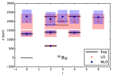
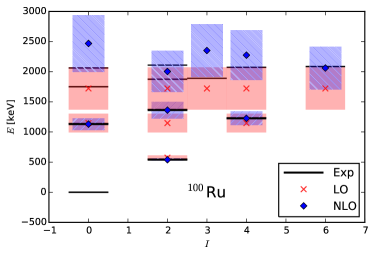
Figure 4: Partial energy spectrum of ⁹⁸Ru (top) and ¹⁰⁰Ru (bottom) up to the three-phonon level. Experimental data Singh and Hu (2003); Singh (2008) is compared to LO and NLO calculations of the effective theory. States up to the two-phonon level are shown as thick black lines. Theoretical uncertainties are shown as 68% DOB intervals.

The ruthenium isotopes near the $N=50$ shell closure appear to undergo a transition from spherical to triaxial shapes, based on the behavior of the ratio $R_{4/2}\equiv E(4_{1}^{+})/E(2_{1}^{+})$ with increasing neutron number Cakirli et al. (2004). From this chain, ⁹⁸Ru is the first isotope expected to exhibit collective behavior based on its ratio of energies $R_{4/2}\approx 2$. Its low-energy spectrum exhibits vibrational-like excitations, with several non-vibrational states above the two-phonon level. Experimental energies were taken from Ref Singh and Hu (2003). For ¹⁰⁰Ru, experimental data were taken from Ref. Singh (2008). Shell model calculations with neutrons promoted across the $N=50$ shell gap reveals the importance of single particle motion in these isotopic chain Kharraja et al. (1999); Timár et al. (2000). As mentioned before, ruthenium isotopes transit from spherical to triaxial shapes as the neutron number increase. Larger deviations from the harmonic behavior in ¹⁰⁰Ru suggest that deviations from the spherical shape are larger than in ⁹⁸Ru.

The energy spectra of ¹⁰⁶Pd and ¹⁰⁸Pd are compared against LO and NLO calculations in the top and bottom of Figure 5 respectively. In ¹⁰⁸Pd there are fewer levels around the three-phonon states. The considerable deviations of the $I=0,2$ three-phonon energies from NLO predictions – consistent with the theoretical uncertainties – nevertheless suggests that the breakdown scale has been identified correctly.

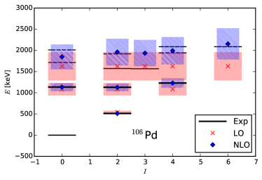
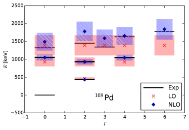
Figure 5: Partial energy spectrum of ¹⁰⁶Pd (top) and ¹⁰⁸Pd (bottom) up to the three-phonon level. Experimental data Frenne and Negret (2008); Blachot (2000) is compared to LO and NLO calculations of the effective theory. States up to the two-phonon level are shown as thick black lines. Theoretical uncertainties are shown as 68% DOB intervals.

The energy spectra and enhanced transitions probabilities for decays from the low-lying states in palladium isotopes, assumed to be spherical, suggest vibrational motion in these systems. For ¹⁰⁶Pd and ¹⁰⁸Pd, experimental data was taken from Ref. Frenne and Negret (2008) and Ref. Blachot (2000) respectively. Single particle states have been suggested for ¹⁰⁸Pd Regan et al. (1997). The palladium isotopes exhibit ratios $R_{4/2}\approx 2.4$ and $B(E2;4_{1}^{+}\downarrow)/B(E2;2_{1}^{+}\downarrow)\approx 1.6$. These quantities, in addition to the large diagonal quadrupole matrix elements for states up to the two-phonon level in palladium isotopes Svensson et al. (1995), strongly suggest that the deviation from the harmonic oscillator behavior in these systems is considerable.

Figure 6 compares experimental spectra of cadmium isotopes with LO and NLO order results from EFT. We note that the deviations from expectations for the harmonic quadrupole vibrator are pronounced in these isotopes, with additional energy levels just above the two-phonon states. We also note that the energies of the three-phonon $6_{1}^{+}$ states deviate stronger from EFT predictions than for the other nuclei we consider in this work. In these nuclei, the breakdown scale for vibrations is clearly low. From the EFTs perspective anharmonic corrections are expected to be most significant.

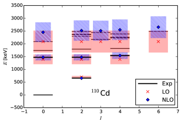
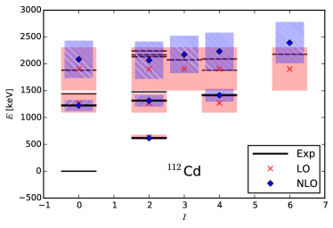
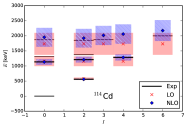
Figure 6: Partial energy spectrum of ¹¹⁰Cd (top), ¹¹²Cd (middle) and ¹¹⁴Cd (bottom) up to the three-phonon level. Experimental data Gurdal and Kondev (2012); Frenne and Jacobs (1996); Blachot (2012) is compared to LO and NLO calculations of the effective theory. States up to the two-phonon level are shown as thick black lines. Theoretical uncertainties are shown as 68% DOB intervals.

The cadmium isotopes have once been considered textbook candidates of low-energy vibrational behavior based only on their energy spectra Bohr and Mottelson (1975); Kern et al. (1995); Rowe and Wood (2010), despite exhibiting intruder states due to protons promoted across the $Z=50$ shell gap around the two-phonon level Heyde et al. (1982); Meyer and Peker (1977). Other studies on cadmium isotopes Corminboeuf et al. (2000); Kadi et al. (2003); Garrett et al. (2007, 2008); Garrett and Wood (2010); Garrett et al. (2012) in which mixing between vibrational and non-vibrational states is taken into account, cannot accurately describe the electromagnetic properties of multi-phonon candidates. They set the breakdown of vibrational behavior at the 3- or two-phonon level depending on the isotope, and suggest a quasi-rotational character for the low-lying excitations, based on the large quadrupole moments of some yrast states Stone (2005); Garrett and Wood (2010). For the three isotopes studied in this work, $A=110,112,114$, experimental data was taken from Refs. Gurdal and Kondev (2012); Frenne and Jacobs (1996); Blachot (2012) respectively. The lowest $0^{+}$ and $2^{+}$ states above the one-phonon level were employed as the two-phonon states for the $\chi^{2}$ fits. The states identified as members of two-phonon triplet in this work might be in disagreement with previous studies Garrett et al. (2007, 2008); Garrett and Wood (2010), where, for example, the $0_{2}^{+}$ in ¹¹²Cd have been identified as an intruder state Heyde et al. (1982); Wood et al. (1992). Here, the identification is made based on the assumption that non-vibrational modes require more energy to be excited. As we discuss in Sect. V, $B(E2)$ values for decays from the identified states seems to be in better agreement with the EFT expectations than those from other states,

Figure 7 shows the comparison between experimental data taken from Refs. Kitao et al. (2002); Tamura (2007) for ¹²⁰ Te and ¹²²Te respectively, and LO and NLO results from EFT.

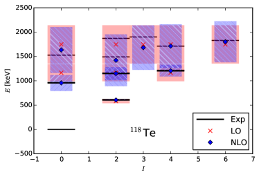
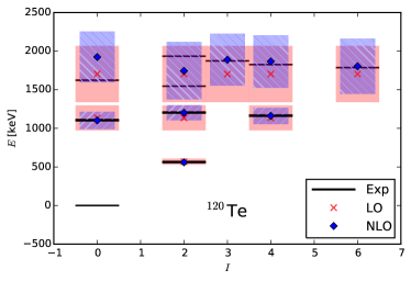
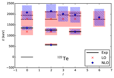
Figure 7: Partial energy spectrum of ¹¹⁸Te, ¹²⁰Te (middle) and ¹²²Te (bottom) up to the three-phonon level. Experimental data Kitao et al. (2002); Tamura (2007) is compared to LO and NLO calculations of the effective theory. States up to the two-phonon level are shown as thick black lines. Theoretical uncertainties are shown as 68% DOB intervals.

The tellurium isotopic chain provide us with some candidates to low-energy vibrational behavior. The isotopes with $A=118,120,122$ all exhibit very similar spectra with states that can be identified with those of a quadrupole vibrator up to the three-phonon level. From these isotopes, the best candidate is ¹²⁰Te with a non-vibrational state slightly above the three-phonon quintuplet. ¹²²Te exhibits a non-vibrational state already at the three-phonon level. The breakdown of the collective behavior is a consequence of competing single-particle motion, know to exist in tellurium isotopes (Paul et al., 1995, 1996; Vanhoy et al., 2003; Hicks et al., 2005, 2008; Nag et al., 2012), and signaled in ¹²²Te by the unusual energy ratios $E(4_{1}^{+})/E(2_{1}^{+})<2$ and $E(6_{1}^{+})/E(4_{1}^{+})<1.5$ Cizewski (1989). The alignment of both valence nucleons and protons promoted across the $Z=50$ shell gap breaks the spherical symmetry and give rise to non-collective deformed states. These states compete energetically with the collective states. In particular, the $6_{1}^{+}$ state have been interpreted both as a vibrational state or in terms of valence protons configurations coupled to a tin core.

Let us summarize our uncertainties as 68% DOB intervals $\pm\delta$ for the hard-wall (hw) prior and the Gaussian (G) prior. The uncertainty is $\omega\delta$ for the energy levels. At LO, the pdfs in Eqs. (84) and (85) agree with each other and yield values of $\delta=0.07$ and $\delta=0.29$ for the one- and two-phonon levels, respectively. At NLO Table 2 summarizes the values of $\delta$ for states up to the two-phonon level. The columns labeled by hw and G show the values of $\delta$ obtained from the pdfs in Eqs. (87) and (88), respectively. With the exception of a few relatively large uncertainties, both priors yield very similar results. For large uncertainties $\delta$, one samples the tails of the respective priors, and these are notably different (and not well constrained by data, cf. Fig. 1).

Table 2: Values of the uncertainties at NLO, with $\pm\delta$ giving the size of 68% DOB intervals in states up to the two-phonon level. The hard-wall (hw) and Gaussian (G) priors we employed the distribution functions (87) and (88), respectively.

	$2_{1}^{+}$		$0_{2}^{+}$		$2_{2}^{+}$		$4_{1}^{+}$
Nucleus	hw	G	hw	G	hw	G	hw	G
62Ni	0.02	0.02	0.29	0.22	0.21	0.20	0.20	0.20
98Ru	0.02	0.02	0.18	0.19	0.18	0.18	0.18	0.18
100Ru	0.04	0.03	0.18	0.18	0.30	0.22	0.21	0.20
106Pd	0.03	0.02	0.18	0.18	0.18	0.18	0.21	0.20
108Pd	0.02	0.02	0.18	0.19	0.18	0.18	0.18	0.19
110Cd	0.02	0.02	0.18	0.18	0.18	0.18	0.19	0.19
112Cd	0.02	0.02	0.18	0.18	0.18	0.18	0.18	0.19
114Cd	0.02	0.02	0.18	0.18	0.18	0.18	0.18	0.19
118Te	0.02	0.02	0.34	0.23	0.21	0.20	0.19	0.19
120Te	0.02	0.02	0.19	0.19	0.18	0.18	0.18	0.19
122Te	0.03	0.03	0.18	0.18	0.18	0.19	0.21	0.20

V Electromagnetic moments – comparison with data

In this Section, we compare our results for transition quadrupole moments, diagonal quadrupole matrix elements, and magnetic moments with data. Theoretical uncertainties are quantified for all quadrupole observables we consider. As we will see, the EFT correctly captures and consistently describes the main experimental features of vibrational nuclei.

To determine the LEC $Q_{0}$ we perform $\chi^{2}$ fits to data at LO with

$$\chi^{2}_{\rm LO}=\sum_{t}\frac{\left[B(E2)_{\rm exp}^{(t)}-B(E2)_{\rm LO}^{(t)}\right]^{2}}{\sigma_{\rm exp}^{2}+\sigma_{\rm LO}^{2}}.$$ (90)

Here $t$ labels the transitions from the one-phonon state to the ground state and from the two-phonon states to the one-phonon state, i.e. $2_{1}^{+}\to 0_{1}^{+}$, $0_{2}^{+}\to 2_{1}^{+}$, $2_{2}^{+}\to 2_{1}^{+}$, and $4_{1}^{+}\to 2_{1}^{+}$. In these fits we estimate the theoretical uncertainty for decays from the $N$-phonon state as

$$\sigma_{\rm LO}=B(E2)_{\rm LO}^{(t)}\varepsilon\ .$$ (91)

Experimental data was mostly taken from the Nuclear Data Sheets for the studied nuclei. For ⁶²Ni, this data was complemented with that from Ref. Chakraborty et al. (2011), while for ⁹⁸Ru we took the data from Ref. Radeck et al. (2012), which establish a ratio $B(E2,4_{1}^{+}\rightarrow 2_{1}^{+})/B(E2,2_{1}^{+}\rightarrow 0_{1}^{+})=1.86(16)$ in agreement with the expectations for vibrators instead of taking data for which this ratio has anomalous values Kharraja et al. (1999); Cakirli et al. (2004); Williams et al. (2006). The lack of experimental data for ¹¹⁸Te makes it impossible to perform $\chi^{2}$ fit. For ¹²⁰Te, we fixed $Q_{0}^{2}$ to the only experimental value, and make predictions for decays from the two-phonon states.

Table 3 compares experimental and theoretical $B(E2)$ values (in Weisskopf units) for each nucleus considered in this work. The theoretical uncertainty is shown as 68% DOB intervals from the pdf (85) with $s=1$. Within the often considerable theoretical uncertainties, the EFT consistently describes the available experimental data. These results, taken together with the results for energy level in Table 2, show that vibrational nuclei can be described as such within an EFT with a breakdown scale around the three-phonon level. They are examples for anharmonic quadrupole oscillators.

Table 3: $B(E2)$ values (in Weisskopf units) for decays from states below the three-phonon level in the ensemble of all studied nuclei. is in agreement with LO calculations below the breakdown level. The theoretical uncertainty is given by the 68% DOB interval for the normalized residual for $B(E2)$ values. States with transition strengths within theoretical uncertainty are characterized as collective vibrations.

Nucleus	$2_{1}^{+}\rightarrow 0_{1}^{+}$	EFT	$0_{2}^{+}\rightarrow 2_{1}^{+}$	$2_{2}^{+}\rightarrow 2_{1}^{+}$	$4_{1}^{+}\rightarrow 2_{1}^{+}$	EFT
62Ni	12.1(4)	11(4)	42(23)	14.9(42)	21(6)	21(7)
98Ru	31(1)	28(9)		47(5)	57.6(40)	56(19)
100Ru	35.6(4)	24(8)	35(5)	30.9(4)	51(4)	47(16)
106Pd	44.3(15)	30(10)	35(8)	44(4)	76(11)	61(20)
108Pd	49.5(13)	37(12)	52(5)	71(5)	73(8)	74(25)
110Cd	27.0(8)	21(7)		30(5)	42(9)	42(14)
112Cd	30.2(3)	23(8)	51(14)	15(3)	61(6)	46(15)
114Cd	31.1(19)	22(7)	27.4(17)	22(6)	62(4)	43(15)
120Te	31 (6)	31(10)				62(21)
122Te	36.9(3)	41(14)		100(30)		81(27)

How reasonable and consistent are the 68% DOB intervals for the $B(E2)$ transitions? To address this question, we turn again to the ensemble of vibrational nuclei considered in this work. Excluding the isotopes ^118,120Te, the EFT prediction $B(E2)/Q_{0}^{2}=N$ for decays from the $N$-phonon state can be compared to the data from all nuclei in the ensemble. This comparison is shown in Fig. 8, where the experimental data and the LO calculations are shown as black errorbars and red lines with shaded uncertainty bands, respectively. About 81% of the data is within the 68% DOB intervals. This is a consistent agreement for an ensemble of 32 data points.

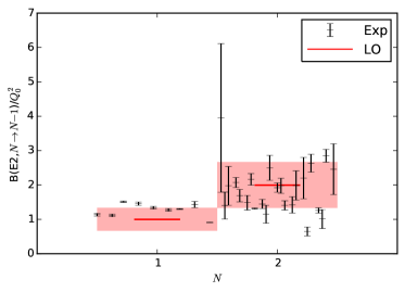
Figure 8: Comparison between the normalized $B(E2)$ values for decays from the one- and two-phonon states in the ensemble of the nuclei studied in this work. Experimental $B(E2)$ values are shown as black lines with error bars. Quantified theoretical uncertainties are shown as shaded areas.

The eigenstates of a harmonic quadrupole oscillator have vanishing diagonal quadrupole matrix elements. Compared to this ideal case, diagonal quadrupole matrix elements for isotopes of Cd and Pd exhibit sizes that are only somewhat smaller than transition quadrupole moments. From the EFT’s perspective, sizeable diagonal quadrupole matrix elements are expected. Comparing the expansion of the spectrum (38) with that of the quadrupole operator (44) shows that anharmonic corrections have relative size $\varepsilon$ for energies and relative size $\varepsilon^{1/2}$ for the quadrupole operator.

Let us consider diagonal quadrupole matrix elements (II.3). We employ experimental data for the diagonal quadrupole matrix elements of the $2_{1}^{+}$, $2_{2}^{+}$ and $4_{1}^{+}$ in ¹⁰⁶Pd and ¹⁰⁸Pd from Svensson et al. and determine the LEC $Q_{1}$ by a $\chi^{2}$ fit to these data. In these fits, the theoretical uncertainty was estimated as $Q_{0}\varepsilon^{3/2}$ as discussed in Subsection II.3.

The fits yield $Q_{1}=-0.14\ e\rm b$ for both palladium isotopes. (We recall that for a nucleus with $A$ nucleons $1~{}\rm{W.~{}U.}=5.94\times 10^{-6}A^{4/3}~{}{\rm e}^{2}\rm{b}^{2}$.) Comparing the size of $Q_{1}$ against $Q_{0}$ yields $Q_{1}/Q_{0}=0.47$ and $Q_{1}/Q_{0}=0.41$ in ¹⁰⁶Pd and ¹⁰⁸Pd, respectively. These ratios are consistent with the EFT estimate $Q_{1}/Q_{0}\sim\varepsilon^{1/2}=\sqrt{1/3}\approx 0.58$. In other words, sizeable diagonal quadrupole matrix elements are not a surprise for these anharmonic vibrators but rather expected and due to the marginal separation of scale, i.e. the breakdown of the EFT around the three-phonon level.

The left part of both panels in Figure 9 compares EFT results to data Svensson et al. (1995) for the diagonal quadrupole matrix elements of the $2_{1}^{+}$, $2_{2}^{+}$ and $4_{1}^{+}$ states in ¹⁰⁶Pd (top) and ¹⁰⁸Pd (bottom). Theoretical uncertainty are shown as 68% DOB bands. They are based on the Gaussian prior (59) and $M=1$ in Eq. (65). Within the theoretical uncertainties, the EFT is consistent with the data.

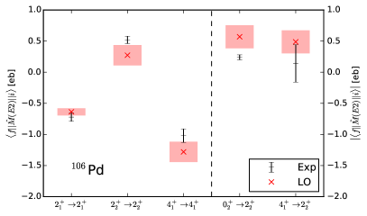
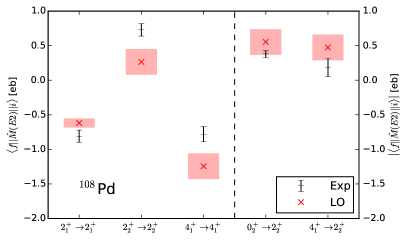
Figure 9: Comparison between data and EFT results for the reduced quadrupole matrix elements for in ¹⁰⁶Pd (top) and ¹⁰⁸Pd (bottom). Experimental data are shown as black lines, while EFT results from LO calculations are shown as red diamonds with uncertainties as shaded 68% DOB intervals. The left part shows diagonal quadrupole matrix elements employed in the fit of the LEC constant $Q_{1}$. The right part shows predictions for the absolute values of the reduced quadrupole matrix elements governing $E2$ transitions between two-phonon states.

We turn to transition quadrupole moments (II.3) between two-phonon states because these are also determined by the LEC $Q_{1}$ and are thus predictions of the EFT. The right part of Fig. 9 shows the magnitude of the transition matrix elements and compares them to data Svensson et al. (1995). We note that the EFT yields different signs of these (non-observable) matrix elements and that only the magnitude of these matrix elements is an observable quantity, see the definition of the observable $B(E2)$ transition strength in Eq. (51).

Theoretical results for quadrupole matrix elements in ¹¹⁴Cd are shown in Fig. 10 and compared to data Fahlander et al. (1988). The uncertainties are quantified as for the palladium isotopes. With the exception of the diagonal matrix element of the $2_{2}^{+}$ state, the EFT yields a consistent description of the data, and has predictive power for the off-diagonal matrix elements. Here, $Q_{0}=0.27$ eb, and $Q_{1}=-0.09$ eb.

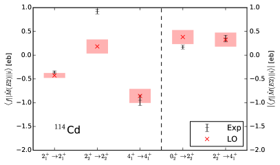
Figure 10: Comparison between data and EFT results for the reduced quadrupole matrix elements for in ¹¹⁴Cd. Experimental data are shown as black lines, while EFT results from LO calculations are shown as red diamonds with uncertainties as shaded 68% DOB intervals. The left part shows diagonal quadrupole matrix elements employed in the fit of the LEC constant $Q_{1}$. The right part shows predictions for the absolute values of the reduced quadrupole matrix elements governing $E2$ transitions between two-phonon states.

Thus, the EFT consistently describes matrix elements of electromagnetic operators. In the present approach, the anharmonicities are due to the operators themselves, with states being the eigenstates of the harmonic quadrupole oscillator. We note that Figs. 9 and 10 exhibit very similar patterns for the different nuclei. As a last consistency check, we turn to magnetic moments.

The EFT needs one magnetic moment to determine an LEC, i.e. the constant $g$ in Eq. (53). While magnetic moments are typically known for the lowest $2^{+}$ state in many even-even nuclei Stone (2005), the EFT can only be tested if more magnetic moments are known below the three-phonon level. The states $2_{1}^{+}$, $2_{2}^{+}$, and $4_{1}^{+}$ have non-zero spins and thus exhibit magnetic moments. As discussed below Eq. (53), the EFT predicts at LO that both $2^{+}$ states have equal magnetic moments, i.e. $\mu(2_{1}^{+})=\mu(2_{2}^{+})\equiv\mu(2^{+})$, and that the $4^{+}$ state has a magnetic moment $\mu(4_{1}^{+})=\sqrt{6}\mu(2^{+})\approx 2.44\mu(2+)$. Weighted averages of the experimental data Stone (2005) [in units of nuclear magnetons (nm)] for ¹⁰⁶Pd shows that $\mu(2_{1}^{+})\approx 0.79\pm 0.02$ nm, $\mu(2_{2}^{+})=0.71\pm 0.10$ nm, and $\mu(4_{1}^{+})=1.8\pm 0.4$ nm. This is consistent with EFT expectations. It would certainly be interesting to test these EFT predictions in other vibrational nuclei.

Overall, the EFTs results and predictions for electromagnetic properties of states and transitions below the three-phonon level are consistent with data. This would make it interesting to measure such complete data sets for other vibrational nuclei as well.

VI Summary

We developed an EFT for collective nuclear vibrations based on quadrupole degrees of freedom, rotational invariance, and a breakdown scale at around the three-phonon level. For spectra, the EFT is driven to next-to-leading order, while the computation of other matrix elments is restricted to leading order. The terms in appearing in the Hamiltonian and quadrupole operator differ from those employed in several models.

The EFT approach also allows us to quantify theoretical uncertainties. To this purpose, we make testable assumptions about priors regarding the distribution of low-energy constants and employ recently developed tools from Bayesian statistics. We give analytical results for the important case of log-normal priors. The priors employed in the uncertainty quantification of energies are consistent for the ensemble of nuclei we considered.

The EFT is minimally coupled to electromagnetic gauge fields in a model-independent way, with non-minimal couplings accounting for subleading corrections. For states below the three-phonon level we describe LO $B(E2)$ transition strengths with quantified uncertainties and present several results for diagonal and off-diagonal matrix elements of the quadrupole operator. Comparing the EFT results to an extensive data set shows that spectra and transition strengths are consistently described within the theoretical and experimental uncertainties for ⁶²Ni, ^98,100Ru, ^106,108Pd, ^110,112,114Cd, and ^118,120,122Te. In particular, relatively large diagonal matrix elements in ^106,108Pd and ¹¹⁴Cd are consistent with the expectations of the EFT. The consistent description of spectra, $E2$ transitions and matrix elements, and magnetic moments within the EFT for nuclear vibration suggests that the nuclei studied in this work can be viewed as anharmonic quadrupole vibrators. This work also suggests that it would be interesting to measure a combination of matrix elements for electric and magnetic observables in nuclei such as ¹²⁰Te and ¹²²Te.

It would be interesting to extend the EFT of nuclear vibrations also to odd-mass neighbors of the even-even nuclei considered in this work. Combining, for instance, halo EFT with this work, one might explore to what extent such nuclei can be understood by coupling the odd nucleon to the quadrupole degrees of freedom of vibrational even-even nuclei.

Appendix A Analytical results for log-normal priors

In this Appendix we present some details for the derivation of analytical results for the combination of log-normal priors (57) and hard-wall priors (58).

The denominator of Eq. (60) is

$$\int\limits_{0}^{\infty}{\rm d}c\,\,{\rm pr}(c)\prod\limits_{m=0}^{k}{\rm pr}^{(\rm hw)}(c_{m}|c)=$$ (92)

$${2^{-(k+1)}\over\sqrt{2\pi}\sigma}\int\limits_{a}^{\infty}{\rm d}c\,\,c^{-(k+2)}e^{-{1\over 2\sigma^{2}}(\log c)^{2}}\ .$$

Here,

$$a\equiv\max(|c_{0}|,\ldots,|c_{k}|)$$ (93)

is a function of the expansion coefficients. Substitutions $z=\log c$ and $x=z-\log(a)$ yield

$$\frac{e^{-(k+1)\log a}e^{-{1\over 2\sigma^{2}}(\log a)^{2}}}{2^{(k+1)}\sqrt{2\pi}\sigma}\int\limits_{0}^{\infty}{\rm d}x\,\,e^{-{x^{2}\over 2\sigma^{2}}-x\left(k+1+{\log a\over\sigma^{2}}\right)}\ .$$ (94)

This integral is known Gradshteyn and Ryzhik (2014), and we find

$$2^{-(k+2)}e^{{\sigma^{2}\over 2}(k+1)^{2}}\left[1-\Phi\left({\sigma\over\sqrt{2}}\left(k+1+{\log a\over\sigma^{2}}\right)\right)\right]$$ (95)

as the final result for the denominator of Eq. (60). Here, $\Phi(x)\equiv(2/\sqrt{\pi})\int_{0}^{x}{\rm d}t\exp{(-t^{2})}$ denotes the error function. The numerator of the expression (60) can be evaluated in similar fashion. Employing the shorthand

$$b\equiv\max\left(a,{|\Delta|\over\varepsilon^{k+1}}\right)$$ (96)

we find for the numerator of Eq. (60)

$${e^{{\sigma^{2}\over 2}(k+2)^{2}}\over 2^{k+3}\varepsilon^{k+1}}\left[1-\Phi\left({\sigma\over\sqrt{2}}\left(k+2+{\log b\over\sigma^{2}}\right)\right)\right]\ .$$ (97)

Thus, for $M=1$

$$p_{1}^{(\rm hw)}(\Delta|c_{0},\ldots,c_{k})={e^{{2k+3\over 2}\sigma^{2}}\over 2\varepsilon^{k+1}}\frac{1-\Phi\left({\sigma\over\sqrt{2}}\left(k+2+{\log b\over\sigma^{2}}\right)\right)}{1-\Phi\left({\sigma\over\sqrt{2}}\left(k+1+{\log a\over\sigma^{2}}\right)\right)}\ ,$$

and the dependence on the expansion coefficients is entirely contained in the functions $a$ and $b$.

Let us continue and compute $p_{2}^{(\rm hw)}(\Delta|c)$. The integral (68) is again known for $M=2$ Gradshteyn and Ryzhik (2014), and the final result is

$$p_{2}^{(\rm hw)}(\Delta|c)=\left\{\begin{array}[]{ll}{1\over 2\varepsilon^{k+1}c}\ ,&|\Delta|\leq(1-\varepsilon)\varepsilon^{k+1}c\\ 0\ ,&|\Delta|>(1+\varepsilon)\varepsilon^{k+1}c\\ {(1+\varepsilon)\varepsilon^{k+1}c-|\Delta|\over 4\varepsilon^{2k+3}c^{2}}\ ,&\mbox{else}\end{array}\right.$$ (101)

As we need to integrate over $c$ for the computation of $p_{2}^{(\rm hw)}(\Delta|C_{0},\ldots,c_{k})$, we rewrite this function as

$$p_{2}^{(\rm hw)}(\Delta|c)=\left\{\begin{array}[]{ll}0&\quad\mbox{for}\quad c\leq{|\Delta|\over(1+\varepsilon)\varepsilon^{k+1}}\\ {1\over 2\varepsilon^{k+1}c}&\quad\mbox{for}\quad c>{|\Delta|\over(1-\varepsilon)\varepsilon^{k+1}}\\ {(1+\varepsilon)\varepsilon^{k+1}c-|\Delta|\over 4\varepsilon^{2k+3}c^{2}}&\quad\mbox{else}\end{array}\right.$$ (105)

The remaining integrations are similar to the ones solved above, and one finds

$$p_{2}^{(\rm hw)}(\Delta|c_{0},\ldots,c_{k}) = \frac{\left(2\varepsilon^{k+1}\right)^{-1}e^{{2k+3\over 2}\sigma^{2}}}{1-\Phi\left({\sigma\over\sqrt{2}}\left(k+1+{\log a\over\sigma^{2}}\right)\right)}\Bigg{\{}1-\Phi\left({\sigma\over\sqrt{2}}\left(k+2+{\log d\over\sigma^{2}}\right)\right)$$ (106)

$$+{1+\varepsilon\over 2\varepsilon}\Theta(g-f)\left[\Phi\left({\sigma\over\sqrt{2}}\left(k+2+{\log g\over\sigma^{2}}\right)\right)-\Phi\left({\sigma\over\sqrt{2}}\left(k+2+{\log f\over\sigma^{2}}\right)\right)\right]$$

$$-{|\Delta|\over 2\varepsilon^{k+2}}\Theta(g-f)e^{{2k+5\over 2}\sigma^{2}}\left[\Phi\left({\sigma\over\sqrt{2}}\left(k+3+{\log g\over\sigma^{2}}\right)\right)-\Phi\left({\sigma\over\sqrt{2}}\left(k+3+{\log f\over\sigma^{2}}\right)\right)\right]\Bigg{\}}$$

Here, $\Theta$ denotes the unit step function, and the expressions

$$d \equiv \max\left(a,{|\Delta|\over(1-\varepsilon)\varepsilon^{k+1}}\right)\ ,$$ (107)

$$f \equiv \max\left(a,{|\Delta|\over(1+\varepsilon)\varepsilon^{k+1}}\right)\ ,$$ (108)

$$g \equiv {|\Delta|\over(1-\varepsilon)\varepsilon^{k+1}}$$ (109)

encode much of the functional dependence.

For $M>2$, the evaluation of $p_{M}^{(\rm hw)}(\Delta|c)$ [Eq. (68)] becomes increasingly tedious. Fortunately, $p_{2}^{(\rm hw)}(\Delta|c)$ is a good approximation even for $M>2$. The quality of this approximation can be verified by inserting the expression (68) into Eq. (60) and performing the integrations numerically. We note that the accuracy of the $M=2$ result is not surprising. As the expansion coefficients $c_{n}$ are natural in size, increasingly higher orders contribute little to the residual (56). This makes Eq. (106) the main result of this Appendix.

References

- Bohr (1952) A. Bohr, Dan. Mat. Fys. Medd. 26, no. 14 (1952).
- Bohr and Mottelson (1953) A. Bohr and B. R. Mottelson, Dan. Mat. Fys. Medd. 27, no. 16 (1953).
- Bohr and Mottelson (1975) A. Bohr and B. R. Mottelson, Nuclear Structure, Vol. II: Nuclear Deformation (W. A. Benjamin, Reading, Massachusetts, USA, 1975).
- Kern et al. (1995) J. Kern, P. Garrett, J. Jolie, and H. Lehmann, Nuclear Physics A 593, 21 (1995).
- Rowe and Wood (2010) D. J. Rowe and J. L. Wood, Fundamentals of Nuclear Models, Vol. I: Foundational Models (World Scientific, Singapore, 2010).
- Lehmann et al. (1996) H. Lehmann, P. E. Garrett, J. Jolie, C. A. McGrath, M. Yeh, and S. W. Yates, Physics Letters B 387, 259 (1996).
- Corminboeuf et al. (2000) F. Corminboeuf, T. B. Brown, L. Genilloud, C. D. Hannant, J. Jolie, J. Kern, N. Warr, and S. W. Yates, Phys. Rev. Lett. 84, 4060 (2000).
- Kadi et al. (2003) M. Kadi, N. Warr, P. E. Garrett, J. Jolie, and S. W. Yates, Phys. Rev. C 68, 031306 (2003).
- Yates (2005) S. W. Yates, Journal of Physics G: Nuclear and Particle Physics 31, S1393 (2005).
- Williams et al. (2006) E. Williams, C. Plettner, E. A. McCutchan, H. Levine, N. V. Zamfir, R. B. Cakirli, R. F. Casten, H. Ai, C. W. Beausang, G. Gürdal, A. Heinz, J. Qian, D. A. Meyer, N. Pietralla, and V. Werner, Phys. Rev. C 74, 024302 (2006).
- Garrett et al. (2007) P. E. Garrett, K. L. Green, H. Lehmann, J. Jolie, C. A. McGrath, M. Yeh, and S. W. Yates, Phys. Rev. C 75, 054310 (2007).
- Bandyopadhyay et al. (2007) D. Bandyopadhyay, S. R. Lesher, C. Fransen, N. Boukharouba, P. E. Garrett, K. L. Green, M. T. McEllistrem, and S. W. Yates, Phys. Rev. C 76, 054308 (2007).
- Garrett et al. (2008) P. E. Garrett, K. L. Green, and J. L. Wood, Phys. Rev. C 78, 044307 (2008).
- Batchelder et al. (2009) J. C. Batchelder, J. L. Wood, P. E. Garrett, K. L. Green, K. P. Rykaczewski, J. C. Bilheux, C. R. Bingham, H. K. Carter, D. Fong, R. Grzywacz, J. H. Hamilton, D. J. Hartley, J. K. Hwang, W. Krolas, W. D. Kulp, Y. Larochelle, A. Piechaczek, A. V. Ramayya, E. H. Spejewski, D. W. Stracener, M. N. Tantawy, J. A. Winger, and E. F. Zganjar, Phys. Rev. C 80, 054318 (2009).
- Chakraborty et al. (2011) A. Chakraborty, J. N. Orce, S. F. Ashley, B. A. Brown, B. P. Crider, E. Elhami, M. T. McEllistrem, S. Mukhopadhyay, E. E. Peters, B. Singh, and S. W. Yates, Phys. Rev. C 83, 034316 (2011).
- Radeck et al. (2012) D. Radeck, V. Werner, G. Ilie, N. Cooper, V. Anagnostatou, T. Ahn, L. Bettermann, R. J. Casperson, R. Chevrier, A. Heinz, J. Jolie, D. McCarthy, M. K. Smith, and E. Williams, Phys. Rev. C 85, 014301 (2012).
- Batchelder et al. (2012) J. C. Batchelder, N. T. Brewer, R. E. Goans, R. Grzywacz, B. O. Griffith, C. Jost, A. Korgul, S. H. Liu, S. V. Paulauskas, E. H. Spejewski, and D. W. Stracener, Phys. Rev. C 86, 064311 (2012).
- de Boer et al. (1965) J. de Boer, R. G. Stokstad, G. D. Symons, and A. Winther, Phys. Rev. Lett. 14, 564 (1965).
- Bès and Dussel (1969) D. R. Bès and G. G. Dussel, Nucl. Phys. A 135, 1 (1969).
- Garrett and Wood (2010) P. E. Garrett and J. L. Wood, Journal of Physics G: Nuclear and Particle Physics 37, 069701 (2010).
- Yates (2012) S. W. Yates, Journal of Physics: Conference Series 381, 012048 (2012).
- Garrett et al. (2012) P. E. Garrett, J. Bangay, A. Diaz Varela, G. C. Ball, D. S. Cross, G. A. Demand, P. Finlay, A. B. Garnsworthy, K. L. Green, G. Hackman, C. D. Hannant, B. Jigmeddorj, J. Jolie, W. D. Kulp, K. G. Leach, J. N. Orce, A. A. Phillips, A. J. Radich, E. T. Rand, M. A. Schumaker, C. E. Svensson, C. Sumithrarachchi, S. Triambak, N. Warr, J. Wong, J. L. Wood, and S. W. Yates, Phys. Rev. C 86, 044304 (2012).
- Kolck (1999) U. V. Kolck, Prog. Part. Nucl. Phys. 43, 337 (1999).
- Bedaque and van Kolck (2002) P. F. Bedaque and U. van Kolck, Annual Review of Nuclear and Particle Science 52, 339 (2002), nucl-th/0203055 .
- Epelbaum et al. (2009) E. Epelbaum, H.-W. Hammer, and U.-G. Meißner, Rev. Mod. Phys. 81, 1773 (2009).
- Machleidt and Entem (2011) R. Machleidt and D. Entem, Physics Reports 503, 1 (2011).
- Navrátil et al. (2009) P. Navrátil, S. Quaglioni, I. Stetcu, and B. R. Barrett, Journal of Physics G: Nuclear and Particle Physics 36, 083101 (2009).
- Barrett et al. (2013) B. R. Barrett, P. Navrátil, and J. P. Vary, Prog. Part. Nucl. Phys. 69, 131 (2013).
- Hagen et al. (2014) G. Hagen, T. Papenbrock, M. Hjorth-Jensen, and D. J. Dean, Rep. Prog. Phys. 77, 096302 (2014).
- Bertulani et al. (2002) C. Bertulani, H.-W. Hammer, and U. van Kolck, Nucl. Phys. A 712, 37 (2002).
- Higa et al. (2008) R. Higa, H.-W. Hammer, and U. van Kolck, Nuclear Physics A 809, 171 (2008).
- Hammer and Phillips (2011) H.-W. Hammer and D. Phillips, Nuclear Physics A 865, 17 (2011).
- Ryberg et al. (2014) E. Ryberg, C. Forssén, H.-W. Hammer, and L. Platter, Phys. Rev. C 89, 014325 (2014).
- Papenbrock (2011) T. Papenbrock, Nuclear Physics A 852, 36 (2011).
- Coello Pérez and Papenbrock (2015) E. A. Coello Pérez and T. Papenbrock, Phys. Rev. C 92, 014323 (2015).
- Papenbrock and Weidenmüller (2014) T. Papenbrock and H. A. Weidenmüller, Phys. Rev. C 89, 014334 (2014).
- Papenbrock and Weidenmüller (2015) T. Papenbrock and H. A. Weidenmüller, Journal of Physics G: Nuclear and Particle Physics 42, 105103 (2015).
- Cacciari and Houdeau (2011) M. Cacciari and N. Houdeau, Journal of High Energy Physics 2011, 39 (2011), 10.1007/JHEP09(2011)039.
- Bagnaschi et al. (2015) E. Bagnaschi, M. Cacciari, A. Guffanti, and L. Jenniches, Journal of High Energy Physics 2015, 133 (2015), 10.1007/JHEP02(2015)133.
- Furnstahl et al. (2015a) R. J. Furnstahl, D. R. Phillips, and S. Wesolowski, Journal of Physics G: Nuclear and Particle Physics 42, 034028 (2015a).
- Furnstahl et al. (2015b) R. J. Furnstahl, N. Klco, D. R. Phillips, and S. Wesolowski, Phys. Rev. C 92, 024005 (2015b).
- Dean and Hjorth-Jensen (2003) D. J. Dean and M. Hjorth-Jensen, Rev. Mod. Phys. 75, 607 (2003).
- Varshalovich et al. (1988) D. A. Varshalovich, A. N. Moskalev, and V. K. Khersonskii, Quantum Theory of Angular Momentum (World Scientific Pub., Singapore, 1988).
- Iachello and Arima (1987) F. Iachello and A. Arima, The Interacting Boson Model (Cambridge University Press, Cambridge, UK, 1987).
- Caprio et al. (2009) M. A. Caprio, D. J. Rowe, and T. A. Welsh, Computer Physics Communications 180, 1150 (2009).
- Gneuss et al. (1969) G. Gneuss, U. Mosel, and W. Greiner, Physics Letters B 30, 397 (1969).
- Gneuss and Greiner (1971) G. Gneuss and W. Greiner, Nuclear Physics A 171, 449 (1971).
- Hess et al. (1980) P. O. Hess, M. Seiwert, J. Maruhn, and W. Greiner, Zeitschrift für Physik A Atoms and Nuclei 296, 147 (1980).
- Hess et al. (1981) P. O. Hess, J. Maruhn, and W. Greiner, Journal of Physics G: Nuclear Physics 7, 737 (1981).
- Eisenberg and Greiner (1970) J. M. Eisenberg and W. Greiner, Nuclear Theory: Excitation mechanisms of the nucleus, Nuclear Theory (North-Holland Pub. Co., 1970).
- Ireland and Nazarewicz (2015) D. G. Ireland and W. Nazarewicz, Journal of Physics G: Nuclear and Particle Physics 42, 030301 (2015).
- Carlsson et al. (2015) B. D. Carlsson, A. Ekström, C. Forssén, D. Fahlin Strömberg, O. Lilja, M. Lindby, B. A. Mattsson, and K. A. Wendt, ArXiv e-prints (2015), arXiv:1506.02466 [nucl-th] .
- Gradshteyn and Ryzhik (2014) I. S. Gradshteyn and I. M. Ryzhik, Table of Integrals, Series, and Products, 8th ed., edited by D. Zwillinger and V. Moll (Academic Press, Waltham, MA, 2014).
- Kenn et al. (2001) O. Kenn, K.-H. Speidel, R. Ernst, J. Gerber, P. Maier-Komor, and F. Nowacki, Phys. Rev. C 63, 064306 (2001).
- Orce et al. (2008) J. N. Orce, B. Crider, S. Mukhopadhyay, E. Peters, E. Elhami, M. Scheck, B. Singh, M. T. McEllistrem, and S. W. Yates, Phys. Rev. C 77, 064301 (2008).
- Nichols et al. (2012) A. L. Nichols, B. Singh, and J. K. Tuli, Nuclear Data Sheets 113, 973 (2012).
- Singh and Hu (2003) B. Singh and Z. Hu, Nuclear Data Sheets 98, 335 (2003).
- Singh (2008) B. Singh, Nuclear Data Sheets 109, 297 (2008).
- Cakirli et al. (2004) R. B. Cakirli, R. F. Casten, E. A. McCutchan, H. Ai, H. Amro, M. Babilon, C. W. Beausang, A. Heinz, R. O. Hughes, D. A. Meyer, C. Plettner, J. J. Ressler, and N. V. Zamfir, Phys. Rev. C 70, 044312 (2004).
- Kharraja et al. (1999) B. Kharraja, U. Garg, S. S. Ghugre, H. Jin, R. V. F. Janssens, I. Ahmad, H. Amro, M. P. Carpenter, S. Fischer, T. L. Khoo, T. Lauritsen, D. Nisius, W. Reviol, W. F. Mueller, L. L. Riedinger, R. Kaczarowski, E. Ruchowska, W. C. Ma, and I. M. Govil, Phys. Rev. C 61, 024301 (1999).
- Timár et al. (2000) J. Timár, J. Gizon, A. Gizon, D. Sohler, B. M. Nyakó, L. Zolnai, A. J. Boston, D. T. Joss, E. S. Paul, A. T. Semple, C. M. Parry, and I. Ragnarsson, Phys. Rev. C 62, 044317 (2000).
- Frenne and Negret (2008) D. D. Frenne and A. Negret, Nuclear Data Sheets 109, 943 (2008).
- Blachot (2000) J. Blachot, Nuclear Data Sheets 91, 135 (2000).
- Regan et al. (1997) P. H. Regan, T. M. Menezes, C. J. Pearson, W. Gelletly, C. S. Purry, P. M. Walker, S. Juutinen, R. Julin, K. Helariutta, A. Savelius, P. Jones, P. Jämsen, M. Muikku, P. A. Butler, G. Jones, and P. Greenlees, Phys. Rev. C 55, 2305 (1997).
- Svensson et al. (1995) L. E. Svensson, C. Fahlander, L. Hasselgren, A. Bäcklin, L. Westerberg, D. Cline, T. Czosnyka, C. Y. Wu, R. M. Diamond, and H. Kluge, Nuclear Physics A 584, 547 (1995).
- Gurdal and Kondev (2012) G. Gurdal and F. Kondev, Nuclear Data Sheets 113, 1315 (2012).
- Frenne and Jacobs (1996) D. Frenne and E. Jacobs, Nuclear Data Sheets 79, 639 (1996).
- Blachot (2012) J. Blachot, Nuclear Data Sheets 113, 515 (2012).
- Heyde et al. (1982) K. Heyde, P. Van Isacker, M. Waroquier, G. Wenes, and M. Sambataro, Phys. Rev. C 25, 3160 (1982).
- Meyer and Peker (1977) R. A. Meyer and L. Peker, Zeitschrift für Physik A Atoms and Nuclei 283, 379 (1977).
- Stone (2005) N. Stone, Atomic Data and Nuclear Data Tables 90, 75 (2005).
- Wood et al. (1992) J. Wood, K. Heyde, W. Nazarewicz, M. Huyse, and P. van Duppen, Physics Reports 215, 101 (1992).
- Kitao et al. (2002) K. Kitao, Y. Tendow, and A. Hashizume, Nuclear Data Sheets 96, 241 (2002).
- Tamura (2007) T. Tamura, Nuclear Data Sheets 108, 455 (2007).
- Paul et al. (1995) E. S. Paul, D. B. Fossan, J. M. Sears, and I. Thorslund, Phys. Rev. C 52, 2984 (1995).
- Paul et al. (1996) E. S. Paul, D. B. Fossan, G. J. Lane, J. M. Sears, I. Thorslund, and P. Vaska, Phys. Rev. C 53, 1562 (1996).
- Vanhoy et al. (2003) J. R. Vanhoy, R. T. Coleman, K. A. Crandell, S. F. Hicks, B. A. Sklaney, M. M. Walbran, N. V. Warr, J. Jolie, F. Corminboeuf, L. Genilloud, J. Kern, J.-L. Schenker, and P. E. Garrett, Phys. Rev. C 68, 034315 (2003).
- Hicks et al. (2005) S. F. Hicks, G. K. Alexander, C. A. Aubin, M. C. Burns, C. J. Collard, M. M. Walbran, J. R. Vanhoy, E. Jensen, P. E. Garrett, M. Kadi, A. Martin, N. Warr, and S. W. Yates, Phys. Rev. C 71, 034307 (2005).
- Hicks et al. (2008) S. F. Hicks, J. R. Vanhoy, and S. W. Yates, Phys. Rev. C 78, 054320 (2008).
- Nag et al. (2012) S. Nag, A. K. Singh, A. N. Wilson, J. Rogers, H. Hübel, A. Bürger, S. Chmel, I. Ragnarsson, G. Sletten, B. Herskind, M. P. Carpenter, R. V. F. Janssens, T. L. Khoo, F. G. Kondev, T. Lauritsen, S. Zhu, A. Korichi, H. Ha, P. Fallon, A. O. Macchiavelli, B. M. Nyakó, J. Timár, and K. Juhász, Phys. Rev. C 85, 014310 (2012).
- Cizewski (1989) J. A. Cizewski, Physics Letters B 219, 189 (1989).
- Fahlander et al. (1988) C. Fahlander, A. Bäcklin, L. Hasselgren, A. Kavka, V. Mittal, L. E. Svensson, B. Varnestig, D. Cline, B. Kotlinski, H. Grein, E. Grosse, R. Kulessa, C. Michel, W. Spreng, H. J. Wollersheim, and J. Stachel, Nuclear Physics A 485, 327 (1988).