The normalized Laplacian spectrum of subdivisions of a graph

Abstract

Determining and analyzing the spectra of graphs is an important and exciting research topic in theoretical computer science. The eigenvalues of the normalized Laplacian of a graph provide information on its structural properties and also on some relevant dynamical aspects, in particular those related to random walks. In this paper, we give the spectra of the normalized Laplacian of iterated subdivisions of simple connected graphs. As an example of application of these results we find the exact values of their multiplicative degree-Kirchhoff index, Kemeny’s constant and number of spanning trees.

1 Introduction

Spectral analysis of graphs has been the subject of considerable research effort in theoretical computer science [1, 2, 3], due to its wide applications in this area and in general [4, 5]. In the last few decades a large body of scientific literature has established that important structural and dynamical properties of networked systems are encoded in the eigenvalues and eigenvectors of some matrices associated to their graph representations. The spectra of the adjacency, Laplacian and normalized Laplacian matrices of a graph provide information on bounds on the diameter, maximum and minimum degrees, possible partitions, and can be used to count the number of paths of a given length, number of triangles, total number of links, number of spanning trees and many more invariants. Dynamic aspects of a network, like its synchronizability and random walks properties can be determined from the eigenvalues of the Laplacian and normalized Laplacian matrices which allow also the calculation of some interesting graph invariants like the Kirchhoff index [6, 7, 8].

We notice that in the last years there has been an increasing interest in the study of the normalized Laplacian as many measures for random walks on a network are linked to the eigenvalues and eigenvectors of normalized Laplacian of the associated graph, including the hitting time, mixing time and Kemeny’s constant which can be used as a measure of efficiency of navigation on the network, see [9, 10, 11, 12].

However, the normalized and standard Laplacian matrices of a network behave quite differently [13], and even if the spectrum of one matrix can be determined this does not mean that the other can also be evaluated if the graphs are not regular. As an example, the eigenvalues of the Laplacian of Vicsek fractals can be found analytically [14], but until now it has not been possible to obtain the spectra of their normalized Laplacian. Thus, the spectra of the standard and normalized Laplacian matrices must be considered independently.

In this paper, we give the spectra of the normalized Laplacian of iterated subdivisions of simple connected graphs and we use these results to find the values of their multiplicative degree-Kirchhoff index, Kemeny’s constant and number of spanning trees.

2 Preliminaries

Let $G(V,E)$ be any simple connected graph with vertex set $V$ and edge set $E$. Let $N_{0}=|V|$ denote the number of vertices of $G$ and $E_{0}=|E|$ its number of edges.

Definition 2.1.

(Shirai [15]) The subdivision graph of $G$, denoted by $s(G)$, is the graph obtained from $G$ by inserting an additional vertex to every edge of $G$.

We denote $s^{0}(G)=G$. The $n$-th subdivision of $G$ is obtained through the iteration $s^{n}(G)=s(s^{n-1}(G))$ and $N_{n}$ and $E_{n}$ denote the total number of vertices and edges of $s^{n}(G)$. Figure 1 illustrates the iterated subdivisions of four-vertex complete graph $K_{4}$.

From the definition of the subdivision graph, it is obvious that $E_{n}=2E_{n-1}$ and $N_{n}=N_{n-1}+E_{n-1}$. Thus, for $n>0$, we have

$$\ E_{n}=2^{n}E_{0},\quad\quad\ N_{n}=N_{0}+(2^{n}-1)E_{0}.$$ (1)

Moreover, for any vertex, once it is created, its degree remains unchanged as $n$ grows.

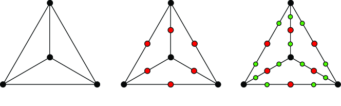
Figure 1: $K_{4}$, $s(K_{4})$ and $s^{2}(K_{4})$. Black vertices denote the initial vertices of $K_{4}$ while red and green vertices are those introduced to obtain $s(K_{4})$ and $s^{2}(K_{4})$, respectively.

Definition 2.2.

The circuit rank or cyclomatic number of $G$ is the minimum number $r$ of edges that have to be removed from $G$ to convert the graph into a tree.

Obviously, the circuit rank of $G$ is $r=E_{0}-N_{0}+1$.

Lemma 2.3.

The circuit rank of $s^{n}(G)$ and $G$ are the same for $n\geqslant 0$.

Proof.   From the definition of the subdivision graph and (1), the circuit rank of $s^{n}(G)$ is $r=E_{n}-N_{n}+1=E_{0}-N_{0}+1$.  $\Box$

Given the subdivision graph $s^{n}(G)$ we label its nodes from $1$ to $N_{n}$. Let $d_{i}$ be the degree of vertex $i$, then $D_{n}=\mbox{diag}(d_{1},d_{2},\cdots,d_{N_{n}})$ denotes the diagonal degree matrix of $s^{n}(G)$ and $A_{n}$ its adjacency matrix, defined as a matrix with the $(i,j)$-entry equal to $1$ if vertices $i$ and $j$ are adjacent and $0$ otherwise.

We introduce now the probability transition matrix for random walks on $s^{n}(G)$ or Markov matrix as $M_{n}=D_{n}^{-1}A_{n}$. $M_{n}$ can be normalized to obtain a symmetric matrix $P_{n}$.

$$P_{n}=D_{n}^{-\frac{1}{2}}A_{n}D_{n}^{-\frac{1}{2}}=D_{n}^{\frac{1}{2}}M_{n}D_{n}^{-\frac{1}{2}}\,.$$ (2)

The $(i,j)$th entry of $P_{n}$ is $(P_{n})_{ij}=\frac{A_{n}(i,j)}{\sqrt{d_{i}d_{j}}}$.

Definition 2.4.

The normalized Laplacian matrix of $s^{n}(G)$ is

$${\cal L}_{n}=I-D_{n}^{\frac{1}{2}}M_{n}D_{n}^{-\frac{1}{2}}=I-P_{n},$$ (3)

where $I$ is the identity matrix with the same order as $P_{n}$.

We denote the spectrum of ${\cal L}_{n}$ by $\sigma_{n}=\left\{\lambda^{(n)}_{1},\lambda^{(n)}_{2},\cdots,\lambda^{(n)}_{N_{n}}\right\}$. It is known that $0=\lambda_{1}^{(n)}<\lambda_{2}^{(n)}\leqslant\cdots\leqslant\lambda_{N_{n}-1}^{(n)}\leqslant\lambda_{N_{n}}^{(n)}\leqslant 2$. The spectrum of the normalized Laplacian matrix of a graph provides us with relevant structural information about the graph, see [7, 16].

Below, we will then relate $\sigma_{n}$ to some significant invariants of $s^{n}(G)$.

Definition 2.5.

Replacing each edge of a simple connected graph $G$ by a unit resistor, we obtain an electrical network $G^{*}$ corresponding to $G$. The resistance distance $r_{ij}$ between vertices $i$ and $j$ of $G$ is equal to the effective resistance between the two equivalent vertices of $G^{*}$ [17].

Definition 2.6.

The multiplicative degree-Kirchhoff index of $G$ is defined as [18]:

$${K\!f}^{*}(G)=\sum_{i<j}d_{i}d_{j}r_{ij}.$$ (4)

This index is different from the classical Kirchhoff index [19], ${K\!f}(G)=\sum_{i<j}r_{ij}$, as it takes into account the degree distribution of the graph.

It has been proved [18] that ${K\!f}^{*}(G)$ can be obtained from the spectrum $\sigma_{0}=\{\lambda_{1},\lambda_{2},\cdots,\lambda_{N_{0}}\}$ of the normalized Laplacian matrix ${\cal L}_{0}$ of $G$:

$${K\!f}^{*}(G)=2E_{0}\sum_{k=2}^{N_{0}}\frac{1}{\lambda_{k}},$$ (5)

where $0=\lambda_{1}<\lambda_{2}\leqslant\cdots\leqslant\lambda_{N_{0}}\leqslant 2$.

Thus, for $n\geqslant 0$, we have:

$${K\!f}^{*}(s^{n}(G))=2E_{n}\sum_{k=2}^{N_{n}}\frac{1}{\lambda^{(n)}_{k}},$$ (6)

where $0=\lambda_{1}^{(n)}<\lambda_{2}^{(n)}\leqslant\cdots\leqslant\lambda_{N_{n}-1}^{(n)}\leqslant\lambda_{N_{n}}^{(n)}\leqslant 2$ are the eigenvalues of ${\cal L}_{n}$.

Definition 2.7.

Given a graph $G$, the Kemeny’s constant $K(G)$, also known as average hitting time, is the expected number of steps required for the transition from a starting vertex $i$ to a destination vertex, which is chosen randomly according to a stationary distribution of unbiased random walks on $G$, see [20] for more details.

It is known that $K(G)$ is a constant as it is independent of the selection of starting vertex $i$, see [12]. Moreover, the Kemeny’s constant can be computed from the normalized Laplacian spectrum in a very simple way as the sum of all reciprocal eigenvalues, except $1/\lambda_{1}$, see [16]. Thus, we can write, for $s^{n}(G)$ and $\sigma_{n}$:

$$K(s^{n}(G))=\sum_{k=2}^{N_{n}}\frac{1}{\lambda^{(n)}_{k}}.$$ (7)

The last graph invariant considered in this paper is the number of spanning trees of a graph $G$. A spanning tree is a subgraph of $G$ that includes all the vertices of $G$ and is a tree. A known result from Chung [7] allows the calculation of this number from the normalized Laplacian spectrum and the degrees of all the vertices, thus the number of spanning trees $N_{\rm st}^{(n)}$ of $s^{n}(G)$ is

$$N_{\rm st}^{(n)}=\frac{\displaystyle\prod_{i=1}^{N_{n}}d_{i}\prod_{i=2}^{N_{n}}\lambda_{i}^{(n)}}{\displaystyle\sum_{i=1}^{N_{n}}d_{i}}\,.$$ (8)

In the next section we provide an analytical expression for this invariant for any value of $n\geqslant 0$.

3 Normalized Laplacian spectrum of the subdivision graph $s^{n}(G)$

In this section we find an analytical expression for the spectrum $\sigma_{n}$ of ${\cal L}_{n}(s^{n}(G))$, the normalized Laplacian of the subdivision graph $s^{n}(G)$. We show that this spectrum can be obtained iteratively from the spectrum of $G$. As ${\cal L}_{n}=I-P_{n}$, if $\mu$ is an eigenvalue of $P_{n}$ then $1-\mu$ is an eigenvalue of ${\cal L}_{n}$ with the same multiplicity. We denote the multiplicity of $\mu$ as $m_{P_{n}}(\mu)$. Thus we calculate first the spectrum $\sigma^{\prime}_{n}$ of $P_{n}$.

Lemma 3.1.

Let $\mu$ be any nonzero eigenvalue of $P_{n}$ and let ${R}(x)=2x^{2}-1$. Then, ${R}(\mu)$ is an eigenvalue of $P_{n-1}$ with the same multiplicity as $\mu$.

Proof.   Divide the vertices of $s^{n}(G)$ into two groups ${V}_{\rm old}^{n}$ and ${V}_{\rm new}^{n}$, where ${V}_{\rm new}^{n}$ contains all the vertices created when the edges of $s^{n-1}(G)$ are subdivided to generate $s^{n}(G)$ and ${V}_{\rm old}^{n}$ contains the rest. Obviously, ${V}_{\rm old}^{n}$ has the same vertices as $s^{n-1}(G)$. Thus for convenience, in the following when any vertex of ${V}_{\rm old}^{n}$ is considered, it also refers to the corresponding vertex of $s^{n-1}(G)$.

Let $\psi=(\psi_{1},\psi_{2},\ldots,\psi_{N_{n}})^{\top}$ be any eigenvector associated to an eigenvalue $\mu$ of $P_{n}$. Hence

$$P_{n}\psi=\mu\psi$$ (9)

Consider a vertex $i\in{V}_{\rm old}^{n}$ of $s^{n}(G)$ and denote $\mathcal{N}$ the set of all its neighbors in $s^{n}(G)$ and $\mathcal{N}^{\prime}$ the set of all its neighbors in $s^{n-1}(G)$. From the definition of subdivision graph, there exists a bijection between $\mathcal{N}$ and $\mathcal{N}^{\prime}$. If we rewrite Eq. (9) as $\sum_{j=1}^{N_{n}}(P_{n})_{ij}\psi_{j}=\mu\psi_{i},$ we have

$$\mu\psi_{i}=\sum_{j\in\mathcal{N}}\frac{1}{\sqrt{d_{i}d_{j}}}\psi_{j}=\sum_{j\in\mathcal{N}}\frac{1}{\sqrt{2d_{i}}}\psi_{j}.$$ (10)

For any vertex $j\in\mathcal{N}$, we have a similar relation

$$\mu\psi_{j}=\sum_{k=1}^{N_{n}}(P_{n})_{jk}\psi_{k}=\frac{1}{\sqrt{2d_{i}}}\psi_{i}+\frac{1}{\sqrt{2d_{j^{\prime}}}}\psi_{j^{\prime}}.$$ (11)

where vertex $j^{\prime}\in\mathcal{N}^{\prime}$ is the other neighbor of vertex $j$ in $s^{n}(G)$ . Combining Eq. (10) and Eq. (11) yields

$$\begin{split}\mu\psi_{i}&=\frac{1}{\mu\sqrt{2d_{i}}}\times\sum_{j^{\prime}\in\mathcal{N}^{\prime}}\left(\frac{1}{\sqrt{2d_{i}}}\psi_{i}+\frac{1}{\sqrt{2d_{j^{\prime}}}}\psi_{j^{\prime}}\right)\\ &=\frac{1}{\mu\sqrt{2d_{i}}}\times\left(\frac{d_{i}}{\sqrt{2d_{i}}}\psi_{i}+\sum_{j^{\prime}\in\mathcal{N}^{\prime}}\frac{1}{\sqrt{2d_{j^{\prime}}}}\psi_{j^{\prime}}\right).\end{split}$$ (12)

Therefore,

$$(2\mu^{2}-1)\psi_{i}=\sum_{j^{\prime}\in\mathcal{N}^{\prime}}\frac{1}{\sqrt{d_{i}d_{j^{\prime}}}}\psi_{j^{\prime}}.$$ (13)

Eq. (13) directly reflects that ${R}(\mu)=(2\mu^{2}-1)$ is an eigenvalue of $P_{n-1}$, $\psi_{o}=(\psi_{i})_{i\in{V}_{\rm old}^{n}}^{\top}$ is one of its corresponding eigenvectors and $\psi$ can be totally determined by $\psi_{o}$ by using Eq. (11). Hence $m_{P_{n-1}}(R(\mu))\geqslant m_{P_{n}}(\mu)$.

Suppose now that $m_{P_{n-1}}(R(\mu))>m_{P_{n}}(\mu)$. Then there exists an extra eigenvector $\psi_{e}$ associated to ${R}(\mu)$ without an associated eigenvector in $P_{n}$. But Eq. (11) provides $\psi_{e}$ with its corresponding eigenvector in $P_{n}$ as $\mu$ is nonzero, in contradiction with our assumption. Thus $m_{P_{n-1}}(R(\mu))=m_{P_{n}}(\mu)$ and the proof is completed.  $\Box$

Lemma 3.2.

Let $\mu$ be any eigenvalue of $P_{n-1}$ such that $\mu\neq-1$ and let $f_{1}(x)=\sqrt{\frac{x+1}{2}}$ and $f_{2}(x)=-\sqrt{\frac{x+1}{2}}$. Then $f_{1}(\mu)$ and $f_{2}(\mu)$ are eigenvalues of $P_{n}$. Besides, $m_{P_{n}}(f_{1}(\mu))=m_{P_{n}}(f_{2}(\mu))=m_{P_{n-1}}(\mu)$.

Proof.   This lemma is a direct consequence of Lemma 3.1  $\Box$

Remark 3.3.

Lemmas 3.1 and 3.2 indicate that any nonzero eigenvalues of $P_{n}$ can be obtained from the spectrum of $P_{n-1}$. Due to the simple expression of $R$, $f_{1}$ and $f_{2}$, we easily find that each eigenvalue, except $-1$, of $P_{n-1}$ will generate two unique eigenvalues of $P_{n}$. Thus $2(N_{n-1}-m_{P_{n-1}}(-1))$ eigenvalues of $\sigma^{\prime}_{n}$, and consequently of $\sigma_{n}$, are determined this way.

The Perron-Frobenius theorem [21] shows that the largest absolute value of the eigenvalues of $P_{n}$ is always 1. And because of the existence of a unique stationary distribution for random walks on $s^{n}(G)$, the multiplicity of the eigenvalue $1$ is always $1$ for any $n\geqslant 0$. Since $f_{2}(1)=-1$, we also obtain $m_{P_{n}}(-1)=1$ for any $n\geqslant 1$. This can be further explained from the perspective of Markov chains. Since $s^{n}(G)$ is a bipartite graph [22] containing no odd-length cycles for any $n>0$, random walks on it are periodic with period $2$, which means it takes an even number of steps to return to the starting vertex. Thus the smallest eigenvalue of the Markov matrix of $s^{n}(G)$ is $-1$ [23]. But random walks on a general graph $G$ can be aperiodic [24] if the graph has an odd-length cycle. Hence the multiplicity of the eigenvalue $-1$ of $P_{0}$ depends on the structure of $G$ [23].

Lemmas 3.1 and 3.2 allow us to obtain the transition between the eigenvalues of the normalized Laplacian of $s^{n}(G)$ at each iteration step. If $\mu$ is an eigenvalue of $P_{n}$ then $\lambda=1-\mu$ is an eigenvalue of ${\cal L}_{n}$. Let $Q(x)=4x-2x^{2}$, by Lemma 3.1, $Q(\lambda)=1-R(1-\lambda)$ is an eigenvalue of ${\cal L}_{n-1}$ if $\lambda\neq 1$. This allows us to state the following lemma:

Lemma 3.4.

Let $\lambda$ be any eigenvalue of ${\cal L}_{n-1}$ such that $\lambda\neq 2$ and let $g_{1}(x)=1+\sqrt{1-\frac{x}{2}}$ and $g_{2}(x)=1-\sqrt{1-\frac{x}{2}}$ . Then $g_{1}(\lambda)$ and $g_{2}(\lambda)$ are eigenvalues of ${\cal L}_{n}$ and $m_{{\cal L}_{n}}(g_{1}(\lambda))=m_{{\cal L}_{n}}(g_{2}(\lambda))=m_{{\cal L}_{n-1}}(\lambda)$.

$\Box$

Definition 3.5.

Let $U=\{u_{1},u_{2},\cdots,u_{k}\}$ be any finite multiset of real number where $|u_{i}|\leqslant 1$ for $i\in[1,k]$. The multisets $\mathcal{R}^{-1}(U)$ and $\mathcal{Q}^{-1}(U)$ are defined as

$$\mathcal{R}^{-1}(U)=\{f_{1}(u_{1}),f_{2}(u_{1}),f_{1}(u_{2}),f_{2}(u_{2}),\cdots,f_{1}(u_{k}),f_{2}(u_{k})\};$$ (14)

$$\mathcal{Q}^{-1}(U)=\{g_{1}(u_{1}),g_{2}(u_{1}),g_{1}(u_{2}),g_{2}(u_{2}),\cdots,g_{1}(u_{k}),g_{2}(u_{k})\}.$$ (15)

Our main result in this section is the following theorem.

Lemma 3.6.

The spectrum $\sigma^{\prime}_{n}$ of $P_{n}$, for $n>0$, is:

$$\sigma^{\prime}_{n}=\mathcal{R}^{-1}\left(\sigma^{\prime}_{n-1}\setminus\{-1\}\right)\cup\{\underbrace{0,\cdots,0}_{\text{$m_{P_{n}}(0)$}}\}$$ (16)

When $n>1$, $m_{P_{n}}(0)=r+1$. When $n=1$, if G contains any odd-length cycle then $m_{P_{n}}(0)=r-1$, otherwise $m_{P_{n}}(0)=r+1$, where $r$ is the circuit rank of $G$.

Proof.   Combining Lemma 3.1, Lemma 3.2 and considering Remark 3.3, the multiplicity of the eigenvalue $0$ of $P_{n}$ can be determined indirectly:

$$\begin{split}m_{P_{n}}(0)&=N_{n}-2(N_{n-1}-m_{P_{n-1}}(-1))\\ &=E_{0}-N_{0}+2\cdot m_{P_{n-1}}(-1).\end{split}$$ (17)

Based on the previous results, it is obvious that $m_{P_{n-1}}(-1)=0$ if and only if $n=1$ and G contains an odd-length cycle, otherwise $m_{P_{n-1}}(-1)=1$, which completes the proof.  $\Box$

This result allows us to state the main result of this section.

Theorem 3.7.

The spectra $\sigma_{n}$ of ${\cal L}_{n}$ is obtained from $\sigma_{n-1}$ of ${\cal L}_{n-1}$ as:

$$\sigma_{n}=\mathcal{Q}^{-1}\left(\sigma_{n-1}\setminus\{2\}\right)\cup\{\underbrace{1,\cdots,1}_{\text{$m_{{\cal L}_{n}}(1)$}}\}$$ (18)

for $n>0$ and where $m_{{\cal L}_{n}}(1)=m_{P_{n}}(0)$ is the multiplicity of the eigenvalue $1$ of ${\cal L}_{n}$.

$\Box$

Due to the particularity of the eigenvalue $1$ of ${\cal L}_{n}$, we call it the exceptional eigenvalue [25] of the family of matrices $\{{\cal L}_{n}\}$ whose spectra show self-similar characteristics. For many other family of graphs [25, 26] with a similar self-similar property with respect to the spectra of their Markov matrices, the multiplicity of exceptional eigenvalues grows fast as $n$ increases. However, for the normalized Laplacian of subdivision graphs $\{s^{n}(G)\}$, the multiplicity of the only exceptional eigenvalue $1$ is always $r+1$ for $n>1$.

4 Application of the spectrum of subdivision graph

In this section we use the spectra of ${\cal L}_{n}$, the normalized Laplacian of the subdivision graph $s^{n}(G)$, to compute some relevant invariants related to the structure of $s^{n}(G)$. Thus, we give closed formulas for the multiplicative degree-Kirchhoff index, Kemeny’s constant and the number of spanning trees of $s^{n}(G)$. These results depend only on $n$ and some invariants of the original graph $G$.

4.1 Multiplicative degree-Kirchhoff index

Theorem 4.1.

The multiplicative degree-Kirchhoff indices of $s^{n}(G)$ and $s^{n-1}(G)$ are related as follows, for any $n>0$:

$${K\!f}^{*}(s^{n}(G))=8{K\!f}^{*}(s^{n-1}(G))+2^{n}(2r-1)E_{0}.$$ (19)

Therefore, the general expression for ${K\!f}^{*}(s^{n}(G))$ is

$${K\!f}^{*}(s^{n}(G))=8^{n}{K\!f}^{*}(G)+\frac{8^{n}-2^{n}}{3}(2r-1)E_{0}.$$ (20)

Proof.   From Eq. (6) and Corollary 3.7, the relation between ${K\!f}^{*}(s^{n}(G))$ and ${K\!f}^{*}(s^{n-1}(G))$ can be expressed as:

$$\begin{split}{K\!f}^{*}(s^{n}(G))&=2E_{n}\left(\frac{1}{\lambda^{(n)}_{N_{n}}}+\frac{m_{{\cal L}_{n}}(0)}{1-0}+\sum_{k=2}^{N_{n-1}-1}\left(\frac{1}{g_{1}(\lambda_{k}^{(n-1)})}+\frac{1}{g_{2}(\lambda_{k}^{(n-1)})}\right)\right)\\ &=2E_{n}\left(\frac{1}{2}+(r+1)+4\sum_{k=2}^{N_{n-1}-1}\frac{1}{\lambda_{k}^{(n-1)}}\right)\\ &=2E_{n}\left(\frac{1}{2}+(r+1)+4\left(\frac{K(s^{n-1}(G))}{2E_{n-1}}-\frac{1}{2}\right)\right)\\ &=8{K\!f}^{*}(s^{n-1}(G))+2^{n}(2r-1)E_{0},\end{split}$$ (21)

provided that $m_{{\cal L}_{n-1}}(-1)=1$, where $\lambda_{k}^{(n)}$ represents the eigenvalue of ${\cal L}_{n}$.

When $n=1$ and $m_{{\cal L}_{n}}{0}(-1)=0$, we obtain:

$$\begin{split}{K\!f}^{*}(s(G))&=2E_{1}\left(\frac{1}{\lambda_{N_{1}}}+\frac{m_{{\cal L}_{1}}(0)}{1-0}+\sum_{k=2}^{N_{0}}\left(\frac{1}{g_{1}(\lambda_{k})}+\frac{1}{g_{2}(\lambda_{k})}\right)\right)\\ &=2E_{1}\left(\frac{1}{2}+(r-1)+4\sum_{k=2}^{N_{0}}\frac{1}{\lambda_{k}}\right)\\ &=2E_{1}\left(\frac{1}{2}+(r-1)+4\cdot\frac{K(G)}{2E_{0}}\right)\\ &=8{K\!f}^{*}(G)+2(2r-1)E_{0}.\end{split}$$ (22)

The similarity of Eq. (21) and Eq. (22) indicates that Eq. (19) holds for any simple connected graph $G$ for $n>0$.

Transforming Eq. (19) into

$${K\!f}^{*}(s^{n}(G))+\frac{2^{n}(2r-1)E_{0}}{3}=8\left(K(s^{n-1}(G))+\frac{2^{n-1}(2r-1)E_{0}}{3}\right)$$ (23)

yields

$${K\!f}^{*}(s^{n}(G))=8^{n}{K\!f}^{*}(G)+\frac{8^{n}-2^{n}}{3}(2r-1)E_{0}.$$ (24)

$\Box$

We note here that this expression has been also obtained recently by Yang and Klein [27] by using a counting methodology not related with spectral techniques. Our result confirms both their calculation and the usefulness of the concise spectral methods described here.

4.2 Kemeny’s constant

Theorem 4.2.

The Kemeny’s constant for random walks on $s^{n}(G)$ can be obtained from $K(s^{n-1}(G))$ through

$$K(s^{n}(G))=4K\left(s^{n-1}(G)\right)+r-\frac{1}{2}.$$ (25)

The general expression is

$$K(s^{n}(G))=4^{n}K(G)+\frac{4^{n}-1}{3}\left(r-\frac{1}{2}\right).$$ (26)

Proof.   Theorem 4.2 is an obvious consequence of Theorem 4.1 considering Eq. (7).  $\Box$

4.3 Spanning trees

Theorem 4.3.

The number of spanning trees of $s^{n}(G)$ is, for any $n>0$:

$$N_{\rm st}^{(n)}=2^{r}N_{\rm st}^{(n-1)}=2^{rn}N_{\rm st}^{(0)}.$$ (27)

Proof.   From Eq. (8) and the properties of the subdivision of a graph:

$$\frac{N_{\rm st}^{(n)}}{N_{\rm st}^{(n-1)}}=2^{E_{n-1}-1}\times\tfrac{\prod\limits_{i=2}^{N_{n}}\lambda_{i}^{(n)}}{\prod\limits_{i=2}^{N_{n-1}}\lambda_{i}^{(n-1)}}.$$ (28)

Here $\lambda_{i}^{(n)}$ are the eigenvalues of ${\cal L}_{n}$

Then, by the same techniques used in the previous subsection, we obtain

$$\begin{split}\prod\limits_{i=2}^{N_{n}}\lambda_{i}^{(n)}&=2\times\prod\limits_{i=2}^{N_{n-1}-1}\Big{(}g_{1}\big{(}\lambda_{i}^{(n-1)}\big{)}g_{2}\big{(}\lambda_{i}^{(n-1)}\big{)}\Big{)}\\ &=2\times\prod\limits_{i=2}^{N_{n-1}-1}\frac{\lambda_{i}^{(n-1)}}{2}\\ &=\frac{1}{2^{N_{n-1}-2}}\prod\limits_{i=2}^{N_{n-1}}\lambda_{i}^{(n-1)}\end{split}$$ (29)

if $m_{{\cal L}_{n-1}}(-1)=1$.

When $n=1$ and $m_{{\cal L}_{0}}(-1)=1$, the relation becomes

$$\begin{split}\prod\limits_{i=2}^{N_{1}}\lambda_{i}&=2\times\prod\limits_{i=2}^{N_{0}}\Big{(}g_{1}\big{(}\lambda_{i}\big{)}g_{2}\big{(}\lambda_{i}\big{)}\Big{)}\\ &=2\times\prod\limits_{i=2}^{N_{0}}\frac{\lambda_{i}}{2}\\ &=\frac{1}{2^{N_{0}-2}}\prod\limits_{i=2}^{N_{0}}\lambda_{i}\end{split}$$ (30)

which coincides with Eq. (29).

Therefore, the equality

$$N_{\rm st}^{(n)}=2^{E_{n-1}-N_{n-1}+1}\times N_{\rm st}^{(n-1)}=2^{r}N_{\rm st}^{(n-1)}=2^{rn}N_{\rm st}^{(0)}$$ (31)

holds for any $n>0$ as the circuit rank $r$ remains unchanged.  $\Box$

5 Conclusion

In this study we have focused on the analytical calculation of $\sigma_{n}$, the spectra for the normalized Laplacian of iterated subdivisions of any simple connected graph. This was possible through the analysis of the eigenvectors corresponding to adjacent vertices at different iteration steps. Our methods could be also applied to find the spectra of other graph families constructed iteratively.

The simple relationship between the spectrum of the Markov and the normalized Laplacian matrices of a subdivision graph facilitates the calculations to obtain the exact distribution and values of all eigenvalues. One particular interesting result is that the multiplicity of the exceptional eigenvalues of $\sigma_{n}$ do not increase exponentially with $n$ as in [28, 29] but is a constant determined by the value of the circuit rank of the initial graph.

The calculation of the multiplicative degree-Kirchhoff index, Kemeny’s constant and the number of spanning trees in section 4 is also succinct, if we compare it to other methods, thanks to the knowledge of the full spectrum of $P_{n}$ or ${\cal L}_{n}$. The expressions found can be directly used in the analysis of subdivisions of any simple connected graph while only needing minimal structural information from it, and this is part of the value of our study.

References

- Dasgupta et al. [2004] A. Dasgupta, J. E. Hopcroft, F. McSherry, Spectral analysis of random graphs with skewed degree distributions, in: Proc. 45th Annual IEEE Symposium on Foundations of Computer Science, 2004, pp. 602–610.
- Spielman [2007] D. A. Spielman, Spectral graph theory and its applications, in: Proc. 48th Annual IEEE Symposium on Foundations of Computer Science, 2007, pp. 29–38.
- Tran et al. [2013] L. V. Tran, V. H. Vu, K. Wang, Sparse random graphs: Eigenvalues and eigenvectors, Rand. Struct. Alg. 42 (2013) 110–134.
- Cvetković and Simić [2011] D. Cvetković, S. Simić, Graph spectra in computer science, Linear Algebra Appl. 434 (2011) 1545–1562.
- Arsić et al. [2012] B. Arsić, D. Cvetković, S. K. Simić, M. Škarić, Graph spectral techniques in computer sciences, Appl. Anal. Discrete Math. 6 (2012) 1–30.
- Godsil and Royle [2001] C. D. Godsil, G. Royle, Algebraic Graph Theory, Graduate Texts in Mathematics, Springer New York, 2001.
- Chung [1997] F. R. Chung, Spectral Graph Theory, American Mathematical Society, Providence, RI, 1997.
- Brouwer and Haemers [2012] A. E. Brouwer, W. H. Haemers, Spectra of Graphs, Universitext, Springer New York, 2012.
- Lovász [1993] L. Lovász, in: D. Miklós, V. T. Sós, T. Szönyi (Eds.), Random walks on graphs: a survey, volume 2 of Combinatorics, Paul Erdös is Eighty, János Bolyai Mathematical Society, Budapest, 1993, pp. 1–46.
- Zhang et al. [2013] Z. Zhang, T. Shan, G. Chen, Random walks on weighted networks, Phys. Rev. E 87 (2013) 012112.
- Kemeny and Snell [1976] J. G. Kemeny, J. L. Snell, Finite Markov Chains, Springer, New York, 1976.
- Levene and Loizou [2002] M. Levene, G. Loizou, Kemeny’s constant and the random surfer, Amer. Math. Monthly 109 (2002) 741–745.
- Chen et al. [2004] G. Chen, G. Davis, F. Hall, Z. Li, K. Patel, M. Stewart, An interlacing result on normalized Laplacians, SIAM J. Discrete Math. 18 (2004) 353–361.
- Blumen et al. [2003] A. Blumen, A. Jurjiu, T. Koslowski, C. von Ferber, Dynamics of Vicsek fractals, models for hyperbranched polymers, Phys. Rev. E 67 (2003) 061103.
- Shirai [1999] T. Shirai, The spectrum of infinite regular line graphs, Trans. Amer. Math. Soc. 352 (1999) 115–132.
- Butler [2016] S. Butler, Algebraic aspects of the normalized Laplacian, in: A. Beveridge, J. Griggs, L. Hogben, G. Musiker, P. Tetali (Eds.), Recent Trends in Combinatorics, volume to appear of The IMA Volumes in Mathematics and its Applications, IMA, 2016.
- Klein and Randić [1993] D. J. Klein, M. Randić, Resistance distance, J. Math. Chem. 12 (1993) 81–95.
- Chen and Zhang [2007] H. Chen, F. Zhang, Resistance distance and the normalized Laplacian spectrum, Discrete Appl. Math. 155 (2007) 654–661.
- Bonchev et al. [1994] D. Bonchev, A. T. Balaban, X. Liu, D. J. Klein, Molecular cyclicity and centricity of polycyclic graphs. I. Cyclicity based on resistance distances or reciprocal distances, Int. J. Quant. Chem. 50 (1994) 1–20.
- Hunter [2014] J. J. Hunter, The role of Kemeny’s constant in properties of Markov chains, Commun. Statist. Theor. Meth. 43 (2014) 1309–1321.
- Friedland et al. [2013] S. Friedland, S. Gaubert, L. Han, Perron–Frobenius theorem for nonnegative multilinear forms and extensions, Linear Algebra Appl. 438 (2013) 738–749.
- Asratian et al. [1998] A. S. Asratian, T. M. Denley, R. Häggkvist, Bipartite graphs and their applications, 131, Cambridge University Press, 1998.
- Zhang [2004] X.-D. Zhang, The smallest eigenvalue for reversible Markov chains, Linear Algebra Appl. 383 (2004) 175–186.
- Diaconis and Stroock [1991] P. Diaconis, D. Stroock, Geometric bounds for eigenvalues of Markov chains, Ann. Appl. Probab. (1991) 36–61.
- Bajorin et al. [2008] N. Bajorin, T. Chen, A. Dagan, C. Emmons, M. Hussein, M. Khalil, P. Mody, B. Steinhurst, A. Teplyaev, Vibration modes of 3n-gaskets and other fractals, J. Phys. A: Math. Theor. 41 (2008) 015101.
- Teplyaev [1998] A. Teplyaev, Spectral analysis on infinite Sierpiński gaskets, J. Funct. Anal. 159 (1998) 537–567.
- Yang and Klein [2015] Y. Yang, D. J. Klein, Resistance distance-based graph invariants of subdivisions and triangulations of graphs, Discrete Appl. Math. 181 (2015) 260–274.
- Xie et al. [2015] P. Xie, Y. Lin, Z. Zhang, Spectrum of walk matrix for Koch network and its application, J. Chem. Phys. 142 (2015) 224106.
- Zhang et al. [2014] Z. Zhang, X. Guo, Y. Lin, Full eigenvalues of the Markov matrix for scale-free polymer networks, Phys. Rev. E 90 (2014) 022816.