Inverse boundary value problem for the Helmholtz equation: quantitative conditional Lipschitz stability estimates

Abstract

We study the inverse boundary value problem for the Helmholtz equation using the Dirichlet-to-Neumann map at selected frequencies as the data. A conditional Lipschitz stability estimate for the inverse problem holds in the case of wavespeeds that are a linear combination of piecewise constant functions (following a domain partition) and gives a framework in which the scheme converges. The stability constant grows exponentially as the number of subdomains in the domain partition increases. We establish an order optimal upper bound for the stability constant. We eventually realize computational experiments to demonstrate the stability constant evolution for three dimensional wavespeed reconstruction.

simaxxxxxxxx–x

35R30, 86A22, 65N12, 35J25

1 Introduction

In this paper we study the inverse boundary value problem for the Helmholtz equation using the Dirichlet-to-Neumann map at selected frequencies as the data. This inverse problem arises, for example, in reflection seismology and inverse obstacle scattering problems for electromagnetic waves [3, 22, 4]. We consider wavespeeds containing discontinuities.

Uniqueness of the mentioned inverse boundary value problem was established by Sylvester & Uhlmann [21] assuming that the wavespeed is a bounded measurable function. This inverse problem has been extensively studied from an optimization point of view. We mention, in particular, the work of [5].

It is well known that the logarithmic character of stability of the inverse boundary value problem for the Helmholtz equation [1, 19] cannot be avoided, see also [14, 15]. In fact, in [17] Mandache proved that despite of regularity a priori assumptions of any order on the unknown wavespeed, logarithmic stability is the best possible. However, conditional Lipschitz stability estimates can be obtained: accounting for discontinuities, such an estimate holds if the unknown wavespeed is a finite linear combination of piecewise constant functions with an underlying known domain partitioning [6]. It was obtained following an approach introduced by Alessandrini and Vessella [2] and further developed by Beretta and Francini [7] for Electrical Impedance Tomography (EIT) based on the use of singular solutions. If, on one hand, this method allows to use partial data, on the other hand it does not allow to find an optimal bound of the stability constant. Here, we revisit the Lipschitz stability estimate for the full Dirichlet-to-Neumann map using complex geometrical optics (CGO) solutions which give rise to a sharp upper bound of the Lipschitz constant in terms of the number of subdomains in the domain partitioning. We develop the estimate in $L^{2}(\Omega)$.

Unfortunately, the use of CGO’s solutions leads naturally to a dependence of the stability constant on frequency of exponential type. This is clearly far from being optimal as it is also pointed out in the paper of Nagayasu, Uhlmann and Wang [18]. There the authors prove a stability estimate, in terms of Cauchy data instead of the Dirichlet-to-Neumann map using CGO solutions. They derive a stability estimate consisting of two parts: a Lipschitz stability estimate and a Logarithmic stability estimate. When the frequency increases the logarithmic part decreases while the Lipschitz part becomes dominant but with a stability constant which blows up exponentially in frequency.

We can exploit the quantitative stability estimate, via a Fourier transform, in the corresponding time-domain inverse boundary value problem with bounded frequency data. Datchev and De Hoop [9] showed how to choose classes of non-smooth coefficient functions, one of which is consistent with the class considered here, so that optimization formulations of inverse wave problems satisfy the prerequisites for application of steepest descent and Newton-type iterative reconstruction methods. The proof is based on resolvent estimates for the Helmholtz equation. Thus, one can allow approximate localization of the data in selected time windows, with size inversely proportional to the maximum allowed frequency. This is of importance to applications in the context of reducing the complexity of field data. We note that no information is lost by cutting out a (short) time window, since the boundary source functions (and wave solutions), being compactly supported in frequency, are analytic with respect to time. We cannot allow arbitrarily high frequencies in the data. This restriction is reflected, also, in the observation by Blazek, Stolk & Symes [8] that the adjoint equation, which appears in the mentioned iterative methods, does not admit solutions.

As a part of the analysis, we study the Fréchet differentiability of the direct problem and obtain the frequency and domain partitioning dependencies of the relevant constants away from the Dirichlet spectrum. Our results hold for finite fixed frequency data including frequencies arbitrarily close to zero while avoiding Dirichlet eigenfrequencies; in view of the estimates, inherently, there is a finest scale which can be reached. Finally we estimate the stability numerically and demonstrate the validity of the bounds, in particular in the context of reflection seismology.

2 Inverse boundary value problem with the Dirichlet-to-Neumann map as the data

2.1 Direct problem and forward operator

We describe the direct problem and some properties of the data, that is, the Dirichlet-to-Neumann map. We will formulate the direct problem as a nonlinear operator mapping $F_{\omega}$ from $L^{\infty}(\Omega)$ to $\mathcal{L}(H^{1/2}(\partial\Omega),H^{-1/2}(\partial\Omega))$ defined as

$$F_{\omega}(c^{-2})=\Lambda_{\omega^{2}c^{-2}},$$

where $\Lambda_{\omega^{2}c^{-2}}$ indicates the Dirichlet to Neumann operator. Indeed, at fixed frequency $\omega^{2}$, we consider the boundary value problem,

(1) $$\left\{\begin{array}[]{rl}(-\Delta-\omega^{2}c^{-2}(x))u=&0,\quad\mbox{ in }\Omega,\\ u=&g\quad\mbox{ on }\partial\Omega,\end{array}\right.$$

while $\Lambda_{\omega^{2}c^{-2}}:\ g\to\frac{\partial u}{\partial\nu}|_{\partial\Omega}$, where $\nu$ denotes the outward unit normal vector to $\partial\Omega$. In this section, we will state some known results concerning the well-posedness of problem Eq. 1 (see, for example, [12]) and regularity properties of the nonlinear map $F_{\omega}$. We will sketch the proofs of these results because we will need to keep track of the dependencies of the constants involved on frequency. We invoke

Assumption .

There exist two positive constants $B_{1},B_{2}$ such that

(2) $$B_{1}\leq c^{-2}\leq B_{2}\quad\text{in }\Omega.$$

In the sequel of Section 2 $C=C(a,b,c,\dots)$ indicates that $C$ depends only on the parameters $a,b,c,\dots$ and we will indicate different constants with the same letter $C$.

Proposition 2.1.

Let $\Omega$ be a bounded Lipschitz domain in $\mathbb{R}^{3}$, $f\in L^{2}(\Omega)$, $g\in H^{1/2}(\partial\Omega)$ and $c^{-2}\in L^{\infty}(\Omega)$ satisfying Section 2.1. Then, there exists a discrete set $\Sigma_{c^{-2}}:=\{\tilde{\lambda}_{n}\quad|\tilde{\lambda}_{n}>0,\ \forall n\in\mathbb{N}\}$ such that, for every $\omega^{2}\in\mathbb{C}\backslash\Sigma_{c^{-2}}$, there exists a unique solution $u\in H^{1}(\Omega)$ of

(3) $$\left\{\begin{array}[]{rl}(-\Delta-\omega^{2}c^{-2}(x))u=&f\ \ \quad\mbox{ in }\Omega,\\ u=&g\quad\mbox{ on }\partial\Omega.\end{array}\right.$$

Furthermore, there exists a positive constant $C$ such that

(4) $$\|u\|_{H^{1}(\Omega)}\leq C\left(1+\frac{\omega^{2}}{\textrm{d}(\omega^{2},\Sigma_{c^{-2}})}\right)\left(\|g\|_{H^{1/2}(\partial\Omega)}+\|f\|_{L^{2}(\Omega)}\right),$$

where $C=C(\Omega,B_{2})$ and $\textrm{d}(\omega^{2},\Sigma_{c^{-2}})$ indicates the distance of $\omega^{2}$ from $\Sigma_{c^{-2}}$.

Proof 2.2.

We first prove the result for $g=0$. Consider the linear operators $-\Delta:H^{1}_{0}(\Omega)\rightarrow H^{-1}(\Omega)$ and the multiplication operator

(5) $$M_{c^{-2}}:L^{2}(\Omega) \rightarrow L^{2}(\Omega)\,,$$

$$u \rightarrow c^{-2}u$$

respectively. We can now consider the operator $K=\Delta^{-1}M_{c^{-2}}:H^{1}_{0}(\Omega)\rightarrow H^{1}_{0}(\Omega)$. The equation

$$(-\Delta-\omega^{2}c^{-2}(x))u=f\;.$$

for $u\in H_{0}^{1}(\Omega)$ is equivalent to

(6) $$(I-\omega^{2}K)u=\Delta^{-1}f$$

Note that $K:H^{1}_{0}(\Omega)\rightarrow H^{1}_{0}(\Omega)$ is compact by Rellich–Kondrachov compactness theorem. Furthermore, by Section 2.1 and the properties of $\Delta^{-1}$ it follows that $K$ is self-adjoint and positive. Hence, $K$ has a discrete set of positive eigenvalues $\{\alpha_{n}\}_{n\in\mathbb{N}}$ such that $\alpha_{n}\rightarrow 0$ as $n\rightarrow\infty$. Let $\tilde{\lambda}_{n}:=\frac{1}{\alpha_{n}},n\in\mathbb{N}$ and define $\Sigma_{c^{-2}}:=\{\tilde{\lambda}_{n}\ :\ n\in\mathbb{N}\}$ and let $\omega^{2}\in\mathbb{C}\backslash\Sigma_{c^{-2}}$, and show that it satisfies the assumptions of this proposition. Then, by the Fredholm alternative, there exists a unique solution $u\in H^{1}_{0}(\Omega)$ of Eq. 6.

To prove estimate Eq. 4 we observe that

$$u=\sum_{n=1}^{\infty}\langle u,e_{n}\rangle e_{n},\quad Ku=\sum_{n=1}^{\infty}\alpha_{n}\langle u,e_{n}\rangle e_{n}$$

where $\{e_{n}\}_{n\in\mathbb{N}}$ is an orthonormal basis of $L^{2}(\Omega)$. Hence we can rewrite Eq. 6 in the form

$$\sum_{n=1}^{\infty}(1-\omega^{2}\alpha_{n})\langle u,e_{n}\rangle e_{n}=\sum_{n=1}^{\infty}\langle h,e_{n}\rangle e_{n}\text{ where }h=\Delta^{-1}f$$

Hence,

$$\langle u,e_{n}\rangle=\frac{1}{1-\frac{\omega^{2}}{\tilde{\lambda}_{n}}}\langle h,e_{n}\rangle,\quad\forall n\in\mathbb{N}$$

and

$$u=\sum_{n=1}^{\infty}\frac{1}{1-\frac{\omega^{2}}{\tilde{\lambda}_{n}}}\langle h,e_{n}\rangle e_{n}$$

so that

(7) $$\|u\|_{L^{2}(\Omega)}\leq\left(1+\frac{\omega^{2}}{d(\omega^{2},\Sigma_{c^{-2}})}\right)\|h\|_{L^{2}(\Omega)}\leq C\left(1+\frac{\omega^{2}}{d(\omega^{2},\Sigma_{c^{-2}})}\right)\|f\|_{L^{2}(\Omega)}$$

where $C=C(\Omega,B_{2})$.

Now, by multiplying equation Eq. 3 with $u$, integrating by parts, using Schwartz’ inequality, Sections 2.1 and 7 it follows in the case $g=0$:

(8) $$\|\nabla u\|_{L^{2}(\Omega)}\leq C\left(1+\frac{\omega^{2}}{d(\omega^{2},\Sigma_{c^{-2}})}\right)\|f\|_{L^{2}(\Omega)}$$

Hence, by Eqs. 7 and 8 we finally get

$$\|u\|_{H^{1}(\Omega)}\leq C\left(1+\frac{\omega^{2}}{d(\omega^{2},\Sigma_{c^{-2}})}\right)\|f\|_{L^{2}(\Omega)}.$$

If $g$ is not identically zero then we reduce the problem to the previous case by considering $v=u-\tilde{g}$ where $\tilde{g}\in H^{1}(\Omega)$ is such that $\tilde{g}=g$ on $\partial\Omega$ and $\|\tilde{g}\|_{H^{1}(\Omega)}\leq\|g\|_{H^{1/2}(\partial\Omega)}$ and we derive easily the estimate

$$\|u\|_{H^{1}(\Omega)}\leq C\left(1+\frac{\omega^{2}}{d(\omega^{2},\Sigma_{c^{-2}})}\right)(\|f\|_{L^{2}(\Omega)}+\|g\|_{H^{1/2}(\partial\Omega)})$$

which concludes the proof.   

The constants appearing in the estimate of Proposition 2.1 depends on $c^{-2}$ and $\Sigma_{c^{-2}}$ which are unknown. To our purposes it would be convenient to have constants depending only on a priori parameters $B_{1}$, $B_{2}$ and other known parameters. Let us denote by $\Sigma_{0}$ the spectrum of $-\Delta$. Then, we have the following

Proposition 2.3.

Suppose that the assumptions of Proposition 2.1 are satisfied. Let $\{\lambda_{n}\}_{n\in\mathbb{N}}$ denote the Dirichlet eigenvalues of $-\Delta$. Then, for any $n\in\mathbb{N}$,

(9) $$\frac{\lambda_{n}}{B_{2}}\leq\tilde{\lambda}_{n}\leq\frac{\lambda_{n}}{B_{1}}.$$

If $\omega^{2}$ is such that,

(10) $$0<\omega^{2}<\frac{\lambda_{1}}{B_{2}},$$

or, for some $n\geq 1$,

(11) $$\frac{\lambda_{n}}{B_{1}}<\omega^{2}<\frac{\lambda_{n+1}}{B_{2}},$$

then there exists a unique solution $u\in H^{1}(\Omega)$ of Problem Eq. 1 and the following estimate holds

$$\|u\|_{H^{1}(\Omega)}\leq C\left(\|g\|_{H^{1/2}(\partial\Omega)}+\|f\|_{L^{2}(\Omega)}\right),$$

where $C=C(B_{1},B_{2},\omega^{2},\Sigma_{0})$.

Proof 2.4.

To derive estimate Eq. 9 we consider the Rayleigh quotient related to equation Eq. 1

$$\frac{\int_{\Omega}|\nabla v|^{2}}{\int_{\Omega}c^{-2}v^{2}}.$$

By Section 2.1, for any non trivial $v\in H^{1}_{0}(\Omega)$ we have

$$\frac{1}{B_{2}}\frac{\int_{\Omega}|\nabla v|^{2}}{\int_{\Omega}v^{2}}\leq\frac{\int_{\Omega}|\nabla v|^{2}}{\int_{\Omega}c^{-2}v^{2}}\leq\frac{1}{B_{1}}\frac{\int_{\Omega}|\nabla v|^{2}}{\int_{\Omega}v^{2}}\;.$$

Now, we apply Courant-Rayleigh minimax principle (see for instance [10, Theorem 4.5.1], where the infinite dimensional Courant-Rayleigh minimax principle has been considered): The following arguments are similar as in the simple one-dimensional Example of Davies’ book [10, Example 4.6.1]. Due to Section 2.1 the Hilbert space

$$L_{c}^{2}(\Omega)=\{v:\int_{\Omega}c^{-2}v^{2}<\infty\}\,,$$

with norm $\left\|v\right\|_{L_{c}^{2}}=\int_{\Omega}v^{2}c^{-2}$ is equivalent to $L^{2}(\Omega)$.

$$\tilde{\lambda}_{n} :=\inf_{\{\tilde{u}_{1},\cdots,\tilde{u}_{n}\in H^{1}_{0}(\Omega)\}}\sup_{v\in\text{span}\{\tilde{u}_{1},\cdots,\tilde{u}_{n}\}:\left\|v\right\|_{L^{2}_{c}}\leq 1}\frac{\int_{\Omega}|\nabla v|^{2}}{\int_{\Omega}c^{-2}v^{2}}\,,$$

$$\lambda_{n} :=\inf_{\{u_{1},\cdots,u_{n}\in H^{1}_{0}(\Omega)\}}\sup_{v\in\text{span}\{u_{1},\cdots,u_{n}\}:\left\|v\right\|_{L^{2}}\leq 1}\frac{\int_{\Omega}|\nabla v|^{2}}{\int_{\Omega}v^{2}}\;.$$

Note that $\left\|v\right\|_{L^{2}}\leq 1$ implies that $\left\|v\right\|_{L_{c}^{2}}^{2}\leq B_{2}$ and that $L_{c}^{2}(\Omega)=L^{2}(\Omega)$. Therefore

$$\lambda_{n}\leq\inf_{\{u_{1},\cdots,u_{n}\in H^{1}_{0}(\Omega)\}}\sup_{v\in\text{span}\{u_{1},\cdots,u_{n}\}:\left\|v\right\|_{L_{c}^{2}}^{2}\leq B_{2}}\frac{\int_{\Omega}|\nabla v|^{2}}{\int_{\Omega}v^{2}}\;.$$

Now, using the scale invariance of $\frac{\int_{\Omega}|\nabla v|^{2}}{\int_{\Omega}v^{2}}$ and that $c^{-2}\leq B_{2}$, we get

$$\lambda_{n}\leq B_{2}\inf_{\{u_{1},\cdots,u_{n}\in H^{1}_{0}(\Omega)\}}\sup_{v\in\text{span}\{u_{1},\cdots,u_{n}\}:\left\|v\right\|_{L_{c}^{2}}\leq 1}\frac{\int_{\Omega}|\nabla v|^{2}}{\int_{\Omega}c^{-2}v^{2}}=B_{2}\tilde{\lambda}_{n}\;.$$

To get lower bound estimate for $\tilde{\lambda}_{n}$ observe that if $\left\|v\right\|_{L_{c}^{2}}\leq 1$ then $\left\|v\right\|_{L^{2}}^{2}\leq\frac{1}{B_{1}}$. Hence

$$\tilde{\lambda}_{n}\leq\inf_{\{\tilde{u}_{1},\cdots,\tilde{u}_{n}\in H^{1}_{0}(\Omega)\}}\sup_{v\in\text{span}\{\tilde{u}_{1},\cdots,\tilde{u}_{n}\}:\left\|v\right\|_{L^{2}}^{2}\leq\frac{1}{B_{1}}}\frac{\int_{\Omega}|\nabla v|^{2}}{\int_{\Omega}c^{-2}v^{2}}\;.$$

Now, using the scale invariance of $\frac{\int_{\Omega}|\nabla v|^{2}}{\int_{\Omega}v^{2}}$ and that $c^{-2}\geq B_{1}$, we get

$$\tilde{\lambda}_{n}\leq\inf_{\{\tilde{u}_{1},\cdots,\tilde{u}_{n}\in H^{1}_{0}(\Omega)\}}\sup_{v\in\text{span}\{\tilde{u}_{1},\cdots,\tilde{u}_{n}\}:\left\|v\right\|_{L^{2}}\leq 1}\frac{\int_{\Omega}|\nabla v|^{2}}{\int_{\Omega}c^{-2}v^{2}}=\frac{1}{B_{1}}\lambda_{n}\;.$$

Thus we have shown that

$$\frac{\lambda_{n}}{B_{2}}\leq\tilde{\lambda}_{n}\leq\frac{\lambda_{n}}{B_{1}},\quad\forall n\in\mathbb{N}.$$

Hence, we have well-posedness of problem Eq. 1 if we select an $\omega^{2}$ satisfying Eq. 10 or Eq. 11 and the claim follows.

We observe that in order to derive the uniform estimates of Proposition 2.3 we need to assume that either the frequency is small Eq. 10 or that the oscillation of $c^{-2}$ is sufficiently small Eq. 11. This observation can also been found in Davies’ book [10].

In the seismic application we have in mind we might know the spectrum of some reference wavespeed $c_{0}^{-2}$. The following local result holds

Proposition 2.5.

Let $\Omega$ and $c_{0}^{-2}$ satisfy the assumptions of Proposition 2.1 and let $\omega^{2}\in\mathbb{C}\backslash\Sigma_{c_{0}^{-2}}$ where $\Sigma_{c_{0}^{-2}}$ is the Dirichlet spectrum of equation Eq. 1 corresponding to $c_{0}^{-2}$. Then, there exists $\delta=\delta(\Omega,\omega^{2},B_{2},\Sigma_{c_{0}^{-2}})>0$ such that, if

$$\|c^{-2}-c_{0}^{-2}\|_{L^{\infty}(\Omega)}\leq\delta,$$

then $\omega^{2}\in\mathbb{C}\backslash\Sigma_{c^{-2}}$ and the solution $u$ of Problem Eq. 3 corresponding to $c^{-2}$ satisfies

$$\|u\|_{H^{1}(\Omega)}\leq C\left(1+\frac{\omega^{2}}{\textrm{d}(\omega^{2},\Sigma_{c_{0}^{-2}})}\right)\left(\|f\|_{L^{2}(\Omega)}+\|g\|_{H^{1/2}(\partial\Omega)}\right),$$

$C=C(\Omega,B_{2})$.

Proof 2.6.

Let $\delta_{c}:=c^{-2}-c_{0}^{-2}$ and consider $u_{0}\in H^{1}(\Omega)$ the unique solution of Eq. 3 for $c_{0}^{-2}$ and consider the problem

(12) $$\left\{\begin{array}[]{rl}-\Delta v-\omega^{2}c_{0}^{-2}v-\omega^{2}\delta_{c}v=&\omega^{2}u_{0}\delta_{c}\quad\text{in }\Omega,\\ v=&0,\quad\text{on }\partial\Omega.\end{array}\right.$$

Let now

$$L:=-\Delta-\omega^{2}c_{0}^{-2}$$

then, by assumption, it is invertible from $H_{0}^{1}(\Omega)$ to $L^{2}(\Omega)$ and we can rewrite problem Eq. 12 in the form

(13) $$(I-K)v=h,$$

where $K=\omega^{2}L^{-1}M_{\delta_{c}}$ and $M_{\delta_{c}}$ is the multiplication operator defined in Eq. 5 and $h=L^{-1}(\omega^{2}u_{0}\delta_{c})$. Observe now that from Eq. 4 $\|L^{-1}\|\leq C(1+\frac{\omega^{2}}{d_{0}})$ with $C=C(\Omega,B_{2})$ and where $d_{0}=\textrm{dist}(\omega^{2},\Sigma_{c_{0}^{-2}})$. Hence, we derive

$$\|K\|\leq\omega^{2}\|L^{-1}\|\|M_{\delta_{c}}\|\leq\omega^{2}\|L^{-1}\|\delta\leq C\omega^{2}(1+\frac{\omega^{2}}{d_{0}})\delta.$$

Hence, choosing $\delta=\frac{1}{2}(C\omega^{2}(1+\frac{\omega^{2}}{d_{0}}))^{-1}$ the bounded operator $K$ has norm smaller than one. Hence, $I-K$ is invertible and there exists a unique solution $v$ of Eq. 13 in $H^{1}_{0}$ satisfying Eq. 4 with $C=C(B_{2},\omega^{2},\Omega,d_{0})$ and since $u=u_{0}+v$ the statement follows.   

Let $\omega^{2}$ be such that either

$$0<\omega^{2}<\frac{\lambda_{1}}{B_{2}},$$

or for some $n\geq 1$

$$\frac{\lambda_{n}}{B_{1}}<\omega^{2}<\frac{\lambda_{n+1}}{B_{2}},$$

and let

$${\mathcal{W}}:=\{c^{-2}\in L^{\infty}(\Omega):B_{1}\leq c^{-2}\leq B_{2}\}\;.$$

Then the direct operator

$$F_{\omega}:{\mathcal{W}} \rightarrow\mathcal{L}(H^{1/2}(\partial\Omega),H^{-1/2}(\partial\Omega)),$$

$$c^{-2} \mapsto\Lambda_{\omega^{2}c^{-2}},$$

is well defined.

We will examine regularity properties of $F_{\omega}$ in the following lemmas. We will show the Fréchet differentiability of it.

Lemma 2.7 (Fréchet differentiability).

Let $c^{-2}\in L^{\infty}(\Omega)$ satisfy Section 2.1. Assume that $\omega^{2}\in\mathbb{C}\backslash\Sigma_{c^{-2}}$. Then, the direct operator $F_{\omega}$ is Fréchet differentiable at $c^{-2}$ and its Fréchet derivative $DF_{\omega}(c^{-2})$ satisfies

(14) $$\|DF_{\omega}[c^{-2}]\|_{\mathcal{L}(L^{\infty}(\Omega),\mathcal{L}(H^{1/2}(\partial\Omega),H^{-1/2}(\partial\Omega)))}\leq C\omega^{2}\left(1+\frac{\omega^{2}}{\textrm{d}(\omega^{2},\Sigma_{c^{-2}})}\right)^{2}$$

where $C=C(\Omega,B_{2})$.

Proof 2.8.

Consider $c^{-2}+\delta c^{-2}$. Then, from Proposition 2.5, if $\|\delta c^{-2}\|_{L^{\infty}}(\Omega)$ is small enough, $\omega^{2}\notin\Sigma_{c^{-2}+\delta c^{-2}}$. An application of Alessandrini’s identity then gives

(15) $$\langle(\Lambda_{\omega^{2}(c^{-2}+{\delta c}^{-2})}-\Lambda_{\omega^{2}c^{-2}})g\,,\,h\rangle=\omega^{2}\int_{\Omega}{\delta c}^{-2}\,uv\,\mathrm{d}x,$$

where where $\langle\cdot,\cdot\rangle$ is the dual pairing with respect to $H^{-1/2}(\partial\Omega)$ and $H^{1/2}(\partial\Omega)$ and $u$ and $v$ solve the boundary value problems,

$$\left\{\begin{array}[]{rl}(-\Delta-\omega^{2}(c^{-2}+{\delta c}^{-2}))u=&0,\quad x\in\Omega,\\ u=&g,\quad x\in\partial\Omega,\end{array}\right.$$

and

$$\left\{\begin{array}[]{rl}(-\Delta-\omega^{2}c^{-2})v=&0,\quad x\in\Omega,\\ v=&h,\quad x\in\partial\Omega,\end{array}\right.$$

respectively. We first show that the map $F_{\omega}$ is Fréchet differentiable and that the Fréchet derivative is given by

(16) $$\langle DF_{\omega}[c^{-2}]({\delta c}^{-2})g\,,\,h\rangle=\omega^{2}\int_{\Omega}\delta c^{-2}\,\tilde{u}v\,\mathrm{d}x,$$

where $\tilde{u}$ solves the equation

$$\left\{\begin{array}[]{rl}(-\Delta-\omega^{2}c^{-2})\tilde{u}=&0,\quad x\in\Omega,\\ \tilde{u}=&g,\quad x\in\partial\Omega.\end{array}\right.$$

In fact, by Eq. 15, we have that

(17) $$\langle(\Lambda_{\omega^{2}(c^{-2}+{\delta c}^{-2})}-\Lambda_{\omega^{2}c^{-2}})g\,,\,h\rangle-\omega^{2}\int_{\Omega}{\delta c}^{-2}\,\tilde{u}v\,\mathrm{d}x=\omega^{2}\int_{\Omega}{\delta c}^{-2}\,(u-\tilde{u})v\,\mathrm{d}x.$$

We note that $u-\tilde{u}$ solves the equations

$$\left\{\begin{array}[]{rll}(-\Delta-\omega^{2}c^{-2})(u-\tilde{u})=&-\omega^{2}{\delta c}^{-2}\,u,&\quad x\in\Omega,\\ u-\tilde{u}=&0,&\quad x\in\partial\Omega.\end{array}\right.$$

Using the fact that $u-\tilde{u}$ and $v$ are in $H^{1}(\Omega)$ and that $\delta c^{-2}\in L^{\infty}(\Omega)$ and applying Cauchy-Schwarz inequality, we get

(18) $$\left|\omega^{2}\int_{\Omega}{\delta c}^{-2}\,(u-\tilde{u})v\,\mathrm{d}x\right|\leq\omega^{2}\|{\delta c}^{-2}\|_{L^{\infty}(\Omega)}\|u-\tilde{u}\|_{L^{2}(\Omega)}\|v\|_{L^{2}(\Omega)}.$$

Finally, using the stability estimates of Proposition 2.1 applied to $u-\tilde{u}$ and to $v$ and the stability estimates of Proposition 2.5 applied to $u$ we derive

(19) $$\left|\omega^{2}\int_{\Omega}{\delta c}^{-2}\,(u-\tilde{u})v\,\mathrm{d}x\right|\leq C\omega^{4}\left(1+\frac{\omega^{2}}{\textrm{d}(\omega^{2},\Sigma_{c^{-2}})}\right)^{3}\|{\delta c}^{-2}\|^{2}_{L^{\infty}(\Omega)}\|g\|_{H^{1/2}(\partial\Omega)}\|h\|_{H^{1/2}(\partial\Omega)}.$$

Hence

$$\left|\langle(\Lambda_{\omega^{2}(c^{-2}+{\delta c}^{-2})}-\Lambda_{\omega^{2}c^{-2}})g\,,\,h\rangle-\omega^{2}\int_{\Omega}{\delta c}^{-2}\,\tilde{u}v\,\mathrm{d}x\right|$$

$$\leq C\omega^{4}\left(1+\frac{\omega^{2}}{\textrm{d}(\omega^{2},\Sigma_{c^{-2}})}\right)^{3}\|{\delta c}^{-2}\|^{2}_{L^{\infty}(\Omega)}\|g\|_{H^{1/2}(\partial\Omega)}\|h\|_{H^{1/2}(\partial\Omega)},$$

which proves differentiability.
Finally by

$$\langle DF_{\omega}[c^{-2}]({\delta c}^{-2})g\,,\,h\rangle=\omega^{2}\int_{\Omega}\delta c^{-2}\,\tilde{u}v\,\mathrm{d}x,$$

and we get

$$\left|\langle DF_{\omega}[c^{-2}]({\delta c}^{-2})g\,,\,h\rangle\right|\leq \omega^{2}\|{\delta c}^{-2}\|_{L^{\infty}(\Omega)}\|\tilde{u}\|_{L^{2}(\Omega)}\|v\|_{L^{2}(\Omega)}$$

$$\leq \omega^{2}\left(1+\frac{\omega^{2}}{\textrm{d}(\omega^{2},\Sigma_{c^{-2}})}\right)^{2}\|{\delta c}^{-2}\|_{L^{\infty}(\Omega)}\|g\|_{H^{1/2}(\partial\Omega)}\|h\|_{H^{1/2}(\partial\Omega)}.$$

from which Eq. 14 follows.   

2.2 Conditional quantitative Lipschitz stability estimate

Let $B_{2},r_{0},r_{1},A,L,N$ be positive with $N\in\mathbb{N},N\geq 2$, $r_{0}<1$. In the sequel we will refer to these numbers as to the a priori data. To prove the results of this section we invoke the following common assumptions

Assumption 2.9.

$\Omega\subset\mathbb{R}^{3}$ is a bounded domain such that

$$|x|\leq Ar_{1},\quad\forall x\in\Omega.$$

Moreover,

$$\partial\Omega\text{ of Lipschitz class with constants }r_{1}\text{ and }L.$$

Let $\mathcal{D}_{N}$ be a partition of $\Omega$ given by

(20) $$\mathcal{D}_{N}\triangleq\bigg{\{}\{D_{1},D_{2},\dots,D_{N}\}\mid\bigcup_{j=1}^{N}\overline{D}_{j}=\Omega\,\,,\,\,(D_{j}\cap D_{j^{\prime}})^{\circ}=\emptyset,j\neq j^{\prime}\bigg{\}}$$

such that

$$\{\partial D_{j}\}_{j=1}^{N}\text{ is of Lipschitz class with constants }r_{0}\text{ and }L.$$

Assumption 2.10.

The function $c^{-2}\in\mathcal{W}_{N}$, that is, it satisfies

$$B_{1}\leq c^{-2}\leq B_{2},\quad\text{in }\Omega$$

and is of the form

$$c^{-2}(x)=\sum_{j=1}^{N}c_{j}\chi_{D_{j}}(x),$$

where $c_{j},j=1,\dots,N$ are unknown numbers and $\{D_{1},\dots,D_{N}\}\in\mathcal{D}_{N}$.

Assumption 2.11.

Assume

$$0<\omega^{2}<\frac{\lambda_{1}}{B_{2}},$$

or, for some $n\geq 1$,

$$\frac{\lambda_{n}}{B_{1}}<\omega^{2}<\frac{\lambda_{n+1}}{B_{2}}.$$

Under the above assumptions we can state the following preliminary result

Lemma 2.12.

Let $\Omega$ and $\mathcal{D}_{N}$ satisfy 2.9 and let $c^{-2}\in\mathcal{W}_{N}$. Then, for every $s^{\prime}\in(0,1/2)$, there exists a positive constant $C$ with $C=C(L,s^{\prime})$ such that

(21) $$\|c^{-2}\|_{H^{s^{\prime}}(\Omega)}\leq C(L,s^{\prime})\frac{1}{r_{0}^{s^{\prime}}}\|c^{-2}\|_{L^{2}(\Omega)}.$$

Proof 2.13.

The proof is based on the extension of a result of Magnanini and Papi in [16] to the three dimensional setting. In fact, following the argument in [16], one has that

(22) $$\|\chi_{D_{j}}\|^{2}_{H^{s^{\prime}}(\Omega)}\leq\frac{16\pi}{(1-2s^{\prime})(2s^{\prime})^{1+2s^{\prime}}}|D_{j}|^{1-2s^{\prime}}|\partial D_{j}|^{2s^{\prime}}.$$

We now use the fact that $\{D_{j}\}_{j=1}^{N}$ is a partition of disjoint sets of $\Omega$ to show the following inequality

(23) $$\|c^{-2}\|^{2}_{H^{s^{\prime}}(\Omega)}\leq 2\sum_{j=1}^{N}c_{j}^{2}\|\chi_{D_{j}}\|^{2}_{H^{s^{\prime}}(\Omega)}$$

In fact, in order to prove Eq. 23 recall that

$$\|c^{-2}\|^{2}_{H^{s^{\prime}}(\Omega)}=\int_{\Omega}\int_{\Omega}\frac{|\sum_{j=1}^{N}c_{j}(\chi_{D_{j}}(x)-\chi_{D_{j}}(y))|^{2}}{|x-y|^{3+2s^{\prime}}}\,dx\,dy$$

and observe that, since the $\{D_{j}\}_{j=1}^{N}$ is a partition of disjoint sets of $\Omega$, we get

$$|\sum_{j=1}^{N}c_{j}(\chi_{D_{j}}(x)-\chi_{D_{j}}(y))|^{2}=\sum_{j=1}^{N}c^{2}_{j}(\chi_{D_{j}}(x)-\chi_{D_{j}}(y))^{2}-\sum_{i\neq j}c_{i}c_{j}\chi_{D_{i}}(x)\chi_{D_{j}}(y)$$

Again, by the fact that the $\{D_{j}\}_{j=1}^{N}$ are disjoint sets, we have

$$\sum_{i\neq j}|c_{i}c_{j}|\chi_{D_{i}}(x)\chi_{D_{j}}(y)\leq\sum_{i\neq j}\frac{c_{i}^{2}+c_{j}^{2}}{2}\chi_{D_{i}}(x)\chi_{D_{j}}(y)$$

$$= \sum_{i\neq j}\frac{c_{i}^{2}}{2}(\chi_{D_{i}}(x)-\chi_{D_{i}}(y))^{2}\chi_{D_{i}}(x)\chi_{D_{j}}(y)+\sum_{i\neq j}\frac{c_{j}^{2}}{2}(\chi_{D_{j}}(x)-\chi_{D_{j}}(y))^{2}\chi_{D_{i}}(x)\chi_{D_{j}}(y)$$

$$\leq \sum_{i\neq j}\frac{c_{i}^{2}}{2}(\chi_{D_{i}}(x)-\chi_{D_{i}}(y))^{2}\chi_{D_{j}}(y)+\sum_{i\neq j}\frac{c_{j}^{2}}{2}(\chi_{D_{j}}(x)-\chi_{D_{j}}(y))^{2}\chi_{D_{i}}(x)$$

$$\leq \sum_{i=1}^{N}\frac{c_{i}^{2}}{2}(\chi_{D_{i}}(x)-\chi_{D_{i}}(y))^{2}\sum_{j=1}^{N}\chi_{D_{j}}(y)+\sum_{j=1}^{N}\frac{c_{j}^{2}}{2}(\chi_{D_{j}}(x)-\chi_{D_{j}}(y))^{2}\sum_{i=1}^{N}\chi_{D_{i}}(y)$$

$$\leq \sum_{i=1}^{N}\frac{c_{i}^{2}}{2}(\chi_{D_{i}}(x)-\chi_{D_{i}}(y))^{2}+\sum_{j=1}^{N}\frac{c_{j}^{2}}{2}(\chi_{D_{j}}(x)-\chi_{D_{j}}(y))^{2}$$

$$= \sum_{i=1}^{N}c_{i}^{2}(\chi_{D_{i}}(x)-\chi_{D_{i}}(y))^{2}$$

where we have used the fact that $\sum_{i=1}^{N}\chi_{D_{i}}\leq 1$. So, we have derived that

$$|\sum_{j=1}^{N}c_{j}(\chi_{D_{j}}(x)-\chi_{D_{j}}(y))|^{2}\leq 2\sum_{j=1}^{N}c^{2}_{j}(\chi_{D_{j}}(x)-\chi_{D_{j}}(y))^{2}$$

from which it follows that

$$\|c^{-2}\|^{2}_{H^{s^{\prime}}(\Omega)} = \int_{\Omega}\int_{\Omega}\frac{|\sum_{j=1}^{N}c_{j}(\chi_{D_{j}}(x)-\chi_{D_{j}}(y))|^{2}}{|x-y|^{3+2s^{\prime}}}\,dx\,dy$$

$$\leq 2\int_{\Omega}\int_{\Omega}\frac{\sum_{j=1}^{N}c_{j}^{2}(\chi_{D_{j}}(x)-\chi_{D_{j}}(y))^{2}}{|x-y|^{3+2s^{\prime}}}\,dx\,dy$$

$$\leq 2\sum_{j=1}^{N}c_{j}^{2}\int_{\Omega}\int_{\Omega}\frac{(\chi_{D_{j}}(x)-\chi_{D_{j}}(y))^{2}}{|x-y|^{3+2s^{\prime}}}\,dx\,dy=2\sum_{j=1}^{N}c_{j}^{2}\|\chi_{D_{j}}\|^{2}_{H^{s^{\prime}}(\Omega)}$$

which proves Eq. 23. so that finally from Eqs. 23, 22 and 2.9 we get

$$\|c^{-2}\|^{2}_{H^{s^{\prime}}(\Omega)}\leq 2\sum_{j=1}^{N}c_{j}^{2}\|\chi_{D_{j}}\|^{2}_{H^{s^{\prime}}(\Omega)}\leq C(s^{\prime})\sum_{j=1}^{N}c_{j}^{2}|D_{j}|\left(\frac{|\partial D_{j}|}{|D_{j}|}\right)^{2s^{\prime}}\leq\frac{C(L,s^{\prime})}{r_{0}^{2s^{\prime}}}\|c^{-2}\|^{2}_{L^{2}(\Omega)}.$$

We are now ready to state and prove our main stability result

Proposition 2.14.

Assume 2.9 and let $c^{-1}_{1},c^{-1}_{2}\in\mathcal{W}_{N}$ and let $\omega^{2}$ satisfy 2.11. Then, there exists a positive constant $K$, depending on $A,r_{1},L$, such that,

(24) $$\|c_{1}^{-2}-c_{2}^{-2}\|_{L^{2}(\Omega)}\leq\frac{1}{\omega^{2}}\,e^{K(1+\omega^{2}B_{2})(|\Omega|/r^{3}_{0})^{{\frac{4}{7}}}}\,\,\|\Lambda_{\omega^{2}c_{1}^{-2}}-\Lambda_{\omega^{2}c_{2}^{-2}}\|_{\mathcal{L}(H^{1/2}(\partial\Omega),H^{-1/2}(\partial\Omega))}.$$

Proof 2.15.

To prove our stability estimate we follow the idea of Alessandrini of using CGO solutions but we use slightly different ones than those introduced in [21] and in [1] to obtain better constants in the stability estimates as proposed by [11]. We also use the estimates proposed in [11] (see Theorem 4.4) and due to [13] concerning the case of bounded potentials.

In fact, by Theorem 4.3 of [11], since $c^{-2}\in L^{\infty}(\Omega)$, $\|c^{-2}\|_{L^{\infty}(\Omega)}\leq B_{2}$, there exists a positive constant $C=C(\omega^{2},B_{2},A,r_{1})$ such that for every $\zeta\in\mathbb{C}^{3}$ satisfying $\zeta\cdot\zeta=0$ and $|\zeta|\geq C$ the equation

$$-\Delta u-\omega^{2}c^{-2}u=0$$

has a solution of the form

$$u(x)=e^{ix\cdot\zeta}(1+R(x))$$

where $R\in H^{1}(\Omega)$ satisfies

$$\|R\|_{L^{2}(\Omega)}\leq\frac{C}{|\zeta|},\quad\|\nabla R\|_{L^{2}(\Omega)}\leq C.$$

Let $\xi\in\mathbb{R}^{3}$ and let $\tilde{\omega}_{1}$ and $\tilde{\omega}_{2}$ be unit vectors of $\mathbb{R}^{3}$ such that $\{\tilde{\omega}_{1},\tilde{\omega}_{2},\xi\}$ is an orthogonal set of vectors of $\mathbb{R}^{3}$ . Let $s$ be a positive parameter to be chosen later and set for $k=1,2$,

(25) $$\zeta_{k}=\left\{\begin{array}[]{ccc}(-1)^{k-1}\frac{s}{\sqrt{2}}(\sqrt{(1-\frac{|\xi|^{2}}{2s^{2}})}\tilde{\omega}_{1}+(-1)^{k-1}\frac{1}{\sqrt{2}s}\xi+\mathrm{i}\tilde{\omega}_{2})&\mbox{for}&\frac{|\xi|}{\sqrt{2}s}<1,\\ (-1)^{k-1}\frac{s}{\sqrt{2}}((-1)^{k-1}\frac{1}{\sqrt{2}s}\xi+\mathrm{i}(\sqrt{(\frac{|\xi|^{2}}{2s^{2}}-1)}\tilde{\omega}_{1}+\tilde{\omega}_{2}))&\mbox{for}&\frac{|\xi|}{\sqrt{2}s}\geq 1.\end{array}\right.$$

Then an straightforward computation gives

$$\zeta_{k}\cdot\zeta_{k}=0$$

for $k=1,2$ and

$$\zeta_{1}+\zeta_{2}=\xi.$$

Furthermore, for $k=1,2$,

(26) $$|\zeta_{k}|=\left\{\begin{array}[]{ccc}s&\mbox{for}&\frac{|\xi|}{\sqrt{2}s}<1,\\ \frac{|\xi|}{\sqrt{2}}&\mbox{for}&\frac{|\xi|}{\sqrt{2}s}\geq 1.\end{array}\right.$$

Hence,

(27) $$|\zeta_{k}|=\max\{s,\frac{|\xi|}{\sqrt{2}}\}.$$

Then, by Theorem 4.3 of [11], for $|\zeta_{1}|,|\zeta_{2}|\geq C_{1}=\max\{C_{0}\omega^{2}B_{2},1\}$, with $C_{0}=C_{0}(A,r_{1})$, there exist $u_{1},u_{2}$, solutions to $-\Delta u_{k}-\omega^{2}c_{k}^{-2}u_{k}=0$ for $k=1,2$ respectively, of the form

(28) $$u_{1}(x)=e^{\mathrm{i}x\cdot\zeta_{1}}(1+R_{1}(x)),\quad u_{2}(x)=e^{\mathrm{i}x\cdot\zeta_{2}}(1+R_{2}(x))$$

with

(29) $$\|R_{k}\|_{L^{2}(\Omega)}\leq\frac{C_{0}\sqrt{|\Omega|}}{s}\omega^{2}B_{2}$$

and

(30) $$\|\nabla R_{k}\|_{L^{2}(\Omega)}\leq C_{0}\sqrt{|\Omega|}\omega^{2}B_{2}$$

for $k=1,2$. It is common in the literature to use estimates which contain $\sqrt{|\Omega|}$; Different estimates in terms of $|\Omega|$ are possible and just change the leading constant $C_{0}$.

Consider again Alessandrini’s identity

$$\int_{\Omega}\omega^{2}(c_{1}^{-2}-c_{2}^{-2})u_{1}u_{2}\mathrm{d}x=\langle(\Lambda_{1}-\Lambda_{2})u_{1}|_{\partial\Omega},u_{2}|_{\partial\Omega}\rangle,$$

where $u_{k}\in H^{1}(\Omega)$ is any solution of $-\Delta u_{k}-\omega^{2}c^{-2}_{k}u_{k}=0$ and $\Lambda_{k}=\Lambda_{\omega^{2}c_{k}^{-2}}$ for $k=1,2$. Inserting the solutions Eq. 28 in Alessandrini’s identity we derive

(31) $$\left|\int_{\Omega}\omega^{2}(c^{-2}_{1}-c^{-2}_{2})e^{\mathrm{i}\xi\cdot x}\mathrm{d}x\right|$$

$$\leq \|\Lambda_{1}-\Lambda_{2}\|\|u_{1}\|_{H^{1/2}(\partial\Omega)}\|u_{2}\|_{H^{1/2}(\partial\Omega)}+\left|\int_{\Omega}\omega^{2}(c^{-2}_{1}-c^{-2}_{2})e^{\mathrm{i}\xi\cdot x}(R_{1}+R_{2}+R_{1}R_{2})\mathrm{d}x\right|$$

$$\leq \|\Lambda_{1}-\Lambda_{2}\|\|u_{1}\|_{H^{1}(\Omega)}\|u_{2}\|_{H^{1}(\Omega)}+E(\|R_{1}\|_{L^{2}(\Omega)}+\|R_{2}\|_{L^{2}(\Omega)}+\|R_{1}\|_{L^{4}(\Omega)}\|R_{2}\|_{L^{4}(\Omega)}).$$

where $E:=\|\omega^{2}(c^{-2}_{1}-c^{-2}_{2})\|_{L^{2}(\Omega)}$. By Eqs. 29, 30 and 27 and since $\Omega\subset B_{2R}(0)$ we have

$$\|u_{k}\|_{H^{1}(\Omega)}\leq C\sqrt{|\Omega|}(s+|\xi|)e^{Ar_{1}(s+|\xi|)},\quad k=1,2.$$

Let $s\geq C_{2}$ so that $s+|\xi|\leq e^{Ar_{1}(s+|\xi|)}$. Then, for $s\geq C_{3}=\max(C_{1},C_{2})$, using Eqs. 29 and 30 and the standard interpolation inequality ($\|u\|_{L^{4}(\Omega)}\leq\|u\|_{L^{6}(\Omega)}^{3/4}\|u\|_{L^{2}(\Omega)}^{1/4}$) we get

(32) $$|\omega^{2}(c^{-2}_{1}-c^{-2}_{2})\,\hat{}\,(\xi)|\leq C\sqrt{|\Omega|}\left(e^{4Ar_{1}(s+|\xi|)}\|\Lambda_{1}-\Lambda_{2}\|+\frac{\omega^{2}B_{2}E}{s}\right)$$

where the $\omega^{2}c^{-2}_{k}$’s have been extended to all $\mathbb{R}^{3}$ by zero and $\hat{}$ denotes the Fourier transform. Hence, from Eq. 32, we get

$$\int_{|\xi|\leq\rho}|\omega^{2}(c^{-2}_{1}-c^{-2}_{2})\,\hat{}\,(\xi)|^{2}\mathrm{d}\xi\leq C|\Omega|\rho^{3}\left(e^{8Ar_{1}(s+\rho)}\|\Lambda_{1}-\Lambda_{2}\|^{2}+\frac{\omega^{4}B^{2}_{2}E^{2}}{s^{2}}\right)$$

and hence

(33) $$\|\omega^{2}(c^{-2}_{1}-c^{-2}_{2})\,\hat{}\,\|^{2}_{L^{2}(\mathbb{R}^{3})}\leq C|\Omega|\rho^{3}\bigg{(}e^{8Ar_{1}(s+\rho)}\|\Lambda_{1}-\Lambda_{2}\|^{2} +\frac{\omega^{4}B^{2}_{2}E^{2}}{s^{2}}\bigg{)}$$

$$+\int_{|\xi|\geq\rho}|\omega^{2}(c^{-2}_{1}-c^{-2}_{2})\,\hat{}\,(\xi)|^{2}\,\mathrm{d}\xi$$

where $C=C(A,r_{1})$. By Eqs. 21 and 23 we have that

$$\|\omega^{2}(c^{-2}_{1}-c^{-2}_{2})\|^{2}_{H^{s^{\prime}}(\Omega)}\leq\frac{C}{r_{0}^{2s^{\prime}}}E^{2},$$

where $C$ depends on $L,s^{\prime}$ and hence

$$\rho^{2s^{\prime}}\int_{|\xi|\geq\rho}|\omega^{2}(c^{-2}_{1}-c^{-2}_{2})\,\hat{}\,(\xi)|^{2}\,\mathrm{d}\xi \leq \int_{|\xi|\geq\rho}|\xi|^{2s^{\prime}}|\omega^{2}(c^{-2}_{1}-c^{-2}_{2})\,\hat{}\,(\xi)|^{2}\,\mathrm{d}\xi$$

$$\leq \int_{\mathbb{R}^{3}}(1+|\xi|^{2})^{s^{\prime}}|\omega^{2}(c^{-2}_{1}-c^{-2}_{2})\,\hat{}\,(\xi)|^{2}\,\mathrm{d}\xi\leq\frac{C}{r_{0}^{2s^{\prime}}}E^{2}.$$

Hence, we get

$$\int_{|\xi|\geq\rho}|\omega^{2}(c^{-2}_{1}-c^{-2}_{2})\,\hat{}\,(\xi)|^{2}\,\mathrm{d}\xi\leq\frac{CE^{2}}{r^{2s^{\prime}}_{0}\rho^{2s^{\prime}}}$$

for every $s^{\prime}\in(0,1/2)$. Inserting last bound in Eq. 33 we derive

$$\|\omega^{2}(c^{-2}_{1}-c^{-2}_{2})\,\hat{}\,\|^{2}_{L^{2}(\mathbb{R}^{3})}\leq C\left(\rho^{3}|\Omega|e^{8Ar_{1}(s+\rho)}\|\Lambda_{1}-\Lambda_{2}\|^{2}+\rho^{3}|\Omega|\frac{\omega^{4}B^{2}_{2}E^{2}}{s^{2}}+\frac{E^{2}}{r_{0}^{2s^{\prime}}\rho^{2s^{\prime}}}\right).$$

where $C=C(L,s^{\prime})$. To make the last two terms in the right-hand side of the inequality of equal size we pick up

$$\sqrt[3]{|\Omega|}\rho=\left(\frac{|\Omega|}{r_{0}^{3}}\right)^{\frac{2s^{\prime}}{3(3+2s^{\prime})}}\left(\frac{1}{\alpha}\right)^{\frac{1}{3+2s^{\prime}}}s^{\frac{2}{3+2s^{\prime}}}$$

with $\alpha=\max\{1,\omega^{4}B_{2}^{2}\}$. Then, by 2.9 and observing that we might assume without loss of generality that $\frac{|\Omega|}{r_{0}^{3}}>1$. In fact, if this is not the case we can choose a smaller value of $r_{0}$ so that the condition is satisfied.

$$\|\omega^{2}(c^{-2}_{1}-c^{-2}_{2})\|^{2}_{L^{2}(\Omega)}\leq CE^{2}\left(\frac{|\Omega|}{r_{0}^{3}}\right)^{\frac{2s^{\prime}}{3+2s^{\prime}}}\left(e^{C_{4}(\frac{|\Omega|}{r^{3}_{0}})^{\frac{2s^{\prime}}{3(3+2s^{\prime})}}s}\left(\frac{\|\Lambda_{1}-\Lambda_{2}\|}{E}\right)^{2}+\left(\frac{\alpha}{s^{2}}\right)^{\frac{2s^{\prime}}{3+2s^{\prime}}}\right)$$

for $s\geq C_{3}$ and where $C$ depends on $s^{\prime},L,A,r_{1}$ and $C_{4}$ depends on $L,A,r_{1}$. We now make the substitution

$$s=\frac{1}{C_{4}(\frac{|\Omega|}{r^{3}_{0}})^{\frac{2s^{\prime}}{3(3+2s^{\prime})}}}\left|\log\frac{\|\Lambda_{1}-\Lambda_{2}\|}{E}\right|$$

where we assume that

$$\frac{\|\Lambda_{1}-\Lambda_{2}\|}{E}<c:=e^{-\bar{C}\max\{1,\omega^{2}B_{2}\}(\frac{|\Omega|}{r^{3}_{0}})^{\frac{2s^{\prime}}{3(3+2s^{\prime})}}}$$

with $\bar{C}=\bar{C}(R)$ in order that the constraint $s\geq C_{3}$ is satisfied. Under this assumption,

(34) $$\|\omega^{2}(c^{-2}_{1}-c^{-2}_{2})\|_{L^{2}(\Omega)}\leq C(\sqrt{\alpha})^{\frac{2s^{\prime}}{3+2s^{\prime}}}\left(\frac{|\Omega|}{r^{3}_{0}}\right)^{\frac{2s^{\prime}}{3+2s^{\prime}}\frac{9+10s^{\prime}}{6(3+2s^{\prime})}}E\left(\left|\log\frac{\|\Lambda_{1}-\Lambda_{2}\|}{E}\right|^{-\frac{2s^{\prime}}{3+2s^{\prime}}}\right)$$

where $C=C(L,s^{\prime},A,r_{1})$ and we can rewrite last inequality in the form

(35) $$E\leq C(1+\omega^{2}B_{2})^{\frac{2s^{\prime}}{3+2s^{\prime}}}\left(\frac{|\Omega|}{r^{3}_{0}}\right)^{\frac{2s^{\prime}}{3+2s^{\prime}}\frac{9+10s^{\prime}}{6(3+2s^{\prime})}}E\left(\left|\log\frac{\|\Lambda_{1}-\Lambda_{2}\|}{E}\right|^{-\frac{2s^{\prime}}{3+2s^{\prime}}}\right)$$

which gives

(36) $$E\leq e^{C(1+\omega^{2}B_{2})(\frac{|\Omega|}{r^{3}_{0}})^{\frac{9+10s^{\prime}}{6(3+2s^{\prime})}}}\|\Lambda_{1}-\Lambda_{2}\|$$

where $C=C(L,s^{\prime},A,r_{1})$. On the other hand if

$$\frac{\|\Lambda_{1}-\Lambda_{2}\|}{E}\geq c,$$

then

(37) $$\|\omega^{2}(c^{-2}_{1}-c^{-2}_{2})\|_{L^{2}(\Omega)}\leq c^{-1}\|\Lambda_{1}-\Lambda_{2}\|\leq e^{\bar{C}(1+\omega^{2}B_{2})\left(\frac{|\Omega|}{r^{3}_{0}}\right)^{\frac{1}{3(3+2s^{\prime})}}}\|\Lambda_{1}-\Lambda_{2}\|$$

Hence, from Eqs. 36 and 37 and recalling that $s^{\prime}\in(0,\frac{1}{2})$, we have that

(38) $$E\leq e^{C(1+\omega^{2}B_{2})(\frac{|\Omega|}{r^{3}_{0}})^{\frac{9+10s^{\prime}}{6(3+2s^{\prime})}}}\|\Lambda_{1}-\Lambda_{2}\|$$

Choosing $s^{\prime}=\frac{1}{4}$, we derive

$$\|c^{-2}_{1}-c^{-2}_{2}\|_{L^{2}(\Omega)}\leq\frac{1}{\omega^{2}}e^{K(1+\omega^{2}B_{2})(|\Omega|/r^{3}_{0})^{\frac{4}{7}}}\|\Lambda_{1}-\Lambda_{2}\|$$

where $K=K(L,A,r_{1},s^{\prime})$ and the claim follows.   

Remark 2.16.

Here we state an $L^{\infty}$-stability estimate, in contrast to the $L^{2}$-stability estimate in Proposition 2.14.

Observing that

$$\frac{1}{\sqrt{|\Omega|}}\|c^{-2}_{1}-c^{-2}_{2}\|_{L^{2}(\Omega)}\leq\|c^{-2}_{1}-c^{-2}_{2}\|_{L^{\infty}(\Omega)}\leq\frac{C}{r_{0}^{3/2}}\|c^{-2}_{1}-c^{-2}_{2}\|_{L^{2}(\Omega)},$$

where $C=C(L)$, and we immediately get the following stability estimate in the $L^{\infty}$ norm

$$\|c^{-2}_{1}-c^{-2}_{2}\|_{L^{\infty}(\Omega)}\leq\frac{C}{\omega^{2}}e^{K(1+\omega^{2}B_{2})(|\Omega|/r^{3}_{0})^{\frac{4}{7}}}\|\Lambda_{1}-\Lambda_{2}\|$$

with $C=C(L)$.

Remark 2.17.

In [6] the following lower bound of the stability constant has been obtained in the case of a uniform polyhedral partition $\mathcal{D}_{N}$

(39) $$C_{N}\geq\frac{1}{4\omega^{2}}e^{K_{1}N^{\frac{1}{5}}}$$

Choose a uniform cubical partition $\mathcal{D}_{N}$ of $\Omega$ of mesh size $r_{0}$. Then,

(40) $$|\Omega|=Nr_{0}^{3}$$

and estimate Eq. 24 of Proposition 2.14 gives

(41) $$C_{N}=\frac{1}{\omega^{2}}e^{K(1+\omega^{2}B_{2})N^{\frac{4}{7}}},$$

which proves a sharp bound on the Lipschitz constant with respect to $N$ when the global DtN map is known. In [6] a Lipschitz stability estimate has been derived in terms of the local DtN map using singular solutions. This type of solutions allows to recover the unknown piecewise constant wavespeeds by determining it on the outer boundary of the domain and then, by propagating the singularity inside the domain, to recover step by step the wavespeed on the interface of all subdomains of the partition. This iterative procedure does not lead to sharp bounds of the Lipschitz constant appearing in the stability estimate. It would be interesting if one can get a better bound of the Lipschitz constant using oscillating solutions.

Remark 2.18.

In Lemma 2.7 we have seen that $F_{\omega}$ is Fréchet differentiable with Lipschitz derivative $DF_{\omega}$ for which we have derived an upper bound in terms of the apriori data. From the stability estimates we can easily derive the following lower bound

(42) $$\min_{c^{-2}\in\mathcal{W}_{N};\ h\in\mathbb{R}^{N},\ \|h\|_{L^{\infty}(\Omega)}=1}\|DF_{\omega}[c^{-2}]h\|_{*}\geq\omega^{2}e^{-K(1+\omega^{2}B_{2})(\frac{|\Omega|}{r_{0}^{3}})^{4/7}}.$$

where $K=K(L,A,r_{1})$ and $\|\cdot\|_{*}$ indicates the norm in $\mathcal{L}(H^{1/2}(\partial\Omega),H^{-1/2}(\partial\Omega))$ i.e.

$$\|T\|_{*}=\sup\{\langle Tg,f\rangle|:g,f\in H^{1/2}(\partial\Omega),\|g\|_{H^{1/2}(\partial\Omega)}=\|f\|_{H^{1/2}(\partial\Omega)}=1\}$$

In fact, by the injectivity of $DF_{\omega}$

$$\min_{c^{-2}\in\mathcal{W}_{N};\ h\in\mathbb{R}^{N},\ \|h\|_{L^{\infty}(\Omega)}=1}\|DF_{\omega}[c^{-2}]h\|_{*}=m_{0}/2>0$$

Then, there exists $h_{0}$ satisfying $\|h_{0}\|_{L^{\infty}(\Omega)}=1$ and $c_{0}^{-2}\in\mathcal{W}_{N}$ such that

$$\|DF_{\omega}[c_{0}^{-2}]h_{0}\|_{*}\leq m_{0}\;.$$

Hence, by the definition of $\|\cdot\|_{*}$ it follows that

$$\left|\langle DF_{\omega}[c_{0}^{-2}](h_{0})g,f\rangle\right|=\left|\int_{\Omega}h_{0}\tilde{u}_{0}v_{0}\right|\leq m_{0}\|\tilde{u}_{0}\|_{H^{1/2}(\partial\Omega)}\|v_{0}\|_{H^{1/2}(\partial\Omega)}$$

where $\tilde{u}_{0}$ and $v_{0}$ are solutions to the equation $(-\Delta-\omega^{2}c_{0}^{-2})u=0$ in $\Omega$ with boundary data $g$ and $f$, respectively. Proceeding like in the proof of the stability result Propositions 2.14 and 2.16 we derive that

$$1=\|h_{0}^{-2}\|_{L^{\infty}(\Omega)}\leq\frac{1}{\omega^{2}}e^{K(1+\omega^{2}B_{2})(\frac{|\Omega|}{r_{0}^{3}})^{4/7}}m_{0}$$

which gives the lower bound Eq. 42.

3 Computational experiments

In this section, we numerically compute the stability constant for the inverse problem associated with the Dirichlet-to-Neumann map. We illustrate the stability behaviour and compare it with the analytical bounds derived in Section 2. The estimates we provide here are obtained from the definition of the stability constant,

(43) $$\|c_{1}^{-2}-c_{2}^{-2}\|^{2}<\mathcal{C}\|F_{\omega}(c_{1}^{-2})-F_{\omega}(c_{2}^{-2})\|^{2},$$

where $\|c_{1}^{-2}-c_{2}^{-2}\|$ denotes the $L^{2}$-norm of the functions from the finite dimensional Ansatz space. In particular we consider here a geophysical example of reconstruction where normal data are collected on the boundary. In this situation $c_{1}$ and $c_{2}$ are assimilated to two different wavespeeds. Hence the boundary value problem Eq. 1 corresponds to the propagation of acoustic wave in the media for a boundary source $g$ using the wavespeeds $c_{1}$ and $c_{2}$ respectively. In our experiments, Gaussian shaped (spatial) source functions (see Fig. 1) are applied. Then the normal data (measurements of the normal derivative of the field) are acquired on the boundary in order to generate the forward operator. The numerical stability estimates are finally obtained by the knowledge of all quantities of equation Eq. 43.

In the Remark 2.17, we have formulated the stability constant depending on the number of cubical partitions $N$ in the model representation equation Eq. 40. This situation is well adapted for numerical applications where the domain is commonly discretized. Hence we want to verify the (exponential) dependence of the stability constant with $N$.

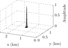
Figure 1: Illustration of the source shape for a localized boundary source.

The model (assimilated to a wavespeed here) is defined on a cubical (structured) domain partition of a rectangular block. With increasing $N$, the size of the cubes decreases, possibly non uniformly. We use piecewise constant functions on the cubes to define the wavespeeds following the main assumption for the Lipschitz stability to hold. Such a partition can be related to Haar wavelets, where $N$ determines the scale. These naturally introduce approximate representations, that is, when the scale of the approximation is coarser than the finest scale contained in the model.

In order to solve the forward problem, the numerical discretization of the operator is realized using discontinuous Galerkin method, where Dirichlet boundary conditions are invoked. The Dirichlet sources at the top boundary introduce Identity block in the discretized Helmholtz operator and give the following linear problem

(44) $$\left(\begin{matrix}A_{ii}&A_{i\partial}\\ A_{\partial i}&A_{\partial\partial}\end{matrix}\right)\left(\begin{matrix}u_{i}\\ u_{\partial}\end{matrix}\right)=\left(\begin{matrix}A_{ii}&A_{i\partial}\\ 0&Id\end{matrix}\right)\left(\begin{matrix}u_{i}\\ u_{\partial}\end{matrix}\right)=\left(\begin{matrix}0\\ g\end{matrix}\right),$$

where $A$ represents the discretized operator, $i$ labels interior points and $\partial$ labels boundary points, $g$ has values at the source location and is zero elsewhere. This system verifies $u_{\partial}=u_{|\partial\Omega}=g$ (i.e. Dirichlet boundary condition) and $A_{ii}u_{i}+A_{i\partial}u_{|\partial\Omega}=0$. The normal derivative data are generated by taking the normal derivative of the solution wavefield $u$ on the surface.

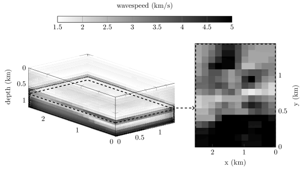
(a) Partition using $N=2,880$ domains.

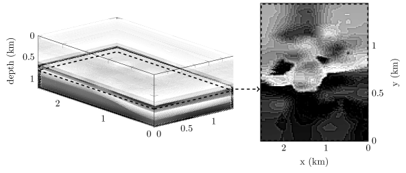
(b) Partition using $N=1,527,168$ domains.

Figure 2: Three dimensional representations and horizontal sections at $800$m depth of the reference wavespeed ($c_{1}$) using different partition, i.e. scales. Every scale has a structured (rectangular) decomposition using piecewise constant. The size of the rectangular boxes defines the scale of the wavespeed.

Our experiments use a three dimensional model of size $2.55\times 1.45\times 1.22$km. The wavesepeed $c_{1}$ is viewed as a reference model (which is known in this test case) and is represented Fig. 2 (courtesy Statoil). We also illustrate the different partitions of a model and the notion of approximation. Obviously the larger the number of subdomains is, the more precise will the representation be.

For the computation of the stability estimates we consider $c_{2}$ as the model shown in Fig. 3. This setup can be associated with the ‘true’ subsurface Fig. 2 and starting model Fig. 3. In this context we have chosen the initial guess with no knowledge of any structures by simply considering a one dimensional variation in depth.

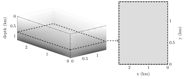
Figure 3: Three dimensional wavespeed used for the successive estimation of the stability constant ($c_{2}$), $3$D representation (left) and horizontal sections at $800$m depth (right).

3.1 Estimates using the full Dirichlet-to-Neumann map

We consider the full data case where the Gaussian sources (see Fig. 1) are positioned on each surface following a regular map. For each source, the data are acquired all over the boundary. We introduce a total of $630$ sources and $76538$ data points for each.

At a selected partition (number of domains) and frequency, we simulate the data for the two media $c_{1}$ and $c_{2}$ and compute the difference, from which we deduce the stability constant following equation Eq. 43.The main difference with the standard seismic setup is that we consider data on all the boundary and not only at the top. This last case will be mentioned in the Section 3.2.

The numerical estimates for the stability constant $\mathcal{C}$ should depend on the number of domains $N$ following the expression of the lower and upper bounds defined in the Remark 2.17, equations Eq. 39 and Eq. 41. Thus we fix the frequency and estimate the stability for different partitions. The evolution of the estimates and underlying bounds are presented in Fig. 4 at two selected frequencies, $5$ and $10$Hz. We plot on a $\log\log$ scale the function $\log(\mathcal{C}\omega^{2})$ to focus on the power of $N$ in the estimates, which is the slope of the lines ($4/7$ for the upper bound and $1/5$ for the lower bound).

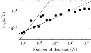
(a) Stability estimates at $5$Hz frequency

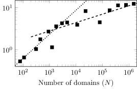
(b) Stability estimates at $10$Hz frequency

Figure 4: The black squares represent the computational estimates of the stability constant ($\blacksquare$) depending on the number of domains $N$ at selected frequency. The dashed line ($\boldsymbol{-}\boldsymbol{-}$) represents the analytical lower bound and the dotted line ($\boldsymbol{\cdot}\boldsymbol{\cdot}$) the upper bound, estimated with equation Eq. 45.

Regarding the different coefficients in the analytical bounds, $K$ and $K_{1}$ remain undecided and are numerically approximated so that the bounds match the estimates at best. For instance the numerical value for $K_{1}$ is obtained from equation (Eq. 39) by computing the average value based on the numerical stability estimates and $K$ is approximated following the same principle:

(45) $$K_{1}=\dfrac{1}{n_{st}}\sum_{i=1}^{n_{st}}\dfrac{\log(4\omega^{2}\mathcal{C}_{i})}{N_{i}^{1/5}},\quad\quad\quad\quad K=\dfrac{1}{n_{st}}\sum_{i=1}^{n_{st}}\dfrac{\log(\omega^{2}\mathcal{C}_{i})}{(1+\omega^{2}B_{2})N_{i}^{4/7}}.$$

Here, $n_{st}$ is the number of numerical stability constant estimates and $\mathcal{C}_{i}$ the corresponding estimate for partitioning $N_{i}$. We actually limit the computation of $K$ to use the first scales as it grows too rapidly. The numerical values obtained are given Table 1. We also note that the term $\omega^{2}B_{2}$ of the upper bound equation Eq. 41 is relatively small in the geophysical context as we have here $B_{2}=5.10^{-7}$.

We can see that the stability constant increases with the number of subdomains, as expected. There are clearly two states in the evolution of the estimates at the highest frequency (10Hz, 4(b)). For a low number of partitions $N$ the numerical estimates match particularly well the upper bound while at finer scale it follows accurately the lower bound. This is illustrated in Fig. 5 where we decompose the two parts of the estimates between the low and high number of domains.

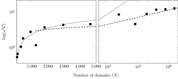
Figure 5: The black squares represent the computational estimates of the stability constant (LABEL:plot:mark_estimates_N) depending on the number of domains $N$ at $10$Hz. The left part shows the coarsest scales which match accurately the upper bound (dotted line, LABEL:plot:upper_bound). On the right the finer scale estimates are accurately anticipated by the lower bound (dashed line, LABEL:plot:lower_bound). The constants $K$ and $K_{1}$ for the computation of the lower and upper bounds are numerically approximated with values given Table 1, following equation Eq. 45.

Table 1: Numerical estimation of the constant in the analytical bounds formulation for the numerical estimates of the stability (Fig. 4), with $B_{2}=(1/1400)^{2}$).

	5Hz	10Hz
$K_{1}$	$1$	$0.7$
$K$	$0.15$	$0.05$

Alternatively for a lower frequency, i.e. $5$Hz on 4(a), the upper bound appears to increase too rapidly while the lower bound matches accurately the evolution of the stability constant estimates. Hence the upper bound we have obtained here is particularly appropriate for coarse scale and high frequency: when the variation of model is much coarser compared to the wavelength.

3.2 Seismic inverse problem using partial data

In realistic geophysical experiments for the reconstruction of subsurface area (seismic tomography), it is more appropriate not to consider the full data but partial data only located on the upper surface. The data obtain from $c_{1}$ can be seen as field observation (sensor measurement of a seismic event at the surface). The data using $c_{2}$ are simulation using an ‘initial guess’. For the reconstruction, we mention the full waveform inversion method, where the recovery follows an iterative minimization of the difference between the measurements and simulations, to successively update the initial guess (see [23, 20]). There is also the difference in the boundary conditions where perfectly matched layers (PMLs) or absorbing boundary conditions are invoked instead of the Dirichlet boundary condition for the lateral and bottom boundaries. However the top boundary is a free surface and remains a Dirichlet boundary condition.

For this test case we reproduce the same experiments but limiting the set of sources and the collected data to be at the top boundary only. We define a set of sources at the surface, separated by $160$m along the $x-$axis and $150$m along $y-$axis to generate a regular map of $16\times 10$ points. The receivers (data location) are positioned in the same fashion every $60$m along the $x-$axis and $45$m along $y-$axis and generate a regular map of $43\times 32$ points, see 6(a) and 6(b). The partial boundary data computed are illustrated for a single centered boundary shot at $5$Hz frequency 6(c).

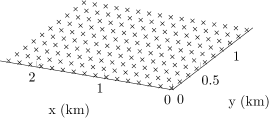
(a) the crosses represent the boundary sources locations.

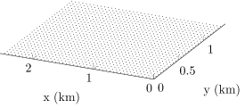
(b) The lattice represents the discretization of the data, i.e. the receivers location.

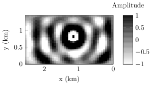
(c) Data recovered from a boundary centered shot, i.e. wavefield measured at the receivers location.

Figure 6: Illustration of the seismic acquisition set.

In Fig. 7 we compare the stability constant estimates using partial data with the stability constant estimates obtained when considering the full Dirichlet-to-Neumann map as the data. We incorporate the analytical lower bound that was computed in the previous test case.

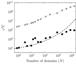
(a) Stability estimates at $5$Hz frequency

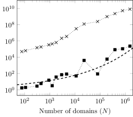
(b) Stability estimates at $10$Hz frequency

Figure 7: Comparison of the computational stability estimates using partial data only located on the top boundary ($\times$) and using the full boundary data ($\blacksquare$). The dashed line ($\boldsymbol{-}\boldsymbol{-}$) represents the analytical lower bound as found in Fig. 4.

The numerical estimates of the stability constants for the full and partial data in a $\log\log$-scale differ by a constant. This leads us to our conjecture that the $\log\log$ of the stability constants (as a function of $N$) of the full and partial data case in the continuous setting differ by a constant.

References

- [1] G. Alessandrini, Stable determination of conductivity by boundary measurements, Appl. Anal., 27 (1988), pp. 153–172, doi:10.1080/00036818808839730, http://dx.doi.org/10.1080/00036818808839730.
- [2] G. Alessandrini and S. Vessella, Lipschitz stability for the inverse conductivity problem, Adv. in Appl. Math., 35 (2005), pp. 207–241, doi:10.1016/j.aam.2004.12.002, http://dx.doi.org/10.1016/j.aam.2004.12.002.
- [3] G. Bao and P. Li, Inverse medium scattering problems for electromagnetic waves, SIAM J. Appl. Math., 65 (2005), pp. 2049–2066 (electronic), doi:10.1137/040607435, http://dx.doi.org/10.1137/040607435.
- [4] G. Bao and F. Triki, Error estimates for the recursive linearization of inverse medium problems, J. Comput. Math., 28 (2010), pp. 725–744, doi:10.4208/jcm.1003-m0004, http://dx.doi.org/10.4208/jcm.1003-m0004.
- [5] H. Ben-Hadj-Ali, S. Operto, and J. Virieux, Velocity model-building by 3d frequency-domain, full-waveform inversion of wide-aperture seismic data, Geophysics, 73 (2008), doi:10.1190/1.2957948.
- [6] E. Beretta, M. V. de Hoop, and L. Qiu, Lipschitz stability of an inverse boundary value problem for a Schrödinger-type equation, SIAM J. Math. Anal., 45 (2013), pp. 679–699, doi:10.1137/120869201, http://dx.doi.org/10.1137/120869201.
- [7] E. Beretta and E. Francini, Lipschitz stability for the electrical impedance tomography problem: the complex case, Comm. Partial Differential Equations, 36 (2011), pp. 1723–1749, doi:10.1080/03605302.2011.552930, http://dx.doi.org/10.1080/03605302.2011.552930.
- [8] K. D. Blazek, C. Stolk, and W. W. Symes, A mathematical framework for inverse wave problems in heterogeneous media, Inverse Problems, 29 (2013), p. 065001.
- [9] K. Datchev and M. V. de Hoop, Iterative reconstruction of the wavespeed for the wave equation with bounded frequency boundary data, arXiv preprint arXiv:1506.09014, (2015).
- [10] E. B. Davies, Spectral theory and differential operators, vol. 42 of Cambridge Studies in Advanced Mathematics, Cambridge University Press, Cambridge, 1995, doi:10.1017/CBO9780511623721, http://dx.doi.org/10.1017/CBO9780511623721.
- [11] J. Feldman, M. Salo, and G. Uhlmann, The Calderón problem — An Introduction to Inverse Problems, unpublished ed., 2015, http://www.math.ubc.ca/~feldman/ibook/.
- [12] D. Gilbarg and N. S. Trudinger, Elliptic partial differential equations of second order, vol. 224 of Grundlehren der Mathematischen Wissenschaften [Fundamental Principles of Mathematical Sciences], Springer-Verlag, Berlin, second ed., 1983.
- [13] P. Hähner, A periodic Faddeev-type solution operator, J. Differential Equations, 128 (1996), pp. 300–308, doi:10.1006/jdeq.1996.0096, http://dx.doi.org/10.1006/jdeq.1996.0096.
- [14] P. Hähner and T. Hohage, New stability estimates for the inverse acoustic inhomogeneous medium problem and applications, SIAM Journal on Mathematical Analysis, 33 (2001), pp. 670–685, doi:10.1137/S0036141001383564, http://dx.doi.org/10.1137/S0036141001383564, arXiv:http://dx.doi.org/10.1137/S0036141001383564.
- [15] T. Hohage, Logarithmic convergence rates of the iteratively regularized gauss - newton method for an inverse potential and an inverse scattering problem, Inverse Problems, 13 (1997), p. 1279, http://stacks.iop.org/0266-5611/13/i=5/a=012.
- [16] R. Magnanini and G. Papi, An inverse problem for the Helmholtz equation, Inverse Problems, 1 (1985), pp. 357–370, doi:10.1088/0266-5611/1/4/007, http://dx.doi.org/10.1088/0266-5611/1/4/007.
- [17] N. Mandache, Exponential instability in an inverse problem for the Schrödinger equation, Inverse Problems, 17 (2001), pp. 1435–1444, doi:10.1088/0266-5611/17/5/313, http://dx.doi.org/10.1088/0266-5611/17/5/313.
- [18] S. Nagayasu, G. Uhlmann, and J.-N. Wang, Increasing stability in an inverse problem for the acoustic equation, Inverse Problems, 29 (2013), p. 025012, doi:10.1088/0266-5611/29/2/025012, http://dx.doi.org/10.1088/0266-5611/29/2/025012.
- [19] R. G. Novikov, New global stability estimates for the Gel’fand-Calderon inverse problem, Inverse Problems, 27 (2011), p. 015001, doi:10.1088/0266-5611/27/1/015001, http://dx.doi.org/10.1088/0266-5611/27/1/015001.
- [20] R. G. Pratt, C. Shin, and G. J. Hicks, Gauss-newton and full newton methods in frequency-space seismic waveform inversion, Geophysical Journal International, 133 (1998), pp. 341–362.
- [21] J. Sylvester and G. Uhlmann, A global uniqueness theorem for an inverse boundary value problem, Ann. of Math. (2), 125 (1987), pp. 153–169, doi:10.2307/1971291, http://dx.doi.org/10.2307/1971291.
- [22] W. W. Symes, The seismic reflection inverse problem, Inverse Problems, 25 (2009), pp. 123008, 39, doi:10.1088/0266-5611/25/12/123008, http://dx.doi.org/10.1088/0266-5611/25/12/123008.
- [23] A. Tarantola, Inversion of seismic reflection data in the acoustic approximation, Geophysics, 49 (1984), pp. 1259–1266.