A study of spatial correlations in pulsar timing array data

Abstract

Pulsar timing array experiments search for phenomena that produce angular correlations in the arrival times of signals from millisecond pulsars. The primary goal is to detect an isotropic and stochastic gravitational wave background. We use simulated data to show that this search can be affected by the presence of other spatially correlated noise, such as errors in the reference time standard, errors in the planetary ephemeris, the solar wind and instrumentation issues. All these effects can induce significant false detections of gravitational waves. We test mitigation routines to account for clock errors, ephemeris errors and the solar wind. We demonstrate that it is non-trivial to find an effective mitigation routine for the planetary ephemeris and emphasise that other spatially correlated signals may be present in the data.

1 Introduction

The pulsar timing method provides a way to study the physics and astrometry of individual pulsars, the properties of the intervening interstellar medium and to search for un-modeled phenomena. Pulsar times-of-arrival (ToAs) are first measured at radio observatories and then converted to the reference frame of the solar-system barycenter (SSB). The extreme rotational stability of pulsars enable these barycentric ToAs to be predicted using a simple model (known as the “pulsar ephemeris”) for the pulsar’s rotational and orbital motion. Differences between the measured and predicted ToAs are referred to as “timing residuals”. Features in the timing residuals (which imply a temporal correlation between the ToAs of an individual pulsar) indicate that the model with which we are describing the pulsar is not complete. It may not account for some events, such as glitches (e.g., Wang et al. 2012), variations in the interstellar medium (e.g., Keith et al. 2013) or intrinsic instabilities in the pulsar rotation (e.g., Shannon & Cordes 2010). The power spectrum of such residuals is often “red”, that is, characterized by an excess of power at lower fluctuation frequencies. In contrast, “white” power spectra have statistically the same amount of power for each frequency. An iterative process is followed to improve the pulsar model in order to minimize the residuals. Numerous studies have already been carried out using this technique, including tests of theories of gravity (e.g., Kramer et al. 2006), analyses of the Galactic pulsar population (e.g., Lorimer et al. 2006) and the interstellar medium (e.g., Keith et al. 2013).

Pulsar Timing Array (PTA) projects are employing this technique to study phenomena that simultaneously affect multiple pulsars. A main goal of PTA experiments is the direct detection of an isotropic and stochastic gravitational wave background (GWB; e.g., Hellings & Downs 1983) generated by the superposition of the gravitational-wave emission of coalescing super-massive black-hole binaries (Sesana, 2013a). Other noise processes that simultaneously affect many pulsars are, for example, irregularities in terrestrial time standards (Hobbs et al., 2012) and poorly determined solar system ephemerides (Champion et al., 2010).

In all of the cases mentioned above, the pulsar ToAs will be spatially and temporally correlated. PTA projects seek to measure the spatial correlation $C(\theta_{ij})$ between a pair of pulsars (labeled $i$ and $j$) separated by an angle $\theta_{ij}$. The $C(\theta_{ij})$ coefficients are analyzed to identify the physical phenomenon that leads to the correlation. In particular, a GWB would induce a specific shape in the spatial correlations (see Figure 1), called the “Hellings and Downs curve” (Hellings & Downs, 1983). If the Hellings and Downs curve is significantly detected, then a GWB detection will be claimed.

To date, no GWB detection has been made. Because the first direct detection of GWs will be of enormous astrophysical interest, the chance of false detections must be well understood. After a detection, the first step will be to determine an unbiased estimate of the properties of that background (such as its amplitude). It is therefore fundamental to verify whether any other physical effects could lead to an angular correlation whose cause could be misidentified as a GWB.

In this paper, we study the impact of various noise processes that would correlate between different pulsars on the GWB search in PTA data. In particular, we study simplified versions of the signals that we expect from realistic errors in the clock time standard and in the planetary ephemeris. We also discuss a set of mitigation routines to remove the effect of these noise processes before providing an estimate of real errors in the clock and planetary ephemeris. We consider other possible correlated noise processes that might be hidden in the data.

To carry out our research, we use simulated data sets. In Section 2 we outline the properties of the noise processes that we simulate. In Section 3 we describe how we realize these simulations and their processing. In Section 4 we present and discuss our results, and draw our conclusions in Section 5.

2 Correlated signals in pulsar data

PTA pulsars are generally widely separated ($\gg 1$ degree) on the sky. Noise induced by the interstellar medium and the intrinsic timing noise (unexplained low-frequency noise in the timing residuals of a single pulsar) of each individual pulsar is expected to be uncorrelated between pulsar pairs:

$$C(\theta_{\rm ij})=0.$$ (1)

Pulse ToAs are referred to an observatory time standard. However, observatory clocks are not perfect and so the ToAs are converted to a realization of Terrestrial Time (TT). This conversion is carried out with a precision usually better than $\sim$1 ns; see Hobbs et al. (2012). Two main realizations of TT are commonly used. Terrestrial Time as realized by International Atomic Time (TAI) is a quasi-real-time time standard. This is subsequently updated to produce the world’s best atomic time standard, the Terrestrial Time as realized by the Bureau International des Poids et Mesures (BIPM). Any errors in the Terrestrial Time standard will induce the same timing residuals in all pulsars:

$$C(\theta_{\rm ij})=1,$$ (2)

or, the correlation between pulsars affected by an error in the clock time standard is monopolar.

The pulsar timing procedure also relies upon knowledge of the position of the SSB with respect to the observatory. The position of the observatory with respect to the center of the Earth is usually precisely known. In this case, we only need to consider possible errors in the solar system ephemeris used to convert pulse ToAs from the Earth’s center to the SSB. The Jet Propulsion Laboratory (JPL) series of ephemerides are often used for this conversion. In this paper we make use of the ephemerides DE414 and DE421. The effect of an error in the planetary ephemeris on the pulsar timing residuals, $r$, is:

$$r_{\rm i}(t)=\frac{1}{c}{\bf e}(t)\cdot{\bf\hat{k}}_{\rm i}$$ (3)

where $c$ is the vacuum speed of light, ${\bf e}$ is the time-dependent error in position of the SSB with respect to the observatory and ${\bf\hat{k}}_{\rm i}$ is a unit vector pointed toward pulsar $i$. Instantaneously, this is a dipolar effect. If the vector ${\bf e}$ is sufficiently independent of the ${\bf\hat{k}}_{\rm i}$ and ${\bf\hat{k}}_{\rm j}$ vectors, (as discussed in Appendix A) then the $C(\theta_{ij})$ would assume a $\cos(\theta_{ij})$ angular dependence.

The ToA delays induced by the passage of a GW includes the effect of the GW passing the pulsar (often known as the “pulsar term”) and also the effect of the GW passing the Earth (the “Earth term”). Recent work (Sesana et al., 2009; Ravi et al., 2015) suggests that the most likely detectable signal will be a stochastic and isotropic background of GWs (GWB) caused by a large number of supermassive, binary black-hole systems. The “pulsar term” will lead to red, uncorrelated noise in the pulsar timing residuals. Hellings & Downs (1983) showed that the correlations induced by the “Earth term” would leave a well-defined signature in the angular correlation between the timing residuals of different pulsars. The signature, known as the “Hellings & Downs curve”, is shown as the continuous line in Figure 1 and is defined by:

$$C(\theta_{\rm ij})=\frac{3}{2}x\log(x)-\frac{x}{4}+\frac{1}{2}$$ (4)

where $x=[1-\cos(\theta_{\rm ij})]/2$. The power spectrum for a GWB may be described by a power law:

$$P_{\rm GWB}(f)=\frac{\rm A^{2}}{12\pi^{2}}\left(\frac{f}{f_{\mathrm{yr}}}\right)^{2\alpha-3}$$ (5)

where A is the GWB amplitude for a frequency $f=f_{\mathrm{yr}}=(1\mathrm{yr})^{-1}$, $\alpha$ sets the power-law slope, which is predicted to be $-2/3$ for an isotropic and stochastic GWB (Phinney, 2001). Current upper bounds on the amplitude of the GWB indicate that A is smaller than 10^-15 (Shannon et al., submitted).

The search for the GWB is based on determining the correlation between the timing residuals for each pair of pulsars in a given PTA. The subsequent steps of the search depend on the adopted statistical approach. The PPTA have generally made us of a frequentist method (e.g., Yardley et al. 2011, hereafter Y11) to determine whether or not the correlations take the form of the Hellings & Downs curve. If they do, then a detection of the GWB will be claimed. We note that this functional form will never be perfectly matched in practice. First, the Hellings & Downs curve is not obtained through independent measurements of the angular covariance. For a given PTA, only a finite number of pulsar pairs exists and the measured correlations will not be independent as a given pulsar will contribute to multiple pairs. The Hellings & Downs curve is an ensemble average. For our Universe, the positions and properties of the black-hole binaries along with the effect of the GWB passing each pulsar will lead to noise on the expected curve (see e.g., Ravi et al. 2012). Various algorithms, both frequentist and Bayesian, have been developed to search for the signature of the Hellings & Downs curve (Yardley et al., 2011; van Haasteren et al., 2011; Demorest et al., 2013; Lentati et al., 2015) and have been applied to actual data sets.

If a non-GWB noise process that produces spatially correlated timing residuals is well understood then it will be possible to develop mitigation routines or to include such noise as part of GWB detection algorithms. We have already considered two signals (clock and ephemeris errors) that are extensively discussed by PTA research teams, but note that many other such processes may be present. These include instrumental artifacts, solar wind effects, polarization calibration errors, uncertainties in the Earth-orientation-parameters, the ionosphere, the troposphere, individual gravitational wave sources and many other possibilities. For this paper, we have chosen to study instrumental delays and the solar wind as representative examples.

The configuration of the observational set-up for receivers and signal-processing systems is optimized on the basis of the pulse period and dispersion measure (DM) for each pulsar. Therefore, it may be that different pulsars are characterized by different observational set-ups. For all PTAs, both receivers and signal-processing systems have evolved over the data spans (see, e.g., Manchester et al. 2013 for details). Such updates can introduce time offsets into the timing residuals that are dependent upon the specific configuration used. Although PTA teams attempt to compute them, these measurements have an uncertainty, and thus some small offsets remain. Therefore, the pulsar data sets may include an offset that is identical for pulsar pairs with the same observational configuration, but has a different amplitude for pulsar pairs with different set-ups.

Fluctuations in the plasma density of the solar wind and the ionosphere will cause correlated noise in the timing residuals of different pulsars if the DM corrections are not made on a sufficiently fine time scale. As the the solar wind variations yield the most severe impact between these two effects, we have included them in our simulations. The solar wind variations depend on the angular distance between the pulsar and the Sun and the solar latitude of the point where the line of sight is closest to the Sun (You et al., 2007). The size of this effect will change during the solar cycle (see e.g., You et al. 2012). The tempo2 software attempts to account for the solar wind using a non-time-dependent and spherically symmetric model (see e.g., Edwards et al. 2006). It is often assumed that any remnant signal could be absorbed into standard measurements of DM variations for each pulsar. However, variations in the solar wind may occur on time scales faster than the typical smoothing time for dispersion measure correction (see e.g., Keith et al. 2013), or be in disagreement with some proposed models for DM fluctuations (e.g., Lee et al. 2014).

3 Method

Table 1: Some parameters of the PPTA pulsar sample simulated in this study.

PSR name	Spin period	RA	Dec	Ecliptic latitude
	[ms]	[hh:mm:ss]	[dd:mm:ss]	[deg]
J0437$-$4715	5.757	04:37:15.8	$-$47:15:08.6	$-$67.9
J0613$-$0200	3.062	06:13:43.9	$-$02:00:47.1	$-$25.4
J0711$-$6830	5.491	07:11:54.2	$-$68:30:47.5	$-$82.9
J1022+1001	16.453	10:22:58.0	+10:01:53.2	$-$0.1
J1024$-$0719	5.162	10:24:38.6	$-$07:19:19.1	$-$16.0
J1045$-$4509	7.474	10:45:50.1	$-$45:09:54.1	$-$47.7
J1600$-$3053	3.598	16:00:51.9	$-$30:53:49.3	$-$10.1
J1603$-$7202	14.842	16:03:35.6	$-$72:02:32.7	$-$50.0
J1643$-$1224	4.622	16:43:38.1	$-$12:24:58.7	+9.8
J1713+0747	4.57	17:13:49.5	+07:47:37.5	+30.7
J1730$-$2304	8.123	17:30:21.6	$-$23:04:31.2	+0.2
J1732$-$5049	5.313	17:32:47.7	$-$50:49:00.1	$-$27.5
J1744$-$1134	4.075	17:44:29.4	$-$11:34:54.6	+11.8
J1857+0943	5.362	18:57:36.3	+09:43:17.3	+32.3
J1909$-$3744	2.947	19:09:47.4	$-$37:44:14.3	$-$15.2
J1939+2134	1.558	19:39:38.5	+21:34:59.1	+42.3
J2124$-$3358	4.931	21:24:43.8	$-$33:58:44.6	$-$17.8
J2129$-$5721	3.726	21:29:22.7	$-$57:21:14.1	$-$39.9
J2145$-$0750	16.052	21:45:50.4	$-$07:50:18.4	+5.3
J2241$-$5236	2.187	22:41:42.0	$-$52:36:36.2	$-$40.4

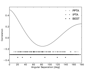
Figure 1: The continuous line represents the expected Hellings & Downs curve. Crosses, dots and stars show the angular coverage offered by, respectively, the PPTA pulsars, the IPTA pulsars (see Table 1) and the four best PPTA (and IPTA) pulsars: PSRs J0437$-$4715, J1713+0747, J1744$-$1134 and J1909$-$3744.

In order to study the effect of correlated noise processes on the GWB search in PTA data we 1) simulate data sets in which we artificially inject signals that might induce spatial correlations between pulsar time series and 2) process each simulation as if only a GWB was present in the data. PTA data sets are subject to various complexities: different pulsars may have different data spans, the precision with which the ToAs can be determined is affected by the flux density of the pulsar and interstellar scintillation and the observational sampling is non-uniform.

In this paper, we have chosen to simulate much simpler (albeit unrealistic) data sets, with regular sampling and equal uncertainties and data spans. With such data sets, our software is faster and many of the results can be understood analytically. We also note that if an analysis of these data sets can lead to misidentifications of a GWB, then the additional effects evident in actual data may provide an even higher chance of false detections.

We simulate data sets for 20 of the millisecond pulsars (MSPs) observed by the PPTA (listed in Table 1). The coverage of the Hellings & Downs curve offered by these pulsars is shown by the cross symbols in Figure 1. We note that the closest pulsar pair is PSR J2129$-$5721 - PSR J2241$-$5236 with an angular distance of $11.36$ degrees, and the most widely separated is PSR J1022$+$1001 - PSR J2145$-$0750 with an angular distance of $170.57$ degrees. Only nine pulsar pairs have angular separations wider than $140$ degrees. The angular coverage given by the four most precise timers of the three PTAs (J0437$-$4715, J1713$+$0747, J1744$-$1134 and J1909$-$3744) is also shown in Figure 1 (star symbols), and ranges from 20 to 140 degrees.

We simulate the ToAs using the ptaSimulate software package. This software is based on the simulation routines developed for tempo2. Initially, the software simulates the observing times. In our case, we simply assume that each of the 20 PPTA pulsars are observed from MJD 48000 to 53000 (a span of 5000 days, 13.7 years), with a cadence of 14 days. The software then uses the deterministic pulsar timing models (obtained from the ATNF Pulsar Catalogue) for each of the pulsars to form idealized site arrival times based on the observation times (see Hobbs et al. 2009 for details). These timing models are referred to the JPL ephemeris DE421 and the time standard TT(BIPM2013). Later, the software creates 1000 realizations of the various noise processes, which we add to the arrival times together with 100 ns of white Gaussian noise to represent the radiometer noise level.

We first simulate 1000 realizations of time series affected by an isotropic, stochastic GWB, S_gwb with an amplitude of 10^-15. This was achieved by assuming 1000 individual GW sources isotropically distributed on the sky with amplitudes and frequencies chosen such that the resulting power spectrum of the background is consistent with Equation 5 (Hobbs et al., 2009). S_gwb is our reference simulation throughout this paper.

We then study the likelihood that each specific noise process can be mis-identified as a GWB, by individually adding these signals to the simulated arrival times described above. We do not know the exact levels, nor the spectral shapes that such signals will assume in real data sets. For this reason, we choose the following approach. We first determine whether noise processes with the same spectrum and amplitude of the GWB in S_gwb can lead to false detections. The red noise processes given below were therefore all simulated to have spectra consistent with that of a GWB with an amplitude A = 10^-15:

• S_utn, spatially uncorrelated timing noise. A scaling factor, which converts the real and imaginary parts of a Fourier transform to the required power spectrum, is determined. The real and imaginary parts are randomized by multiplying by a Gaussian random value. The corresponding time series is obtained by carrying out a complex-to-real Fourier transform;

• S_clk, stochastic, monopolar clock-like signal. Its characteristics are based on our expectation of an error in the clock time standard. For each realization, we derive a single time series as for S_utn and assume that this noise process affects all the pulsars;

• S_eph, stochastic, dipolar ephemeris-like signal. Its characteristics are based on our expectation of an error in the planetary ephemeris. For each realization, we simulate three time series as for S_utn. We assume that these three time series represent the time series of errors in the three spatial components of ${\bf e}$. The timing residuals for a given pulsar are then obtained using Equation 3.

We also simulate other four noise processes that are not at the same level nor have the same spectral shape as the simulated GWB:

• S_tt, we simulate time series based on the TT(BIPM2013), and we then process the time series by using TT(TAI). We thus simulate the effects of a clock error corresponding to the difference between TT(BIPM2013) and TT(TAI);

• S_de, we simulate time series based on the DE421, and we then process the time series by using DE414. We thus simulate the effects of an ephemeris error corresponding to the difference between DE421 and DE414;

• S_ie, we divide the pulsars of our sample in three groups (consisting of 7, 7 and 6 pulsars respectively). We assume that each group was observed with a different signal-processing system. We assume that the systems are modified six times over the total data span. This introduces time delays in the ToAs. We assume that the epochs of the modifications are the same for the three systems, but that the amplitudes of the time offsets are different. We also assume that these offsets vary for the same signal-processing system from one epoch to the other. The amplitude of the offsets (for each epoch and system) was randomly drawn from a Gaussian population a standard deviation of 20 ns. We also test the effects for a standard deviation of 200 ns;

• S_sw, we include the expected effects of the solar wind by modeling the solar corona using observations from the Wilcox Solar Observatory when calculating the idealized site arrival times. This process is based on the procedure first described by You et al. (2007). We subsequently processed the pulsar observations assuming that the solar wind is absent.

These simulations are listed in Table 2. We note that the GWB simulations require knowledge of the pulsar distances. In our case, the code computes an approximate distance based on the DM measurement. We also note that S_tt, S_de and S_sw are all deterministic simulations, and that the only change between the 1000 iterations is the realization of the white noise for each pulsar.

Table 2: Summary of the simulations. All the simulations include 1000 iterations of the timing residuals of 20 pulsars with a white noise level of 100 ns, each spanning 5000 days and sampled at 14 day intervals. The simulations that assume a GWB spectrum have a spectral amplitude of 1$\times 10^{-15}$.

Tag	Simulated effect	GWB-like
		spectrum
Sgwb	GWB	Y
Sutn	Uncorrelated red noise	Y
Sclk	Stochastic clock-like errors	Y
Seph	Stochastic ephemeris-like errors	Y
Stt	Difference between TT(BIPM2013) and TT(TAI)	N
Sde	Difference between DE421 and DE414	N
Sie	Instrumental errors	N
Ssw	Solar wind	N

3.1 Simulation processing and computation of the angular covariance

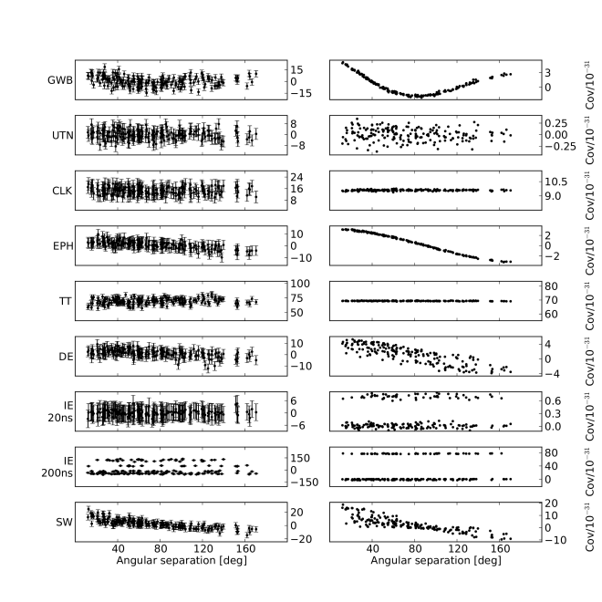
Figure 2: Angular covariances computed the simulations described in Section 3. From top to bottom: S_gwb, S_utn, S_clk, S_eph, S_tt, S_de, S_ie at 20 ns, S_ie at 200 ns, S_sw. In the left panels is shown the result for an individual realization, in the right panels is shown the average over 1000 realizations.

Our simulation software provides a set of pulsar timing models and arrival time files that can be processed in an identical manner to actual pulsar data. These timing models have already been fitted for changes in the pulse frequency and its time derivative for each pulsar (and, in the case of S_de, we also fit for the pulsar position). We wish to extract from these simulated data sets the correlated noise that could lead to a false detection of a GWB. Numerous GWB detection codes exist (Yardley et al., 2011; van Haasteren et al., 2011; Demorest et al., 2013; Lentati et al., 2015). We chose to use an updated version of the algorithms developed by Y11 because 1) it has been implemented in the tempo2 public plugin detectGWB, 2) the code runs quickly, 3) it produces a large amount of useful diagnostic output and 4) it is easy for us to implement the mitigation methods that we describe below. The Y11 code first calculates the covariances between the timing residuals for each pulsar pair. It then obtains a value for the squared GWB amplitude, $\hat{\rm A}^{2}$, by fitting the Hellings & Downs curve to these covariance estimates. We therefore obtain an estimate of the GWB amplitude for each of our 1000 realizations.

We have updated the Y11 algorithm as follows. We linearly interpolate a grid of uniformly spaced values onto the pulsar timing residuals. The obtained grid of values is constrained so that the corresponding rotational frequency and its derivative are zero. We then select the grid points that are in common between a given pulsar pair and form cross power spectra using a red noise model and the Cholesky fitting routines (see Coles et al. 2011). This allows us to calculate power spectra in the presence of steep red noise. The noise model that we assume throughout is given by Equation 5 with A = 10^-15. The Y11 algorithm also requires an initial guess for the GWB amplitude. For this guess we also chose A = 10^-15. This implies that the algorithm will be optimal for the case in which the GWB is present and allows us to evaluate the occurrence of false detections in the other data sets.

The output from the Y11 algorithm includes both an evaluation of A² ($\hat{\rm A}^{2}$), a 1-$\sigma$ error bar on this measurement ($\sigma_{\hat{\rm A}^{2}}$) and the significance of the detection (defined as $\hat{\rm A}^{2}/\sigma_{\hat{\rm A}^{2}}$). As our statistic, we chose to use $\hat{\rm A}^{2}$ because it provides an unbiased estimator for the power in the timing residuals that can be attributed to a GWB. All our modifications are available in the most recent release of the detectGWB plugin.

We applied our method to all realizations of all our simulations. In Figure 2 we show the covariances obtained as a function of the angle between each pulsar pair. In the left-hand column we show an individual realization for each noise process. In the right-hand column we show the covariances after averaging over the 1000 realizations. In the next section we discuss each of these noise processes in detail.

4 Results and discussion

We calculated the distribution of $\hat{\rm A}^{2}$ values from each of the 1000 realizations of every simulated noise process. In Table 3 we list the corresponding mean and standard deviation of the distribution. For the simulations that do not include a GWB, we also determine the $\hat{\rm A}^{2}$ value that is exceeded in only 5% of the simulations. This value (“DT5”) represents the detection threshold that would have a 5% false alarm probability. We also determine how many realizations of S_gwb exceed this threshold (P_DT5), i.e. the probability of detection at this threshold. In other words, DT5 represents the correct detection threshold for the analyzed type of noise, while P_DT5 is the probability of detection if the GWB amplitude is 1$\times 10^{-15}$ and we assume DT5 as the actual detection threshold. We trial various mitigation methods to reduce DT5 and thus increase P_DT5. These mitigation methods are described in detail below and the corresponding results are also listed in Table 3. For these results we apply the same mitigation routine to S_gwb as we have applied to the simulation being processed.

Table 3: Summary of the simulation results. In the columns are indicated, respectively, the simulation name, the applied mitigation routine, mean $\hat{\rm A}^{2}$, standard deviation of the $\hat{\rm A}^{2}$ distribution, DT5 and P_DT5. The mean, standard deviation and DT5 values are given with respect to 10^-30

Simulation	Mitigation routine	Mean	Standard deviation	DT5	PDT5
Sgwb	$-$	1.2	0.53	$-$	$-$
	Clock: offset subtraction	1.2	0.53	$-$	$-$
	Clock: Hobbs et al. 2012	0.98	0.43	$-$	$-$
	Ephemeris: cosine subtraction	1.2	0.53	$-$	$-$
	Ephemeris: Deng et al. 2013	0.40	0.24	$-$	$-$
	Ephemeris: Champion et al. 2010	0.88	0.40	$-$	$-$
Sutn	$-$	0.0050	0.18	0.32	98 %
Sclk	$-$	0.68	0.36	1.3	33 %
	Clock: offset subtraction	$-$0.0066	0.14	0.25	99 %
	Clock: Hobbs et al. 2012	0.0043	0.052	0.089	99 %
Seph	$-$	0.36	0.19	0.74	81 %
	Ephemeris: cosine subtraction	$-$0.00019	0.12	0.20	99 %
	Ephemeris: Deng et al. 2013	$-$0.021	0.034	0.041	97 %
	Ephemeris: Champion et al. 2010	0.090	0.13	0.31	95 %
Stt	$-$	4.9	0.33	5.5	0 %
	Clock: offset subtraction	$-$0.00067	0.31	0.0053	93 %
	Clock: Hobbs et al. 2012	0.0040	0.053	0.097	99 %
Sde	$-$	0.44	0.14	0.68	86 %
	Ephemeris: cosine subtraction	0.0029	0.14	0.25	99 %
	Ephemeris: Deng et al. 2013	$-$0.024	0.12	0.18	83 %
	Ephemeris: Champion et al. 2010	0.025	0.13	0.25	97 %
Sie (20 ns)	$-$	$-$0.0021	0.069	0.11	99 %
Sie (200 ns)	$-$	$-$0.36	2.1	3.1	0 %
Ssw	$-$	1.6	0.14	1.8	11 %
	Solar wind: tempo2 model	0.43	0.12	0.64	$-$
	Solar wind: adaptation of Keith et al. 2013	1.2	0.061	1.3	$-$

4.1 GWB and uncorrelated timing noise

Figure 3 shows the $\hat{\rm A}^{2}$ distribution obtained for S_gwb (dotted histogram). The mean value, 1.2$\times 10^{-30}$, is slightly higher than the expected (1$\times 10^{-30}$). This is a known bias within the Y11 algorithm that occurs because the individual covariances are not independent. Y11 accounted for this bias by using simulations to determine a scaling factor. For our work this bias is small and does not affect our conclusions. The top panel in Figure 2 shows that we successfully recover the expected Hellings & Downs signature.

The solid-line histogram in Figure 3 shows the results from S_utn (uncorrelated noise process). As expected, the mean of this histogram (5$\times 10^{-33}$) and the corresponding angular covariances are statistically consistent with zero. The P_DT5 of this simulation indicates that the $\hat{\rm A}^{2}$ values obtained from 98% of the S_gwb simulations are above the detection threshold. It is therefore unlikely that, with a careful analysis of the angular correlations in Figure 2 and the false alarm probability, the S_utn simulations could be misidentified as a GWB.

4.2 Clock-like error

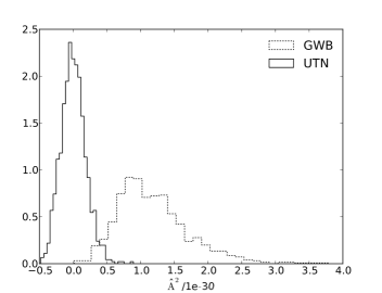
Figure 3: Normalized $\hat{\rm A}^{2}$ distributions obtained for simulations S_utn (solid) and S_gwb (dotted).

The top panel of Figure 4 contains the $\hat{\rm A}^{2}$ distribution obtained for S_clk, overlaid with the $\hat{\rm A}^{2}$ values computed for S_gwb. The two distributions significantly overlap. The Y11 algorithm produces non-zero $\hat{\rm A}^{2}$ values with a mean of 6.8$\times 10^{-31}$ and a DT5 of 1.3$\times 10^{-30}$. The P_DT5 is 33%. Blind use of a detection code can therefore lead to a false detection of a GWB in the presence of such a clock signal. However, the angular correlations for a clock error as a function of angular separation take the form of a constant offset (see Figure 2) and are easily distinguishable by eye from the Hellings & Downs curve. We can therefore update the GWB detection code to account for the possibility of clock errors.

We consider two general approaches: 1) we can mitigate the effects that the spurious signal has on the angular covariances or 2) we can identify and subtract the signal directly from the time series. In the first method, we note that the clock errors lead to an offset in the angular correlations. We can therefore attribute any offset to clock errors and update the detection algorithm to search for the Hellings & Downs curve with a mean removed. In the second method, we can first measure the clock errors from the timing data, subtract them from the residuals and then apply the detection algorithm.

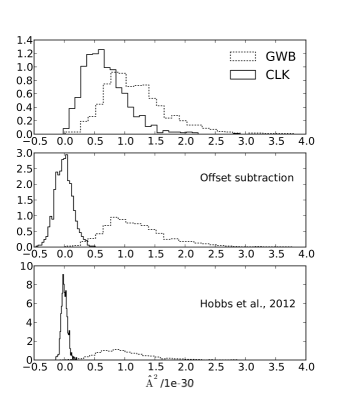
Figure 4: In the upper panel are shown the normalized $\hat{\rm A}^{2}$ distributions as computed for simulations S_clk (solid histograms) and S_gwb (dotted histogram). In the central and the bottom panels we show the same distributions, after the application of the two mitigation routines described in Section 4.2.

For the first case, we update the Y11 algorithm to include a constant offset, $\gamma$, when fitting for the $\hat{\rm A}^{2}$ values. i.e., we fit the following function to our measured covariances:

$$f(\theta_{ij})=\hat{\rm A}^{2}C(\theta_{ij})+\gamma.$$ (6)

The resulting $\hat{\rm A}^{2}$ distribution for S_clk and S_gwb after this modification is shown in the central panel of Figure 4 (respectively the solid and dotted histogram). The mean of the S_clk distribution is now statistically consistent with zero. The standard deviation of the distribution is reduced with respect to the non-mitigated results by a factor of $\sim 2.5$ and the DT5 is reduced by a factor of $\sim 5$. The application of this correction routine does not affect S_gwb.

In the second case, we determine and remove the clock signal before applying the GWB search algorithm (Hobbs et al., 2012). This procedure requires to search for a common signal in the time series, and it is carried out by simultaneously fitting all the timing residuals with an even grid of linearly interpolated values. We choose a regular sampling of 150 days, but note that the results do not significantly depend upon this choice.

As the mean of the Hellings & Downs curve is non-zero, the clock subtraction procedure will identify it as a clock signal and remove it. Therefore, the fit for $\hat{\rm A}^{2}$ performed by detectGWB needs to be updated to fit the measured covariances with the following function:

$$g(\theta_{ij})=\hat{\rm A}^{2}(C(\theta_{ij})-\langle C\rangle)$$ (7)

where $\langle C\rangle$ is the mean value of the Hellings & Downs curve computed on the angular separations determined by the pulsars in the sample. Our resulting $\hat{\rm A}^{2}$ distributions are shown in the bottom panel of Figure 4 for S_clk and S_gwb. We obtain a distribution mean that is consistent with zero for S_clk. The standard deviation and the DT5 decrease with respect to the non-mitigated simulations by factors of $\sim 7$ and $\sim 15$ respectively. Applying this correction routine to S_gwb, the mean of the $\hat{\rm A}^{2}$ distribution decreases by about 18%. It is statistically consistent with the average $\hat{\rm A}^{2}$ of the non mitigated simulations (see Table 3).

We therefore conclude that:

• Without correction, clock errors may yield large values of $\hat{\rm A}^{2}$ when searching for a GWB in PTA data sets, and hence false detections;

• It is possible to correct for clock errors without affecting the sensitivity to a GWB signal;

• To measure and remove the clock signal from the time series before searching for the GWB is a satisfactory mitigation method.

4.3 Ephemeris-like error

The $\hat{\rm A}^{2}$ values obtained for S_eph, without applying any of the clock correction routines discussed above, are shown in the top panel of Figure 5 (solid histogram) overlaid on the GWB values. The histograms partially overlap although the angular covariances shown in Figure 2 are clearly different.

As for the clock-like errors, we can 1) update the detection code to account for the signature left by ephemeris errors on the angular covariances or 2) we can first attempt to measure and remove the ephemeris errors from the pulsar time series.

In the first case, we update the Y11 detection algorithm to include a cosinusoidal function (see Appendix A) while fitting for $\hat{\rm A}^{2}$, i.e., we fit the following function to the measured covariances:

$$f(\theta_{ij})=\hat{\rm A}^{2}C(\theta_{ij})+\alpha\cos{\theta_{ij}}.$$ (8)

The resulting $\hat{\rm A}^{2}$ values are shown in the second panel of Figure 5, both for S_eph and S_gwb. The distribution mean for S_eph is now statistically consistent with zero and the standard deviation is reduced by about a factor 2. The S_gwb distribution is unaffected.

There are two published methods for measuring and removing the ephemeris errors from the time series. The first is a generalization of the Hobbs et al. (2012) method for determining the clock errors and is similar to that described by Deng et al. (2013). In this process, we simultaneously fit for the three components of ${\bf e}(t)$ in Equation 3 at a uniform grid of epochs. These parameters can subsequently be included in the pulsar timing models and, hence, subtracted from the residuals. The second method was proposed and used by Champion et al. (2010). This method measures errors in the masses of known solar-system planets. For the S_eph data set we did not simulate errors in particular planetary masses and so do not expect that this technique will reduce the timing residuals. However, we apply this method to the data to consider whether it will affect the detectability of a GWB. When applying these correction routines, a cosinusoidal function has been removed from the angular covariances. Therefore, we update the Y11 algorithm to fit the angular covariances for the following function:

$$g(\theta_{ij})=\hat{\rm A}^{2}(C(\theta_{ij})-\beta\cos\theta_{ij})$$ (9)

where $\beta$ is given by a preliminary fit of a cosine function to the theoretical Hellings & Downs curve sampled at the angular separations of the pulsars in the sample.

Our results are shown in the two bottom panels of Figure 5. The Deng et al. (2013) method correctly removes the ephemeris errors and the mean of the resulting histogram is consistent with zero. However, it has also absorbed much of the GWB: the mean of the GWB histogram has decreased by a factor 3. As expected, the Champion et al. (2010) method is not as effective as the Deng et al. (2013) algorithm in identifying and removing the ephemeris contribution. When applied to S_gwb, it decreases the distribution mean by a factor 1.36, leaving it statistically consistent with the unaltered value.

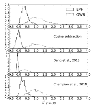
Figure 5: In the upper panel are shown the normalized $\hat{\rm A}^{2}$ distributions as computed for simulations S_eph (solid histograms) and S_gwb (dotted histogram). In the central and bottom panels we show the same distributions, after the application of the two mitigation routines described in this Section (4.3).

We therefore conclude that:

• Without correction, planetary ephemeris errors may yield sufficiently large $\hat{\rm A}^{2}$ values to lead to false detections when searching for a GWB in PTA data sets;

• Fitting a cosine to the angular covariances, as well as the Hellings & Downs curve, removes the bias resulting from random ephemeris errors but does not reduce the noise in the A² estimator: the standard deviation is not significantly reduced;

• Using the Deng et al. (2013) approach does correct the ephemeris errors, but also absorbs significant power from the GWB signal;

• If the error in the ephemeris was known to be solely caused by errors in planet masses then one can use the Champion et al. (2010) method, which does not significantly affect the GWB search.

In these sections we simulated red noise processes that have an identical power spectrum as a GWB with $A=10^{-15}$. Hereafter, we consider other noise processes that may be present in the data, but have different spectral shapes.

4.4 Realistic clock and ephemeris error levels

It is challenging to determine the actual amount of noise from the clock or ephemeris errors in real PTA data. We can consider the signals injected in S_tt and S_de to be upper estimates of the real noise processes given by clock and ephemeris errors. Nevertheless, we are aware that the real errors might actually be higher. This could be caused by, e.g., still unknown systematics in the analysis algorithms or, in the case of the ephemeris, the occurrence of unknown bodies in the solar system or the influence of asteroids. For instance Hilton & Hohenkerk (2011) compare three different ephemerides and note that the JPL ephemeris does not include a ring of asteroids that can shift the position of the barycentre by $\sim 100$ m. The results shown in Table 3 indicate that none of the $\hat{\rm A}^{2}$ distributions obtained for S_tt and S_de are consistent with zero.

In the top panel of Figure 6 we show the power spectra for S_tt and S_de, averaged over the 20 pulsars simulated for one realization, along with the theoretical power spectrum of a GWB with A = 10^-15. The power spectrum of S_tt is higher than the GWB’s, roughly corresponding to a background amplitude of 2.1$\times$10^-15. The approximate equivalent amplitude of S_de is lower, about 7.3$\times$10^-16. However, the slopes of the two spectra are very similar to the predictions for a GWB.

In Figure 7 we show DT5 obtained for the S_tt and S_de simulations without (solid bars) and with (dashed bars) mitigation methods being applied (the Hobbs et al. 2012 and the Champion et al. 2010 methods respectively). We also show the ranges of the GWB amplitude as predicted by four recent models (Gaussian functions shown at the bottom of the figure). The shaded region designates the 95% upper limit on A² (Shannon et al., submitted).

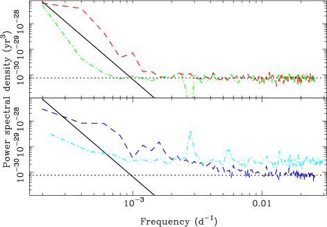
Figure 6: Power spectra averaged over the 20 simulated pulsars for S_tt (dashed line) and S_de (dot-dashed line) are shown in the top panel. S_ie at 200 ns (dashed line) and S_sw (dot-dashed line) are shown in the bottom panel. In both panels the expected power spectral density for a GWB with A = 10^-15 is shown as the black solid line. The power spectral density corresponding to 100 ns of white noise is indicated as the black dotted line.

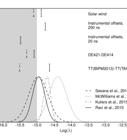
Figure 7: In the lower part of the diagram we show the GWB amplitude ranges expected by four recent GWB models (fourth model of Sesana 2013b, McWilliams et al. 2014, Kulier et al. 2015 and Ravi et al. 2015. The shaded region designates the latest 95% upper bound to A² (Shannon et al., submitted). In the upper part of the Figure, we show the 95% $\hat{\rm A}^{2}$ levels as obtained for S_tt, S_de, S_ie (at 20 and 200 ns) and S_sw. The solid and dashed (if present) bars indicate, respectively, the 95% bound without and with (dashed) mitigation algorithm (the Hobbs et al. 2012 for the clock errors, the Champion et al. (2010) for the ephemeris errors and the default tempo2 model for the solar wind effects.

For all the simulated effects different from a GWB, the range of the $\hat{\rm A}$ estimators show a non-negligible degree of overlap with the GWB amplitude interval predicted by some of the most recent models. In particular, this plot indicates that the clock errors of S_tt are likely to be the most significant source of false detections. However, as shown in Section 4.2, clock errors can be mitigated using one of the algorithms that we described. Errors in the ephemeris are at a smaller amplitude. They can also lead to significant false detections if the actual GWB amplitude is lower than $\sim 10^{-15}$ (as the current upper limit on the GWB amplitude indicates). All the mitigation methods that we have considered for planetary ephemeris errors have problems. For instance, the Champion et al. (2010) can only be applied to errors in the masses of known objects. Champion et al. (2010) suggested that the only likely sources of error are in the masses of Jupiter and/or Saturn. With recent spacecraft flybys these errors are likely to be small, and can easily be corrected using the Champion et al. (2010) procedure without affecting any underlying GWB. The method could, if necessary, also be updated to account for the poorly known mass of any asteroid that is expected to produce a significant residual. Previously unknown objects are more easy to deal with by using the Deng et al. (2013) method. However, that method currently absorbs a significant part of the GWB signal. We are therefore studying whether that method can be modified so that it does not significantly affect any GWB signal, by, for example, ensuring that all errors in the ephemeris are caused by orbiting bodies with a prograde or retrograde motion, or constraining the errors to be close to the ecliptic plane.

We outline below an illustrative procedure to confirm that a GWB detection is not caused by clock and ephemeris errors:

• It is always valid to remove a constant offset and a cosine function from the covariances before (or while) fitting the Hellings & Downs curve. This leads to a small reduction in the amplitude of the GWB, but that can be subsequently calibrated and it eliminates the possibility of a false alarm caused by clock or certain types of ephemeris errors.

• If the constant offset measurement is statistically significant then we recommend first measuring the clock errors (using e.g., the Hobbs et al., 2012 method), removing them and then searching again for the GWB accounting for the subtracted signal.

• If the cosine term is statistically significant then it is likely that an ephemeris error is present. Mitigating such errors will depend upon their nature. We can apply the Deng et al. (2013) procedure, reducing its impact on the GWB search by rotating the resulting vector components into the ecliptic plane. If the error is constrained to the ecliptic plane, it would be possible to fit only for two components of $\mathbf{e}$. The power spectra of these components may also indicate excess power at the period of a known planet. If so, one can apply the Champion et al. (2010) method. A final search could be carried out to determine whether the errors corresponded to prograde or retrograde orbits. If true, then a fit to such errors can be carried out, thereby further reducing the noise.

• If the GWB detection is still significant after the above procedure, then it will be necessary to determine the false alarm probability of the measured $\hat{\rm A}^{2}$ value and we note that, if the GWB amplitude is at the low end of the ranges ranges predicted by the models, then the signals we simulated can induce false detections even after being “mitigated”.

4.5 Other correlated errors

4.5.1 Instrumental errors

For S_ie, the pulsar data sets are correlated - all instrumental jumps occur at the same epoch. However, the measured covariances (Figure 2) depend upon the size of the offsets. An offset introduced by a receiver or processing system upgrade might be up to a few microseconds. Individual cases can be fitted and removed, but these removal procedures might leave residual offsets up to tens or hundreds of nanoseconds. The power spectral density for 200 ns offsets is shown in the bottom panel of Figure 6. The power spectral density for smaller offsets can be estimated by simply scaling the line shown in this Figure. For instance, offsets of 20 ns would have a power spectral density that is 100 times smaller than that shown for the 200 ns offsets.

As Table 3 shows, in the case of S_ie at 20 ns, the mean of the resulting $\hat{\rm A}^{2}$ distribution is statistically consistent with zero, and DT5 is zero: the distribution does not overlap with the results from S_gwb. However, with a residual error size of 200 ns, the standard deviation increases by a factor $\sim 30$. In this case, the $\hat{\rm A}^{2}$ values do overlap those from S_gwb. The shape of the angular correlations suggests that these signals are unlikely to be misidentified with a GWB. Nevertheless, such uncertainties do exist in real time series, and only careful inspection of the data can ensure that they do not interfere with the GWB detection.

4.5.2 Solar wind

The power spectral density of the residuals induced by the solar wind is shown as the dot-dashed line in Figure 6. This power spectral has a complex form. The entire white noise level is higher than given by the simulated white noise level (i.e., the solar wind is inducing excess white noise). A clear excess in power is observed with a 1 year periodicity and there is an increase in power at low frequencies.

The solar-wind simulations S_sw require more pre-processing than the others. When the line-of-sight to these pulsars passes close to the Sun, the effects of the solar wind can become extremely large (Table 1 shows that two of the pulsars, PSRs J1022+1001 and J1730$-$2304, have an ecliptic latitude of less than one degree). In these conditions, PTA teams usually do not collect ToAs.

We chose a conservative approach, by excluding simulated observations within 14 degrees from the Sun. As the routines used to simulate the effect of the solar wind (described in detail in You et al. 2007) have a degeneracy near to 180 degrees, we also excluded these observations.

Figure 2 shows that pulsar pairs with small and large angular distances are, respectively, correlated and anti-correlated. Table 3 shows that the $\hat{\rm A}^{2}$ distribution obtained for S_sw is narrower than the S_gwb by a factor $\sim 4$, but the mean is slightly higher: 1.6$\times 10^{-30}$.

An attempt to mitigate the impact of the solar wind is implemented in tempo2 and is applied by default. This process simply assumes a constant, spherically symmetric model for the solar wind and predicts the residuals based on the angle between the line-of-sight to the pulsar and the Sun. The electron density at 1 AU is set to 4 cm^-3 by default (an analogous model is available in the tempo software package, with an electron density of 10 cm^-3 at 1 AU). As shown in Table 3 the application of this method reduces the mean of the obtained $\hat{\rm A}^{2}$ distribution by a factor of $\sim$4.

Since the solar wind variability induces fluctuations in the DM values, it is also possible to attempt a mitigation by applying existing algorithms that model the DM variations. The method of Keith et al. (2013) is the one that is currently adopted by the PPTA for the same purpose, and uses multi-frequency data in order to obtain a grid of time-dependent DM values, computed as averaged estimates over the duration of the grid steps. Simultaneously, the frequency-independent noise over the same grid steps is modeled in order to avoid misidentifying frequency-independent timing noise as DM variations.

We do not simulate multi-frequency data. However, we can adapt the Keith et al. (2013) method by attributing every offset in the time series to DM variations caused by the solar wind. This is possible, as we know the simulated data that we are dealing with in this section do not contain any other low-frequency noise besides the solar wind signal. We thus estimated and removed the DM fluctuations by using a grid step of 100 days, independently for each pulsar. This method is not particularly effective. Although it strongly reduces the standard deviation of the A² distribution, it leaves the mean almost unaltered. The most likely explanation for this result is that the variations caused by the solar wind are narrow and cuspy. They are not well modeled by linear interpolation of DM variations on a 100 day timescale.

The other PTA teams typically use different methods to assess the effects of DM fluctuations. The EPTA relies on a Bayesian analysis of the red noise processes, and assumes a 2-parameter power law to model the spectrum of the DM variations (Lentati et al., 2013). Nanograv includes the effect of DM fluctuations in time offsets that remain constant over a 15-day window (Demorest et al., 2013).

The impact of the solar wind may be minimized by observing at the highest feasible frequency. However, as it is difficult to remove it completely, a simulation of the solar wind effects should be included to estimate the false alarm probability of any GWB detection. Further work on this topic would be extremely valuable.

4.6 The role of the IPTA

We have shown that correlated noise processes present in PTA data, if sufficiently large, will affect the GWB search. We have only made use of a single, frequentist-based detection method, but our results will also be applicable to any frequentist or Bayesian detection routine as all the PTA detection algorithms rely on the same basic principles (that of maximum likelihood). Moreover, even though we can develop mitigation routines to account for most of these noise processes, unexpected correlated signals will also exist in the data.

None of the non-GWB noise processes that we simulated led to angular covariances that were identical to the Hellings & Downs curve (Figure 2). This curve has positive correlations for small angular separations and for separations close to 180 degrees and negative correlations around 90 degrees. A robust detection of the GWB would therefore include strong evidence of this specific shape to the angular covariances. The PPTA pulsars offer a good sampling of the angular separations between $\sim$25 and $\sim$140 degrees (see Figure 1), but they poorly cover the closest and the widest angular separations. To make a robust detection of the GWB even more challenging, the PPTA pulsars are non-homogeneous. A few pulsars are observed with significantly better timing precision than other pulsars.

In contrast, the IPTA contains a much larger sample of pulsars (the current IPTA observes a sample of about 50 pulsars, although, as for the PPTA, the pulsars are non-homogeneous) covering a wider range of angular separations (shown in black dots in Figure 1). It will therefore be significantly easier to present a robust detection of the GWB with IPTA data than with PPTA data alone. The IPTA also provides other ways to reduce the chance of false detections. For instance, multiple telescopes observe the same pulsars: a comparison between data sets from different telescopes will allow us to identify instrumental and calibration errors, along with other issues such as errors in the time transfer from the local observatory clocks. The increased number of observing frequency bands will also enable the IPTA data to be corrected for dispersion measure and possibly solar wind effects more precisely than they could by a single timing array project.

5 Summary and Conclusions

We have simulated various correlated noise processes that might affect PTA pulsar data. We studied their effect on the GWB search by using a PPTA detection code based on a frequentist approach. We also tested mitigation routines for some of the simulated signals. Our main conclusions are that:

• blind use of a detection code without mitigation routines can lead to false identifications of a GWB signal;

• errors in the terrestrial time standard are expected to have the largest effect, but such errors can be mitigated without affecting any underlying GWB signal;

• errors in the planetary ephemeris will become important if the GWB signal is significantly lower than the current upper bounds. It is not trivial to develop an effective mitigation routine that does not affect the underlying GWB signal;

• the effect of instrumental errors scales with their amplitude. Small offsets are unlikely to cause false detections. Much larger offsets may do so;

• the solar wind will yield false detections if not properly modeled;

• other correlated signals may be present in a PTA data set and may affect a GWB search.

With care, a robust detection of the GWB can be made. However, determining all the physical phenomena that can affect the data is challenging and the combined data sets of the IPTA will be necessary to provide confident detections of the GWB.

Appendix A Signature of an error in the planetary ephemeris

Errors in the terrestrial time standard lead to the same induced timing residuals for different pulsars. The covariance between different pulsar pairs can therefore easily be determined. However, determining the covariances between pulsar pairs caused by an error in the planetary ephemeris is more challenging and we derive the expected covariance here.

The timing residuals of a planetary ephemeris error are given by Equation 3. The covariance $C(\theta_{ij})$ between the residuals for two pulsars $i$ and $j$ induced by such an error is:

$$C(\theta_{ij})=\frac{1}{c^{2}}\langle({\bf e}\cdotp{\bf\hat{k}}_{\rm i})({\bf e}\cdotp{\bf\hat{k}}_{\rm j})\rangle$$ (10)

where, as in Equation 3, $\bf e$ is the time-dependent error in position of the SSB with respect to the observatory, $\bf\hat{k}_{\rm i}$ and $\bf\hat{k}_{\rm j}$ are unit vectors pointed toward pulsars $i$ and $j$. The ensemble averages are determined over each observation. We write:

$${\bf e}\cdotp{\bf\hat{k}}_{\rm i} = |{\bf e}|\cos{\alpha_{i}}$$ (11)

$${\bf e}\cdotp{\bf\hat{k}}_{\rm j} = |{\bf e}|\cos{\alpha_{j}}$$ (12)

and note that $\theta_{ij}$ has already been defined as the angle between the two pulsars.

Applying the cosine formula for a spherical triangle we have:

$$C(\theta_{ij})=(1/c^{2})\left(\langle|{\bf e}|^{2}\cos{\theta_{ij}}\rangle-\langle|{\bf e}|^{2}\sin\alpha_{i}\sin\alpha_{j}\cos{\beta}\rangle\right)$$ (13)

where $\beta$ is the angle subtended at e by $\hat{k}_{\rm i}$ and $\hat{k}_{\rm i}$ in the spherical triangle connecting the ends of the unit vectors.

If the error vector $\bf e$ is uncorrelated with the pulsar directions, the second term goes to zero and thus:

$$C(\theta_{ij})=\langle|{\bf e}|^{2}\rangle\cos{\theta_{ij}}/c^{2}.$$ (14)

In this case, the expected covariances will therefore have a cosinusoidal shape. Of course, a mass error in a specific planet leads to a deterministic error. However, errors induced by a large number of small masses may have a more different form. We therefore note that the actual covariances measured will only show a clear cosinusoidal form if this term dominates the second term in Equation 13.

References

- Champion et al. (2010) Champion D. J. et al., 2010, apjl, 720, L201
- Coles et al. (2011) Coles W., Hobbs G., Champion D. J., Manchester R. N., Verbiest J. P. W., 2011, MNRAS, 418, 561
- Demorest et al. (2013) Demorest P. B. et al., 2013, ApJ, 762, 94
- Deng et al. (2013) Deng X. P. et al., 2013, Advances in Space Research, 52, 1602
- Edwards et al. (2006) Edwards R. T., Hobbs G. B., Manchester R. N., 2006, MNRAS, 372, 1549
- Hellings & Downs (1983) Hellings R. W., Downs G. S., 1983, ApJ, 265, L39
- Hilton & Hohenkerk (2011) Hilton J. L., Hohenkerk C. Y., 2011, in Journées Systèmes de Référence Spatio-temporels 2010, Capitaine N., ed., pp. 77–80
- Hobbs et al. (2010) Hobbs G. et al., 2010, Classical and Quantum Gravity, 27, 084013
- Hobbs et al. (2012) Hobbs G. et al., 2012, MNRAS, 427, 2780
- Hobbs et al. (2009) Hobbs G. et al., 2009, MNRAS, 394, 1945
- Keith et al. (2013) Keith M. J. et al., 2013, MNRAS, 429, 2161
- Kramer & Champion (2013) Kramer M., Champion D. J., 2013, Classical and Quantum Gravity, 30, 224009
- Kramer et al. (2006) Kramer M. et al., 2006, Science, 314, 97
- Kulier et al. (2015) Kulier A., Ostriker J. P., Natarajan P., Lackner C. N., Cen R., 2015, ApJ, 799, 178
- Lee et al. (2014) Lee K. J. et al., 2014, MNRAS, 441, 2831
- Lentati et al. (2013) Lentati L., Alexander P., Hobson M. P., Taylor S., Gair J., Balan S. T., van Haasteren R., 2013, prd, 87, 104021
- Lentati et al. (2015) Lentati L. et al., 2015, ArXiv e-prints
- Lorimer et al. (2006) Lorimer D. R. et al., 2006, MNRAS, 372, 777
- Manchester et al. (2013) Manchester R. N. et al., 2013, PASA, 30, 17
- Manchester & IPTA (2013) Manchester R. N., IPTA, 2013, Classical and Quantum Gravity, 30, 224010
- McLaughlin (2013) McLaughlin M. A., 2013, Classical and Quantum Gravity, 30, 224008
- McWilliams et al. (2014) McWilliams S. T., Ostriker J. P., Pretorius F., 2014, ApJ, 789, 156
- Phinney (2001) Phinney E. S., 2001, e-prints (arXiv:astro-ph/0108028)
- Ravi et al. (2012) Ravi V., Wyithe J. S. B., Hobbs G., Shannon R. M., Manchester R. N., Yardley D. R. B., Keith M. J., 2012, apj, 761, 84
- Ravi et al. (2015) Ravi V., Wyithe J. S. B., Shannon R. M., Hobbs G., 2015, mnras, 447, 2772
- Sesana (2013a) Sesana A., 2013a, Classical and Quantum Gravity, 30, 244009
- Sesana (2013b) Sesana A., 2013b, Classical and Quantum Gravity, 30, 224014
- Sesana et al. (2009) Sesana A., Vecchio A., Volonteri M., 2009, MNRAS, 394, 2255
- Shannon & Cordes (2010) Shannon R. M., Cordes J. M., 2010, apj, 725, 1607
- van Haasteren et al. (2011) van Haasteren R. et al., 2011, MNRAS, 414, 3117
- Wang et al. (2012) Wang J., Wang N., Tong H., Yuan J., 2012, Astrophysics and Space Science, 340, 307
- Yardley et al. (2011) Yardley D. R. B. et al., 2011, MNRAS, 414, 1777
- You et al. (2012) You X. P., Coles W. A., Hobbs G. B., Manchester R. N., 2012, mnras, 422, 1160
- You et al. (2007) You X. P., Hobbs G. B., Coles W. A., Manchester R. N., Han J. L., 2007, ApJ, 671, 907