Quantum transport through a molecular level: a scattering states numerical renormalisation group study

Abstract

We use the scattering states numerical renormalization group (SNRG) approach to calculate the current $I(V)$ through a single molecular level coupled to a local molecular phonon. The suppression of $I$ for asymmetric junctions with increasing electron-phonon coupling, the hallmark of the Franck-Condon blockade, is discussed. We compare the SNRG currents with recently published data obtained by an iterative summation of path integrals approach (ISPI). Our results excellently agree with the ISPI currents for small and intermediate voltages. In the linear response regime $I(V)$ approaches the current calculated from the equilibrium spectral function. We also present the temperature and voltage evolution of the non-equilibrium spectral functions for a particle-hole asymmetric junction with symmetric coupling to the lead.

I Introduction

In the quest for size-reduced and possible low-power consuming electronic devices, the proposal Aviram and Ratner (1974) of using molecular junctions for electronics has sparked a large interest in understanding the influence of molecular vibrational modes onto the electron charge transfer through a molecule. The non-linear current through a molecule device can be controlled by a capacitively coupled external gate Chen et al. (1999); Donhauser et al. (2001). Interestingly, hysteretic behavior of the $I(V)$ curves Li et al. (2003) has been reported in several experiments when sweeping the voltage with a finite rate. However, the observed hysteresis are non-universal and depend on the sweeping rate. For infinitesimally slow sweeping the effect vanishes. In some cases a sudden drop of the current has been observed with increasing bias voltage Chen et al. (1999) which translates into a negative differential conductance. This all has been accounted to configural changes of the molecule emphasizing the importance of vibrational couplings in such devices.

Many experimental facts have been gathered in the last two decades but there is still a lack of an accurate theoretical description of all the reported phenomena. An excellent review Galperin et al. (2007) by Galperin et al. comprehensively summarizes the different theoretical approaches and experimental findings. Single molecular transistors (SMT) promise to offer some advantages over their semi-conductor based counterparts Kastner (1992). Both types of single-electron transistors can be controlled by a capacitively coupled external gate Kastner (1992); Chen et al. (1999); Donhauser et al. (2001). The molecular energy scales, however, are larger in SMTs and reproducibly defined by the chemistry of the molecule. In addition, the coupling to vibrational modes enlarges the parameter space and different physics such a phonon-assisted tunneling, Frank-Condon blockade or the appearance of inelastic steps in the $I(V)$ curve can be observed.

The theoretical description of such molecular junctions only include those molecular levels and vibrationals modes relevant for the quantum transport. The simplest model proposed Galperin et al. (2005, 2004, 2007) comprise a single level coupled to a local Holstein phonon. Typically rate equations Koch and von Oppen (2005) or lowest order Keldysh-Green function approaches Galperin et al. (2007); Koch et al. (2011, 2012) have been applied to this problem Galperin et al. (2005). Recently, the iterative path-integral approach (ISPI) Weiss et al. (2008) has also been successfully applied Hützen et al. (2012) to calculate quantum transport for moderate and high temperatures compared to the charge-transfer rate $\Gamma_{0}$.

The equilibrium physics of two extreme limits have been well understood in a model containing only a single vibrational mode Galperin et al. (2007); Koch and von Oppen (2005); Eidelstein et al. (2013). In the adiabatic limit, the phonon frequency is the smallest energy scale of the problem and a small electron-phonon coupling yields a reduction of the phonon frequency by particle-hole excitations. This limit has been pioneered by Caroli et al.Caroli et al. (1971); *Caroli72 in the context of tunnel junctions and applied to molecular junctions Galperin et al. (2004) .

In the opposite limit, for very small tunneling rates $t_{\alpha}$ one starts from the exact solution of the local problem by applying a Lang-Firsov transformation Lang and Firsov (1962). A displaced phonon with an unrenormalized phonon frequency $\omega_{0}$ and a polaron with a shifted single-particle energy is formed locally. In this anti-adiabatic limit, the strong electron-phonon coupling yields a polaronic shift of the single-particle level and a exponential suppression of tunneling rate related to the Franck-Condon blockade Koch and von Oppen (2005); Galperin et al. (2007); Leturcq et al. (2009); Hützen et al. (2012).

Wilson’s numerical renormalization group (NRG) approach Wilson (1975); Bulla et al. (2008) has been adapted to the Holstein model in equilibrium Hewson and Meyer (2002). A comprehensive study Eidelstein et al. (2013) has demonstrated the power of this non-perturbative approach to reveal the interplay between the different energy scales of the problem in the crossover regime. In this article we review the extension Jovchev and Anders (2013) of the approach to steady-state currents by applying the scattering-states NRG (SNRG) Anders (2008a); Schmitt and Anders (2010, 2011) to the spinless Anderson-Holstein model.

II Theory of Quantum transport through molecular junction

II.1 Model

In molecular electronics experiments Chen et al. (1999); Donhauser et al. (2001), a complex organic molecule is contacted by two conducting leads. We have modeled these leads as two symmetric featureless free electron gases since the mean-free path in the leads is large compared to the spatial dimensions of the device. In general, the molecule can contain several molecular orbitals which are actively participating in the quantum transport. Furthermore, the internal vibrational modes of the molecule are influenced by charging and discharging of the molecule.

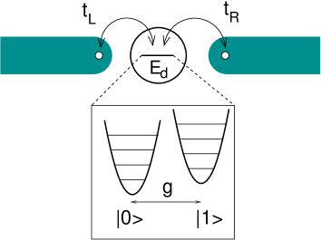
Figure 1: Minimal model of a molecule consisting of a single active molecular level at energy $E_{d}$ coupled to two leads with tunneling matrix elements $t_{L}$ and $t_{R}$. Depending on the local charge configuration $|0\rangle$ or $|1\rangle$, the ground state of a vibrational degree of freedom is shifted. The relative displacement between the two configuration is given by the dimensionless electron phonon coupling $g=\lambda_{ph}/\omega_{0}$. The phononic excitations for a fixed charge are multiples of the oscillator energy $\omega_{0}$.

Here we consider the most minimalistic model for quantum transport through a molecule Koch and von Oppen (2005); Galperin et al. (2007); Hützen et al. (2012) and follow the notation of Ref. Jovchev and Anders (2013). This widely used Hamiltonian Galperin et al. (2007); Hützen et al. (2012); Eidelstein et al. (2013) is defined as

$$H = E_{d}d^{\dagger}d+\omega_{0}b^{\dagger}b+\lambda_{ph}(b^{\dagger}+b)\left(\hat{n}_{d}-\frac{1}{2}\right)$$ (1)

$$+\sum_{\alpha=L,R}\sum_{k}\varepsilon_{k\alpha}c^{\dagger}_{k\alpha}c_{k\alpha}$$

$$+\sum_{\alpha=L,R}\frac{t_{\alpha}}{\sqrt{N}}\sum_{k}(d^{\dagger}c_{k\alpha}+c^{\dagger}_{k\alpha}d)$$

where $d(d^{\dagger})$ annihilates(creates) an electron on the device with energy $E_{d}$, and $c^{\dagger}_{k\alpha}$ creates an electron in the lead $\alpha$ with energy $\varepsilon_{k\alpha}$. The local charge-transfer rate to each lead $\alpha$ is given by $\Gamma_{\alpha}=\pi t_{\alpha}^{2}\rho_{\alpha}(0)$, where $\rho_{\alpha}(\omega)$ is the density of states of lead $\alpha$. In order to focus only on the influence of the electron-phonon interaction onto the quantum transport, the spin degree of freedom is neglected in order to avoid obstruction of the competition between spin-flip scattering through the device and polaron formation on the device.

The model comprise a single active molecular level - all others are energetically well separated – whose charge density is coupled to a local Holstein phonon stemming from the dominating vibrational mode of the molecule. In real materials, band features are important but only influence the single-particle properties which can be accounted for in a frequency dependent charge transfer rate $\Gamma_{\alpha}(\omega)$ which we treat as a constant for simplicity in our simulations.

The spinless Anderson-Holstein model is schematically depicted in Fig. 1. Depending on the local charge configuration, the local harmonic oscillator is displaced and the dimensionless distance between the two ground states is given by $g=\lambda_{ph}/\omega_{0}$. For modeling realistic situations, the restriction to a single phonon and a single electronic level must be lifted. In spite of a lot of theoretical progress Galperin et al. (2007) this model has only been accurately solved in equilibrium Hewson and Meyer (2002); Vinkler et al. (2012); Eidelstein et al. (2013), while its non-equilibrium dynamics has only be perturbatively investigated in lowest order of the coupling constants Galperin et al. (2007).

The local Hamiltonian is given by the first line in (1) and can be solved exactly using the Lang-Firsov transformation Lang and Firsov (1962); Mahan (1981). This local solution consists of a local polaron decoupled from a shifted harmonic oscillator. The corresponding polaronic energy gain is given by $E_{p}=\lambda_{ph}^{2}/\omega_{0}=g^{2}\omega_{0}$.

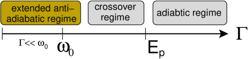
Figure 2: The different regimes as function of the charge transfer rate $\Gamma_{0}$. The crossover from extended anti-adiabatic regime is reached when $\Gamma_{\rm eff}\approx e^{-g^{2}}\Gamma_{0}\approx\omega_{0}$ and extents to $\Gamma\approx E_{p}=g^{2}\omega_{0}$.

Coupling this local degrees of freedom to the two leads defines two competing regimes depicted in Fig. 2. For $E_{p},\omega_{0}\ll\Gamma_{0}=\Gamma_{L}+\Gamma_{R}$, the phonon dynamics is slow and can be treated perturbatively in this adiabatic regime. $E_{p},\omega_{0}\gg\Gamma_{0}$ defines the opposite limit: in this anti-adiabatic regime charge fluctuations are suppressed, the electron moves slow and the phonon defines the large energy scale. The anti-adiabatic regime is relevant for molecular junctions since the tunneling coupling of a molecule to the leads is usually small compared to the intrinsic energy scales of the molecule. After the Lang-Firsov transformation, the tunneling term acquires an additional factor $\exp[g(b^{\dagger}-b)]$ whose physical meaning is stripping the original electron content from the locally formed polaron. If $\omega_{0}\gg\Gamma$, the local phonon remains in its ground states which yields an exponential suppression of the tunneling coupling and $\Gamma\to\Gamma_{\rm eff}\approx\Gamma_{0}e^{-g^{2}}$. In a particle-hole asymmetric junction, this leads to a Franck-Condon suppression of the current for small bias voltage: The system reacts with a dynamical suppression of the tunneling rate to avoid the reorganization of the nuclear positions of the molecule.

II.2 Scattering-states numerical renormalization group

The scattering-states numerical renormalization group (SNRG) approach is based on the steady-state density operator $\rho(\mu_{L},\mu_{R})$ for a current carrying ensemble Hershfield (1993) coupled to two baths at different chemical potentials $\mu_{\alpha}$. Hershfield has shown Hershfield (1993) that this operator has a Boltzmannian form

$$\hat{\rho}(\mu_{L},\mu_{R}) = \frac{1}{Z}e^{-\beta(H-Y)}$$ (2)

where $Z$ is the partition function and $\mu\hat{N}$ is replaced by the $Y$-operator. This $Y$-operator is in general unknown for a arbitrary fully interacting Hamiltonian.

For a non-interacting problem, however, the corresponding $Y_{0}$-operator is given in terms of the Lippmann-Schwinger scattering states with energy $\varepsilon$ of left-moving or right moving single-particle scatting state created by $\gamma^{\dagger}_{\alpha}(\varepsilon)$,

$$Y_{0} = \sum_{\alpha}\mu_{\alpha}\int d\varepsilon\,\gamma^{\dagger}_{\varepsilon\alpha}\gamma_{\varepsilon\alpha}$$ (3)

where $\{\gamma^{\dagger}_{\varepsilon\alpha},\gamma^{\dagger}_{\varepsilon^{\prime}\alpha^{\prime}}\}=\delta_{\alpha\alpha^{\prime}}\delta(\varepsilon-\varepsilon^{\prime})$. Note that the applied source-drain voltage $eV=\mu_{L}-\mu_{R}$.

In the SNRG Anders (2008a); Schmitt and Anders (2010) we have circumvented the unknown $Y$ by the following procedure.

First, we realise that we can discretize the energy dependent scattering states on a logarithmic energy mesh identically as in the standard NRGBulla et al. (2008); Anders (2008a) such that we obtain a two-band model comprising of a left-mover and right-mover band. (Below, we will comment on the analytical form of the scattering states.) Then we perform a standard NRG using $K_{0}=H(\lambda_{ph}=0)-\hat{Y}_{0}$.

Knowing the analytical form of the non-equilibrium density operator $\hat{\rho}_{0}(V)=\exp(-\beta K_{0})/Z_{0}$, we can discretize scattering states on a logarithmic energy mesh identically to the standard NRG Bulla et al. (2008); Anders (2008a) and perform an NRG using $K_{0}=H(\lambda_{ph}=0)-\hat{Y}_{0}$. The density operator $\hat{\rho}_{0}(V)$ contains all information about the current carrying steady-state for the Hamiltonian $H_{0}=H(\lambda_{ph}=0)$ Hershfield (1993).

Starting at time $t=0$, we let the non-interacting system propagate with respect to the full Hamiltonian $H_{f}=H(\lambda_{ph}>0)$: The density operator $\hat{\rho}(t)$ progresses as $\hat{\rho}(t)=\exp(-iH_{f}t)\rho_{0}\exp(iH_{f}t)$. Since we quench the system only locally, we can assume $\hat{\rho}(t)$ reaches a steady-state at $t\to\infty$ independent of initial condition for an infinitely large system: all bath correlation functions decay for infinitely long times. The finite size oscillations always present in the NRG calculation Anders and Schiller (2005, 2006); Anders (2008a); Eidelstein et al. (2012); Guettge et al. (2013) are projected out by defining the time-averaged density operator Suzuki (1971); Anders (2008a)

$$\hat{\rho}_{\infty} = \lim_{T\to\infty}\frac{1}{T}\int_{0}^{T}dt\hat{\rho}(t)\,.$$ (4)

Consequently, only density matrix elements diagonal in energy contribute to the steady-state in accordance with the condition $[H_{f},\hat{\rho}_{\infty}]=0$. Even though the $Y$-operator remains unknown, we explicitly construct a numerical representation of the non-equilibirum density matrix using the time-dependent NRG Anders and Schiller (2005); *AndersSchiller2006; Eidelstein et al. (2012). In a last step, we calculate local steady-state retarded Green function

$$G^{r}_{d,d^{\dagger}}(t) = -i\textrm{Tr}\left[\hat{\rho}_{\infty}\{d(t),d^{\dagger}\}\right]\Theta(t),$$ (5)

where $d(t)=e^{iH_{f}t}de^{-iH_{f}t}$ and $\hat{\rho}_{\infty}$ has been defined in Eq. (4). The approach is based on an extension for equilibrium Green functions Peters et al. (2006) and its technical details are found in Ref. Anders, 2008b.

It has been show Meir and Wingreen (1992); Hershfield (1993); Oguri (2007) that for the model investigated here, the current is given by the by a generalized Landauer formula

$$I(V) = \frac{G_{0}}{e}\int_{-\infty}^{\infty}\,d\omega\,\left[f_{R}(\omega)-f_{L}(\omega)\right]\Gamma_{0}\pi\rho_{d}(\omega,V)$$ (6)

where $f_{\alpha}(\omega)=f(\omega-\mu_{\alpha})$ and the steady-state spectral function $\pi\rho_{d}(\omega,V)=\Im m[G^{r}_{d,d^{\dagger}}(\omega-i0^{+},V)]/\pi$ is obtain from the Fourier transformed retarded Green function Eq. (5). The prefactor

$$G_{0} = \frac{e^{2}}{h}\frac{4\Gamma_{L}\Gamma_{R}}{\Gamma_{0}^{2}}$$ (7)

contains the leading asymmetry factors of the junction and reaches the universal conductance quantum $e^{2}/h$ for a symmetric junction, i. e. $\Gamma_{L}=\Gamma_{R}$. $G_{0}$ can be expressed as $G_{0}=(e^{2}/h)(4R/(1+R)^{2})$ using the definition of the coupling asymmetry ratio $R=\Gamma_{L}/\Gamma_{R}$.

II.3 Single-particle scattering states

In the absence of the electron-phonon coupling, the Hamiltonian (1) can be solved exactly in terms of single-particle Lippmann-Schwinger scattering states Hershfield (1993); Schiller and Hershfield (1995); Oguri (2007); Anders (2008a),

$$H_{0} = \sum_{\alpha}\int d\varepsilon\,\varepsilon\,\gamma_{\varepsilon\alpha}^{\dagger}\gamma_{\varepsilon\alpha}$$ (8)

where

$$\gamma^{\dagger}_{\alpha} = c^{\dagger}_{\varepsilon\alpha}+t_{\alpha}\sqrt{\rho_{\alpha}(\varepsilon)}G_{0\sigma}^{r}(\varepsilon+i\delta)$$ (9)

$$\times\left[d^{\dagger}+\sum_{\alpha^{\prime}}\int d\varepsilon^{\prime}\frac{V_{\alpha^{\prime}}\sqrt{\rho_{\alpha^{\prime}(\varepsilon^{\prime})}}}{\varepsilon+i\delta-\varepsilon^{\prime}}c^{\dagger}_{\varepsilon^{\prime}\alpha^{\prime}}\right]$$

and the local resonant level Green function

$$G_{0}^{r}(z) = \left[z-E_{d}-\Delta(z)\right]^{-1}$$ (10)

$$\Delta(\omega-i\delta) = \sum_{\alpha}t^{2}_{\alpha}\int d\varepsilon\frac{\rho_{\alpha}(\varepsilon)}{\omega-\varepsilon}$$ (11)

enters as one of the expansion coefficients. $\rho_{\alpha}(\varepsilon)$ denotes the density of states of the individual leads and will be takes as equal and featureless in the following. The small imaginary part $i\delta$ is required for regularization in the transition from the discrete $k$ summation in Eq. (1) to the continuum limit an caused the time-reversal symmetry breaking.

Note that the $d$-orbital has been included into the scattering states. By inverting the unitary transformation, we can expand the local $d$-orbital in left-moving and right-moving scattering states.

$$d^{\dagger} = r_{R}d^{\dagger}_{R}+r_{L}d^{\dagger}_{L}$$ (12)

$$d^{\dagger}_{\alpha} = \bar{t}\int d\varepsilon\sqrt{\rho(\varepsilon)}[G_{0}^{r}(\varepsilon+i\delta)]^{*}\gamma^{\dagger}_{\varepsilon\alpha}$$ (13)

where we defined $\bar{t}=\sqrt{t_{L}^{2}+t_{R}^{2}}$ and have used $r_{\alpha}=t_{\alpha}/\bar{t}$. The expansion coefficients in Eq. (13) contain the retarded Green function $G_{0}^{r}(\varepsilon+i\delta)$ which we separate in modulus and phase

$$[G_{0}^{r}(\varepsilon+i\delta)] = |G_{0}^{r}(\varepsilon+i\delta)|e^{-i\Phi(\varepsilon)}.$$ (14)

This phase is absorbed into the new scattering states $\gamma^{\dagger}_{\varepsilon\alpha}\to\tilde{\gamma}^{\dagger}_{\varepsilon\alpha}=\gamma^{\dagger}_{\varepsilon\alpha}e^{i\Phi(\varepsilon)}$ by a local gauge transformation. In the wide band limit, i.e. $D\gg\Gamma_{0}$, the effective DOS $\tilde{\rho}(\varepsilon)=[\bar{t}\sqrt{\rho(\varepsilon)}|G_{0}^{r}(\varepsilon-i\delta)|]^{2}$ is normalized,

$$\int d\varepsilon\tilde{\rho}(\varepsilon) = \int d\varepsilon\left[\bar{V}\sqrt{\rho(\varepsilon)}|G_{0}^{r}(\varepsilon-i\delta)|\right]^{2}=1\,,$$ (15)

and $d^{\dagger}_{\alpha}$ is used as a starting vector for the Householder transformation Wilson (1975); Bulla et al. (2008) for constructing the discretized Wilson chain. Although the physical contained of the Wilson chain sites are different to the standard NRG Wilson (1975); Bulla et al. (2008) the analytical from is preserved Anders (2008a). Since the local gauge transformation has to applied to the local current operator, the current flow is related to $\sin(\Phi(\varepsilon))$ of the energy dependent scattering phase.

III Results

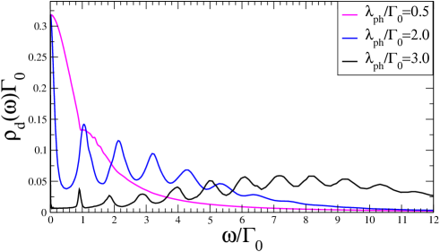
Figure 3: Equilibrium spectral function of the particle-hole symmetric junction, i. e. $E_{d}=0$, and $\omega_{0}/\Gamma_{0}=1$ for three different electron-phonon coupling strength $\lambda_{ph}/\Gamma_{0}=0.5,2,3$.

III.1 Equilibrium spectral function

To set the stage for the non-equilibrum steady state currents, we show the evolution of the equilibrium spectra function $\rho_{d}(\omega)$ for three different ratios $\lambda_{ph}/\Gamma$ in Fig. 3. While $\lambda_{ph}/\Gamma=0.5$ lies in the adiabatic regime, the two others are represents the anti-adiabatic regime. For $\lambda_{ph}/\Gamma=0.5$, we find a kink in the spectral function at $\omega_{0}$ where strong electron-phonon scattering sets in. For $\lambda_{ph}/\Gamma=2$ we observe already very pronounced phonon-replicas with a reduced width. Increasing $\lambda_{ph}/\Gamma$ further yields to a substantial shift of spectral weight from the resonance at $\omega=0$ to larger frequencies: a careful analysis shows Eidelstein et al. (2013); Jovchev and Anders (2013) that the peak of the envelope function is related to the effective Coulomb repulsion between the $d$-electron and the conduction band electrons which can be derived analytically for $t_{\alpha}\to 0$ using a Schrieffer-Wulff transformation Eidelstein et al. (2013).

III.2 Steady-state currents

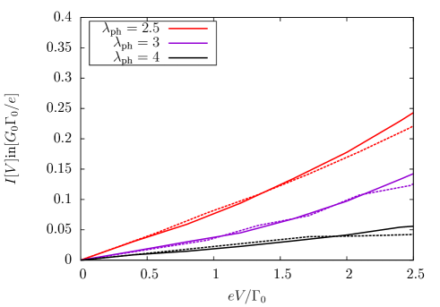
Figure 4: The evolution of $I(V)$ curves from medium to strong electron-phonon coupling for $T/\Gamma_{0}=0.2$ for a fixed phonon frequency $\omega_{0}/\Gamma_{0}=2$, a symmetric junction $\Gamma_{L}=\Gamma_{R}$ and level position in $H_{m}$, i. e. $\varepsilon=E_{d}+\lambda_{ph}^{2}/\omega_{0}=0$. A comparison between the SNRG data (straight lines) and the ISPI data (dotted lines), taken with permission from Ref. Hützen et al. (2012), is shown.

Recently, a numerical approach based on the iterative summation of path integrals (ISPI) Weiss et al. (2008) has been applied Hützen et al. (2012) to the model defined in Eq. (1). Since it requires a fast decay of the memory kernel for the discetized iterative summation of the path integral, it is restricted to moderate and high temperatures for large electron-phonon couplings. In this section, we will provide a comparison of the ISPI with the SNRG using the published ISPI data of Ref. Hützen et al. (2012).

It is straight forward to show that local Hamiltonian

$$H_{m} = \varepsilon d^{\dagger}d+\omega_{0}b^{\dagger}b+\lambda_{ph}(b^{\dagger}+b)\hat{n}_{d}$$ (16)

commonly used in the literature Galperin et al. (2005); Hützen et al. (2012) yield the same dynamics as the first three terms in Eq. (1) after identifying $\varepsilon=E_{d}+g^{2}\omega_{0}$ and performing a linear shift of the bosonic operators Eidelstein et al. (2013); Jovchev and Anders (2013).

Figure 4 shows the evolution of the current for a symmetric junction $\Gamma_{L}/\Gamma_{R}=1$ from medium to strong coupling at $T/\Gamma_{0}=0.2$, $\varepsilon=0$ and $\omega_{0}/\Gamma_{0}=2$. The overall agreement between the SNRG data (solid lines) and the ISPI approach (dotted lines) is remarkable up to $eV\approx 2\Gamma_{0}$ after which the small deviations become more pronounced: The SNRG current slightly exceeds the ISPI data for large voltages. Since both approaches, the ISPI and the SNRG, relay on discretisation of a continuum, we believe that the origin of these deviations are related to the different discretisation errors inherent in both methods.

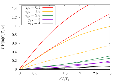
Figure 5: The evolution of $I(V)$ curves from weak to strong electron-phonon coupling for $T/\Gamma_{0}=1$ (dashed lines) and $T/\Gamma_{0}=0.2$ (straight lines) calculated with the SNRG. We have set $\omega_{0}/\Gamma_{0}=2$, a symmetric junction $\Gamma_{L}=\Gamma_{R}$ and $\varepsilon=E_{d}+\lambda_{ph}^{2}/\omega_{0}=0$.

The temperature dependency of the SNRG $I(V)$ curves are shown in Fig. 5 for two different temperatures. We combine the data of Fig. 4 for $T/\Gamma_{0}=0.2$ (straight lines) with the $I(V)$ for the same parameters but calculated at $T/\Gamma_{0}=1$ (dashed lines). In the limit $T\rightarrow\infty$ the currents must vanish: In this high temperature limit all left and right moving scattering states are equally occupied leading to zero net current as predicted by Eq. (6). For the electron-phonon couplings $\lambda_{\text{ph}}/\Gamma_{0}=0.5,1.5,2.5$, we clearly observe a decrease of the current with increasing temperature.

Above $\lambda_{\text{ph}}/\Gamma_{0}=3$, we observe a qualitative change of the behavior: the low temperature current is smaller than its high temperature counterpart: an indication of the Franck-Condon blockade in the quantum transport. There are two contributions changing the current according to Eq. (6) for a fixed voltage when raising the temperature. Firstly, the Fermi window becomes flatter and broader, and the high energy parts of the spectral function contribute stronger. In addition, the spectral function shows a significant temperature and voltage dependency with increasing electron-phonon coupling.

To illustrate this points, a comparison of nonequilibrium spectral functions with $\lambda_{\text{ph}}=3$ is depicted in Fig. 6 for two different temperatures and two different bias voltages. For $eV=0.8\Gamma_{0}$ an increase of temperature leads to a suppression of the phonon side peak at $\omega/\Gamma_{0}=-3$.

At the same time the peak at $\omega/\Gamma_{0}=-5$ is broadened and contributes more weight to the integral due to the broadened Fermi window, leading to an increase of the current with increasing temperature. At a voltage of $eV=3.2\Gamma_{0}$ the decrease of the spectral weight at $\omega/\Gamma_{0}=-3$ is not compensated within the Fermi window contributing to the current integral leading to a decrease of the current with increasing temperatures. Therefore, we observe a crossover between an increase of current at small voltages to an decrease of current at large voltages with increasing temperatures.

In contrary, the difference between the I-V curves of $T/\Gamma_{0}=1$ and $T/\Gamma_{0}=0.2$ are large at low phonon-couplings $\lambda_{\text{ph}}/\Gamma_{0}=0.5,1.5$. In this perturbative regime, the spectral function is only very weakly temperature dependent, and, therefore, the change of currents is only related to the temperature dependence of the Fermi functions in Eq. (6).

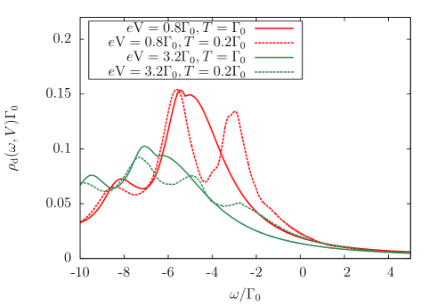
Figure 6: SNRG nonequilibrium spectral functions for two different voltages and two temperatures. We have set $\omega_{0}/\Gamma_{0}=2,\lambda_{ph}/\Gamma_{0}=3$ and $\varepsilon=E_{d}+\lambda_{ph}^{2}/\omega_{0}=0$.

III.3 Linear response regime

In order to explicit reveal the influence of the voltage dependency of the spectral function on the current $I(V)$, we compare the SNRG curves with the current calculated with the equilibrium spectral function $\rho_{d}(\omega,V)=\rho_{d}(\omega)$ in Eq. (6) neglecting its voltage dependency. The latter becomes asymptotically exact for $V\to 0$, defining the linear response regime. Deviations from these curves are caused by the voltage dependency of the true non-equilibrium spectral function. The results are depicted in Fig. 7 using the SNRG data of Fig. 5 for $T=\Gamma_{0}$. The SNRG curves (straight line) coincide with the equilibrium calculation (dashed line) in the linear response regime, i. e. $|eV|\ll\Gamma_{0}$. However, the larger the electron-phonon coupling, the smaller the validity range of the linear response regime. Already at very small finite voltages, we observe deviations from the I(V) generated by the equilibrium $\rho_{d}(\omega)$. The excellent agreement between the ISPI and the SNRG for $\lambda_{ph}/\Gamma_{0}=4$ results in the small voltage regime – see Fig. 4 – clearly demonstrates that the SNRG correctly accounts for the bias dependence of the spectral function.

IV Conclusion

We have applied the scattering states numerical renormalization group approach to the charge-transport through a symmetric molecular junction. Since we have focused on the influence of a vibronic mode on the transport, we have restricted ourselves to the investigation of the spinless Anderson-Holstein Model. We have started with a brief review of the different regimes of the model and have connected them to the polaronic energy shift $E_{p}$.

To set the stage for the non-equilibrium steady state currents we have performed equilibrium calculations and have analysed the equilibrium spectral functions in the different regimes. We have demonstrated the Franck-Condon blockade in the $I(V)$ curves found in the particle-hole asymmetric case: the current is increasingly suppressed with increasing electron-phonon coupling.

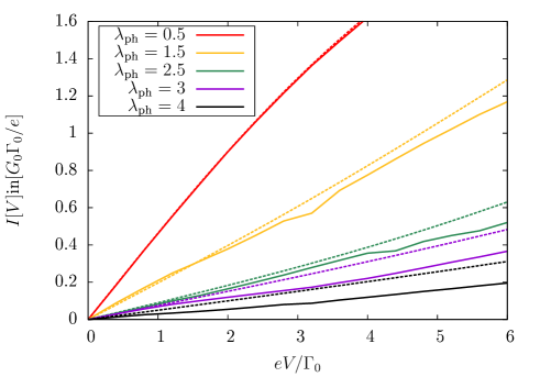
Figure 7: The evolution of $I(V)$ curves from weak to strong electron-phonon coupling for the same parameters as in fig. 4 but $T/\Gamma_{0}=1$. The straight lines are SNRG nonequilibrium results and the dashed lines are I(V) curves where we set $\rho_{d}(\omega,V)=\rho_{d}(\omega)$ in Eq. 6.

We have shown the temperature evolution of the $I(V)$ for two different moderate temperatures to make contact to the ISPI approach Hützen et al. (2012). While the ISPI is limited to large temperatures due to the discretion of the memory kernel, the SNRG can access arbitrarily low temperatures, the quantum coherence dominate the transport properties at low temperatures.

At small voltages and strong electron-phonon coupling $\lambda_{ph}/\Gamma_{0}>2.5$ the shape change of the non-equilibrium spectral function leads to a suppression of the current when the temperature is increased. The temperature dependency of the current is governed by the Fermi-functions of the lead for large voltages or small couplings $\lambda_{ph}$. We have shown that our non-equilibrium currents approach the linear response regime for small voltages in which the voltage dependency of the spectral function can be neglected. With increasing $\lambda_{ph}$, however, the validity radius of the linear response regime becomes very small.

V Acknowledgments

This paper is dedicated to the memory of Avi Schiller. He was not only a dear friend but a collaborator for over 17 years and codeveloped Anders and Schiller (2006, 2006) the non-equilibrium extension of Wilson’s numerical renormalization group which is the foundation of the scattering states approach to steady state currents applied in this paper. Furthermore, we had many fruitful discussion with Avi on the electron phonon coupling and profited a lot from his exceptionally clear written paper Eidelstein et al. (2013). We acknowledges financial support by the German-Israel Foundation through Grant No. 1035-36.14 and supercomputer support by the NIC, Forschungszentrum Jülich under project no. HHB000.

References

- Aviram and Ratner (1974) A. Aviram and M. A. Ratner, Chemical Physics Letters 29, 277 (1974).
- Chen et al. (1999) J. Chen, M. A. Reed, A. M. Rawlett, and J. M. Tour, Science 286, 1550 (1999).
- Donhauser et al. (2001) Z. J. Donhauser, B. A. Mantooth, K. F. Kelly, L. A. Bumm, J. D. Monnell, J. J. Stapleton, D. W. Price, A. M. Rawlett, D. L. Allara, J. M. Tour, and P. S. Weiss, Science 292, 2303 (2001).
- Li et al. (2003) C. Li, D. Zhang, X. Liu, S. Han, T. Tang, C. Zhou, W. Fan, J. Koehne, J. Han, M. Meyyappan, A. M. Rawlett, D. W. Price, and J. M. Tour, Appl. Phys. Lett. 82, 645 (2003).
- Galperin et al. (2007) M. Galperin, M. A. Ratner, and A. Nitzan, Journal of Physics: Condensed Matter 19, 103201 (2007).
- Kastner (1992) M. A. Kastner, Rev. Mod. Phys. 64, 849 (1992).
- Galperin et al. (2005) M. Galperin, M. A. Ratner, and A. Nitzan, Nano Letters 5, 125 (2005).
- Galperin et al. (2004) M. Galperin, M. A. Ratner, and A. Nitzan, Nano Letters 4, 1605 (2004).
- Koch and von Oppen (2005) J. Koch and F. von Oppen, Phys. Rev. Lett. 94, 206804 (2005).
- Koch et al. (2011) T. Koch, J. Loos, A. Alvermann, and H. Fehske, Phys. Rev. B 84, 125131 (2011).
- Koch et al. (2012) T. Koch, H. Fehske, and J. Loos, Physica Scripta 2012, 014039 (2012).
- Weiss et al. (2008) S. Weiss, J. Eckel, M. Thorwart, and R. Egger, Physical Review B 77, 195316 (2008).
- Hützen et al. (2012) R. Hützen, S. Weiss, M. Thorwart, and R. Egger, Phys. Rev. B 85, 121408 (2012).
- Eidelstein et al. (2013) E. Eidelstein, D. Goberman, and A. Schiller, Phys. Rev. B 87, 075319 (2013).
- Caroli et al. (1971) C. Caroli, R. Combescot, P. Nozieres, and D. Saint-James, J. Phys. C 4, 916 (1971).
- Caroli et al. (1972) C. Caroli, R. Combescot, P. Nozieres, and D. Saint-James, J. Phys. C 5, 21 (1972).
- Lang and Firsov (1962) I. G. Lang and Y. A. Firsov, JETP 16, 1301 (1962).
- Leturcq et al. (2009) R. Leturcq, C. Stampfer, K. Inderbitzin, L. Durrer, C. Hierold, E. Mariani, M. G. Schultz, F. von Oppen, and K. Ensslin, Nature Physics 5, 327 (2009).
- Wilson (1975) K. G. Wilson, Rev. Mod. Phys. 47, 773 (1975).
- Bulla et al. (2008) R. Bulla, T. A. Costi, and T. Pruschke, Rev. Mod. Phys. 80, 395 (2008).
- Hewson and Meyer (2002) A. C. Hewson and D. Meyer, J. Phys.: Condens. Matter 14, 427 (2002).
- Jovchev and Anders (2013) A. Jovchev and F. B. Anders, Phys. Rev. B 87, 195112 (2013).
- Anders (2008a) F. B. Anders, Phys. Rev. Lett. 101, 066804 (2008a).
- Schmitt and Anders (2010) S. Schmitt and F. B. Anders, Phys. Rev. B 81, 165106 (2010).
- Schmitt and Anders (2011) S. Schmitt and F. B. Anders, Phys. Rev. Lett. 107, 056801 (2011).
- Vinkler et al. (2012) Y. Vinkler, A. Schiller, and N. Andrei, Phys. Rev. B 85, 035411 (2012).
- Mahan (1981) G. Mahan, Many-Particle Physics (Plenum Press, New York, 1981).
- Hershfield (1993) S. Hershfield, Phys. Rev. Lett. 70, 2134 (1993).
- Anders and Schiller (2005) F. B. Anders and A. Schiller, Phys. Rev. Lett. 95, 196801 (2005).
- Anders and Schiller (2006) F. B. Anders and A. Schiller, Phys. Rev. B 74, 245113 (2006).
- Eidelstein et al. (2012) E. Eidelstein, A. Schiller, F. Güttge, and F. B. Anders, Phys. Rev. B 85, 075118 (2012).
- Guettge et al. (2013) F. Guettge, F. B. Anders, U. Schollwoeck, E. Eidelstein, and A. Schiller, Phys. Rev. B 87, 115115 (2013).
- Suzuki (1971) M. Suzuki, Physica 51, 277 (1971).
- Peters et al. (2006) R. Peters, T. Pruschke, and F. B. Anders, Phys. Rev. B 74, 245114 (2006).
- Anders (2008b) F. B. Anders, J. Phys.: Condens. Matter 20, 195216 (2008b).
- Meir and Wingreen (1992) Y. Meir and N. S. Wingreen, Phys. Rev. Lett. 68, 2512 (1992).
- Oguri (2007) A. Oguri, Phys. Rev. B 75, 035302 (2007).
- Schiller and Hershfield (1995) A. Schiller and S. Hershfield, Phys. Rev. B 51, 12896 (1995).