Surface Configuration in $R+\mu^{4}/R$ Gravity

Abstract

We investigate the conditions on the additional constant $\mu$ in the so-called $R+\mu^{4}/R$ theory of gravity, due to existence of different kinds of space-like surfaces in both weak field and strong field limits, and their possible correspondence to black hole event horizons. Adopting a Schwarzschild limit, we probe the behaviour of $\mu$ in different contexts of radial and radial-rotational congruence of null geodesics. We show that these cases serve as correspondents to black hole horizons in some peculiar cases of study.

keywords: $f(R)$ gravity, Black hole horizons, Null geodesic flows, Raychaudhuri equation

Department of Physics, Payame Noor University (PNU), PO BOX 19395-3697 Tehran, Iran

1 Introduction

The mathematical features of a black hole, depending on peculiar singularities in solutions of Einstein field equations, became more interesting after the concept of an Event Horizon was introduced by Finkelstein [1]. This was when he noted a null 2-dimensional hypersurface in Schwarzschild spacetime, through which light rays can pass, but they will be trapped beyond. Even though this is not the only way of defining a horizon, however it appeared to be of the most interest. Therefore since no one can interact with what is beyond a horizon, the only way that one can investigate the physics of a black hole, is to examine its horizon or strictly speaking, the space-like surface which conceals the black hole. Mostly, black holes are mathematically extrapolated from solutions of general relativity. On the other hand, a great deal of physicists’ attention have been devoted to alternatives to general relativity, specially after discovery of accelerated expansion of universe in the late of 90’s, according to the observed anomalous redshift of SNIa [2, 3]. These observations somehow led to the appearance of dark energy concepts. Moreover, the observation of galactic flat rotation curves, led to the advent of dark matter scenario [4].

However some believe that our inability to properly explain this accelerated expansion, stems from our misinterpretations of gravitation. So it seems that proposing a viable alternative to general relativity would be of benefit. However as it was stated above, the important concept of black holes should be valid in a gravitational theory. Therefore, there have been so much endeavors to obtain same results in modified theories [5].

One of the most essential alternatives to general relativity which this article is mostly devoted to a peculiar class of it, is $f(R)$ theories (introduced in the next section) and black hole physics has been also discussed in this theory (e.g. see [6, 7, 8]). Therefore it seems plausible to look for the behaviour of the so-called space-like surfaces on possible black-holes. In this paper, we are about to take care about this problem, by considering a peculiar class of $f(R)$ theories, namely the $R+\mu^{4}/R$ theory of gravity.

The paper is organized as follows: in section 2 we bring a constructive review on the $f(R)$ gravity and its special case, $R+\mu^{4}/R$ theory. In section 3, we use a weak field static solution of the theory to investigate the behaviour of null-like geodesic congruence which are passing the surfaces and discuss the possible types. Same procedure is exploited for the strong filed limit of the theory in section 4. We summarized in section 5.

2 $R+\mu^{4}/R$ Theory of Gravity

In the metric formalism, the general $f(R)$ action is written as [9]

$$S_{f(R)}=\frac{1}{2\kappa^{2}}\int\textrm{d}^{4}x\sqrt{-g}\,\,f(R)+\int\textrm{d}^{4}x\,\,\mathcal{L}_{m}\left(g_{ab,\Psi_{m}}\right),$$ (1)

where $f(R)$ is an arbitrary (analytic) function of the Ricci scalar curvature of spacetime [10] and $\mathcal{L}_{m}$ is the matter Lagrangian for perfect fluids, depending on the spacetime metric $g_{ab}$ and the matter/energy fields $\Psi_{m}$. There have been also studies on the cases in which the Ricci scalar and matter are coupled [11, 12, 13]. The standard metric variation with respect to $g_{ab}$ provides the field equations

$$f^{\prime}(R)R_{ab}-\frac{1}{2}f(R)g_{ab}-\nabla_{a}\nabla_{b}f^{\prime}(R)+g_{ab}\Box f^{\prime}(R)=\kappa^{2}T_{ab},$$ (2)

with $f^{\prime}(R)=\frac{\textrm{d}f}{\textrm{d}R}$ and $T_{ab}=-\frac{2}{\sqrt{-g}}\frac{\delta\mathcal{L}_{m}}{\delta g^{ab}}$. Evidently, for $f(R)=R$, the field equations (2) will regain the Einstein field equations of general relativity. However, the most intuitive alternative conjecture is $f(R)=R+\alpha R^{2}$, proposed by Starobinsky [14], as the first inflationary model. In this case the cosmic acceleration ends for $\alpha R^{2}<R$. Moreover, Capozziello proposed an $f(R)$ model to obtain the cosmic late-time acceleration [15], where he puts his higher order gravity model in the category of modified matter models. However in this paper, we concern about another model, where $f(R)=R\pm\mu^{2(n+1)}/R^{n}$ (in this paper we consider $n=1$). The model has been proposed in [16, 17, 18, 19]. For $R^{n+1}>>\mu^{2(n+1)}$, we have $\frac{f(R)}{R}\rightarrow 1$, so the $\mu$-dependent modification is vanished in this limit. However for $R^{n+1}<<\mu^{2(n+1)}$, we get $\frac{f(R)}{R}\approx 1\pm\mu^{2(n+1)}$; then one can expect the modification to the scalar gravity. The minus case however, appeared to be encountering several shortcomings. For example the matter instability [20], absence of the matter domination era [21, 22] and inability to satisfy local gravity constraints [23, 24, 25, 26, 27]. These problems stem from the fact that in this model, $f^{\prime\prime}(R)<0$. However for $f(R)=R+\mu^{2(n+1)}/R^{n}$, we have $f^{\prime\prime}(R)>0$ and it has been shown that in this case, the problems are vanished and the theory becomes stable [19], as well as some other models [28, 29]. Furthermore it has been proved that this model retains the matter domination era [30]. In order to be in agreement with solar system experiments, in two interesting papers [31, 32] the authors obtain static spherically symmetric solutions the case of $n=1$, i.e. for $R\pm\mu^{4}/R$ theory of gravity, in both contexts of weak and strong gravitational fields. In forthcoming sections, we consider null-like geodesic congruences in the spacetimes described by the positive part of mentioned solutions.

3 Null Flows in the Weak Field Solution of $R+\mu^{4}/R$ Gravity

The weak field static spherically symmetric solution for $R+\mu^{4}/R$ gravity in solar system is ($c=1$)

$$\textrm{d}s^{2}=-A(r)\textrm{d}t^{2}+\frac{1}{B(r)}\textrm{d}r^{2}+r^{2}\textrm{d}\Omega^{2},$$ (3)

with [31]

$$A(r)=1-\frac{2M}{r}+\frac{3}{4}\alpha(\mu r)^{4/3},$$

$$B(r)=1-\frac{2M}{r}+\alpha(\mu r)^{4/3},$$ (4)

in which $M$ is the Schwarzschild massive source and in the additional terms to Schwarzschild metric, $\alpha=(4/147)^{1/3}$. Any freely falling particle in the gravitational field described by a spacetime defined in (3), must move on a geodesic, obtained from the following geodesic equations:

$${A^{\prime}\dot{r}\dot{t}}+A\ddot{t}=0,$$

$$B^{2}\left(A\dot{t}^{2}-2r\left(\dot{\theta}^{2}+\sin^{2}(\theta)\dot{\phi}^{2}\right)\right)-B^{\prime}\dot{r}^{2}+2B\ddot{r}=0,$$

$$r\ddot{\theta}-r\sin(\theta)\cos(\theta)\dot{\phi}^{2}+{2\dot{\theta}\dot{r}}=0,$$

$${2\dot{\phi}\left(\dot{r}+r\cot(\theta)\dot{\theta}\right)}+r\ddot{\phi}=0.$$ (5)

Form now on, prime stands for $\frac{\textrm{d}}{\textrm{d}r}$ and dot for $\frac{\textrm{d}}{\textrm{d}\tau}$, with $\tau$ as the trajectory parameter. Any congruence of curves, which are obtained by integrating the above geodesic equations, form a flow of integral curves in the spacetime. Moreover, if massless particles are considered, we should also take into account the null condition $g_{ab}\dot{x}^{a}\dot{x}^{b}=0$; .i.e.

$$-AB\dot{t}^{2}+{\dot{r}^{2}}+Br^{2}\left(\dot{\theta}^{2}+\sin^{2}(\theta)\dot{\phi}^{2}\right)=0.$$ (6)

So the flow obeying (6), is indeed a null flow, consisting of for example light rays, or light flows. Now let us consider a 2-space, through which the light rays go in or go out. Either of outgoing and ingoing flows are led by a tangential null vector field, respectively $l^{a}$ and $n^{a}$. Therefore these vectors satisfy $l^{a}l_{a}=n^{a}n_{a}=0$. Now consider a 2-space defined by the metric [33]

$$h_{ab}=g_{ab}+l_{a}n_{b}+l_{b}n_{a},$$ (7)

orthogonal to both of outgoing and ingoing vectors, i.e. $h_{ab}l^{a}=h_{ab}n^{a}=0$. Hence in order to satisfy this, an additional condition $l^{a}n_{a}=-1$ is mandatory, so that ${h^{a}}_{a}=2$.

Let us define a tensor

$$X_{ab}=\nabla_{a}l_{a},$$ (8)

orthogonal to the null congruence, i.e. $X_{ab}l^{a}=X_{ab}l^{b}=0$. One can decompose $X_{ab}$ to symmetric and anti-symmetric parts

$$X_{ab}=\theta_{ab}+\omega_{ab},$$ (9)

where the symmetric part $\theta_{ab}$ itself, can be decomposed to trace and traceless parts

$$\theta_{ab}=\frac{1}{2}\,\Theta\,h_{ab}+\sigma_{ab}.$$ (10)

Inclusion in (9) and taking the trace ${X_{a}}^{a}$ yields

$${X_{a}}^{a}=\Theta=\nabla_{a}l^{a}.$$ (11)

The scalar expansion $\Theta$ is the fractional rate of change of the congruence, per unite affine parameter, in the transverse cross-sectional area described by the 2-metric $h_{ab}$. Moreover, the traceless part of (10) is defined as

$$\sigma_{ab}=\nabla_{(a}l_{b)}-\frac{\Theta}{2}h_{ab},$$ (12)

which is the symmetric shear. Also the anti-symmetric part of (9) is the anti-symmetric vorticity

$$\omega_{ab}=\nabla_{[a}l_{b]}.$$ (13)

These kinematical characteristics constitute the outstanding Raychaudhuri equation [33, 34]

$$\dot{\Theta}=-\frac{1}{2}\Theta-\sigma^{2}+\omega^{2}-R_{ab}l^{a}l^{b},$$ (14)

with $\sigma^{2}=\sigma_{ab}\sigma^{ab}$ and $\omega^{2}=\omega_{ab}\omega^{ab}$ in which $\sigma^{ab}=g^{ae}g^{bf}\sigma_{ef}$ and $\omega^{ab}=g^{ae}g^{bf}\omega_{ef}$ are obtained with respect to the background spacetime metric. The Raychaudhuri equation (14), has appeared to be a quite useful mathematical tool to investigate the focusing theorem and the concept of singularity [35, 36, 37]. To go any further, we confine our flow to move only in equatorial plane ($\theta=\pi/2$), so any tangential outgoing vector field $l^{a}$ in a sapcetime like (3) and in equatorial plane can be defined as

$$l^{a}=\left(\dot{t},\dot{r},0,\dot{\phi}\right).$$ (15)

3.1 Pure Radial Flow

In this case we consider $\phi=$const. So integrating the first in (3) results in

$$\dot{t}=\frac{E}{A},$$ (16)

where $E$, based on the definition $E=-g_{00}\dot{t}$ [38], is the positive energy of moving particles and is indeed a constant of motion. Accordingly, and using the null condition (6), we get

$$l^{a}=E\left(\frac{1}{A},-\sqrt{\frac{B}{A}},0,0\right).$$ (17)

The condition $l^{a}n_{a}=-1$ for the outgoing null vector $n^{a}$, provides

$$n^{a}=\frac{1}{2E}\left(1,\sqrt{AB},0,0\right).$$ (18)

Now let us introduce three important kinematical characteristics of affinely parameterized geodesic flows, like the ones defined by (17) and (18). In (14) we define

$$\Theta_{l}=\nabla_{a}l^{a},$$

$$\Theta_{n}=\nabla_{a}n^{a},$$ (19)

to be the scalar expansion, respectively of affinely parameterized ingoing and outgoing flows. These parameters are indeed in the 2-space $h_{ab}$, however if we are interested in what it really is, we should examine both orthogonally ingoing and outgoing flows through this 2-space, while they are propagated in the gravitational field. The expansions (3.1) for the weak field values of $R+\mu^{4}/R$ gravity, given in (3) and corresponding tangential vectors (17) and (18) are

$$\Theta_{l}=-\frac{4E}{r}\sqrt{\frac{2M-r\left(\alpha(\mu r)^{4/3}+1\right)}{8M-r\left(3\alpha(\mu r)^{4/3}+4\right)}},$$

$$\Theta_{n}=\frac{r\left(5\alpha(\mu r)^{4/3}+4\right)-4M}{2Er^{2}}\sqrt{\frac{2M-r\left(\alpha(\mu r)^{4/3}+1\right)}{8M-r\left(3\alpha(\mu r)^{4/3}+4\right)}}.$$ (20)

Here, we bring a discussion on the types of 2-surfaces which are directly extrapolated from the values in (3.1), based on the information in [39, 40, 41, 42, 43] (also for a very good review see [44]).

• For $h_{ab}$ to be a normal surface metric (like a 2-sphere in Minkowski spacetime), one must have $\Theta_{l}>0$ and $\Theta_{n}<0$.

• A trapped surface is obtained if [35] $\Theta_{l}<0$ and $\Theta_{n}<0$. Accordingly, both future directed ingoing and outgoing flows are converged at a singularity. Therefore, trapped surfaces correspond to black hole regions.

• For the outgoing flow $l^{a}$, if $\Theta_{l}=0$ and $\Theta_{n}<0$ for the ingoing flow, a marginal surface is available.

• If $\Theta_{l}\Theta_{n}<0$, then $h_{ab}$ is an un-trapped surface.

• Finally, an anti-trapped surface is obtained, when $\Theta_{l}>0$ and $\Theta_{n}>0$, which leads to diverging future directed outgoing and ingoing flows. This mean that all data will scape from the surface; representing a white hole region [45].

For the outgoing flow expansion (3.1) we always have $\Theta_{l}<0$, except for the value

$$\mu=\pm\left(\frac{2M-r}{\alpha}\right)^{3/4}\frac{1}{r^{7/4}},$$ (21)

where $\Theta_{l}=0$. Therefore we do not possess a normal surface here. Moreover, the ingoing flow expansion $\Theta_{n}$ in (3.1), vanishes for

$$\mu=\pm\left(\frac{2M-r}{\alpha}\right)^{3/4}\frac{1}{r^{7/4}}\,\,\,\,\textrm{and}\,\,\,\,=\pm\left(\frac{M-r}{5\alpha}\right)^{3/4}\frac{2\sqrt{2}}{r^{7/4}}.$$ (22)

On the other hand, we can not expect a marginal surface, since for the value in (21) for $\Theta_{l}$, we have also $\Theta_{n}=0$. However, adjacent to Schwarzschild radius $r\approx 2M$, we have

$$\Theta_{n}\approx\frac{5\alpha\mu M\sqrt[3]{2\mu M}+1}{2\sqrt{3}EM},$$ (23)

which is always positive. So according to the fact that always $\Theta_{l}<0$, then $\Theta_{l}\Theta_{n}<0$, which corresponds to an un-trapped surface. Figure 1 shows the behaviour of $\Theta_{n}$ with respect to $\mu$, near the Schwarzschild radius.

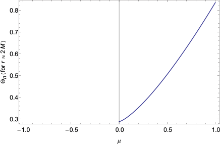
Figure 1: The behaviour of $\Theta_{n}$ with respect to $\mu$, for $r\approx 2M$ for radial flows. The plotting has been done for $E=1$, and the unit value along the $\mu$ axis is $M$. Obviously for any values of $\mu$, always $\Theta_{n}>0$.

3.2 Radial-Rotational Flow

In this case, the geodesic equations become

$$\dot{t}=\frac{E}{A},$$

$$\dot{\phi}=\frac{L}{r^{2}},$$ (24)

in which $L=g_{33}\dot{\phi}$, is the proper angular momentum of moving particles, and is another constant of motion [38]. So applying the null condition (6), the tangential vector $l^{a}$ for outgoing flow is obtained as

$$l^{a}=\left(\frac{E}{A},\sqrt{B}\sqrt{\frac{E^{2}}{A}-\frac{L^{2}}{r^{2}}},0,\frac{L}{r^{2}}\right).$$ (25)

Accordingly, the condition $l^{a}n_{a}=-1$, may result in the following for the null ingoing vector:

$$n^{a}=\frac{r^{2}}{L^{2}A}\left(E(L+1)-\sqrt{(2L+1)A}\sqrt{\frac{E^{2}}{A}-\frac{L^{2}}{r^{2}}},\,\,\,\,(L+1)A\sqrt{B}\sqrt{\frac{E^{2}}{A}-\frac{L^{2}}{r^{2}}}-\sqrt{E^{2}(2L+1)AB},\,\,\,\,\,\,\,\,0,\,\,\,\,1\right).$$ (26)

Therefore the outgoing expansion would be

$$\Theta_{l}=\frac{\sqrt{-\frac{2M}{r}+\alpha(\mu r)^{4/3}+1}\left[8E^{2}r^{3}+L^{2}\left(4M-r\left(5\alpha(\mu r)^{4/3}+4\right)\right)\right]}{r^{2}\sqrt{r\left(3\alpha(\mu r)^{4/3}+4\right)-8M}\sqrt{4E^{2}r^{3}+L^{2}\left(8M-r\left(3\alpha(\mu r)^{4/3}+4\right)\right)}}$$ (27)

The result for $\Theta_{n}$ becomes rather complicated, however once again we can plot the Schwarzschild limit of both $\Theta_{l}$ and $\Theta_{n}$. Figure 2 shows these values which has been plotted in terms of $\mu$, for different values of $E$ and $L$.

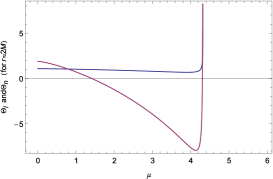
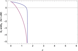
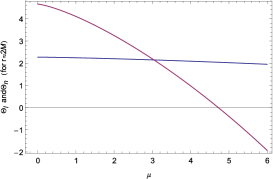
a)  b)  c)

Figure 2: The behaviour of $\Theta_{l}$ (blue line) and $\Theta_{n}$ with respect to $\mu$, for $r\approx 2M$ for radial-rotational congruence. The plotting has been done for (a) $E=1$ and $L=1$, (b) $E=1$ and $L=2$ and (c) $E=2$ and $L=1$. the unit value along the $\mu$ axis is $M$.

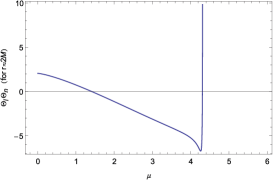
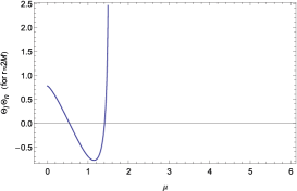
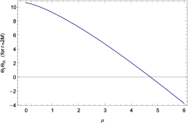
a)  b)  c)

Figure 3: The behaviour of $\Theta_{l}\Theta_{n}$ with respect to $\mu$, for $r\approx 2M$ for radial-rotational. The plotting has been done for (a) $E=1$ and $L=1$, (b) $E=1$ and $L=2$ and (c) $E=2$ and $L=1$. the unit value along the $\mu$ axis is $M$. As it is seen, these may include un-trapped, trapped, anti-trapped and marginal surfaces.

The expansions do not have real values for $\mu<0$. One can see that at some points we encounter both $\Theta_{l}<0$ and $\Theta_{n}<0$ which corresponds to trapped surfaces for $h_{ab}$, or black hole event horizons. However according to figure 2, one can see that the values of $\Theta_{l}\Theta_{n}$ are somewhere negative and somewhere positive. This can provide that we have un-trapped surfaces as well as trapped and anti-trapped ones. Moreover, for $\Theta_{l}\Theta_{n}=0$ in figure 3, marginal surfaces may be available.

4 Strong Field Counterpart

Given in [32] and corresponding to (3), the strong field static solution to $R+\mu^{4}/R$ gravity is

$$A(r)=-\frac{1}{8}3\sqrt[3]{\frac{4}{3}}(2\mu M)^{4/3}\left(\frac{r}{2M}-1\right)^{2/3}-\frac{2M}{r}+1,$$

$$B(r)=\frac{1}{\frac{1}{8}\sqrt[3]{\frac{4}{3}}(2\mu M)^{4/3}\left(\frac{r}{2M}-1\right)^{2/3}-\frac{2M}{r}+1}.$$ (28)

Accordingly, the value of $\Theta_{l}\Theta_{n}$ in the Schwarzschild limit (with $M=1$) becomes

$$\Theta_{l}\Theta_{n}\approx-\frac{2\left(6^{2/3}\mu^{8/3}-2\sqrt[3]{2}\mu^{4/3}\sqrt[3]{r-2}+4\sqrt[3]{3}(r-2)^{2/3}\right)\left(6^{2/3}\mu^{8/3}-2\sqrt[3]{2}\mu^{4/3}\sqrt[3]{r-2}+3\sqrt[3]{3}\mu^{4}(r-2)^{2/3}+4\sqrt[3]{3}(r-2)^{2/3}\right)}{3\ 3^{2/3}\mu^{8}(r-2)^{4/3}},$$ (29)

which does not depend on the energy $E$. One can plot while $r$ is still changing in the desired domain (see figure 4). Apparently for all values of $\mu$ near $r=2M$, always $\Theta_{l}\Theta_{n}<0$. So we possess un-trapped surfaces.

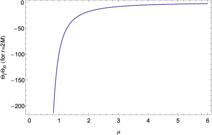
Figure 4: The behaviour of $\Theta_{l}\Theta_{n}$ with respect to $\mu$, for $r\approx 2M$ in strong fields for radial flows. The plotting has been done $r=2.1$ the unit value along the $\mu$ axis is $M$.

If radial-rotational flows are considered, the values of $\Theta_{l}\Theta_{n}$ form a curve like figure 4 (see figure 5), however for very larger values. It turns out that these values are all negative, therefore once again we encounter un-trapped surfaces.

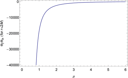
Figure 5: The behaviour of $\Theta_{l}\Theta_{n}$ with respect to $\mu$, for $r\approx 2M$ in strong fields for radial-rotational flows. The plotting has been done for $E=1$, $L=1$ and $r=2.1$ the unit value along the $\mu$ axis is $M$.

4.1 A Note on the Initial Values for Radial-Rotational Flows

If the particles are commencing motion (at $\tau=0$) form a initial radial point $r_{0}$, where $r_{0}=r(\tau)|_{\tau=0}$, and with temporal initial velocity $u_{t}=\dot{t}|_{\tau=0}$, radial initial velocity $u_{r}=\dot{r}|_{\tau=0}$ and initial angular velocity $\omega_{0}=\dot{\phi}|_{\tau=0}$, then the values of energy $E$ and angular momentum $L$ in (3.2) can be rewritten as

$$E=u_{t}A_{0},$$

$$L=\omega_{0}{r_{0}}^{2},$$ (30)

where $A_{0}=A(r_{0})$. Now if we consider the particles to be released from a circular orbit of radius $r_{0}$, then we can ignore $u_{r}$, since by the time the particles are released ($\tau=0$), they are at a constant position $r=r_{0}$ on a circle. Hence, the corresponding null condition (6) at $\tau=0$ gives

$${\omega_{0}}^{2}=\frac{A_{0}}{{r_{0}}^{2}}u_{t}^{2}.$$ (31)

Also from (25) and (4.1) we have

$$\sqrt{B_{0}}\sqrt{\frac{{A_{0}}^{2}u_{t}^{2}}{A_{0}}-(r_{0}\omega_{0})^{2}}=0.$$ (32)

Therefore using (31), one can obtain

$$u_{t}=\pm\frac{r_{0}}{\sqrt{A_{0}}}.$$ (33)

So both constants of motion, can be expressed in terms of the initial radius of release $r_{0}$.

5 Conclusion

In this paper we investigated the 2-dimensional cross-sectional surfaces of exterior geometries of $R+\mu^{4}/R$ theory of gravity, through which the null congruence of geodesic integral curves (null flows) can pass. We pursued both weak field and strong field limits. Our method was based on inspecting the expansion of the outgoing and ingoing flows, in which the signs of these expansions were crucial to the type of the mentioned surface. According to different types of motion, we obtained different types of surfaces, including black hole horizons (trapped surfaces). However, this type of surface was rather rare, since most of the types included un-trapped surfaces. Foe purely radial congruence in weak field limit, we discovered that no matter $\mu$ is positive or negative, we do not encounter a black hole, since always $\Theta_{l}\Theta_{n}<0$. Once radial-rotational flows are assumed, then one can observe that in order to have real values, $\mu>0$ is mandatory. Regarding its evolution, these positive values can affect $\Theta_{l}\Theta_{n}$ in a way that in terms of $\mu$, the surface may evolve from a trapped (black hole) or anti-trapped (white hole) surface, to a marginal and eventually to an un-trapped surface. This can be seen in all three cases of figure 3. However,for evolving surfaces in the strong field limit, in both cases of radial and radial-rotational congruence and regardless of numerical values, $\Theta_{l}\Theta_{n}$, is always negative. This means that the cosmological term $\mu$ imposes a rather reach effect on the gravitational attraction, enforcing $h_{ab}$ to define an un-trapped surface. In this case, the extra term $\mu$, as a cosmological background on Schwarzschild geometry, causes some sort of repelling force, which cancels out the possibility of a gravitational collapse. So, it seems that to find possible $f(R)$ black holes in $R+\mu^{4}/R$ gravity, one must take only its weak field limit geometry.

Acknowledgements      We would like to thank the referee for useful comments, which helped us improve the presentation of the paper.

References

- [1] D. Finkelstein: Phys. Rev., 110, (4), 965-967 (1958)
- [2] A.G. Riess, et al.: Astron. J. 116, 1009 (1998)
- [3] S. Perlmutter, et al.: Astrophys. J. 517, 565 (1999)
- [4] M. Persic, P. Salucci, F. Stel: Mon. Not.Roy. Astron. Soc. 281, 27 (1996)
- [5] A. de la Cruz-Dombriz, A. Dobado, A.L. Maroto: Journal of Physics: Conference Series, 229, 012033 (2010)
- [6] A. de la Cruz-Dombriz, A. Dobado, A.L. Maroto: Phys. Rev. D, 80, 124011 (2009)
- [7] Y.S. Myung, T. Moon, E.J. Son: Phys. Rev. D, 83, 124009 (2011)
- [8] A.M. Nzioki, R. Goswami, P.K.S. Dunsby: arXiv:1408.0152v2 (2014)
- [9] T.P. Sotiriou, V. Faraoni: Rev. Mod. Phys., 82, January-March (2010)
- [10] S. Capozziello, M. Francaviglia: Gen. Rel. Grav, 40, 357-420 (2008)
- [11] O. Bertolami, C.G Boehmer, T. Harko, F.S.N. Lobo: Phys. Rev. D, 75, 104016 (2007)
- [12] O. Bertolami, J. Paramos: Phys. Rev. D, 77, 084018 (2008)
- [13] V. Faraoni: Phys. Rev. D, 80, 124040 (2009)
- [14] A.A. Starobinsky: Phys. Lett. B, 91, 99 (1980)
- [15] S. Capozziello: Int. J. Mod. Phys. D, 11, 483 (2002)
- [16] S. Capozziello, S. Carloni, A. Troisi: Recent Res. Dev. Astron. Astrophys., 1, 625 (2003)
- [17] S. Capozziello, V.F. Cardone, S. Carloni: A. Troisi, Int. J. Mod. Phys. D, 12, 1969 (2003)
- [18] S.M. Carroll, V. Duvvuri, M. Trodden, M.S. Turner: Phys. Rev. D, 70, 043528 (2004)
- [19] S. Nojiri and S. D. Odintsov, Phys. Rev. D, 68, 123512 (2003)
- [20] A.D. Dolgov, M. Kawasaki: Phys. Lett. B, 573, 1 (2003)
- [21] L. Amendola, D. Polarski, S. Tsujikawa: Phys. Rev. Lett., 98, 131302 (2007)
- [22] L. Amendola, D. Polarski, S. Tsujikawa: Int. J. Mod. Phys. D, 16, 1555 (2007)
- [23] T. Chiba: Phys. Lett. B, 575, 1 (2003)
- [24] G.J. Olmo: Phys. Rev. Lett., 95, 261102 (2005)
- [25] G.J. Olmo: Phys. Rev. D, 72, 083505 (2005)
- [26] I. Navarro, K. Van Acoleyen: JCAP 0702, 022 (2007)
- [27] T. Chiba, T.L. Smith, A.L. Erickcek: Phys. Rev. D, 75, 124014 (2007)
- [28] S. Nojiri, S.D. Odintsov: Phys. Lett. B, 657, 238 (2007)
- [29] S. Nojiri, S.D. Odintsov: Phys. Rev. D, 77, 026007 (2008)
- [30] I. Sawicki, W. Hu: Phys. Rev. D, 75, 127502 (2007)
- [31] K. Saaidi, A. Vajdi, A. Aghamohammadi: Gen. Relativ. Gravit., 42, 2421-2429 (2010)
- [32] K. Saaidi, A. Vajdi, S.W. Rabiei, A. Aghamohammadi, H. Sheikhahmadi: Astrophys. Space. Sci., 337, 739-745 (2012)
- [33] E. Poisson: A Relativist s Toolkit: The Mathematics of Black-Hole Mechanics, Cambridge University Press, Cambridge, UK (2004)
- [34] A.K. Raychaudhuri: Phys. Rev., 98, 1123 (1955)
- [35] R. Penrose: Phys. Rev. Lett., 14, 57 (1965)
- [36] S.W. Hawking, R. Penrose: Proc. R. Soc. A, 314, 529 (1970)
- [37] S.W. Hawking, G.F.R Ellis: The Large Scale Structure of Space-Time, Cambridge University Press, Cambridge, UK (1973)
- [38] C.W. Misner, K.S. Thorne, J.A. Wheeler: Gravitation, New York Press (1973)
- [39] I. Booth: Can. J. Phys., 83, 1073-1099 (2005)
- [40] A.B. Nielsen: Gen. Relativ. Gravit., 41, 1539-1584 (2009)
- [41] E. Gourghoulhon, J.L. Jaramillo: New Astron. Rev., 51, 791-798 (2008)
- [42] A. Ashtekar, G.J. Galloway: Adv. Theor. Math. Phys., 9, 1-30 (2005)
- [43] I. Booth, L. Brits, J.A. Gonzalez, V. van den Broeck: Class. Quant. Grav., 23, 413 (2006)
- [44] V. Faraoni: Galaxies, 1, 114-179 (2013)
- [45] S.M. Carroll: Spacetime and Geometry, Addison Wesley, ISBN 0-8053-8732-3 (2004)