Rotating a Rashba-coupled Fermi gas in two dimensions

Abstract

We analyze the interplay of adiabatic rotation and Rashba spin-orbit coupling on the BCS-BEC evolution of a harmonically-trapped Fermi gas in two dimensions under the assumption that vortices are not excited. First, by taking the trapping potential into account via both the semi-classical and exact quantum-mechanical approaches, we firmly establish the parameter regime where the non-interacting gas forms a ring-shaped annulus. Then, by taking the interactions into account via the BCS mean-field approximation, we study the pair-breaking mechanism that is induced by rotation, i.e., the Coriolis effects. In particular, we show that the interplay allows for the possibility of creating either an isolated annulus of rigidly-rotating normal particles that is disconnected from the central core of non-rotating superfluid pairs or an intermediate mediator phase where the superfluid pairs and normal particles coexist as a partially-rotating gapless superfluid.

I Introduction

The quantum behavior of superfluids is most evident when they are placed in a rotating container. While a slow rotation may lead to the appearance of quantized vortices or quenching of the moment of inertia Abo2001 ; Zwerlein2005 , rapidly-rotating systems may exhibit integer and fractional quantum-Hall physics Ho2000 ; Cooper2001 ; Fischer2003 ; Baranov2005 . On the other hand, the Rashba spin-orbit coupling (SOC) involves an intrinsic angular momentum, caused by coupling the particle’s spin to its momentum, and it has become one of the key themes in modern condensed-matter and atomic physics, playing a central role for systems such as topological insulators and superconductors Hasan2010 ; Qi2011 , quantum spin-Hall systems Sinova2004 , and spintronics applications Zutic2004 .

Hence, the interplay between rotation and SOC is expected to pave the way for novel quantum phenomena, and recent realizations of SOC in atomic gases have already set the stage for such a task in a highly-controllable setting Lin2011 ; Zhang2012 ; Wang2012 ; Cheuk2012 ; Qu2013 ; Goldman2014 ; Olson2014 ; Jimenez-Garcia2015 ; Huang2015 . While only the NIST-type SOC has so far been achieved, there also exist various proposals on how to create a purely Rashba SOC Ruseckas2005 ; Campbell2011 ; Xu2012 , the possibility of which has stimulated numerous theoretical studies on Rashba-Fermi gases in three Vyasanakere2011 ; Jiang2001 ; Yu2011 ; Gong2011 ; Iskin2011 ; Yi2011 ; Zhou2012 ; Liao2012 ; Han2012 as well as two He2012 ; Gong2012 ; Yang2012 ; Takei2012 ; Ambrosetti2014 ; Zhang2013 ; Iskin2013 ; Cao2014 dimensions. These works have revealed a plethora of intriguing phenomena, including topological superfluids, Majorana modes, spin textures, skyrmions, etc., which may soon be observed given the recent advances in producing a two-dimensional Fermi gas Huang2015 ; Martiyanov2010 ; Dyke2011 ; Frohlich2011 ; Feld2011 ; Sommer2012 ; Ries2015 .

In this paper, we study the cooperation of adiabatic rotation and Rashba SOC on the ground-state phases of a trapped Fermi gas assuming that vortices are not excited. Adiabaticity requires that the rotation is introduced slowly to the system. In particular the rate of change of rotation frequency should be much smaller than the quasiparticle excitation frequency for vortex creation. In the absence of a SOC, effects of rotation on three-dimensional Fermi gases have previously been studied under this assumption at unitarity using the quantum Monte Carlo equations of state together with the local-density approximation (LDA) Bausmerth2008a ; Bausmerth2008 , and throughout the BCS-BEC evolution using the BCS mean-field approximation together both with LDA Urban2008 and the Bogoliubov-de Gennes approach Iskin2009 . These works have shown that, by breaking some of the superfluid (SF) pairs via the Coriolis effects, rotation gives rise to a phase separation between a non-rotating SF core at the center and a rigidly-rotating normal (N) particles at the outer edge Bausmerth2008a ; Bausmerth2008 , with a partially-rotating gapless SF (gSF) region in between where the SF pairs and N particles coexist together Urban2008 ; Iskin2009 . Since the effects of the Coriolis force on a neutral particle in the rotating frame are similar to those of the Lorentz force on a charged particle in a magnetic field, current advances in simulating artificial fields with ultracold atoms opens alternative ways of effectively realizing a rotating Fermi gas with SOC. In addition, more recent works have confirmed that pair-breaking scenario is energetically more favored against vortex formation in a sizeable parameter regime Warringa2011 ; Warringa2012 , and experimental schemes for realizing a rotating spin-orbit coupled system are described in  Radic2011 .

Figure 1: (Color online) Cartoon pictures showing that (a) the whole gas is a SF in the absence of rotation, (b) an intermediate gSF phase (where the SF and N particles coexist) emerges due to pair-breaking induced by sufficiently high rotations, and (c) N particles is disconnected from the central SF core due to SOC at sufficiently high rotations.

In the presence of a Rashba SOC, we first take the harmonic confinement into account via both the semi-classical LDA and exact approaches, and find the parameter regime where the non-interacting gas forms a ring-shaped annulus. Neither rotation nor SOC alone can deplete the central density to zero no matter how fast the rotation or large SOC is, and the formation of such an intriguing annulus requires them both simultaneously. Then, we take the interactions into account via the BCS mean-field, and analyze the pair-breaking mechanism in the entire BCS-BEC evolution. In particular, we show that the cooperation of rotation and SOC allows for the possibility of creating either an isolated annulus of N particles that is disconnected from the central SF core or separated from it by an intermediate gSF phase as sketched in Fig. 1. We also construct phase diagrams showing the very first emergence of an N phase and the complete destruction of the central SF core.

II Theoretical Formalism

To obtain these results, we use the following Hamiltonian density in the rotating frame

$$H(\mathbf{r})=\psi^{\dagger}(\mathbf{r})\left[\frac{\mathbf{p}^{2}}{2M}+V(r)-\mu-\Omega L_{z}+\alpha\mathbf{p}\cdot\vec{\mathbf{\sigma}}\right]\psi(\mathbf{r})$$

$$+\Delta(\boldsymbol{r})\psi_{\uparrow}^{\dagger}(\mathbf{r})\psi_{\downarrow}^{\dagger}(\mathbf{r})+\Delta^{*}(\boldsymbol{r})\psi_{\downarrow}(\mathbf{r})\psi_{\uparrow}(\mathbf{r})+\frac{|\Delta(\boldsymbol{r})|^{2}}{g},$$ (1)

where $\psi^{\dagger}=(\psi_{\uparrow}^{\dagger},\psi_{\downarrow}^{\dagger})$ denotes the field operators, $\mathbf{p}=-i\mathbf{\nabla}$ is the linear-momentum operator with $\hbar=1$, $V(r)=M\omega^{2}r^{2}/2$ is the trapping potential, $\mu$ is the chemical potential, $0\leq\Omega<\omega$ is the rotation frequency, $L_{z}$ is the $z$-projection of the angular-momentum operator $\mathbf{L}=\mathbf{r}\times\mathbf{p}$, $\alpha\geq 0$ is the strength of the Rashba coupling, $\vec{\mathbf{\sigma}}=(\sigma_{x},\sigma_{y})$ is a vector of Pauli spin matrices, and $\Delta(\boldsymbol{r})=g\langle\psi_{\uparrow}(\mathbf{r})\psi_{\downarrow}(\mathbf{r})\rangle$ is the mean-field SF order parameter with $g\geq 0$ being the strength of attractive interactions and $\langle\cdots\rangle$ the thermal average. Within the semi-classical LDA, the local Hamiltonian can be written as $H_{\mathrm{loc}}=(1/2)\sum_{\mathbf{k}}\psi_{\mathbf{k}}^{\dagger}H_{\mathbf{k}}\psi_{\mathbf{k}}+C,$ where the matrix

$$H_{\mathbf{k}}\!\!=\!\!\begin{pmatrix}\!\xi_{\mathbf{k}}-\Omega L_{\mathbf{k}}&S_{\mathbf{k}}&0&\Delta\\ S_{\mathbf{k}}^{*}&\!\!\xi_{\mathbf{k}}-\Omega L_{\mathbf{k}}&-\Delta&0\\ 0&-\Delta^{*}&\!\!\!-\xi_{\mathbf{k}}-\Omega L_{\mathbf{k}}&S_{\mathbf{k}}^{*}\\ \Delta^{*}&0&S_{\mathbf{k}}&\!\!\!-\xi_{\mathbf{k}}-\Omega L_{\mathbf{k}}\end{pmatrix}$$ (2)

governs the dynamics. The index $\mathbf{r}$ is dropped here and throughout for notational simplicity. In momentum space, $\psi_{\mathbf{k}}^{\dagger}=(a_{\mathbf{k}\uparrow}^{\dagger},a_{\mathbf{k}\downarrow}^{\dagger},a_{\mathbf{-k}\uparrow},a_{\mathbf{-k}\downarrow})$ and $a_{\mathbf{k},\sigma}$ ($a_{\mathbf{k},\sigma}^{{\dagger}}$) annihilates (creates) a $\sigma$ fermion with momentum $\mathbf{k}=(k_{x},k_{y})$. The free-particle dispersion relative to the local chemical potential $\mu_{\mathbf{r}}=\mu-V(r)$ is $\xi_{\mathbf{k}}=\epsilon_{\mathbf{k}}-\mu_{\mathbf{r}}$ with $\epsilon_{\mathbf{k}}=k^{2}/(2M)$. The rotation enters via $\Omega L_{\mathbf{k}}=\mathbf{v}(\mathbf{r})\cdot\mathbf{k}$ with the velocity $\mathbf{v}(\mathbf{r})=\Omega\mathbf{\hat{z}}\times\mathbf{r}$, $S_{\mathbf{k}}=\alpha(k_{x}-ik_{y})$ is the SOC term, $\Delta=g\sum_{\mathbf{k}}\langle a_{\mathbf{k}\uparrow}a_{-\mathbf{k}\downarrow}\rangle$ denotes the SF order parameter, and $C=\sum_{\mathbf{k}}(\xi_{\mathbf{k}}+\Omega L_{\mathbf{k}})+|\Delta|^{2}/g$ is a constant.

We diagonalize Eq. (2) and express $H_{\mathrm{loc}}=C+\sum_{\mathbf{k}s}(E_{\mathbf{k}s}\gamma_{\mathbf{k}s}^{{\dagger}}\gamma_{\mathbf{k}s}-E_{\mathbf{k}s}/2),$ where $\gamma_{\mathbf{k}s}^{{\dagger}}$ ($\gamma_{\mathbf{k}s}$) creates (annihilates) a quasiparticle with helicity $s=\pm$ and energy $E_{\mathbf{k}s}=\sqrt{(\xi_{\mathbf{k}}+s\alpha k)^{2}+|\Delta|^{2}}-\Omega L_{\mathbf{k}}.$ Thus, the thermodynamic potential $G=-(1/\beta)\mathrm{Tr}(\ln e^{-\beta H_{\mathrm{loc}}}),$ where $\beta=1/(k_{B}T)$ with $k_{B}$ the Boltzmann constant and $T$ the temperature, can be written as $G=C+\sum_{\mathbf{k}s}[E_{\mathbf{k}s}f(E_{\mathbf{k}s})-E_{\mathbf{k}s}/2]$ with the Fermi function $f(x)=1/(e^{\beta x}+1)$. Setting $\partial G/\partial|\Delta|=0$ and using $n(\mathbf{r})=-(1/A)\partial G/\partial\mu_{\mathbf{r}}$ for the local particle density in area $A$, we finally obtain the local self-consistency equations

$$\frac{1}{g} =\frac{1}{4}\sum_{\mathbf{k}s}\frac{1}{E_{\mathbf{k}s}+\Omega L_{\mathbf{k}}}\tanh(\beta E_{\mathbf{k}s}/2),$$ (3)

$$n(\mathbf{r}) =\frac{1}{2A}\sum_{\mathbf{k}s}\left[1-\frac{\xi_{\mathbf{k}}+s\alpha k}{E_{\mathbf{k}s}+\Omega L_{\mathbf{k}}}\tanh(\beta E_{\mathbf{k}s}/2)\right],$$ (4)

such that the total number of particles is given by $N=\int d\mathbf{r}n(\mathbf{r})$. These equations are the generalizations of the usual BCS expressions to the case of rotation and SOC, and it is a standard practice to substitute the two-body binding energy in vacuum $E_{b}\geq 0$ for $g$ via the relation $1/g=\sum_{\textbf{k}}1/(2\epsilon_{\textbf{k}}+E_{b})$ in the cold-atom context. While a non-zero (vanishing) $\Delta$ is a characteristic of SF (N) phase in general, we also use the mass-current density $\mathbf{J}=(J_{x},J_{y})$ flowing in the azimuthal direction, where

$$(J_{x},J_{y}) =\frac{1}{A}\sum_{\mathbf{k}}\left[n_{\mathbf{k}}\mathbf{k}+2M\alpha\left(\Re\{p_{\mathbf{k}}\},\Im\{p_{\mathbf{k}}\}\right)\right],$$ (5)

to further characterize the gSF phase. Here, $n_{\mathbf{k}}=\langle a^{{\dagger}}_{\mathbf{k}\uparrow}a_{\mathbf{k}\uparrow}\rangle+\langle a^{{\dagger}}_{\mathbf{k}\downarrow}a_{\mathbf{k}\downarrow}\rangle$ is the momentum distribution given by the summand of Eq. (4), $\Re$ and $\Im$ denote the real and imaginary parts and $p_{\mathbf{k}}=\langle a^{{\dagger}}_{\mathbf{k}\uparrow}a_{\mathbf{k}\downarrow}\rangle.$ Let us first set $\Delta=0$ and $T=0$, and analyze the non-interacting ground state.

III Non-interacting Problem

In the absence of both rotation and SOC, the non-interacting gas has the shape of a disc with its density $n(r)$ decreasing parabolically as a function of $r$, until to the edge of the system given by the Thomas-Fermi radius $R_{F}=\sqrt{2E_{F}/(M\omega^{2})}$, where $E_{F}=k_{F}^{2}/(2M)=\omega\sqrt{N}$ is the Fermi energy. In the presence of rotation only, while the gas retains its overall parabolic density, some of the the particles are expelled from the center of the trap due to the centrifugal effects, and the edge moves to $\widetilde{R}_{F}=R_{F}/(1-\Omega^{2}/\omega^{2})^{1/4}$. However, in the presence of SOC only, $n(r)$ tends to increase at the center and the gas shrinks due to the increased low-energy density of states. Therefore, $\Omega\neq 0$ and $\alpha\neq 0$ have counteracting effects on $n(r)$ in general. In addition, since $\Omega\neq 0$ causes an asymmetry in the local $\mathbf{k}$ space and $\alpha\neq 0$ shifts its dispersion minima from $\mathbf{k}=\mathbf{0}$ to $\mathbf{k}\neq\mathbf{0}$, their interplay is expected to give rise to a much richer physics even in the non-interacting limit. For instance, setting $\Delta=0$ in Eq. (4), and solving for $n(r)=0$, we find an analytic expression for the edge(s) of the gas given by

$$R_{O,I}^{0}=R_{F}\frac{\omega\Omega\alpha\pm\omega\sqrt{\alpha^{2}\omega^{2}+2\mu(\omega^{2}-\Omega^{2})/M}}{k_{F}(\omega^{2}-\Omega^{2})/M},$$ (6)

where $R_{O}^{0}$ ($R_{I}^{0}$) is the radius of the outer (inner) edge. Note that while $R_{O}^{0}$ is positive and exists for all parameters as long as $\Omega<\omega$, a positive $R_{I}^{0}$ is possible only for the parameter regimes where $\alpha^{2}+2\mu/M<0$. While the gas has the usual shape of a disc with $n(r)\neq 0$ for $0\leq r<R_{O}^{0}$ when $\alpha^{2}>-2\mu/M$, otherwise it has the shape of a ring with $n(r)\neq 0$ in the radial interval $R_{I}^{0}<r<R_{O}^{0}$.

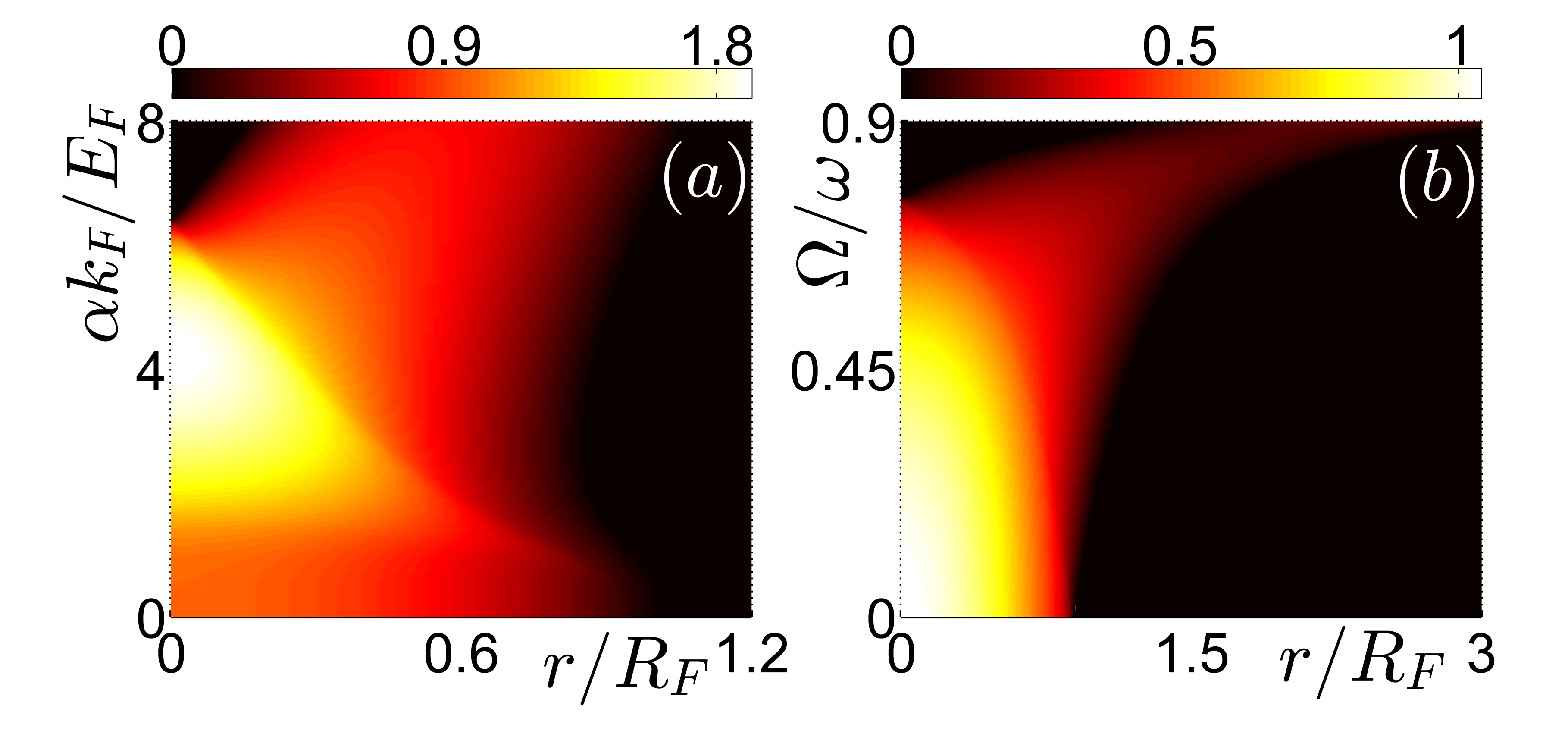
Figure 2: (Color online) Non-interacting $n(r)$ profiles are shown as a function of (a) $\alpha$ for $\Omega=0.15\omega$, and (b) $\Omega$ for $\alpha=1E_{F}/k_{F}$. The gas eventually forms a ring-shaped annulus in both figures.

The formation of such an annulus can also be illustrated by solving $n(r)$ directly from Eq. (4), which we present in Fig. 2. As shown in Fig. 2(a), while increasing $\alpha$ initially increases $n(r)$ near the central region due to the increase in the low-energy density of states, the $\mathbf{k}\neq\mathbf{0}$ states gain further energy through their angular momentum in the rotating frame, and $n(r)$ decreases dramatically away from the center as $\alpha$ increases further. As the critical condition is approached, the latter effect gradually dominates causing central density to decrease as the gas continues to expand, and $n(0)$ eventually vanishes beyond $\alpha=\sqrt{-2\mu/M}$. We also see a similar behavior in Fig. 2(b), where increasing $\Omega$ is shown to deplete $n(0)$ to zero once the critical condition is satisfied. This happens at faster $\Omega$ for smaller $\alpha$ and vice versa. In contrast to increasing $\alpha$, however, increasing $\Omega$ not only decreases $n(0)$ but also expands the gas monotonically. It is important to emphasize here that neither rotation nor SOC alone can deplete $n(0)$ to zero no matter how fast $\Omega$ or large $\alpha$ is, and the formation of an annulus requires them both simultaneously.

In the non-interacting limit, we benchmark our semi-classical results with those of exact quantum-mechanical treatment and find an excellent agreement between the two for all parameters including the fast $\Omega$ and/or large $\alpha$ limits. The details of this comparison are given in Appendix A. Motivated by this success, next we apply the LDA formalism to the entire BCS-BEC evolution at $T=0$.

IV Interacting Problem

In the absence of both rotation and SOC, the superfluid persists with $\Delta\neq 0$ as long as $n(r)\neq 0$, and therefore, the entire system is a disc-shaped gapped SF with its edge located at $R_{O}=R_{F}$ no matter how strong or weak $E_{b}$ is, which only happens in two dimensions. In the presence of an adiabatic rotation, since vortices are assumed not to be excited in the system and the gapped SF can not carry the angular momentum, some of the SF pairs must eventually break by the centrifugal effects, i.e., via the broken time-reversal symmetry, giving rise to gSF and N regions in the trap. In this paper, we distinguish gSF from SF by checking whether $J$ is non-zero or not, or equivalently whether $E_{\mathbf{k}s}$ has negative regions in $\mathbf{k}$ space or not. In addition, while both gSF and N phases have $J\neq 0$, only the N region rotates rigidly as a whole with $J=Mn(r)\Omega r$.

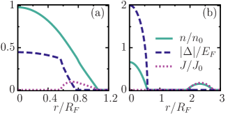
Figure 3: (Color online) Typical profiles showing (a) a partially-rotating gSF region, and (b) a vacuum seperating the non-rotating SF pairs from the rigidly-rotating N particles. Here, $E_{b}=0.1E_{F},\alpha=0.8E_{F}/k_{F}$ and $\Omega=0.3\omega$ in (a), and $E_{b}=1E_{F},\alpha=7E_{F}/k_{F}$ and $\Omega=0.5\omega$ in (b), where $n_{0}=k_{F}^{2}/(2\pi)$ and $J_{0}=Mn_{0}\omega R_{F}$.

When $\alpha=0$, the robustness of the SF pairs against rotation depends on $E_{b}$ and $\Omega$ in such a way that there is no pair breaking when $\Omega$ is sufficiently slow for a given $E_{b}$. Therefore, $n(r)$, $\Delta$ and $\mu$ are not affected by rotation as long as $\Omega<\Omega_{c}$, and the entire system is again a disc-shaped SF with its edge located at $R_{O}=R_{F}$. We determine $\Omega_{c}$ by noting that when the first broken pair emerges as N particles at the edge of the gas then its radius must coincide with the Thomas-Fermi radius of the non-rotating gas with the same $\mu$, i.e., $R_{O}^{0}(\alpha\to 0,\Omega\to\Omega_{c})=R_{F},$ leading to $\Omega_{c}=\omega\sqrt{E_{b}/(2E_{F})}$. Since $\Omega<\omega$ has a physical upper bound in order not to loose the particles from the harmonic trap, the SF pairs are perfectly robust against rotation for $E_{b}>2E_{F}$ in the $\alpha\to 0$ limit. When $\Omega>\Omega_{c}$, the trap profile in general consists of three distinct regions: while the central (outer) core (wing) is solely occupied by paired (unpaired) SF (N) particles, the SF pairs and N particles coexist in the middle as a result of which the gSF emerges as an intermediate phase around the SF-N interface. We note that even though the SF core shrinks monotonically and gives way to N phase with increasing $\Omega$, it still survives in the $\Omega\to\omega$ limit.

The preceding description still holds when $\alpha\neq 0$ but small, and we illustrate a typical trap profile in Fig. 3(a), where a small gSF region is clearly visible at the SF-N interface. Similar to the $\alpha=0$ case, the critical rotation frequency for the emergence of N particles can be determined from $R_{O}^{0}(\alpha,\Omega_{c})=R_{O}(\alpha,\Omega=0).$ Away from the small-$\alpha$ limit, however, we find a very intriguing situation provided that $\alpha^{2}<-2\mu/M$. For instance, a typical trap profile for this case is shown in Fig. 3(b), where the N particles form an isolated annulus that is completely disconnected from the central SF core without a gSF region in between. The $\Omega_{c}$ threshold for the emergence of an isolated N phase can again be determined from $R_{O}^{0}(\alpha,\Omega_{c})>R_{O}(\alpha,\Omega=0)$.

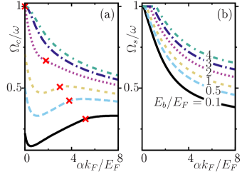
Figure 4: (Color online) Critical $\Omega$ curves are shown for (a) the emergence of an N phase, and (b) the depletion of the SF core. Beyond the (red) cross marks in (a), the N particles form an isolated annulus that is disconnected from the central SF core without a gSF region in between.

By repeating this analysis numerous times for a wide range of parameters, we construct the phase diagram of the system based on the very first emergence of N particles with increasing $\Omega$. The diagram shown in Fig. 4(a) is one of our primary results in this paper and should be read as follows. For a given $\alpha$ shown on the horizontal axis, increasing $\Omega$ in the vertical direction breaks SF pairs beyond the intersection with the $\Omega_{c}$ curve. This diagram intuitively suggests that $\Omega_{c}$ increases with increasing $E_{b}$ for a given $\alpha$. More importantly, it also shows that, in contrast to the $\alpha\to 0$ limit where SF pairs are perfectly robust against $\Omega<\omega$ when $E_{b}>2E_{F}$, finite $\alpha$ eventually allows $\Omega$ to create an N phase for any $E_{b}$ with $\Omega_{c}<\omega$. Furthermore, depending on whether the intersection with the $\Omega_{c}$ curve is to the left or to the right of the (red) cross marks, we know whether an intermediate gSF phase exists or not at the SF-N interface. In the former case, the gSF phase may eventually disappear with further increase in $\Omega$, so that the N phase ends up again being disconnected from the SF core (not shown in the phase diagram). Thus, the gSF phase always emerges for any $E_{b}<2E_{F}$ in the $\alpha\to 0$ limit, and the N particles form an isolated annulus practically for any $E_{b}\gtrsim 2E_{F}$ as long as $\alpha\neq 0$. We note that increasing $E_{b}$ moves the cross marks to lower $\alpha$ because faster $\Omega_{c}$ leads to an annulus of N particles at smaller $\alpha$, as discussed for the non-interacting problem.

It is also possible to obtain an analytic expression for the small-$\alpha$ dependence of $\Omega_{c}$ on the left side of the cross marks, by again noting that the first broken pair emerges as N particles at the edge $r\to R_{O}$ of the gas. We evaluate the gapless condition $E_{\mathbf{k}s}=0$ with $\Delta\to 0$, after setting $\mu\simeq E_{F}-E_{b}/2-M\alpha^{2}$ and $R_{O}\approx R_{F}$ at the lowest orders in $\alpha$, leading to $\Omega_{c}\approx\omega(\sqrt{2\alpha^{2}k_{F}^{2}/E_{F}^{2}+2E_{b}/E_{F}}-\alpha k_{F}/E_{F})/2.$ This expression shows that $\Omega_{c}$ decreases with $\alpha$ at the lowest order, and it is in excellent agreement with all of our numerical results. Physically, since $\alpha\neq 0$ shifts the excitation minima to higher momenta, the lowest-energy states become more susceptible to rotation, making it easier for $\Omega$ to break the SF pairs at least in the small-$\alpha$ limit. However, followed by a sudden decrease, Fig. 4(a) also shows that $\Omega_{c}$ curve develops a minimum as a function of $\alpha$ when $E_{b}\lesssim 2E_{F}$. This is because of a competing mechanism where increasing $\alpha$ not only enhances $\Delta$ but also decreases $R_{O}$ by increasing $n(r)$ near the center, both of which make it more difficult for $\Omega$ to break the SF pairs away from the small-$\alpha$ limit. We also note that increasing $E_{b}$ moves the location of the minimum to larger $\alpha$ because it is only then the competing effects caused by SOC become comparable to the enhancement of $\Delta$ caused by stronger $E_{b}$.

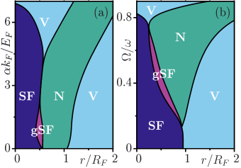
Figure 5: (Color online) Radial phase profiles are shown as a function of (a) $\alpha$ for $E_{b}=0.1E_{F}$ and $\Omega=0.4\omega$, and (b) $\Omega$ for $E_{b}=0.1E_{F}$ and $\alpha=0.4E_{F}/k_{F}$. The cooperation of $\Omega$ and $\alpha$ not only destroys the central SF core but also boosts the gSF region in both figures.

Next to Fig. 4(a), we present another phase diagram showing the destruction of the central SF core under more extreme parameter regimes. For instance, typical phase profiles for this case are illustrated in Fig. 5, where the interplay of fast $\Omega$ and/or large $\alpha$ eventually dominates the effects of $E_{b}\neq 0$ and depletes $n(0)$ to zero, recovering the non-interacting problem discussed above. The diagram shown in Fig. 4(b) is also one of our primary results in this paper, where $\Omega_{s}$ threshold for the complete destruction of the SF core is determined by first setting $\Delta\to 0$ as $r\to 0$ in Eq. (3) to get $\mu$, and then plugging these values to Eq. (4). This diagram intuitively suggests that $\Omega_{s}$ increases with increasing $E_{b}$ for a given $\alpha$. More importantly, it also shows that, in contrast to the $\alpha\to 0$ limit where the central SF pairs are robust against $\Omega<\omega$ for any $E_{b}$ since the centrifugal effects strictly vanish at $r=0$, increasing $\alpha$ eventually allows $\Omega$ to destroy all of the SF pairs.

V Conclusions

To summarize, here we studied the cooperation of adiabatic rotation and Rashba SOC on the ground-state phases of a trapped Fermi gas in two dimensions, assuming that vortices are not excited. First, by taking the harmonic confinement into account via both the LDA and exact approaches, we found the parameter regime where the non-interacting gas forms a ring-shaped annulus. It is important to emphasize that neither rotation nor SOC alone can deplete the central density to zero no matter how fast the rotation or large SOC is, and the formation of such an intriguing annulus requires them both simultaneously. Then, by taking the interactions into account via the BCS mean-field, we analyzed the rotation-induced pair-breaking mechanism in the entire BCS-BEC evolution. In particular, we showed that the cooperation of rotation and SOC allows for the possibility of creating either an isolated annulus of rigidly-rotating N particles that is disconnected from the central core of non-rotating SF pairs or an intermediate gapless SF phase which is charecterized by the coexistence of SF pairs and N particles. We also constructed phase diagrams showing the very first emergence of an N phase and the complete destruction of the central SF core. We hope that, given the ongoing push towards simulating Rashba-coupled Fermi gases by many groups worldwide, our compelling results may soon be realized once the technical experimental difficulties are cleared out of the way.

VI Acknowledgments

This work is supported by TÜB$\dot{\mathrm{I}}$TAK Grant No. 1001-114F232 and E. D. is supported by the TÜB$\dot{\mathrm{I}}$TAK-2215 Ph.D. Fellowship.

Appendix A Exact numerical solution for Sec. III

In the rotating frame, the non-interacting Hamiltonian for a harmonically-trapped Fermi gas with Rashba SOC can be written as

$$H_{0}=\int d\mathbf{r}\,\psi^{\dagger}(\mathbf{r})\left[H_{\mathrm{HO}}-\Omega L_{z}-\mu+\alpha\mathbf{p}\cdot\vec{\mathbf{\sigma}}\right]\psi(\mathbf{r})\,,$$ (7)

where $H_{\mathrm{HO}}=\mathbf{p}^{2}/(2M)+M\omega^{2}r^{2}/2$ is the usual two-dimensional harmonic-oscillator Hamiltonian. We make use of the rotational symmetry of the system, and expand the field operators in terms of the angular-momentum basis of the two-dimensional harmonic oscillator as

$$\psi_{\sigma}(\mathbf{r})=\sum_{n,l}g_{n,l}(\mathbf{r})c_{n,l,\sigma}\,,$$ (8)

where $c_{n,l,\sigma}$ annihilates a spin $\sigma$ particle in the $|n,l\rangle$ state that is given by the normalized real-space wave function

$$g_{n,l}(\mathbf{r})=i^{2n_{{}_{<}}}\sqrt{\frac{n_{{}_{<}}!}{\pi a_{0}^{2}n_{{}_{>}}!}}e^{il\theta}\tilde{r}^{|l|}e^{-\tilde{r}^{2}/2}L^{|l|}_{n_{{}_{<}}}\left(\tilde{r}^{2}\right)\;,$$ (9)

where $\tilde{r}=r/a_{0}$ with the harmonic-oscillator length $a_{0}=\sqrt{1/(M\omega)}$ scale, the energy and angular-momentum quantum numbers $n\geq|l|\geq 0$ are integers, $n_{{}_{<}}/n_{{}_{>}}$ is the lesser/greater of $(n\pm l)/2$, and $L^{|m|}_{k}(x)=(x^{-|m|}e^{x}/k!)d^{k}(e^{-x}x^{k+|m|})/dx^{k}.$ is the $k^{\mathrm{th}}$-degree associated Laguerre polynomial. The non-interacting Hamiltonian can be written in this basis as

$$H_{0} = \sum_{n,l,\sigma}\left[\omega(n+1)-\Omega l-\mu\right]c_{n,l,\sigma}^{\dagger}c_{n,l,\sigma}$$ (10)

$$+\frac{\alpha}{2a_{0}}\sum_{n,l}\left(i\sqrt{\frac{n+l}{2}+1}c_{n+1,l+1,\downarrow}^{\dagger}c_{n,l,\uparrow}\right.$$

$$\left.-i\sqrt{\frac{n-l}{2}}c_{n-1,l+1,\downarrow}^{\dagger}c_{n,l,\uparrow}+\textrm{H.c.}\right),$$

where H.c. is the Hermitian conjugate. Even though the Rashba coupling $\alpha\mathbf{p}\cdot\vec{\mathbf{\sigma}}$ does not preserve the individual spin or real-space rotational symmetry, the full rotational symmetry is still manifest. Since $H_{0}$ commutes with the total angular-momentum operator $J_{z}=L_{z}+S_{z}=\sum_{n,l,\sigma}\left(l+\frac{\sigma_{z}}{2}\right)c_{n,l,\sigma}^{\dagger}c_{n,l,\sigma},$ where $\sigma_{z}=\pm 1$ for $\sigma=(\uparrow,\downarrow)$, respectively, they can be simultaneously diagonalized.

Using the conservation of $J_{z}$, the Hamiltonian can be expressed in a block-diagonal form, $H_{0}=\sum_{l}\Psi^{\dagger}_{l}H_{l}\Psi_{l},$ where $H_{l}$ is a tri-diagonal matrix in each block with the following ordering of the basis states. For $l\geq 0$ corresponding to the $J_{z}$ subspace ($l\uparrow,l+1\downarrow$) with eigenvalue $j=l+1/2>0$, $H_{l}$ is given by

$$\begin{pmatrix}\epsilon_{l,l}&a\sqrt{l+1}&&&\\ a^{*}\sqrt{l+1}&\epsilon_{l+1,l+1}&a\sqrt{1}&&\\ &a^{*}\sqrt{1}&\epsilon_{l+2,l}&a\sqrt{l+2}&\\ &&a^{*}\sqrt{l+2}&\epsilon_{l+3,l+1}&a\sqrt{2}&\\ &&&a^{*}\sqrt{2}&\epsilon_{l+4,l}&\ddots\\ &&&&\ddots&\ddots\end{pmatrix},$$ (11)

where the basis vectors are ordered as $\Psi^{\dagger}_{l}=(c^{\dagger}_{n=l,l,\uparrow},c^{\dagger}_{l+1,l+1,\downarrow},c^{\dagger}_{l+2,l,\uparrow},c^{\dagger}_{l+3,l+1,\downarrow},\dots),$ Here, $\epsilon_{n,l}=\omega(n+1)-\Omega l-\mu$ and $a=i\alpha/2a_{0}$. Similarly for $l<0$ corresponding to the ($-|l|+1\downarrow,-|l|\uparrow$) subspace with eigenvalue $j=l+1/2<0$, $H_{l}$ is given by

$$\begin{pmatrix}\epsilon_{-l-1,l+1}&a\sqrt{-l}&&&\\ a^{*}\sqrt{-l}&\epsilon_{-l,l}&a\sqrt{1}&&\\ &a^{*}\sqrt{1}&\epsilon_{-l+1,l+1}&a\sqrt{-l+1}&\\ &&a^{*}\sqrt{-l+1}&\epsilon_{-l+2,l}&a\sqrt{2}&\\ &&&a^{*}\sqrt{2}&\epsilon_{-l+3,l+1}&\ddots\\ &&&&\ddots&\ddots\end{pmatrix},$$ (12)

where the basis vectors are ordered as $\Psi^{\dagger}_{l}=(c_{n=-l-1,l+1,\downarrow},c_{-l,l,\uparrow},c_{-l+1,l+1,\downarrow},c_{-l+2,l,\uparrow},\dots).$ This Hamiltonian can be diagonalized via the unitary transformation $c_{n,l,\sigma}=\sum_{m}u^{(j)}_{n\sigma,m}C_{j,m},$ leading to $H_{0}=\sum_{j,m}E^{(j)}_{m}C_{j,m}^{\dagger}C_{j,m},$ where $j=l+\sigma_{z}/2$ and the $\{u^{(j)}_{n\sigma,m}\}$ is the eigenvector characterizing the $m^{\textrm{th}}$ energy eigenstate in the $j=l+1/2$ subspace.

Note that this particular form of the Hamiltonian is similar to that of a Bogoliubov-de Gennes Hamiltonian of a harmonically-trapped spinless $p$-wave superconductor Stone2008 . Furthermore, the complex number $i$ in the complex factor $a$ can be absorbed in the even numbered eigenvector components so that numerically a tri-diagonal symmetric matrix can be diagonalized. In practice, a cut-off energy $E_{c}=\omega(l_{\mathrm{max}}+1)\gg E_{F}$ is introduced and finite matrices are diagonalized with basis states having less energy than the cut-off. We checked that our numerical results for the the low-energy eigenvalues and eigenvectors are independent of the chosen cut-off.

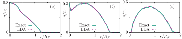
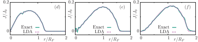
Figure 6: (Color online) Exact solutions for the (a)-(c) number density, and (d)-(f) mass-current density are compared with those of semi-classical LDA approach, where $\Omega/\omega=0.5$ in (a) and (d), $0.68$ in (b) and (e), and $0.7$ in (c) and (f). We also set $N=800$ and $\alpha=1.33E_{F}/k_{F}$ in all figures. The overall results are in excellent agreement with each other up to minor deviations due to finite-size effects.

Since SOC couples $\uparrow$ and $\downarrow$ spins, the mass-current density should be identified from the continuity equation

$$\partial_{t}\rho(\mathbf{r})+\mathbf{\nabla}\cdot\mathbf{J(\mathbf{r})}=0,$$ (13)

where $\rho(\mathbf{r})=Mn(\mathbf{r})$ is the mass density. The expectation value of the density and mass-current density operators are given as

$$n(r) = \sum_{\sigma}\langle\psi_{\sigma}^{\dagger}(r)\psi_{\sigma}(r)\rangle$$ (14)

$$= \sum_{n,n^{\prime},l,l^{\prime},\sigma}g^{*}_{n,l}(r)g_{n^{\prime},l^{\prime}}(r)\langle c_{n,l,\sigma}^{\dagger}c_{n^{\prime},l^{\prime},\sigma}\rangle$$

$$= \sum_{j}\sum_{m}\left[n^{(j)}_{\uparrow,m}(r)+n^{(j)}_{\downarrow,m}(r)\right]f\left[E_{m}^{(j)}\right],$$

$$J_{\theta}(r) = \sum_{\sigma}\Im\langle\psi_{\sigma}^{\dagger}(r)\frac{\partial}{r\partial\theta}\psi_{\sigma}(r)\rangle+2M\alpha|\langle\psi_{\uparrow}^{\dagger}(r)\psi_{\downarrow}(r)\rangle|$$ (15)

$$= M\sum_{j}\sum_{m}J_{\theta,m}^{(j)}(r)f\left[E_{m}^{(j)}\right],$$

where $f\left[E_{m}^{(j)}\right]=\langle C_{j,m}^{\dagger}C_{j,m}\rangle$ with $\langle\cdots\rangle$ the thermal average and $f(x)=1/(e^{\beta x}+1)$ is the Fermi-Dirac distribution, and $\Im$ denotes imaginary part. Here, the density $n^{(j)}_{\sigma,m}(r)$ and the angular component of the mass current density $J_{\theta,m}^{(j)}(r)$ for the $m^{\textrm{th}}$ energy eigenstate with total angular momentum $j$ are given by

$$n^{(j)}_{\uparrow,m}(r) =\left\lvert\sum_{k=0}^{n_{c}/2}u^{(j)}_{l+2k\uparrow,m}g_{l+2k,l}(r,\theta)\right\rvert^{2},$$ (16)

$$n^{(j)}_{\downarrow,m}(r) =\left\lvert\sum_{k=0}^{n_{c}/2}u^{(j)}_{l+1+2k\downarrow,m}g_{l+2k,l+1}(r,\theta)\right\rvert^{2},$$ (17)

$$J_{\theta,m}^{(j)}(r) =\frac{l}{r}n^{(j)}_{\uparrow,m}(r)+\frac{l+1}{r}n^{(j)}_{\downarrow,m}(r)$$ (18)

$$+2\alpha\left\lvert\left[\sum_{k=0}^{n_{c}/2}u^{(j)}_{l+2k\uparrow,m}g_{l+2k,l}(r,\theta)\right]^{*}\right.$$ (19)

$$\left.\left[\sum_{k=0}^{n_{c}/2}u^{(j)}_{l+1+2k\downarrow,m}g_{l+2k,l+1}(r,\theta)\right]\right\rvert,$$ (20)

for $j>0$ ($l\geq 0$) and

$$n^{(j)}_{\uparrow,m}(r) =\left\lvert\sum_{k=0}^{n_{c}/2}u^{(j)}_{-l+2k\uparrow,m}g_{l+2k,l}(r,\theta)\right\rvert^{2},$$ (21)

$$n^{(j)}_{\downarrow,m}(r) =\left\lvert\sum_{k=0}^{n_{c}/2}u^{(j)}_{-l-1+2k\downarrow,m}g_{l+2k,l+1}(r,\theta)\right\rvert^{2},$$ (22)

$$J_{\theta,m}^{(j)}(r) =\frac{l}{r}n^{(j)}_{\uparrow,m}(r)+\frac{l+1}{r}n^{(j)}_{\downarrow,m}(r)$$ (23)

$$+2\alpha\left\lvert\left[\sum_{k=0}^{n_{c}/2}u^{(j)}_{-l+2k\uparrow,m}g_{l+2k,l}(r,\theta)\right]^{*}\right.$$ (24)

$$\left.\left[\sum_{k=0}^{n_{c}/2}u^{(j)}_{-l-1+2k\downarrow,m}g_{l+2k,l+1}(r,\theta)\right]\right\rvert,$$ (25)

for $j<0$ ($l<0$) and $n_{c}=(|l|_{\mathrm{max}}-|l|)/2$. The density is independent of the angle $\theta$ and the radial component of the mass-current density is zero for the energy eigenstates.

In Fig. 6, we present the number and mass-current density profiles in the trap that are obtained from the exact calculation given above and the LDA approach described in the main text, showing an excellent agreement between the two. The total number of particles is $N=2\pi\int\textrm{d}r\,rn(r)=800$. The finite-size effects vanish in the thermodynamic limit when $N\to\infty$.

In comparing the exact quantum-mechanical calculations with LDA, we scale the radial distance by the Thomas-Fermi radius $R_{F}$ and the density by $n_{0}=k_{F}^{2}/(2\pi)$, which are defined via $E_{F}=k_{F}^{2}/(2M)=M\omega^{2}R_{F}/2$. Here, the Fermi energy is defined for the non-rotating gas in the absence of an SOC as $E_{F}=\omega\sqrt{N}$ in LDA, so that $(k_{F}a_{0})^{2}=2\sqrt{N}$ and $R_{F}/a_{0}=(4N)^{1/4}$. In this case, the exact quantum-mechanical solution gives $E_{F}=\omega(N_{F}+1)$ and $N=(N_{F}+1)(N_{F}+2)$ with the quantum number $N_{F}$. This is consistent with the LDA result $E_{F}=\omega\sqrt{N}$ for large number of particles $N$ in the trap such that $N_{F}\gg 1$. The mass-current density is in units of $J_{0}=Mn_{0}\omega R_{F}=\sqrt{2}N^{3/4}/(\pi a_{0}^{3})$.

References

- (1) J. R. Abo-Shaeer, C. Raman, J. M. Vogels, and W. Ketterle, Science 292, 476 (2001).
- (2) M.W. Zwierlein and J.R. Abo-Shaeer, A. Schirotzek, C.H.Schunck, W. Ketterle, Nature 435, 1047 (2005).
- (3) T.L. Ho and C.V. Ciobanu, Phys. Rev. Lett. 85, 4648 (2000).
- (4) N. R. Cooper, N. K. Wilkin, and J. M. F. Gunn, Phys. Rev. Lett. 87, 120405 (2001).
- (5) U.R. Fischer and G. Baym, Phys. Rev. Lett. 90, 140402 (2003).
- (6) M. A. Baranov, K. Osterloh, and M. Lewenstein, Phys. Rev. Lett. 94, 070404 (2005).
- (7) M. Z. Hasan and C. L. Kane, Rev. Mod. Phys. 82, 3045 (2010).
- (8) X.-L. Qi and S.-C. Zhang, Rev. Mod. Phys. 83, 1057 (2011).
- (9) J. Sinova, S. O. Valenzuela, J. Wunderlich, C. H. Back, and T. Jungwirth, to appear in Rev. Mod. Phys. (2015).
- (10) I. Žutić and S. Das Sarma, Rev. Mod. Phys. 76, 323 (2004).
- (11) Y.-J. Lin, Jiménez-García, and I. B. Spielman, Nature 471, 83 (2011).
- (12) J. Y. Zhang, S. C. Ji, Z. Chen, L. Zhang, Z. D. Du, Bo Yan, G. S. Pan, B. Zhao, Y. J. Deng, H. Zhai, S. Chen, and J. W. Pan, Phys. Rev. Lett. 109, 115301 (2012).
- (13) P. Wang, Z.-Q. Yu, Z. Fu, J. Miao, L. Huang, S. Chai, H. Zhai, and J. Zhang, Phys. Rev. Lett. 109, 095301 (2012).
- (14) L.W. Cheuk, A.T. Sommer, Z. Hadzibabic, T. Yefsah, W.S. Bakr, and M.W. Zwierlein, Phys. Rev. Lett. 109,095302 (2012).
- (15) C. Qu, C. Hamner, M. Gong, C. Zhang, and P. Engels, Phys. Rev. A 88, 021604(R) (2013).
- (16) A. J. Olson, S.-J. Wang, R. J. Niffenegger, C.-H. Li, C. H. Greene, and Y. P. Chen, Phys. Rev. A 90, 013616 (2014).
- (17) N. Goldman, G. Juzelinas, P. Öhberg, and I. B. Spielman, Rep. Prog. Phys. 77, 126401 (2014).
- (18) K. Jiménez-García, L. LeBlanc, R.Williams, M. Beeler, C. Qu, M. Gong, C. Zhang, and I. Spielman, Phys. Rev. Lett. 114, 125301 (2015).
- (19) L. Huang, Z. Meng, P. Wang, P. Peng, S.-L. Zhang, L. Chen, D. Li, Q. Zhou, and Jing Zhang, arXiv:1506.02861 (2015).
- (20) J. Ruseckas, G. Juzelinas, P. Öhberg, and M. Fleischhauer, Phys. Rev. Lett. 95, 010404 (2005).
- (21) D. L. Campbell, G. Juzelinas, and I. B. Spielman, Phys. Rev. A 84, 025602 (2011).
- (22) Z. F. Xu and L. You, Phys. Rev. A 85, 043605 (2012).
- (23) J.P. Vyasanakere, S. Zhang, and V.B. Shenoy, Phys. Rev. B 84, 014512 (2011).
- (24) Z.-Q. Yu and H. Zhai, Phys. Rev. Lett. 107, 195305 (2011).
- (25) M. Iskin and A. L. Subaşı, Phys. Rev. Lett. 107, 050402 (2011).
- (26) M. Gong, S. Tewari, and C. Zhang, Phys. Rev. Lett. 107, 195303 (2011).
- (27) W. Yi and G.-C. Guo, Phys. Rev. A 84, 031608(R) (2011).
- (28) L. Jiang, X.-J. Liu, H. Hu, and H. Pu, Phys. Rev. A 84, 063618 (2011).
- (29) K. Zhou and Z. Zhang, Phys. Rev. Lett. 108, 025301 (2012).
- (30) R. Liao, Y. Y.-Xiang, and W.-M. Liu, Phys. Rev. Lett. 108, 080406 (2012).
- (31) K. Seo, Li Han and C. A. R. Sá de Melo, Phys. Rev. Lett. 109, 105303 (2012).
- (32) S. Takei, C.-H. Lin, B. M. Anderson, and V. Galitski, Phys. Rev. A 85, 023626 (2012).
- (33) L. He and X.-G. Huang, Phys. Rev. Lett. 108, 145302 (2012).
- (34) M. Gong, G. Chen, S. Jia, and C. Zhang, Phys. Rev. Lett. 109, 105302 (2012).
- (35) A. Ambrosetti, G. Lombardi, L. Salasnich, P. L. Silvestrelli, and F. Toigo, Phys. Rev. A 90, 043614 (2014).
- (36) X. Yang and S. Wan, Phys. Rev. A 85, 023633 (2012).
- (37) W. Zhang and W. Yi, Nat. Commun. 4, 2711 (2013).
- (38) M. Iskin, Phys. Rev. A 88, 013631 (2013).
- (39) Ye Cao, Shu-Hao Zou, Xia-Ji Liu, Su Yi, Gui-Lu Long, and Hui Hu, Phys. Rev. Lett. 113, 115302 (2014).
- (40) K. Martiyanov, V. Makhalov, and A. Turlapov, Phys. Rev. Lett. 105, 030404 (2010).
- (41) P. Dyke, E. D. Kuhnle, S. Whitlock, H. Hu, M. Mark, S. Hoinka, M. Lingham, P. Hannaford, and C. J. Vale, Phys. Rev. Lett. 106, 105304 (2011).
- (42) B. Fröhlich, M. Feld, E. Vogt, M. Koschorreck, W. Zwerger, and M. Köhl, Phys. Rev. Lett. 106, 105301 (2011).
- (43) M. Feld, B. Fröhlich, E. Vogt, M. Koschorreck, and M. Köhl, Nature 480, 75 (2011).
- (44) A. T. Sommer, L. W. Cheuk, M. J. H. Ku, W. S. Bakr, and M. W. Zwierlein, Phys. Rev. Lett. 108, 045302 (2012).
- (45) M. G. Ries, A. N. Wenz, G. Zrn, L. Bayha, I. Boettcher, D. Kedar, P. A. Murthy, M. Neidig, T. Lompe, and S. Jochim, Phys. Rev. Lett. 114, 230401 (2015).
- (46) I. Bausmerth, A. Recati, and S. Stringari, Phys. Rev. Lett. 100, 070401 (2008).
- (47) I. Bausmerth, A. Recati, and S. Stringari, Phys. Rev. A 78, 063603 (2008).
- (48) M. Urban and P. Schuck, Phys. Rev. A 78, 011601 (2008).
- (49) M. Iskin and E. Tiesinga, Phys. Rev. A 79, 053621 (2009).
- (50) H. J. Warringa and A. Sedrakian, Phys. Rev. A 84, 023609 (2011).
- (51) H. J. Warringa, Phys. Rev. A 86, 043615 (2012).
- (52) J. Radić, T. A. Sedrakyan, I. B. Spielman, and V. Galitski, Phys. Rev. A 84, 063604 (2011).
- (53) M. Stone and I. Anduaga, Ann. Phys. (N. Y). 323, 2 (2008).