New upper bounds for the density of translative packings of three-dimensional convex bodies with tetrahedral symmetry

Abstract.

In this paper we determine new upper bounds for the maximal density of translative packings of superballs in three dimensions (unit balls for the $l^{p}_{3}$-norm) and of Platonic and Archimedean solids having tetrahedral symmetry. Thereby, we improve Zong’s recent upper bound for the maximal density of translative packings of regular tetrahedra from $0.3840\ldots$ to $0.3745\ldots$, getting closer to the best known lower bound of $0.3673\ldots$

We apply the linear programming bound of Cohn and Elkies which originally was designed for the classical problem of densest packings of round spheres. The proofs of our new upper bounds are computational and rigorous. Our main technical contribution is the use of invariant theory of pseudo-reflection groups in polynomial optimization.

1. Introduction

The most famous geometric packing problem is Kepler’s conjecture from 1611: The density of any packing of equal-sized spheres into three-dimensional Euclidean space is never greater than $\pi/\sqrt{18}=0.7404\ldots$ This density is achieved for example by the “cannonball” packing. In 1998 Hales and Ferguson solved Kepler’s conjecture. Their proof is extremely complicated, involving more than 200 pages, intensive computer calculations, and checking of more than 5,000 subproblems. They wrote a book [25] that contains the entire proof together with supporting material and commentary.

Very little is known if one goes beyond three-dimensional packings of spheres to packings of nonspherical objects. Considering nonspherical objects is interesting for many reasons. For example, using nonspherical objects one can model physical granular materials accurately. On the other hand, the mathematical difficulty increases substantially when one deals with nonspherical objects.

Jiao, Stillinger, and Torquato [29] consider packings of three-dimensional superballs, which are unit balls of the $l^{p}_{3}$-norm, with $p\geq 1$:

$$B^{p}_{3}=\{(x_{1},x_{2},x_{3})\in\mathbb{R}^{3}:|x_{1}|^{p}+|x_{2}|^{p}+|x_{3}|^{p}\leq 1\}.$$

Three-dimensional superballs can be synthesized experimentally as colloids, see Rossi et al. [41]. The name “superball” is attributed to the Danish inventor Piet Hein who used a “superellipse” with $p=5/2$ in a design challenge of the redevelopment of the public square Sergels Torg in Stockholm (see also Rush and Sloane [42], and Gardner [18]). Life Magazine [26] quotes Piet Hein:

Man is the animal that draws lines which he himself then stumbles over. In the whole pattern of civilization there have been two tendencies, one toward straight lines and rectangular patterns and one toward circular lines. There are reasons, mechanical and psychological, for both tendencies. Things made with straight lines fit well together and save space. And we can move easily—physically or mentally—around things made with round lines. But we are in a straitjacket, having to accept one or the other, when often some intermediate form would be better.

Back to the work of Jiao, Stillinger, and Torquato [29]. They construct the densest known packings of $B^{p}_{3}$ for many values of $p$. As motivation for their study Jiao, Stillinger, and Torquato write:

Understanding the organizing principles that lead to the densest packings of nonspherical particles that do not tile space is of great practical and fundamental interest. Clearly, the effect of asphericity is an important feature to include on the way to characterizing more fully real dense granular media.

[…]

On the theoretical side, no results exist that rigorously prove the densest packings of other congruent non-space-tiling particles in three dimension.

Torquato and Jiao [49, 50] extend the work on superballs to nonspherical non-differentiable shapes. They found dense packings of Platonic and of Archimedean solids.

Very little is known about the densest packings of polyhedral particles that do not tile space, including the majority of the Platonic and Archimedean solids studied by the ancient Greeks. The difficulty in obtaining dense packings of polyhedra is related to their complex rotational degrees of freedom and to the non-smooth nature of their shapes.

The optimal, densest lattice packing of each Platonic or Archimedean solid is known. Minkowski [35] determines the densest lattice packing of regular octahedra. Hoylman [27] uses Minkowski’s method to determine the densest lattice packing of regular tetrahedra. Betke and Henk [3] turn Minkowski’s method into an implementable algorithm and find the densest lattice packings of all remaining Platonic and all Archimedean solids. Only two of the Platonic and Archimedean solids are not centrally symmetric, namely the tetrahedron and the truncated tetrahedron. These are also the only cases where Torquato and Jiao could use the extra freedom of rotating the solids to find new packings which are denser than the corresponding densest lattice packings. Also the dense superball packings of Jiao, Stillinger, and Torquato are lattice packings. Based on this evidence they formulate the following conjecture:

The densest packings of the centrally symmetric Platonic and Archimedean solids are given by their corresponding optimal lattice packings. This is the analogue of Kepler’s sphere conjecture for these solids.

For a convex body $\mathcal{K}$ in $\mathbb{R}^{n}$ it is natural to consider three kinds of increasingly restrictive packings: congruent packings, translative packings, and lattice packings. A packing of congruent copies of $\mathcal{K}$ has the form

$$\mathcal{P}=\bigcup_{i\in\mathbb{N}}(x_{i}+A_{i}\mathcal{K}),\quad\text{with }(x_{i},A_{i})\in\mathbb{R}^{n}\times\mathrm{SO}(n),\;i\in\mathbb{N},$$

where $x_{i}+A_{i}\mathcal{K}^{\circ}\cap x_{j}+A_{j}\mathcal{K}^{\circ}=\emptyset$ whenever the indices $i$ and $j$ are distinct. Here, $\mathcal{K}^{\circ}$ denotes the topological interior of the body $\mathcal{K}$ and

$$\mathrm{SO}(n)=\{A\in\mathbb{R}^{n\times n}:AA^{\sf T}=I_{n},\,\det A=1\}$$

denotes the special orthogonal group, an index-$2$ subgroup of the orthogonal group

$$\mathrm{O}(n)=\{A\in\mathbb{R}^{n\times n}:AA^{\sf T}=I_{n}\}.$$

The (upper) density of $\mathcal{P}$ is

$$\delta(\mathcal{P})=\limsup_{r\to\infty}\sup_{c\in\mathbb{R}^{n}}\frac{\operatorname{vol}(B(c,r)\cap\mathcal{P})}{\operatorname{vol}B(c,r)},$$

where $B(c,r)$ is the Euclidean ball of radius $r$ centered at $c$. A packing $\mathcal{P}$ is called a translative packing if each rotation $A_{i}$ is identity. A translative packing is called a lattice packing if the set of $x_{i}$’s forms a lattice.

Lattice packings are restrictive and many results about them are known. This is not the case for translative and congruent packings. While the conjecture of Torquato and Jiao ultimately aims at congruent packings, the objective of our paper is to develop tools coming from mathematical optimization which will be useful to make progress on the conjecture restricted to translative packings. In particular we prove new upper bounds for the density of densest translative packings of three-dimensional superballs and of Platonic and Archimedean solids with tetrahedral symmetry. We use the following theorem of Cohn and Elkies [6] for this.

Theorem 1.1.

Let $\mathcal{K}$ be a convex body in $\mathbb{R}^{n}$ and let $f\colon\mathbb{R}^{n}\to\mathbb{R}$ be a continuous $L^{1}$-function (a continuous function whose absolute value is Lebesgue integrable). Define the Fourier transform of $f$ at $u$ by

$$\widehat{f}(u)=\int_{\mathbb{R}^{n}}f(x)e^{-2\pi iu\cdot x}\,dx.$$

Suppose $f$ satisfies the following conditions

1. $\widehat{f}(0)\geq 1$,

2. $f$ is of positive type, i.e. $\widehat{f}(u)\geq 0$ for every $u\in\mathbb{R}^{n}$,

3. $f(x)\leq 0$ whenever $\mathcal{K}^{\circ}\cap(x+\mathcal{K}^{\circ})=\emptyset$.

Then the density of any packing of translates of $\mathcal{K}$ in $\mathbb{R}^{n}$ is at most $f(0)\operatorname{vol}\mathcal{K}$.

One can find a proof of this theorem in Cohn and Kumar [7] or for the more general case of translative packings of multiple convex bodies $\mathcal{K}_{1},\ldots,\mathcal{K}_{N}$ in de Laat, Oliveira, and Vallentin [33]. Originally, Cohn and Elkies [6] state the theorem only for admissible functions; these are functions for which the Poisson summation formula applies.

The Cohn-Elkies bound provides the basic framework for proving the best known upper bounds for the maximum density of sphere packings in dimensions $4$, …, $36$. For some time it was conjectured to provide tight bounds in dimensions $8$ and $24$ and there was very strong numerical evidence to support this conjecture, see Cohn and Miller [9]. However, the only thing missing was a rigorous proof. Recently, in March 2016, such a proof was found by Viazovska [51] for dimension $8$ and a few days later, building on Viazovska’s breakthrough result, by Cohn, Kumar, Miller, Radchenko, and Viazovska [8] for dimension $24$. Here the explicit construction of optimal functions $f$ uses the theory of quasimodular forms from analytic number theory.

De Laat, Oliveira, and Vallentin [33] have proposed a strengthening of the Cohn-Elkies bound and computed better upper bounds for the maximum density of sphere packings in dimensions $4$, $5$, $6$, $7$, and $9$.

In all these calculations one can restrict the function $f$ to be a radial function (a function whose values $f(x)$ only depend on the norm $\|x\|$ of the vector $x\in\mathbb{R}^{n}$) because of the rotational symmetry of the sphere. For the case of packings of nonspherical objects Cohn and Elkies [6] write:

Unfortunately, when [the body we want to pack] is not a sphere, there does not seem to be a good analogue of the reduction to radial functions in Theorem [1.1]. That makes these cases somewhat less convenient to deal with.

Until now, the Cohn-Elkies bound has only been computed for packings of spheres. In this paper we show how to apply the Cohn-Elkies bound for nonspherical objects.

1.1. New upper bounds for translative packings

Before we describe our methods we report on the new upper bounds we obtained and compare them to the known lower and upper bounds. We give the new upper bounds for three-dimensional superball packings in Table 1, the new upper bounds for Platonic and Archimedean solid with tetrahedral symmetry are in Table 2.

Body	Lattice packing
	lower bound	upper bound
$B_{3}^{1}$	$18/19=0.9473\dots$ [35]	$18/19$ [35]
$B_{3}^{2}$	$\pi/\sqrt{18}=0.7404\dots$	$\pi/\sqrt{18}$ [20]
$B_{3}^{3}$	$0.8095\dots$ [29]	$\mathit{0.8236\dots}$
$B_{3}^{4}$	$0.8698\dots$[29]	$\mathit{0.8742\dots}$
$B_{3}^{5}$	$0.9080\dots$ [29]	$\mathit{0.9224\dots}$
$B_{3}^{6}$	$0.9318\dots$ [29]	$\mathit{0.9338\dots}$

	Translative packing
	lower bound	upper bound
$B_{3}^{1}$	$18/19=0.9473\dots$ [35]	$\mathit{0.9729\dots}$
$B_{2}^{2}$	$\pi/\sqrt{18}=0.7404\dots$	$\pi/\sqrt{18}$ [25]
$B_{3}^{3}$	$0.8095\dots$ [29]	$\mathit{0.8236\dots}$
$B_{3}^{4}$	$0.8698\dots$ [29]	$\mathit{0.8742\dots}$
$B_{3}^{5}$	$0.9080\dots$ [29]	$\mathit{0.9224\dots}$
$B_{3}^{6}$	$0.9318\dots$ [29]	$\mathit{0.9338\dots}$

	Congruent packing
	lower bound	upper bound
$B_{3}^{1}$	$18/19=0.9473\dots$ [35]	$1-1.4\ldots\cdot 10^{-12}$ [23]
$B_{2}^{2}$	$\pi/\sqrt{18}=0.7404\dots$	$\pi/\sqrt{18}$ [25]
$B_{3}^{3}$	$0.8095\dots$ [29]	$<1$
$B_{3}^{4}$	$0.8698\dots$ [29]	$<1$
$B_{3}^{5}$	$0.9080\dots$ [29]	$<1$
$B_{3}^{6}$	$0.9318\dots$ [29]	$<1$

Table 1. Best known bounds for packings of three-dimensional superballs. New bounds obtained in this paper are written in italics.

Body	Lattice packing
	lower bound	upper bound
Tetrahedron	$18/49=0.3673\dots$ [24]	$18/49$ [27]
Truncated tetrahedron	$0.6809\dots$ [3]	$0.6809\dots$ [3]
Truncated cuboctahedron	$0.8493\dots$ [3]	$0.8493\dots$ [3]
Rhombicuboctahedron	$0.8758\dots$ [3]	$0.8758\dots$ [3]
Cuboctahedron	$0.9183\dots$ [24]	$0.9183\dots$ [27]
Truncated cube	$0.9737\dots$ [3]	$0.9737\dots$ [3]

	Translative packing
	lower bound	upper bound
Tetrahedron	$18/49=0.3673\dots$ [24]	$\mathit{0.3745\dots}$
Truncated tetrahedron	$0.6809\dots$ [3]	$\mathit{0.7292\dots}$
Truncated cuboctahedron	$0.8493\dots$ [3]	$0.8758\dots$ [50]
Rhombicuboctahedron	$0.8758\dots$ [3]	$0.8758\dots$ [22]
Cuboctahedron	$0.9183\dots$ [24]	$\mathit{0.9364\dots}$
Truncated cube	$0.9737\dots$ [3]	$\mathit{0.9845\dots}$

	Congruent packing
	lower bound	upper bound
Tetrahedron	$4000/4671=0.8563\dots$ [5]	$1-2.6\ldots\cdot 10^{-25}$ [23]
Truncated tetrahedron	$207/208=0.9951\dots$ [31], [11]	$<1$
Truncated cuboctahedron	$0.8493\dots$ [3]	$0.8758\dots$ [50]
Rhombicuboctahedron	$0.8758\dots$ [3]	$0.8758\dots$ [22]
Cuboctahedron	$0.9183\dots$ [24]	$<1$
Truncated cube	$0.9737\dots$ [3]	$<1$

Table 2. Best known bounds for packings of three-dimensional Platonic and Archimedean solids with tetrahedral symmetry. The octahedron, the cube and the truncated octahedron are omitted. New bounds obtained in this paper are written in italics.

1.1.1. Three-dimensional superballs

Jiao, Stillinger, and Torquato [29, 30] find dense packings of superballs $B^{p}_{3}$ for all values of $p\geq 1$. Although they principally allow congruent packings in their computer simulations, the dense packings they find are all lattice packings. They subdivide the range $p\in[1,\infty)$ into four different regimes

$$p\in[1,2\ln 3/\ln 4=1.5849\ldots]\cup[1.5849\ldots,2]\cup[2,2.3018\ldots]\cup[2.3018\ldots,\infty)$$

and give for each regime a family of lattices determining dense packings. When $p=1$ then $B^{p}_{3}$ is simply the regular octahedron, a Platonic solid. The optimal lattice packing of regular octahedra has been determined by Minkowski [35].

Recently, Ni, Gantapara, de Graaf, van Roij, and Dijkstra [36] claimed that for values of $p$ lying in the interior of the first and respectively of the second regime, the packings of Jiao, Stillinger, and Torquato can be improved.

When $p=2$, then $B^{p}_{3}$ is the round unit ball of Euclidean space. The optimal lattice packing of $B^{2}_{3}$ has been determined by Gauss [20] using reduction theory of positive quadratic forms. Here, translative and congruent packings coincide because of the rotational symmetry of $B^{2}_{3}$. Hales [25] proved the optimality of the cannonball packing among all congruent packings. One should note that there is an uncountable family of non-lattice packings achieving the same density. The best upper bound obtainable from Theorem 1.1 is $0.7797\dots$

For $p\geq 2.3018\ldots$ the densest known superball packings are given by the family of $C_{1}$-lattices which is defined by $\mathbb{Z}b_{1}+\mathbb{Z}b_{2}+\mathbb{Z}b_{3}$ with

$$b_{1}=(2^{1-\frac{1}{p}},2^{1-\frac{1}{p}},0),\;b_{2}=(2^{1-\frac{1}{p}},0,2^{1-\frac{1}{p}}),\;b_{3}=(2s+2^{1-\frac{1}{p}},-2s,-2s),$$

where $s$ is the smallest positive root of the equation

$$(s+2^{-\frac{1}{p}})^{p}+2s^{p}-1=0,$$

having density

$$\frac{\operatorname{vol}B^{p}_{3}}{2^{3-\frac{2}{p}}(3s+2^{-\frac{1}{p}})}.$$

1.1.2. Platonic and Archimedean solids with tetrahedral symmetry

We prove a new upper bound for the density of densest translative packings of regular tetrahedra and improve the upper bound of $0.3840\ldots$ recently obtained by Zong [53] to $0.3745\ldots$ Groemer [24] shows that there is a lattice packing of regular tetrahedra which has density $0.3673\ldots$ and Hoylman [27] proves the optimality of Groemer’s packing among lattice packings using Minkowski’s method. Finding dense congruent packings of regular tetrahedra is fascinating. In fact, it is part of Hilbert’s 18th problem. We refer to Lagarias and Zong [34] for the history of the tetrahedra packing problem and to Ziegler [52] for an overview on a race for the best construction.

As a corollary of our new bound for the tetrahedron, we improve Zong’s bound for densest translative packings of the cuboctahedron from $0.9601\ldots$ to $0.9364\ldots$ This follows from Minkowski’s observation that

$$\bigcup_{i\in\mathbb{N}}(x_{i}+\mathcal{K})$$

is a translative packing of $\mathcal{K}$ if and only if

$$\bigcup_{i\in\mathbb{N}}\left(x_{i}+\frac{1}{2}(\mathcal{K}-\mathcal{K})\right)$$

is a packing of $\frac{1}{2}(\mathcal{K}-\mathcal{K})$, with

$$\mathcal{K}-\mathcal{K}=\{x-y:x,y\in\mathcal{K}\}$$

denoting the Minkowski difference of the body $\mathcal{K}$ with itself. The Minkowski difference of a regular tetrahedron with itself is the cuboctahedron whose volume is $2^{3}\cdot 5/2$ times the volume of the regular tetrahedron.

We omitted the octahedron from Table 2 because it is $B^{1}_{3}$ in Table 1. We also omitted the cube and the truncated octahedron because with both solids one can tile three-dimensional space.

1.2. Computational strategy

In this section we give a high level description of how we found suitable functions $f$ for Theorem 1.1 for proving the new upper bounds.

The symmetry group of a convex body $\mathcal{K}\subseteq\mathbb{R}^{n}$ is

$$S(\mathcal{K})=\{A\in\operatorname{O}(n):A\mathcal{K}=\mathcal{K}\},$$

and when considering functions $f$ for Theorem 1.1 the symmetry group of the Minkowski difference $\mathcal{K}-\mathcal{K}$ will be useful. For $A\in S(\mathcal{K}-\mathcal{K})$ we have

$$\begin{split}&A^{-1}x+\mathcal{K}^{\circ}\cap\mathcal{K}^{\circ}=\emptyset\Longleftrightarrow x+A\mathcal{K}^{\circ}\cap A\mathcal{K}^{\circ}=\emptyset\Longleftrightarrow x\not\in A\mathcal{K}^{\circ}-A\mathcal{K}^{\circ}\\ &\quad\Longleftrightarrow x\not\in A(\mathcal{K}^{\circ}-\mathcal{K}^{\circ})\Longleftrightarrow x\not\in\mathcal{K}^{\circ}-\mathcal{K}^{\circ}\Longleftrightarrow x+\mathcal{K}^{\circ}\cap\mathcal{K}^{\circ}=\emptyset.\end{split}$$

Hence we may assume without loss of generality that the function $f$ we are seeking is invariant under the left action of $S(\mathcal{K}-\mathcal{K})$, i.e.

$$f(A^{-1}x)=f(x)\quad\text{for all }A\in S(\mathcal{K}-\mathcal{K}).$$

This assumption reduces the search space and also makes the third constraint $f(x)\leq 0$ whenever $x+\mathcal{K}^{\circ}\cap\mathcal{K}^{\circ}=\emptyset$ easier to model.

In the case of $\mathcal{K}$ being a superball $B^{p}_{3}$, with $p\geq 1$ and $p\neq 2$, the Minkowski difference $\mathcal{K}-\mathcal{K}$ is $2B^{p}_{3}$ and its symmetry group is a finite subgroup of the orthogonal group. It is the octahedral group (which is the same as the symmetry group of the regular cube $[-1,+1]^{3}$), which has $48$ elements. The octahedral group is the reflection group $\mathsf{B}_{3}$ which is generated by the three matrices

(1) $$\begin{pmatrix}-1&0&0\\ 0&1&0\\ 0&0&1\end{pmatrix},\;\begin{pmatrix}1&0&0\\ 0&0&-1\\ 0&-1&0\end{pmatrix},\;\begin{pmatrix}0&0&1\\ 0&1&0\\ 1&0&0\end{pmatrix},$$

where the first one is the reflection at the plane $x_{1}=0$, the second one is the reflection at the plane $x_{2}+x_{3}=0$, and the last one is the reflection at the plane $x_{1}-x_{3}=0$.

In the case of $\mathcal{K}$ being a Platonic or Archimedean solid with tetrahedral symmetry, the symmetry group of the Minkowski difference $\mathcal{K}-\mathcal{K}$ is the octahedral group, too.

We specify the function $f\colon\mathbb{R}^{3}\to\mathbb{R}$ via its Fourier transform $\widehat{f}$. If $f$ is invariant under the action of $S(\mathcal{K}-\mathcal{K})$ then the same is true for its Fourier transform $\widehat{f}$. Let $g$ be a polynomial. We use the following template for the Fourier transform of $f$:

(2) $$\widehat{f}(u)=g(u)e^{-\pi\|u\|^{2}}.$$

So $\widehat{f}$ is a Schwartz function (i.e. all derivates $D^{\beta}\widehat{f}(x)$ exist for all $x\in\mathbb{R}^{n}$ and all $\beta\in\mathbb{N}^{n}$ and $\sup\{|x^{\alpha}D^{\beta}\widehat{f}(x)|:x\in\mathbb{R}^{n}\}<\infty$ holds for all $\alpha,\beta\in\mathbb{N}^{n}$), implying that also $f$ is a Schwartz function. In particular, $f$ will be a continuous $L^{1}$-function.

If $f$ is invariant under $\mathsf{B}_{3}$ then so is the polynomial $g$ which specifies $\widehat{f}$. This means that $g$ lies in the ring of invariants of the group $\mathsf{B}_{3}$ which is, by the theory of finite reflection groups, known to be freely generated by three basic invariants

(3) $$\theta_{1}=x_{1}^{2}+x_{2}^{2}+x_{3}^{2},\;\;\theta_{2}=x_{1}^{4}+x_{2}^{4}+x_{3}^{4},\;\;\theta_{3}=x_{1}^{6}+x_{2}^{6}+x_{3}^{6}.$$

Thus, we can assume that $g$ lies in the polynomial ring $\mathbb{R}[\theta_{1},\theta_{2},\theta_{3}]$.

The first condition of Theorem 1.1 is a simple linear condition in the coefficients of the polynomial $g$, it says

$$g(0)\geq 1.$$

For the second condition we want the function $f$ whose Fourier transform is given by (2) to be of positive type. This is true if and only if $g$ is globally nonnegative. In general, checking that a polynomial is nonnegative everywhere is computationally difficult, it is an NP-hard problem. We use a standard relaxation of the global nonnegativity constraint by imposing a sufficient condition which is easier to check: We want that $g$ can be written as a sum of squares, which we can formulate as a semidefinite condition. Furthermore, we can use the imposed $\mathsf{B}_{3}$-invariance of $g$ to simplify this semidefinite condition. In Section 2 we work out the theory of this simplification for the case of pseudo-reflection groups. In Section 3 we apply the theory to the finite reflection group $\mathsf{B}_{3}$.

Although using this sum of squares relaxation works very well in practice, we are indeed restricting the search space of functions. Hilbert showed in 1888 that there are polynomials already in two variables which are globally nonnegative but which are not sum of squares. Hilbert’s proof was nonconstructive and only in 1967 Motzkin published the first explicit example. Shortly afterwards Robinson showed that the $\mathsf{B}_{3}$-invariant polynomial

(4) $$x_{1}^{6}+x_{2}^{6}+x_{3}^{6}-(x_{1}^{4}x_{2}^{2}+x_{1}^{2}x_{2}^{4}+x_{1}^{4}x_{3}^{2}+x_{1}^{2}x_{3}^{4}+x_{2}^{4}x_{3}^{2}+x_{2}^{2}x_{3}^{4})+3x_{1}^{2}x_{2}^{2}x_{3}^{2}$$

is nonnegative but not a sum of squares. We refer the interested reader to Reznick [40] for more on this.

For the third condition we first have to compute $f$ from $\widehat{f}$. This is an easy linear algebra computation once we decompose $g$ as a sum of products of radial polynomials times harmonic polynomials. We review this decomposition in Section 4.

Finally, we want that $f$ be nonpositive outside of $\mathcal{K}^{\circ}-\mathcal{K}^{\circ}$. When $\mathcal{K}=B^{p}_{3}$ and when $p$ is an even integer we can use another sufficient sum of squares condition:

(5) $$f(x_{1},x_{2},x_{3})e^{\pi\|x\|^{2}}+(x_{1}^{p}+x_{2}^{p}+x_{3}^{p}-2)q_{1}(x_{1},x_{2},x_{3})+q_{2}(x_{1},x_{2},x_{3})=0$$

where $q_{1}$ and $q_{2}$ are $\mathsf{B}_{3}$-invariant polynomials which can be written as sum of squares. This again can be expressed as a semidefinite condition.

So in the end we can find a good function $f$, minimizing $f(0)$, for Theorem 1.1 by solving a finite semidefinite programming problem, once we restrict the degrees of polynomials $g$, $q_{1}$, and $q_{2}$. We give an explicit finite-dimensional semidefinite programming formulation in Section 5.

A semidefinite programming problem — a rich generalization of linear programming — amounts to minimizing a linear function over an spectrahedron, the intersection of the cone of positive semidefinite matrices with an affine subspace. For solving semidefinite programming problems in practice one uses interior point methods. There are many very good software implementations of interior point methods available. For verifying that we proved a rigorous bound we only have to show that the solution the software gave to us is a function $f$ which satisfies the conditions of Theorem 1.1. In Section 6 we explain this verification process in detail.

When $p$ is not an even integer, the approach of using sum of squares in (5) breaks down. To get an upper bound we use a sum of squares condition for the next largest even integer $p^{\prime}$ and use a fine sample of points in the intersection of the set $B^{p}_{3}\setminus B^{p^{\prime}}_{3}$ with the fundamental domain

(6) $$0\leq x_{1}\leq x_{2}\leq x_{3}$$

of the group $\mathsf{B}_{3}$ to make sure that the function $f$ is nonpositive there. With this we get a function $f$ which almost satisfies the conditions of Theorem 1.1. It turns out, and we check this fact rigorously, that $f$ satisfies the conditions for a slightly larger body $\alpha\mathcal{K}$ with $\alpha$ only slightly larger than one. Then we obtain the slightly weaker bound of $\alpha^{3}f(0)\operatorname{vol}\mathcal{K}$.

When dealing with polytopes $\mathcal{K}$ we use a similar approach: We impose the sum of squares condition

(7) $$f(x_{1},x_{2},x_{3})e^{\pi\|x\|^{2}}+(x_{1}^{2}+x_{2}^{2}+x_{3}^{2}-r)q_{1}(x_{1},x_{2},x_{3})+q_{2}(x_{1},x_{2},x_{3})=0,$$

where $r$ is the circumradius of the polytope $\mathcal{K}$. Again we use a fine sample of points in the intersection of the set $rB^{2}_{3}\setminus\mathcal{K}$ with the fundamental domain (6) of the finite reflection group $\mathsf{B}_{3}$ to make sure that the function $f$ is nonpositive there.

1.3. Future research

We end the introduction by showing directions and questions for possible future research.

Our bounds give hope that the Cohn-Elkies bound might be strong enough to prove optimality of the $C_{1}$-lattices for some values of $p$ among all translative packings of superballs. Our computations were restricted, due to numerical difficulties, to polynomials $g$ of rather small degrees and to sum of square certificates for nonnegativity. Does there exist a threshold $p^{\prime}<\infty$ so that for all $p\geq p^{\prime}$ the Cohn-Elkies bound is tight?

So the development of better computational techniques to compute the Cohn-Elkies bound would be very valuable. It also would be of interest to perform more computations. Pütz, in his master’s thesis [38], computed bounds for Platonic and Archimedean solids with icosahedral symmetries. Bounds for superball or polytope packings in dimension $4$ have not yet been computed.

When computing the bound for translative packings of $B^{p}_{3}$ with odd $p$ or for translative packings of polytopes we used sampling. This makes finding a rigorous proof more difficult. Is it possible to find a more convenient method to prove rigorous (and better) bounds?

Is it possible to apply Minkowski’s method, or a variant of the algorithm of Betke and Henk to determine optimal lattice packings of three-dimensional superballs?

Cohn and Zhao [10] improve the asymptotic sphere packing bound by Kabatiansky and Levenshtein [32] slightly and show that the Cohn-Elkies bound is at least as strong as the Kabatiansky-Levenshtein bound. Elkies, Odlyzko, and Rush [15] improve the Minkowski-Hlawka lower bound for lattice packings of superballs. Fejes Tóth, Fodor, and Vígh [16] find upper bounds for congruent packings of $n$-dimensional regular cross polytopes when $n\geq 7$. How does the Cohn-Elkies bound behave asymptotically for translative superball packings?

With a generalization of the Cohn-Elkies bound one can also consider packings of congruent copies of a given body, but this is computationally even more challenging. This basic setup is explained in Oliveira and Vallentin [37] where they consider packings of congruent copies of regular pentagons in the Euclidean plane.

2. Sums of Hermitian squares invariant under a finite group generated by pseudo-reflections

Testing that a given real, multivariate polynomial is a sum of squares (SOS) is a fundamental computational problem in polynomial optimization and real algebraic geometry; see the recent book edited by Blekherman, Parrilo, and Thomas [4].

Using the Gram matrix method this test can be reduced to the feasibility problem of semidefinite optimization: A real, multivariate polynomial $p\in\mathbb{R}[x_{1},\ldots,x_{n}]$ of degree $2d$ is an SOS if and only if there is a positive semidefinite matrix $Q$ of size $\binom{n+d}{d}\times\binom{n+d}{d}$ — a Gram matrix representation of $p$ — so that

(8) $$p(x_{1},\ldots,x_{n})=b(x_{1},\ldots,x_{n})^{\sf T}\,Q\,b(x_{1},\ldots,x_{n})$$

holds, where $b(x_{1},\ldots,x_{n})\in\mathbb{R}[x_{1},\ldots,x_{n}]^{\binom{n+d}{d}}$ is a vector which contains a basis of the space of real polynomials up to degree $d$.

Gatermann and Parrilo [19] developed a general theory to simplify the matrices occurring in the Gram matrix method when the polynomial at hand is invariant under the action of a finite matrix group; see also Bachoc et al. [2].

In this section we work out this simplification for polynomials invariant under a finite group generated by pseudo-reflections. A pseudo-reflection is a linear transformation of $\mathbb{C}^{n}$ where precisely one eigenvalue is not equal to one. In particular, a reflection $x\mapsto x-\frac{2x\cdot v}{v\cdot v}v$ at a linear hyperplane orthogonal to a vector $v$ is a pseudo-reflection.

In this case the computations required to apply the general theory of Gatermann and Parrilo can be done rather concretely on the basis of the theory developed by Shephard and Todd, Chevalley, and Serre (see for example the book by Humphreys [28], the survey by Stanley [44], or the book by Sturmfels [47]).

However, we deviate from the path set out by Gatermann and Parrilo in one important detail. Gatermann and Parrilo consider polynomials over the field of real numbers. When working with finite groups generated by pseudo-reflections it is more natural to work in the framework of Hermitian symmetric polynomials since we will use the Peter-Weyl theorem, the decomposition of the regular representation into irreducible unitary representations.

A polynomial $p\in\mathbb{C}[z_{1},\ldots,z_{n},\overline{w}_{1},\ldots,\overline{w}_{n}]=\mathbb{C}[z,\overline{w}]$ is called a Hermitian symmetric polynomial if one of the following three equivalent conditions holds (see D’Angelo [13]):

1. Equality $p(z,\overline{w})=\overline{p(w,\overline{z})}$ holds for all $z,w\in\mathbb{C}^{n}$.

2. The function $z\mapsto p(z,\overline{z})$, with $z\in\mathbb{C}^{n}$, is real-valued.

3. There is a Hermitian matrix $Q=(q_{\alpha\beta})$ so that one can represent $p$ as $p(z,\overline{w})=\sum_{\alpha,\beta}q_{\alpha\beta}z^{\alpha}\overline{w}^{\beta}$.

A Hermitian symmetric polynomial $p\in\mathbb{C}[z,\overline{w}]$ is a sum of Hermitian squares if there are polynomials $q_{1},\ldots,q_{r}\in\mathbb{C}[z]$ so that

$$p(z,\overline{w})=\sum_{i=1}^{r}q_{i}(z)\overline{q_{i}(w)}$$

holds. In particular, a sum of Hermitian squares determines a real-valued nonnegative function by $z\mapsto p(z,\overline{z})=\sum_{i=1}^{r}|q_{i}(z)|^{2}$. In fact, D’Angelo gave in [12, Definition IV.5.1] eight positivity conditions for a Hermitian symmetric polynomial. He noted that being a sum of Hermitian squares is the strongest among them and that this condition is also easy to verify by the Gram matrix method after an obvious adaptation of (8):

$$p(z,\overline{w})=b(z)^{\sf T}\,Q\,\overline{b(w)},$$

where $Q$ is a Hermitian positive semidefinite matrix of size $\binom{n+d}{d}\times\binom{n+d}{d}$ and where $b(z)\in\mathbb{C}[z]^{\binom{n+d}{d}}$ is a vector which contains a basis of the space of complex polynomials up to degree $d$.

Now let us review the relevant theory of pseudo-reflection groups: Let $G\subseteq\mathrm{GL}_{n}(\mathbb{C})$ be a finite group generated by pseudo-reflections. It is acting on the polynomial ring $\mathbb{C}[x_{1},\ldots,x_{n}]=\mathbb{C}[x]$ by

$$(gp)(x)=p(g^{-1}x)\quad\text{for $g\in G$ and $p\in\mathbb{C}[x]$.}$$

The invariant ring is defined by

$$\mathbb{C}[x]^{G}=\{p\in\mathbb{C}[x]:gp=p\text{ for all }g\in G\}.$$

The invariant ring is generated by $n$ homogeneous polynomials $\theta_{1},\ldots,\theta_{n}$ which are algebraically independent. Thus,

$$\mathbb{C}[x]^{G}=\mathbb{C}[\theta_{1},\ldots,\theta_{n}]$$

is a free algebra. Homogeneous, algebraically independent generators of the invariant ring are called basic invariants. They are not uniquely determined by the group, but their degrees $d_{1},\ldots,d_{n}$ are.

The group action respects the grading of the polynomial ring. To determine the dimensions of the invariant subspaces of homogeneous polynomials

$$\operatorname{Hom}^{G}_{k}=\mathbb{C}[x]^{G}\,\cap\,\operatorname{Hom}_{k}$$

with

$$\operatorname{Hom}_{k}=\left\{p\in\mathbb{C}[x]:p(\alpha x)=\alpha^{k}p(x)\,\text{for all }\alpha\in\mathbb{C},\deg p=k\right\},$$

one can use Molien’s series

$$\sum_{k=0}^{\infty}\dim\operatorname{Hom}^{G}_{k}t^{k}=\left(\prod_{i=1}^{n}(1-t^{d_{i}})\right)^{-1}.$$

The coinvariant algebra is

$$\mathbb{C}[x]_{G}=\mathbb{C}[x]/I,$$

where $I=(\theta_{1},\ldots,\theta_{n})$ is the ideal generated by basic invariants. The coinvariant algebra is a graded algebra of finite dimension $|G|$. The dimensions of the homogeneous subspaces of $\mathbb{C}[x]_{G}$ are given by the Poincaré series

$$(1-t)^{-n}\prod_{i=1}^{n}(1-t^{d_{i}}).$$

In particular,

$$\mathbb{C}[x]=\mathbb{C}[x]^{G}\otimes\mathbb{C}[x]_{G}$$

holds. The action of $G$ on the coinvariant algebra $\mathbb{C}[x]_{G}$ is equivalent to the regular representation of $G$. Let $\widehat{G}$ be the set of irreducible unitary representations of $G$ up to equivalence. Then one can apply the Peter-Weyl theorem, see for example [48, Chapter 15]: There are homogeneous polynomials

$$\varphi^{\pi}_{ij},\;\text{ with }\;\pi\in\widehat{G},\;1\leq i,j\leq d_{\pi},$$

where $d_{\pi}$ is the degree of $\pi$, which form a basis of the coinvariant algebra such that the transformation law

(9) $$g\varphi^{\pi}_{ij}=(\pi(g)_{j})^{\sf T}\begin{pmatrix}\varphi^{\pi}_{i1}\\ \vdots\\ \varphi^{\pi}_{id_{\pi}}\end{pmatrix},\;i=1,\ldots,d_{\pi},$$

holds for all $g\in G$. Here, $\pi(g)_{j}$ denotes the $j$-th column of the unitary matrix $\pi(g)\in\mathrm{U}(d_{\pi})$.

We extend the action of $G$ from $\mathbb{C}[x]$ to $\mathbb{C}[z,\overline{w}]$ by

$$(gp)(z,\overline{w})=p(g^{-1}z,\overline{g^{-1}w})\quad\text{for $g\in G$ and $p\in\mathbb{C}[z,\overline{w}]$.}$$

We define the ring of $G$-invariant Hermitian symmetric polynomials by

$$\mathbb{C}[z,\overline{w}]^{G}=\{p\in\mathbb{C}[z,\overline{w}]:gp=p\text{ for all }g\in G\}.$$

Now we set up all necessary notation for formulating the theorem which gives an explicit parametrization of the convex cone of $G$-invariant Hermitian symmetric polynomials which are Hermitian sum of squares. The following theorem can be derived from the real version of [19, Theorem 6.2]. So we omit the proof.

Theorem 2.1.

Let $G\subseteq\mathrm{GL}_{n}(\mathbb{C})$ be a finite group generated by pseudo-reflections. The convex cone of $G$-invariant Hermitian symmetric polynomials which can be written as sums of Hermitian squares equals

$$\begin{split}\Big{\{}p\in\mathbb{C}[z,\overline{w}]^{G}:\;&p(z,\overline{w})=\sum_{\pi\in\widehat{G}}\langle P^{\pi}(z,\overline{w}),Q^{\pi}(z,\overline{w})\rangle,\\ &\text{$P^{\pi}(z,\overline{w})$ is a Hermitian SOS matrix polynomial in $\theta_{i}$}\Big{\}}.\end{split}$$

Here $\langle A,B\rangle=\mathrm{Tr}(B^{*}A)$ denotes the trace inner product, the matrix $P^{\pi}(z,\overline{w})$ is a Hermitian SOS matrix polynomial in the variables $\theta_{1},\ldots,\theta_{n}$, i.e. there is a matrix $L^{\pi}(z)$ with entries in $\mathbb{C}[z]^{G}=\mathbb{C}[\theta_{1},\ldots,\theta_{n}]$ such that

$$P^{\pi}(z,\overline{w})=L^{\pi}(z)\overline{L^{\pi}(w)}^{\sf T}$$

holds, and $Q^{\pi}(z,\overline{w})\in(\mathbb{C}[z,\overline{w}]^{G})^{d_{\pi}\times d_{\pi}}$ is defined componentwise by

$$[Q^{\pi}]_{kl}(z,\overline{w})=\sum_{i=1}^{d_{\pi}}\varphi^{\pi}_{ki}(z)\overline{\varphi^{\pi}_{li}(w)}.$$

The computational value of this approach is that one only has to determine basic invariants $\theta_{1},\ldots,\theta_{n}$ and a suitable basis $\varphi^{\pi}_{ij}$ of the coinvariant algebra which satisfies (9). These computations are independent of the degree of the polynomial $p$.

It turns out that for the octahedral group $\mathsf{B}_{3}$ we consider for our application all irreducible unitary representation are orthogonal representations. In this case the previous theorem can be translated into the following version for the field of real numbers.

Theorem 2.2.

Let $G\subseteq\mathrm{GL}_{n}(\mathbb{R})$ be a finite group generated by pseudo-reflections so that all unitary irreducible representation $\pi\in\widehat{G}$ of $G$ are orthogonal. The convex cone of $G$-invariant real polynomials which can be written as sums of squares equals

$$\begin{split}\Big{\{}p\in\mathbb{R}[x]^{G}:\;&p(x)=\sum_{\pi\in\widehat{G}}\langle P^{\pi}(x),Q^{\pi}(x)\rangle,\\ &\text{$P^{\pi}(x)$ is an SOS matrix polynomial in $\theta_{i}$}\Big{\}}.\end{split}$$

Here the matrix $P^{\pi}(x)$ is an SOS matrix polynomial in the variables $\theta_{1},\ldots,\theta_{n}$, i.e. there is a matrix $L^{\pi}(x)$ with entries in $\mathbb{R}[x]^{G}=\mathbb{R}[\theta_{1},\ldots,\theta_{n}]$ such that

$$P^{\pi}(x)=L^{\pi}(x)L^{\pi}(x)^{\sf T}$$

holds, and $Q^{\pi}(x)\in(\mathbb{R}[x]^{G})^{d_{\pi}\times d_{\pi}}$ is defined componentwise by

$$[Q^{\pi}]_{kl}(x)=\sum_{i=1}^{d_{\pi}}\varphi^{\pi}_{ki}(x)\varphi^{\pi}_{li}(x).$$

3. Real sums of squares polynomials invariant under the octahedral group

In this section we specialize Theorem 2.2 to the symmetry group of the three-dimensional real octahedron, the octahedral group, which is the finite reflection group $\mathsf{B}_{3}$ generated by the matrices (1). Since in the literature only very few cases of Theorem 2.1 or Theorem 2.2 are worked out explicitly, we give substantial amount of detail here.

We use the basic invariants $\theta_{1},\theta_{2},\theta_{3}$ as given in (3). Let $\chi_{\pi}$ be the character of the irreducible representations $\pi\in\widehat{\mathsf{B}}_{3}$. There are ten inequivalent irreducible unitary representations and the character table, which one computes with a computer algebra system or which one also can find in many text books on mathematical chemistry, is given in Table 3.

	$E$	$i$	$3C_{2}$	$3\sigma_{h}$	$6C_{2}^{\prime}$	$6\sigma_{d}$	$8C_{3}$	$6C_{4}$	$6S_{4}$	$8S_{6}$
$A_{1g}$	$1$	$1$	$1$	$1$	$1$	$1$	$1$	$1$	$1$	$1$
$A_{1u}$	$1$	$-1$	$1$	$-1$	$1$	$-1$	$1$	$1$	$-1$	$-1$
$A_{2g}$	$1$	$1$	$1$	$1$	$-1$	$-1$	$1$	$-1$	$-1$	$1$
$A_{2u}$	$1$	$-1$	$1$	$-1$	$-1$	$1$	$1$	$-1$	$1$	$-1$
$E_{g}$	$2$	$2$	$2$	$2$	$0$	$0$	$-1$	$0$	$0$	$-1$
$E_{u}$	$2$	$-2$	$2$	$-2$	$0$	$0$	$-1$	$0$	$0$	$1$
$T_{1g}$	$3$	$3$	$-1$	$-1$	$-1$	$-1$	$0$	$1$	$1$	$0$
$T_{1u}$	$3$	$-3$	$-1$	$1$	$-1$	$1$	$0$	$1$	$-1$	$0$
$T_{2g}$	$3$	$3$	$-1$	$-1$	$1$	$1$	$0$	$-1$	$-1$	$0$
$T_{2u}$	$3$	$-3$	$-1$	$1$	$1$	$-1$	$0$	$-1$	$1$	$0$

Table 3. Character table of $\mathsf{B}_{3}$. Rows are indexed by characters, and columns are indexed by conjugacy classes.

In the character table we use Mulliken symbols for concreteness. This scheme was suggested by Robert S. Mulliken, Nobel laureate in Chemistry in 1966. The symmetry group of the regular three-dimensional octahedron coincides with the one of the regular cube. In the following we describe the conjugacy classes of $\mathsf{B}_{3}$ geometrically by looking at the symmetries of the cube: $E$ is the identity of the group ($E$ from German Einheit), $i$ is the inverse operation $i(x)=-x$, $3C_{2}$ are the three clockwise rotations by $180^{\circ}$ through the axis of the facet centers, $3\sigma_{h}$ are the three reflections through planes which are parallel to pairs of facets ($\sigma$ from Spiegelung), $6C_{2}^{\prime}$ are the six clockwise rotations by $180^{\circ}$ through the axis of the edge centers, $6\sigma_{d}$ are the six reflections through the planes given by the diagonals of the facets, $8C_{3}$ are the eight clockwise rotations by $120^{\circ}$ through the diagonals of the cube, $6C_{4}$ are the six clockwise rotations by $90^{\circ}$ through the axis of the facet centers, $6S_{4}$ are the six rotation-reflections by $90^{\circ}$ through the axis of the facet centers, and $8S_{6}$ are the eight rotation-reflections by $60^{\circ}$ through the diagonals of the cube. One-dimensional characters are given by the letter $A$, two-dimensional characters are specified by the letter $E$, and the three-dimensional ones by $T$. The subscript $g$ (gerade) or $u$ (ungerade) is used to distinguish between $\chi(i)=1$ and $\chi(i)=-1$.

The Molien series of $\mathbb{C}[x_{1},x_{2},x_{3}]^{\mathsf{B}_{3}}$ is

$$\frac{1}{(1-t^{2})(1-t^{4})(1-t^{6})}=1+t^{2}+2t^{4}+3t^{6}+4t^{8}+5t^{10}+7t^{12}+8t^{14}+10t^{16}+12t^{18}+\cdots$$

The coinvariant algebra $\mathbb{C}[x]_{G}=\mathbb{C}[x]/I$ with $I=(\theta_{1},\theta_{2},\theta_{3})$ decomposes into

$$V=V_{0}\oplus\cdots\oplus V_{9}$$

according to the grading by degree, where the dimensions of the spaces $V_{k}$, with $k=0,\ldots,9$ can be read off by the Poincaré series

$$1+3t+5t^{2}+7t^{3}+8t^{4}+8t^{5}+7t^{6}+5t^{7}+3t^{8}+t^{9}.$$

The group action respects the grading. It turns out that all irreducible unitary representations occur multiplicity-free in the $V_{k}$’s and that all of them are orthogonal representations. Serre [43, Chapter 2.6, Theorem 8] gives a formula which can be used to decompose a finite-dimensional representation into its isotypic components. Consider the representation

$$\rho_{k}\colon\mathsf{B}_{3}\to\operatorname{GL}(\operatorname{Hom}_{k}),\quad\rho_{k}(g)(p)\mapsto gp,$$

and consider a unitary irreducible representation $\pi\in\widehat{\mathsf{B}}_{3}$. Then the image of the linear map

$$p^{\pi}_{k}\colon\operatorname{Hom}_{k}\to\operatorname{Hom}_{k},\quad p^{\pi}_{k}=\frac{d_{\pi}}{|\mathsf{B}_{3}|}\sum_{g\in\mathsf{B}_{3}}\chi_{\pi}(g^{-1})\rho_{k}(g)$$

gives the subspace $V^{\pi}_{k}$ of $\operatorname{Hom}_{k}$ which is the isotypic component of $\operatorname{Hom}_{k}$ having type $\pi$.

We choose the smallest degree $k_{\pi}$ so that there is a nontrivial isotypic component of $\operatorname{Hom}_{k_{\pi}}$ having type $\pi$, and this choice of $k_{\pi}$ implies that this isotypic component $V^{\pi}_{k_{\pi}}$ is actually an irreducible subspace. Then we equip this irreducible subspace with a $\mathsf{B}_{3}$-invariant inner product and compute an orthonormal basis by Gram-Schmidt orthonormalization. This orthonormal basis gives polynomials $\varphi^{\pi}_{1j}$, with $j=1,\ldots,d_{\pi}$, which we need for applying Theorem 2.2. The results are displayed in Table 4.

$A_{1g}$	$1$
$A_{1u}$	$x_{1}x_{2}x_{3}$
$A_{2g}$	$x_{1}^{4}x_{2}^{2}-x_{1}^{4}x_{3}^{2}-x_{1}^{2}x_{2}^{4}+x_{1}^{2}x_{3}^{4}+x_{2}^{4}x_{3}^{2}-x_{2}^{2}x_{3}^{4}$
$A_{2u}$	$x_{1}^{5}x_{2}^{3}x_{3}-x_{1}^{5}x_{2}x_{3}^{3}-x_{1}^{3}x_{2}^{5}x_{3}+x_{1}^{3}x_{2}x_{3}^{5}+x_{1}x_{2}^{5}x_{3}^{3}-x_{1}x_{2}^{3}x_{3}^{5}$
$E_{g}$	$x_{1}^{3}x_{2}x_{3}-x_{1}x_{2}x_{3}^{3}$
	$\frac{\sqrt{3}}{3}x_{1}^{3}x_{2}x_{3}-\frac{2\sqrt{3}}{3}x_{1}x_{2}^{3}x_{3}+\frac{\sqrt{3}}{3}x_{1}x_{2}x_{3}^{3}$
$E_{u}$	$x_{1}^{2}-x_{3}^{2}$
	$\frac{\sqrt{3}}{3}x_{1}^{2}-\frac{2\sqrt{3}}{3}x_{2}^{2}+\frac{\sqrt{3}}{3}x_{3}^{2}$
$T_{1g}$	$x_{1}^{3}x_{2}-x_{1}x_{2}^{3}$
	$x_{1}^{3}x_{3}-x_{1}x_{3}^{3}$
	$x_{2}^{3}x_{3}-x_{2}x_{3}^{3}$
$T_{1u}$	$x_{1}^{2}x_{2}-x_{2}x_{3}^{2}$
	$x_{1}^{2}x_{3}-x_{2}^{2}x_{3}$
	$x_{1}x_{2}^{2}-x_{1}x_{3}^{2}$
$T_{2g}$	$x_{1}x_{2}$
	$x_{1}x_{3}$
	$x_{2}x_{3}$
$T_{2u}$	$x_{1}$
	$x_{2}$
	$x_{3}$

Table 4. Orthonormal basis $\varphi^{\pi}_{1j}$, with $j=1,\ldots,d_{\pi}$, of subspaces $V^{\pi}_{k_{\pi}}$.

The next task is to find the other polynomials $\varphi^{\pi}_{ij}$, with $i=2,\ldots,d_{\pi}$, which transform according to (9). We use the algorithm of Serre [43, Chapter 2.7, Proposition 8] for this.

Define

$$p^{\pi}_{k,ij}\colon\operatorname{Hom}_{k}\to\operatorname{Hom}_{k}\quad\text{by}\quad p^{\pi}_{k,ij}=\frac{d_{\pi}}{|\mathsf{B}_{3}|}\sum_{g\in\mathsf{B}_{3}}\pi_{ji}(g^{-1})\rho_{k}(g),$$

where $\pi(g)\in\mathrm{U}(d_{\pi})$ is the unitary matrix which we get by considering the matrix representation $\rho_{k_{\pi}}(g)$ restricted to the irreducible subspace of $V^{\pi}_{k_{\pi}}$ of $\operatorname{Hom}_{k_{\pi}}$ having type $\pi$ and expressed in terms of the orthonormal basis $\varphi^{\pi}_{1j}$, with $j=1,\ldots,d_{\pi}$, we just computed. Denote the image $p^{\pi}_{k,ii}(V^{\pi}_{k})$ by $V^{\pi}_{k,i}$, where $i=1,\ldots,d_{\pi}$. Then we have the decomposition

$$V^{\pi}_{k}=V^{\pi}_{k,1}\oplus\cdots\oplus V^{\pi}_{k,d_{\pi}}.$$

Consider a nonzero vector $\varphi^{\pi}_{k1}\in V^{\pi}_{k,1}$. Define $\varphi^{\pi}_{ki}=p^{\pi}_{k,i1}(\varphi^{\pi}_{k1})$. Then,

$$\rho_{k}(g)(\varphi^{\pi}_{ki})=\sum_{j=1}^{d_{\pi}}\pi_{ji}(g)\varphi^{\pi}_{kj}$$

holds for all $g\in G$, as we wanted. With this information we can construct the matrices $Q^{\pi}$. We give them in Table 5.

$A_{1g}$	$1$
$A_{1u}$	$\theta_{1}^{3}-3\theta_{1}\theta_{2}+2\theta_{3}$
$A_{2g}$	$-\theta_{1}^{6}+9\theta_{1}^{4}\theta_{2}-8\theta_{1}^{3}\theta_{3}-21\theta_{1}^{2}\theta_{2}^{2}+36\theta_{1}\theta_{2}\theta_{3}+3\theta_{2}^{3}-18\theta_{3}^{2}$
$A_{2u}$	$-\theta_{1}^{9}+12\theta_{1}^{7}\theta_{2}-10\theta_{1}^{6}\theta_{3}-48\theta_{1}^{5}\theta_{2}^{2}+78\theta_{1}^{4}\theta_{2}\theta_{3}+66\theta_{1}^{3}\theta_{2}^{3}-34\theta_{1}^{3}\theta_{3}^{2}-150\theta_{1}^{2}\theta_{2}^{2}\theta_{3}$
	$-9\theta_{1}\theta_{2}^{4}+126\theta_{1}\theta_{2}\theta_{3}^{2}+6\theta_{2}^{3}\theta_{3}-36\theta_{3}^{3}$
$E_{g}$	$-2\theta_{1}^{5}+12\theta_{1}^{3}\theta_{2}-4\theta_{1}^{2}\theta_{3}-18\theta_{1}\theta_{2}^{2}+12\theta_{2}\theta_{3}$
	$-2\theta_{1}^{4}\theta_{2}+6\theta_{1}^{3}\theta_{3}+6\theta_{1}^{2}\theta_{2}^{2}-22\theta_{1}\theta_{2}\theta_{3}+12\theta_{3}^{2}$
	$\theta_{1}^{7}-9\theta_{1}^{5}\theta_{2}+10\theta_{1}^{4}\theta_{3}+19\theta_{1}^{3}\theta_{2}^{2}-36\theta_{1}^{2}\theta_{2}\theta_{3}-3\theta_{1}\theta_{2}^{3}+16\theta_{1}\theta_{3}^{2}+2\theta_{2}^{2}\theta_{3}$
$E_{u}$	$-2\theta_{1}^{2}+6\theta_{2}$
	$-2\theta_{1}\theta_{2}+6\theta_{3}$
	$\theta_{1}^{4}-6\theta_{1}^{2}\theta_{2}+8\theta_{1}\theta_{3}+\theta_{2}^{2}$
$T_{1g}$	$12\theta_{1}\theta_{3}-12\theta_{2}^{2}$
	$2\theta_{1}^{5}-12\theta_{1}^{3}\theta_{2}+16\theta_{1}^{2}\theta_{3}+6\theta_{1}\theta_{2}^{2}-12\theta_{2}\theta_{3}$
	$2\theta_{1}^{6}-12\theta_{1}^{4}\theta_{2}+10\theta_{1}^{3}\theta_{3}+12\theta_{1}^{2}\theta_{2}^{2}-6\theta_{1}\theta_{2}\theta_{3}-6\theta_{2}^{3}$
	$2\theta_{1}^{6}-10\theta_{1}^{4}\theta_{2}+10\theta_{1}^{3}\theta_{3}+10\theta_{1}\theta_{2}\theta_{3}-12\theta_{3}^{2}$
	$\theta_{1}^{7}-3\theta_{1}^{5}\theta_{2}+2\theta_{1}^{4}\theta_{3}-9\theta_{1}^{3}\theta_{2}^{2}+24\theta_{1}^{2}\theta_{2}\theta_{3}+3\theta_{1}\theta_{2}^{3}-12\theta_{1}\theta_{3}^{2}-6\theta_{2}^{2}\theta_{3}$
	$4\theta_{1}^{6}\theta_{2}-3\theta_{1}^{5}\theta_{3}-21\theta_{1}^{4}\theta_{2}^{2}+32\theta_{1}^{3}\theta_{2}\theta_{3}+12\theta_{1}^{2}\theta_{2}^{3}-12\theta_{1}^{2}\theta_{3}^{2}-9\theta_{1}\theta_{2}^{2}\theta_{3}-3\theta_{2}^{4}$
$T_{1u}$	$-12\theta_{1}^{3}+48\theta_{1}\theta_{2}-36\theta_{3}$
	$-6\theta_{1}^{4}+24\theta_{1}^{2}\theta_{2}-12\theta_{1}\theta_{3}-6\theta_{2}^{2}$
	$-6\theta_{1}^{3}\theta_{2}+6\theta_{1}^{2}\theta_{3}+18\theta_{1}\theta_{2}^{2}-18\theta_{2}\theta_{3}$
	$-2\theta_{1}^{5}+6\theta_{1}^{3}\theta_{2}+2\theta_{1}^{2}\theta_{3}-6\theta_{2}\theta_{3}$
	$\theta_{1}^{6}-9\theta_{1}^{4}\theta_{2}+8\theta_{1}^{3}\theta_{3}+15\theta_{1}^{2}\theta_{2}^{2}-12\theta_{1}\theta_{2}\theta_{3}-3\theta_{2}^{3}$
	$\theta_{1}^{7}-6\theta_{1}^{5}\theta_{2}+5\theta_{1}^{4}\theta_{3}+3\theta_{1}^{3}\theta_{2}^{2}+6\theta_{1}\theta_{2}^{3}-9\theta_{2}^{2}\theta_{3}$
$T_{2g}$	$3\theta_{1}^{2}-3\theta_{2}$
	$6\theta_{1}\theta_{2}-6\theta_{3}$
	$-\theta_{1}^{4}+6\theta_{1}^{2}\theta_{2}-2\theta_{1}\theta_{3}-3\theta_{2}^{2}$
	$-2\theta_{1}^{4}+12\theta_{1}^{2}\theta_{2}-10\theta_{1}\theta_{3}$
	$-\theta_{1}^{5}+4\theta_{1}^{3}\theta_{2}-2\theta_{1}^{2}\theta_{3}+3\theta_{1}\theta_{2}^{2}-4\theta_{2}\theta_{3}$
	$-2\theta_{1}^{4}\theta_{2}+\theta_{1}^{3}\theta_{3}+9\theta_{1}^{2}\theta_{2}^{2}-7\theta_{1}\theta_{2}\theta_{3}-3\theta_{2}^{3}+2\theta_{3}^{2}$
$T_{2u}$	$6\theta_{1}$
	$6\theta_{2}$
	$6\theta_{3}$
	$6\theta_{3}$
	$\theta_{1}^{4}-6\theta_{1}^{2}\theta_{2}+8\theta_{1}\theta_{3}+3\theta_{2}^{2}$
	$\theta_{1}^{5}-5\theta_{1}^{3}\theta_{2}+5\theta_{1}^{2}\theta_{3}+5\theta_{2}\theta_{3}$

Table 5. Matrices $Q^{\pi}$ for the group $\mathsf{B}_{3}$ given in upper triangular row-major order (in the consecutive order of row entries of upper triangular matrices).

4. Computing the Fourier transform

As explained in the introduction we define the function $f$ which we want to use in Theorem 1.1 through its Fourier transform $\widehat{f}(u)=g(u)e^{-\pi\|u\|^{2}}$ where $g$ is a polynomial. In order to verify the third condition of the theorem, we have to compute $f$ from $\widehat{f}$. In other words, we have to compute the Fourier transform of $u\mapsto\widehat{f}(-u)$. In this section we explain how to do this. We first consider the general case, when $g$ is an arbitrary complex polynomial in $n$ variables. Then we show how some of the computations can be simplified when we assume that $g$ is $\mathsf{B}_{3}$-invariant. In the end, since the Fourier transform is linear, we have to solve a certain system of linear equations. A similar calculation was done by Dunkl [14]. He even gives explicit algebraic solutions.

Consider the following decomposition of complex polynomials in $n$ variables of degree at most $d$:

(10) $$\mathbb{C}[x]_{\leq d}=\bigoplus_{j=0}^{d}\operatorname{Hom}_{j}=\bigoplus_{j=0}^{d}\bigoplus_{\begin{subarray}{c}r,k\\ 2r+k=d\end{subarray}}\|x\|^{2r}\operatorname{Harm}_{k},$$

where

$$\operatorname{Harm}_{k}=\left\{h\in\operatorname{Hom}_{k}:\Delta h=\left(\frac{\partial^{2}}{\partial x_{1}^{2}}+\cdots+\frac{\partial^{2}}{\partial x_{n}^{2}}\right)h=0\right\}$$

is the space of (homogeneous) harmonic polynomials of degree $k$. In other words, harmonic polynomials of degree $k$ are the kernel of the Laplace operator

$$\operatorname{Harm}_{k}=\ker\Delta,\quad\Delta:\operatorname{Hom}_{k}\to\operatorname{Hom}_{k-2},$$

where

$$\dim\operatorname{Harm}_{k}=\dim\operatorname{Hom}_{k}-\dim\operatorname{Hom}_{k-2}=\binom{n+k-1}{k}-\binom{n+k-3}{k-2}.$$

The existence of decomposition (10) is classical; one can find a proof, for example, in the book by Stein and Weiss [45, Theorem IV.2.10]. Decomposition (10) together with the following proposition shows how to compute $f$ from $g$ by solving a system of linear equations. The proposition in particular shows that the function $x\mapsto h_{k}(x)e^{-\pi\|x\|^{2}}$ with $h_{k}\in\operatorname{Harm}_{k}$ is an eigenfunction of the Fourier transform with eigenvalue $i^{-k}$.

Proposition 4.1.

Let

$$f(x)=h_{k}(x)\|x\|^{2r}e^{-\pi\|x\|^{2}}$$

be a Schwartz function with $h_{k}\in\operatorname{Harm}_{k}$. The Fourier transform of $f$ is

$$\widehat{f}(u)=(i^{-k}h_{k}(u))\cdot\pi^{-r}r!L_{r}^{n/2+k-1}(\pi\|u\|^{2})e^{-\pi\|u\|^{2}},$$

where $L_{r}^{n/2+k-1}$ is the Laguerre polynomial of degree $r$ with parameter $n/2+k-1$.

In general, Laguerre polynomials $L^{\alpha}_{r}$ with parameter $\alpha$ are orthogonal polynomials for the inner product $\int_{0}^{\infty}f(x)g(x)x^{\alpha}e^{-x}\,dx$, see the book by Andrews, Askey, and Roy [1] for more details.

Proof.

Using Stein and Weiss [45, Theorem IV.3.10] one sees that the Fourier transform of $f$ is

$$\widehat{f}(u)=(i^{-k}h_{k}(u))\cdot 2\pi\|u\|^{-(n/2-1+k)}\int_{0}^{\infty}s^{n/2+2r+k}J_{n/2-1+k}(2\pi s\|u\|)e^{-\pi s^{2}}ds,$$

where $J_{\alpha}$ is the Bessel function of the first kind of order $\alpha$. By Andrews, Askey, and Roy [1, Corollary 4.11.8] the integral above equals

$$\frac{\Gamma(n/2+r+k)(\sqrt{\pi}\|u\|)^{n/2-1+k}e^{-\pi\|u\|^{2}}}{2(\sqrt{\pi})^{n/2+2r+k+1}\Gamma(n/2+k)}{}_{1}F_{1}\biggl{(}{-r\atop n/2+k};\pi\|u\|^{2}\biggr{)},$$

where ${}_{1}F_{1}$ denotes the hypergeometric series. Hence,

$$\widehat{f}(u)=(i^{-k}h_{k}(u))\cdot\pi^{-r}\frac{\Gamma(n/2+r+k)}{\Gamma(n/2+k)}{}_{1}F_{1}\biggl{(}{-r\atop n/2+k};\pi\|u\|^{2}\biggr{)}e^{-\pi\|u\|^{2}}.$$

The hypergeometric series becomes a Laguerre polynomial ([1, (6.2.2)])

$${}_{1}F_{1}\biggl{(}{-r\atop n/2+k};\pi\|u\|^{2}\biggr{)}=\frac{r!}{(n/2+k)_{r}}L_{r}^{n/2+k-1}(\pi\|u\|^{2}).$$

Combining the last two equations gives the desired result. ∎

If one assumes that polynomial $g$ is $\mathsf{B}_{3}$-invariant one can save quite some computations. Instead of working with decomposition (10) we can work with a $\mathsf{B}_{3}$-invariant decomposition because the Laplacian $\Delta$ commutes with the action of the orthogonal group:

$$\mathbb{C}[x]^{\mathsf{B}_{3}}_{\leq d}=\bigoplus_{j=0}^{d}\operatorname{Hom}^{\mathsf{B}_{3}}_{j}=\bigoplus_{j=0}^{d}\bigoplus_{\begin{subarray}{c}r,k\\ 2r+k=d\end{subarray}}\theta_{1}^{r}\operatorname{Harm}^{\mathsf{B}_{3}}_{k}.$$

To see the computational advantage, let us compare the dimensions of the harmonic subspaces. We generally have $\dim\operatorname{Harm}_{k}=2k+1$ when $n=3$, but the Molien series counting the dimensions of the invariant harmonic subspaces (see Goethals and Seidel [21]) is

$$\sum_{t=0}^{\infty}\dim\operatorname{Harm}^{\mathsf{B}_{3}}_{k}t^{k}=\frac{1}{(1-t^{4})(1-t^{6})}=1+t^{4}+t^{6}+t^{8}+t^{10}+2t^{12}+t^{14}+2t^{16}+2t^{18}+\cdots.$$

5. Semidefinite programming formulation

We now present in detail the semidefinite program we use to find good functions $f$ satisfying the conditions of Theorem 1.1 when $\mathcal{K}\subseteq\mathbb{R}^{3}$ is such that the Minkowski difference $\mathcal{K}-\mathcal{K}$ is invariant under the action of $\mathsf{B}_{3}$. This is the case, e.g., when $\mathcal{K}$ is a three-dimensional superball or a Platonic or an Archimedean solid with tetrahedral symmetry.

5.1. Representation of the function $f$ via its Fourier transform

Recall that we specify the function $f\colon\mathbb{R}^{3}\to\mathbb{R}$ via its Fourier transform. Given a real polynomial $g\in\mathbb{R}[x]=\mathbb{R}[x_{1},x_{2},x_{3}]$, we define

(11) $$\widehat{f}(u)=g(u)e^{-\pi\|u\|^{2}}.$$

We deal exclusively with ${\mathsf{B}_{3}}$-invariant functions, so we take the polynomial $g$ above ${\mathsf{B}_{3}}$-invariant. Functions invariant under ${\mathsf{B}_{3}}$ are even, and so are their Fourier transforms. From this it follows that there is no loss of generality in considering real-valued Fourier transforms and so there is also no loss of generality in requiring that $g$ be a real polynomial. This simplifies the use of semidefinite programming considerably since we only have to optimize over the cone of real positive semidefinite matrices and not over the larger cone of Hermitian positive semidefinite matrices.

Function $f$ is of positive type if and only if $g$ is a nonnegative polynomial. Since it is computationally difficult to work with nonnegative polynomials, we require instead that $g$ be a sum of squares, thus restricting (see for example the Robinson polynomial (4)) the set of functions $f$ that we work with.

Theorem 2.2 provides a parametrization of the cone of SOS polynomials invariant under ${\mathsf{B}_{3}}$, like $g$. In the theorem, each matrix $P^{\pi}$ is an SOS matrix polynomial, that is, there is a matrix $L^{\pi}$ whose entries are invariant polynomials such that $P^{\pi}=L^{\pi}(L^{\pi})^{\sf T}$. To find an SOS polynomial $g$, we may then fix the maximum degree a polynomial in $P^{\pi}$ can have, and use the fact (cf. Gatermann and Parrilo [19, Definition 2.2]) that $S\in\mathbb{R}[x]^{n\times n}$ is an SOS matrix if and only if the polynomial $y^{\sf T}Sy\in\mathbb{R}[x,y]$ is a sum of squares, where $y=(y_{1},\ldots,y_{n})$ are new variables. This, together with (8), suggests a way to represent $g$ with one positive semidefinite matrix for each of the irreducible representations of ${\mathsf{B}_{3}}$.

In our formulation we use a derived parametrization that produces numerically stabler problems providing bounds that can be rigorously shown to be correct. Our approach is as follows. For each irreducible unitary representation $\pi\in{\widehat{\mathsf{B}}_{3}}$, let $\Phi^{\pi}=\bigl{(}\varphi^{\pi}_{ij}\bigr{)}_{i,j=1}^{d_{\pi}}$ where the $\varphi^{\pi}_{ij}$’s were defined in Section 2 and Section 3. Then $Q^{\pi}=\Phi^{\pi}(\Phi^{\pi})^{\sf T}$. Each row of $\Phi^{\pi}$ contains homogeneous invariant polynomials all of the same degree; we say the degree of a row is the degree of the polynomials in it.

Let $\mathcal{A}$ be some basis of $\mathbb{R}[x]^{{\mathsf{B}_{3}}}$ consisting of homogeneous polynomials. For an integer $t\geq 0$ and each $\pi\in{\widehat{\mathsf{B}}_{3}}$, let $\mathcal{I}^{t}_{\pi}$ be the set of pairs $(a,r)$, where $a\in\mathcal{A}$ and $1\leq r\leq d_{\pi}$ indexes a row of $\Phi^{\pi}$ such that the degree of $a$ plus the degree of the row $r$ is at most $t$. For each $\pi\in{\widehat{\mathsf{B}}_{3}}$ we may then consider the matrix $V^{\pi,t}$ with rows and columns indexed by $\mathcal{I}^{t}_{\pi}$ such that

$$V^{\pi,t}_{(a,r),(b,s)}=abQ^{\pi}_{rs}.$$

Notice that entry $((a,r),(b,s))$ of $V^{\pi,t}$ has degree equal to $\deg a+\deg b+\deg Q^{\pi}_{rs}\leq 2t$.

In our formulation we will fix an odd positive integer $d$ and let

(12) $$g(x)=\sum_{\pi\in{\widehat{\mathsf{B}}_{3}}}\langle V^{\pi,d}(x),R^{\pi}\rangle$$

be the polynomial that defines $\widehat{f}$, where $R^{\pi}$ are positive semidefinite matrices of the appropriate sizes. Notice that this, together with the construction of the $V^{\pi,d}$ matrices, implies that $g$ is a sum of squares polynomial of degree at most $2d$ invariant under ${\mathsf{B}_{3}}$, and that vice versa all sum of squares ${\mathsf{B}_{3}}$-invariant polynomials of degree at most $2d$ are of this form.

Function $f$ is the Fourier inverse of $\widehat{f}$. In Section 4, we have seen how the inverse can be computed when $\widehat{f}$ is given by an invariant polynomial as in (11). In fact, there is a linear transformation $\mathcal{F}\colon\mathbb{R}[x]^{{\mathsf{B}_{3}}}\to\mathbb{R}[x]^{{\mathsf{B}_{3}}}$ such that

$$f(x)=\mathcal{F}[g](x)e^{-\pi\|x\|^{2}}.$$

In particular, if $g$ is given as in (12), then

$$f(x)=e^{-\pi\|x\|^{2}}\sum_{\pi\in{\widehat{\mathsf{B}}_{3}}}\langle\mathcal{F}[V^{\pi,d}](x),R^{\pi}\rangle,$$

where by applying $\mathcal{F}$ to a matrix we apply it to each entry and get a matrix as a result.

With this, we can easily see how to express condition (i) of Theorem 1.1. It becomes

$$\sum_{\pi\in{\widehat{\mathsf{B}}_{3}}}\langle V^{\pi,d}(0),R^{\pi}\rangle\geq 1.$$

The bound provided by the theorem is then $\operatorname{vol}\mathcal{K}$ times

$$f(0)=\sum_{\pi\in{\widehat{\mathsf{B}}_{3}}}\langle\mathcal{F}[V^{\pi,d}](0),R^{\pi}\rangle;$$

this will be the objective function of our semidefinite program.

5.2. Nonpositivity constraint

We impose the condition $f(x)\leq 0$ when $x\notin\mathcal{K}^{\circ}-\mathcal{K}^{\circ}$ in two steps by breaking the domain in which the function has to be nonpositive in two parts, an unbounded and a bounded one. We then deal with the unbounded part with an SOS constraint and with the bounded part via sampling.

Let us consider first the unbounded part of the domain. Let $s$ be a ${\mathsf{B}_{3}}$-invariant polynomial such that

$$\mathcal{K}^{\circ}-\mathcal{K}^{\circ}\subseteq\{\,x\in\mathbb{R}^{3}:s(x)<0\,\},$$

where the set on the right-hand side is bounded. For instance, if $\delta$ is the maximum norm of a vector in $\mathcal{K}-\mathcal{K}$, then we may take $s(x)=\|x\|^{2}-\delta^{2}$.

If there are SOS polynomials $q_{1}$ and $q_{2}$ such that

(13) $$\mathcal{F}[g](x)=-s(x)q_{1}(x)-q_{2}(x),$$

then $f$ will be nonpositive in $\{\,x\in\mathbb{R}^{3}:s(x)\geq 0\,\}$. Now, $g$ is invariant and hence $\mathcal{F}[g]$ is invariant. Since $s$ is also invariant, we may take both $q_{1}$ and $q_{2}$ invariant without loss of generality. So we may use for $q_{1}$ and $q_{2}$ a parametrization similar to the one we used for $g$, but here it is important to be careful with the choice of degrees of $q_{1}$ and $q_{2}$.

In principle, the degrees of $q_{1}$ and $q_{2}$ can be anything as long as they are high enough so that the identity above may hold. In practice, it is a good idea to limit the degrees of $q_{1}$ and $q_{2}$ as much as possible. For instance, if $q_{2}$ is allowed to have a larger degree than $\mathcal{F}[g]$, then it is certainly not possible to represent it in our parametrization with positive definite matrices, and this will make it very difficult to rigorously prove that the numbers we obtain are indeed bounds.

We fixed the degree of $g$ to be at most $2d$ for some odd $d$. Then $\mathcal{F}[g]$ also has degree at most $2d$. Since $s$ is invariant, it has an even degree, say $2d_{s}$. We will impose $\deg q_{1}\leq 2d-2d_{s}$ and $\deg q_{2}\leq 2d$. Now we may parametrize $q_{1}$ using positive semidefinite matrices $S_{1}^{\pi}$ for $\pi\in{\widehat{\mathsf{B}}_{3}}$ and $q_{2}$ using positive semidefinite matrices $S_{2}^{\pi}$ for $\pi\in{\widehat{\mathsf{B}}_{3}}$, rewriting (13) as

$$\sum_{\pi\in{\widehat{\mathsf{B}}_{3}}}\langle\mathcal{F}[V^{\pi,d}](x),R^{\pi}\rangle+\sum_{\pi\in{\widehat{\mathsf{B}}_{3}}}\langle s(x)V^{\pi,d-d_{s}}(x),S_{1}^{\pi}\rangle+\sum_{\pi\in{\widehat{\mathsf{B}}_{3}}}\langle V^{\pi,d}(x),S_{2}^{\pi}\rangle=0.l$$

Notice this is a polynomial identity, which should be translated into linear constraints in our semidefinite program. To do so we need to express all polynomials in a common basis. A natural choice here is a basis of the invariant ring $\mathbb{R}[x]^{\mathsf{B}_{3}}$, since we work exclusively with invariant polynomials.

Now we still need to ensure that $f$ is nonpositive in the bounded set

$$\mathcal{D}=\{\,x\in\mathbb{R}^{3}:s(x)<0\,\}\setminus(\mathcal{K}^{\circ}-\mathcal{K}^{\circ}).$$

We do so by using a finite sample of points in $\mathcal{D}$ and adding linear constraints requiring that $\mathcal{F}[g]$ be nonpositive for each point in the sample. The idea is that, if we select enough points, then these constraints should ensure that $f$ is nonpositive everywhere in $\mathcal{D}$.

So we choose a finite set $\mathcal{S}\subseteq\mathcal{D}$. Because of the invariance of $g$, and hence of $\mathcal{F}[g]$, we may restrict ourselves to points in the fundamental domain of ${\mathsf{B}_{3}}$ or, in other words, we may restrict ourselves to points $(x_{1},x_{2},x_{3})$ with $0\leq x_{1}\leq x_{2}\leq x_{3}$. Then we add the constraints

$$\sum_{\pi\in{\widehat{\mathsf{B}}_{3}}}\langle\mathcal{F}[V^{\pi,d}](x),R^{\pi}\rangle\leq 0\qquad\text{for all~{}$x\in\mathcal{S}$}$$

to our problem.

5.3. Full formulation

Here is the semidefinite programming problem we solve. Recall that $d$ is an odd positive integer.

(14)

min $$\sum_{\pi\in{\widehat{\mathsf{B}}_{3}}}\langle\mathcal{F}[V^{\pi,d}](0),R^{\pi}\rangle$$

As mentioned before, to express the SOS constraint above, which is in fact a polynomial identity, we need to express all polynomials involved in a given common basis. We use for this a basis of $\mathbb{R}[x]^{\mathsf{B}_{3}}$.

6. Rigorous verification

In this section we discuss how the numerical results obtained can be turned into rigorous bounds. For the remainder of this section, $\mathcal{K}\subseteq\mathbb{R}^{3}$ will be a convex body such that $\mathcal{K}-\mathcal{K}$ is $\mathsf{B}_{3}$-invariant.

6.1. Solving the problem and checking the SOS constraint

We input problem (14) to a semidefinite programming solver. In doing so, we are using floating-point numbers to represent the input data. Solvers also use floating-point numbers in their numerical calculations, so the solution obtained at the end is likely not feasible. But, if it is close enough to being feasible, then it can be turned into a feasible solution. To this end it is important to find a solution in which the minimum eigenvalue of any matrix $R^{\pi}$, $S_{1}^{\pi}$ and $S_{2}^{\pi}$ is much larger than the maximum violation of any constraint.

Here is where it becomes important to make the formulation as tight as possible, for instance by picking the degrees of polynomials $g$, $q_{1}$, and $q_{2}$ in (13) correctly, so that (14) admits a strictly feasible solution, that is, a solution in which every matrix is positive definite. It is also for this reason that we have chosen $d$ odd, since for even $d$ the resulting problem is not strictly feasible.

To obtain such a solution we use a two-step approach. First we solve our problem to get an estimate $z^{*}$ on the optimal value. Many interior point solvers work exclusively with positive definite solutions, but at the end round the solution to a face of the positive semidefinite cone. So the resulting solution matrices might have zero eigenvalues. To overcome this problem, we then pick some small error $\eta$ (we usually pick something like $\eta=10^{-5}$) and remove the objective function of the problem, adding it as a constraint like

$$\sum_{\pi\in{\widehat{\mathsf{B}}_{3}}}\langle\mathcal{F}[V^{\pi,d}](0),R^{\pi}\rangle\leq z^{*}+\eta.$$

So we sacrifice a bit of the optimal value. Most solvers, however, when dealing with feasibility problems, i.e., problems without an objective function, return a solution in the analytic center if a solution is found, and that solution will have positive definite matrices with large minimum eigenvalues. Of course, how large the minimum eigenvalues will be depends on the choice of $\eta$.

It is also important to use a solver able to work with high-precision floating-point numbers. Solvers working with double-precision floating-point arithmetic have failed to find feasible solutions of our problem because of numerical stability issues. Moreover, by using high-precision arithmetic we will get in the end a solution that is only slightly violated, which is our goal. To solve our problems, we used the SDPA-GMP solver [17].

Say then we have a solution $(R^{\pi},S_{1}^{\pi},S_{2}^{\pi})$ with the desired property, that is, a solution in which the minimum eigenvalues are much larger than the maximum constraint violation. Our next step is to get a bound on the minimum eigenvalue of each matrix involved. We do it as follows. For each matrix $A$ in the solution, we use binary search to find $\lambda_{A}>0$ close to the minimum eigenvalue of $A$ so that $A-\lambda_{A}I$ has a Cholesky decomposition $LL^{\sf T}$. This we do with high-precision floating-point arithmetic. Then we use instead of $A$ the matrix $\tilde{A}=LL^{\sf T}+\lambda_{A}I$. We have then a positive definite matrix and a bound on its minimum eigenvalue. We use interval arithmetic with high-precision floating-point arithmetic [39] to represent the new solution $(\tilde{R}^{\pi},\tilde{S}_{1}^{\pi},\tilde{S}_{2}^{\pi})$ obtained in this way.

Now we can easily compute how violated the normalization constraint (a) of (14) is using interval arithmetic; if it is violated then we can multiply the solution by a positive number so as to have it satisfied. It is also easy to compute the objective value of the solution. We can also use interval arithmetic to compute an upper bound on the maximum violation of the SOS constraint (b) in (14). To do so, we compute the absolute value of the coefficient of

$$r(x)=\sum_{\pi\in{\widehat{\mathsf{B}}_{3}}}\langle\mathcal{F}[V^{\pi,d}](x),\tilde{R}^{\pi}\rangle+\sum_{\pi\in{\widehat{\mathsf{B}}_{3}}}\langle s(x)V^{\pi,d-d_{s}}(x),\tilde{S}_{1}^{\pi}\rangle+\sum_{\pi\in{\widehat{\mathsf{B}}_{3}}}\langle V^{\pi,d}(x),\tilde{S}_{2}^{\pi}\rangle$$

with largest absolute value. Here we should note that matrices $V^{\pi,m}$ can be expressed using only rationals (if we work with a basis of $\mathbb{R}[x]^{\mathsf{B}_{3}}$ whose elements have only rational coefficients, as we actually do), and these rationals can be approximated with interval arithmetic. For the matrices $\mathcal{F}[V^{\pi,d}]$ of Fourier inverses we also need irrationals (namely, powers of $\pi$), but these can be approximated with interval arithmetic.

We want to change $(\tilde{R}^{\pi},\tilde{S}_{1}^{\pi},\tilde{S}_{2}^{\pi})$ in order to make $r$ identically zero. Notice $r$ is invariant and has degree up to $2d$. By construction of the $V^{\pi,d}$ matrices, $r$ can be expressed as a linear combination of their entries. In other words, there are matrices $T^{\pi}$ such that

$$r(x)=\sum_{\pi\in{\widehat{\mathsf{B}}_{3}}}\langle V^{\pi,d}(x),T^{\pi}\rangle.$$

Then $(\tilde{R}^{\pi},\tilde{S}_{1}^{\pi},\tilde{S}_{2}^{\pi}-T^{\pi})$ satisfies the SOS constraint (b). If the numbers in $T^{\pi}$ are small enough compared to the minimum eigenvalue of $\tilde{S}_{2}^{\pi}$, then $\tilde{S}_{2}^{\pi}-T^{\pi}$ will be positive semidefinite, and we will have obtained a solution satisfying the SOS constraint in (14). Namely, it suffices to require

$$\|T^{\pi}\|\leq\lambda_{\tilde{S}_{2}^{\pi}}$$

for all $\pi\in{\widehat{\mathsf{B}}_{3}}$, where $\lambda_{\tilde{S}_{2}^{\pi}}$ is any lower bound on the minimum eigenvalue of $\tilde{S}_{2}^{\pi}$, which may be obtained as explained above. Here, $\|A\|=\langle A,A\rangle^{1/2}$ is the Frobenius norm of matrix $A$.

To estimate $\|T^{\pi}\|$ we use the following approach in which we do not explicitly determine $T^{\pi}$. We find a maximal linearly independent subset $\mathcal{B}$ of polynomials inside the set of all entries of the $V^{\pi,d}$ matrices for $\pi\in{\widehat{\mathsf{B}}_{3}}$. Now we create the matrix $A$ with rows indexed by all monomials occurring in a polynomial in $\mathcal{B}$ and columns indexed by $\mathcal{B}$. An entry $(m,a)$ of $A$, where $m$ is a monomial and $a\in\mathcal{B}$, contains the coefficient of monomial $m$ in polynomial $a$. Then we find a submatrix $\hat{A}$ of $A$ consisting of $|\mathcal{B}|$ linearly-independent rows of $A$ and we compute $\hat{A}^{-1}$ using rational arithmetic. We may compute

$$\|\hat{A}^{-1}\|_{\infty}=\max_{i=1,\ldots,|\mathcal{B}|}\sum_{j=1}^{|\mathcal{B}|}|\hat{A}^{-1}_{ij}|$$

and observe that the maximum absolute value of any coefficient of the expansion of $r$ in basis $\mathcal{B}$ is at most $\|\hat{A}^{-1}\|_{\infty}\|r\|_{\infty}$, where $\|r\|_{\infty}$ is the maximum absolute value of any coefficient of $r$. In this way we may get an estimate on $\|T^{\pi}\|$.

6.2. Checking the sample constraints

Even if one uses a great number of sample constraints in condition (c) it is unlikely that the resulting function will be nonpositive in $\mathcal{D}$ as required. The sample constraints cannot accurately detect the boundary of $\mathcal{D}$. However, for some small factor $\alpha>1$, which we hope will be small if the sample was fine enough, the function will be nonpositive in the domain

$$\mathcal{D}^{\prime}=\{\,x\in\mathbb{R}^{3}:s(x)<0\,\}\setminus\alpha(\mathcal{K}^{\circ}-\mathcal{K}^{\circ}).$$

One may quickly estimate a good value for $\alpha$ by testing the function on a fine grid of points. Then all that is left to do is check that the function is really nonpositive in $\mathcal{D}^{\prime}$. Of course, the larger the $\alpha$, the worse the bound will be because it needs to be multiplied by $\alpha^{3}$.

In our approach we use interval arithmetic to evaluate the polynomial $\mathcal{F}[g]$, so as to obtain rigorous results. We consider a partition of $\mathbb{R}^{3}$ into cubes of side-length $\delta$ for some small $\delta$ and we let $\mathcal{C}$ be the set of all partition cubes that contain at least one point $(x_{1},x_{2},x_{3})\in\mathcal{D}^{\prime}$ with $0\leq x_{1}\leq x_{2}\leq x_{3}$. Note that $\mathcal{C}$ is finite and covers $\mathcal{D}^{\prime}$; Figure 1 shows an example initial partition when $\mathcal{K}$ is the regular tetrahedron.

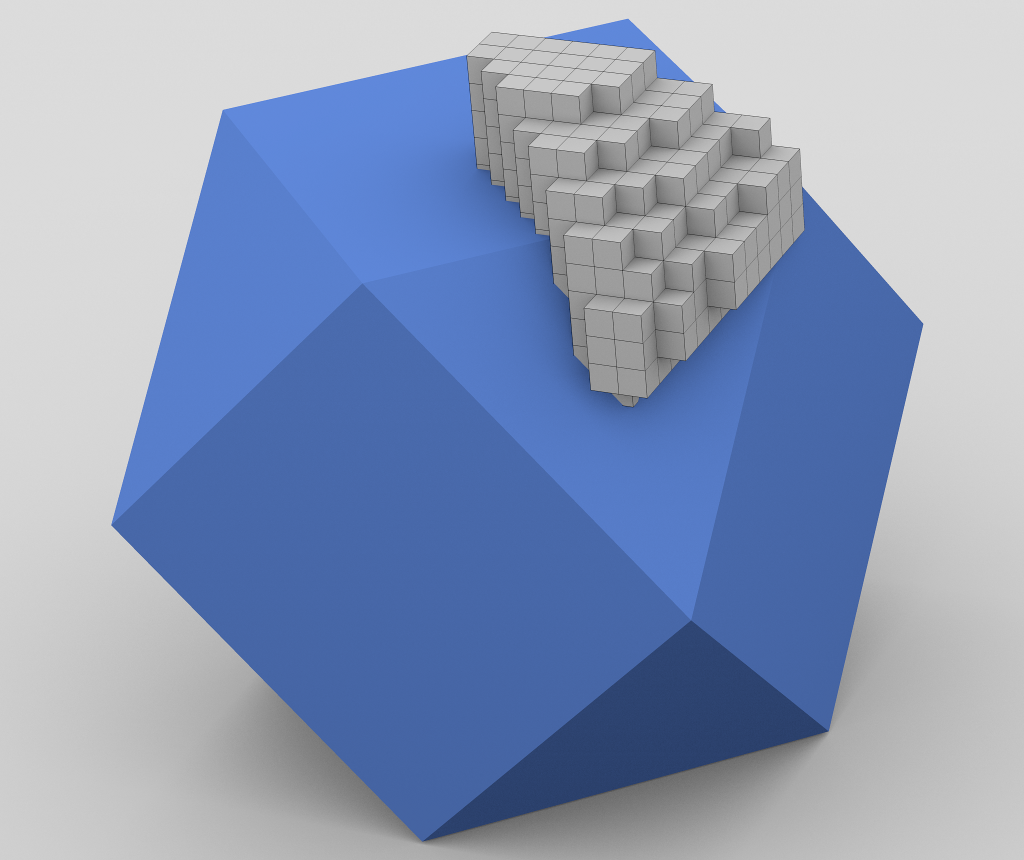
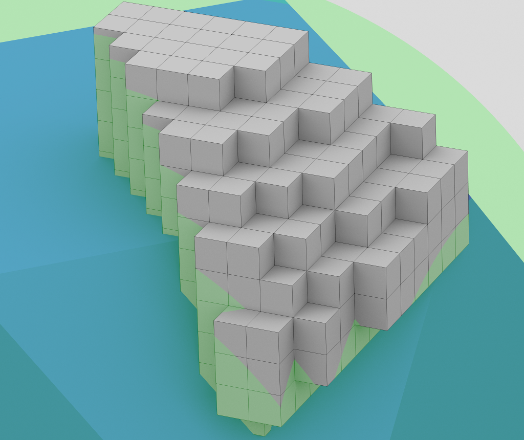
Figure 1. Here we have an initial cube partition for $\mathcal{D}^{\prime}$ where $\mathcal{K}$ is a regular tetrahedron so that $\mathcal{K}-\mathcal{K}$ is the cuboctahedron with circumradius $1$. We take $\alpha=1.02$ and $s(x)=\|x\|^{2}-1$. On the left we show the whole cuboctahedron and the partition. On the right we show the partition in detail; the unit sphere is also shown in green.

We then check that for every point in $\bigcup_{C\in\mathcal{C}}C$ the polynomial $\mathcal{F}[g]$ is nonpositive. We do that as follows.

First, for every cube $C\in\mathcal{C}$ we compute an upper bound of the norm of the gradient of $\mathcal{F}[g]$, a number $\nu_{C}$ such that

(15) $$\|\nabla\mathcal{F}[g](x)\|\leq\nu_{C}$$

for all $x\in C$. This is easy to do with interval arithmetic. We have the coefficients of $\mathcal{F}[g]$ represented by intervals. A cube $C=[x_{1},y_{1}]\times[x_{2},y_{2}]\times[x_{3},y_{3}]$ is the product of three intervals. We then only have to compute $\nabla\mathcal{F}[g]([x_{1},y_{1}],[x_{2},y_{2}],[x_{3},y_{3}])$ using interval arithmetic. This will give us a vector of intervals $([l_{1},u_{1}],[l_{2},u_{2}],[l_{3},u_{3}])$ such that for all $(x_{1},x_{2},x_{3})\in C$ we have

$$(l_{1},l_{2},l_{3})\leq\nabla\mathcal{F}[g](x_{1},x_{2},x_{3})\leq(u_{1},u_{2},u_{3}).$$

From this it is easy to compute a number $\nu_{C}$ satisfying (15).

Next, for a fixed integer $N\geq 1$, say, we uniformly divide each side of the cube $C$ into $N$ intervals, obtaining a grid of points inside of $C$. In other words, if $x_{C}$ is the lower-left corner of $C$, we consider the set of points

$$C_{N}=\{\,x_{C}+(a,b,c)\delta/N:0\leq a,b,c\leq N,\,a,b,c\in\mathbb{N}\,\}.$$

At least one point of $C$ belongs to $\mathcal{D}^{\prime}$, and hence at least one point of $C_{N}$ is not in $\alpha(\mathcal{K}^{\circ}-\mathcal{K}^{\circ})$. Let then $d(C,N)$ be the maximum minimum distance from any point of $C\setminus\alpha(\mathcal{K}^{\circ}-\mathcal{K}^{\circ})$ to a point of $C_{N}\setminus\alpha(\mathcal{K}^{\circ}-\mathcal{K}^{\circ})$ and let

$$\mu(C,N)=\max\{\,\mathcal{F}[g](x):x\in C_{N}\setminus\alpha(\mathcal{K}^{\circ}-\mathcal{K}^{\circ})\,\}.$$

If $\mu(C,N)>0$, then the function is not nonpositive in the required domain. We hope however that, for our choice of $\alpha>1$, we will have $\mu(C,N)<0$. Suppose that this is the case. Given $x\in C\setminus\alpha(\mathcal{K}^{\circ}-\mathcal{K}^{\circ})$, let $x^{\prime}$ be the point in $C_{N}\setminus\alpha(\mathcal{K}^{\circ}-\mathcal{K}^{\circ})$ closest to $x$. By the mean-value theorem we have that

$$|\mathcal{F}[g](x)-\mathcal{F}[g](x^{\prime})|\leq\nu_{C}\|x-x^{\prime}\|\leq\nu_{C}d(C,N).$$

So, if

(16) $$\nu_{C}d(C,N)\leq|\mu(C,N)|\leq|\mathcal{F}[g](x^{\prime})|,$$

then $\mathcal{F}[g](x)\leq 0$. Checking condition (16) for all $x^{\prime}\in C_{N}\setminus\alpha(\mathcal{K}^{\circ}-\mathcal{K}^{\circ})$ gives us a sufficient condition that allows us to conclude that $\mathcal{F}[g](x)\leq 0$ for all $x\in C\setminus\alpha(\mathcal{K}^{\circ}-\mathcal{K}^{\circ})$.

We still have to estimate $d(C,N)$, but that is a simple matter. There are two cases. If $C\cap\alpha(\mathcal{K}^{\circ}-\mathcal{K}^{\circ})\neq\emptyset$, then $d(C,N)\leq(\delta/N)\sqrt{3}$; if not, then $d(C,N)\leq(\delta/(2N))\sqrt{3}$.

So our strategy is to process each cube in $\mathcal{C}$. For each cube, we start with $N=2$ and check if that is enough to conclude that the function is nonpositive in the cube. If not, then we increase $N$. Once all cubes have been processed, we know that the function is nonpositive everywhere in the domain. Finally, notice that we always use interval arithmetic to perform all computations, thus obtaining rigorous results at the end, once the procedure terminates.

There is only one extra issue that is conceptually simple but that makes things technically harder. Computing with interval arithmetic is very slow, and hence if too many cubes would require dense grids (say, with hundreds of points per side), the computation would take several months. The size of the grid required by a cube is however directly proportional to the upper bound on the norm of the gradient, which is better the smaller the cube is. So, by taking smaller $\delta$, we can improve on the grid sizes. But by changing $\delta$ globally, we increase the total number of cubes, possibly slowing down the total computation time.

A better strategy is as follows: if the grid size required by a cube is greater than a certain threshold (we use $30$), then we split the cube at its center creating eight new cubes and keeping only those that intersect the domain. Then we process the resulting cubes instead, which are smaller and therefore lead to better grid sizes. This splitting process is carried out recursively, up to a certain maximum depth.

Finally, when one estimates the required grid size it may happen that, from one iteration to another, the grid size $N$ is increased only slightly. This should be avoided, since computing the function is quite expensive. So our approach is as follows: first, we carry out the whole verification procedure using double-precision floating-point arithmetic for function evaluation, but not for the other computations. This is quite fast, finishing in a few hours. Then we use the estimated grid size for each cube in a checking routine that remakes all calculations using interval arithmetic.

6.3. Further implementation details

Table 6 contains the list of bounds we computed and rigorously verified using the approach described in this section.

The solutions, as well as the verification scripts and programs, can be found as ancillary files from the arXiv.org e-print archive.

Body	Upper bound	Factor $\alpha$
Regular octahedron ($B_{3}^{1}$)	$0.972912750$	$1.001$
$B_{3}^{3}$	$0.823611150$	$1.002$
$B_{3}^{4}$	$0.874257405$	$1$
$B_{3}^{5}$	$0.922441815$	$1.005$
$B_{3}^{6}$	$0.933843309$	$1$
Regular tetrahedron	$0.374568355$	$1.02$
Truncated cube	$0.984519783$	$1.003$
Truncated tetrahedron	$0.729209804$	$1.023$

Table 6. List of rigorous bounds together with the factor $\alpha$ we needed in the verification.

The procedure to verify the SOS constraints was implemented as a Sage [46] script verify.sage and runs in Sage 6.2; see the documentation file README_SOSChecking. The approach to test that the function is nonpositive in the domain was implemented as a C++11 program called checker using the MPFI library [39] for interval arithmetic. Verification time was in all but one case under $2$ days; in the case of the regular octahedron it took several weeks. More documentation of the C++11 program can be found in README_SampleChecking and a description of the classes in docu.pdf.

It is interesting to observe that the polynomials $\mathcal{F}[g]$ obtained from the solutions to the semidefinite programs we consider provide interesting low degree polynomial approximations of the Minkowski difference $\mathcal{K}-\mathcal{K}$; We used $d=13$ in our computations, so that $g$ and $\mathcal{F}[g]$ have degree $26$. Figure 2 shows the cuboctahedron, which is the Minkowski difference of two regular tetrahedra, and the region $\{\,x\in\mathbb{R}^{3}:\mathcal{F}[g](x)\geq 0\,\}$, where $g$ is given by the solution to our problem for the tetrahedron. Notice how the region approximates the cuboctahedron. In fact, the upper bounds we computed are also bounds for translative packings of the nonconvex bodies determined by these polynomial approximations.

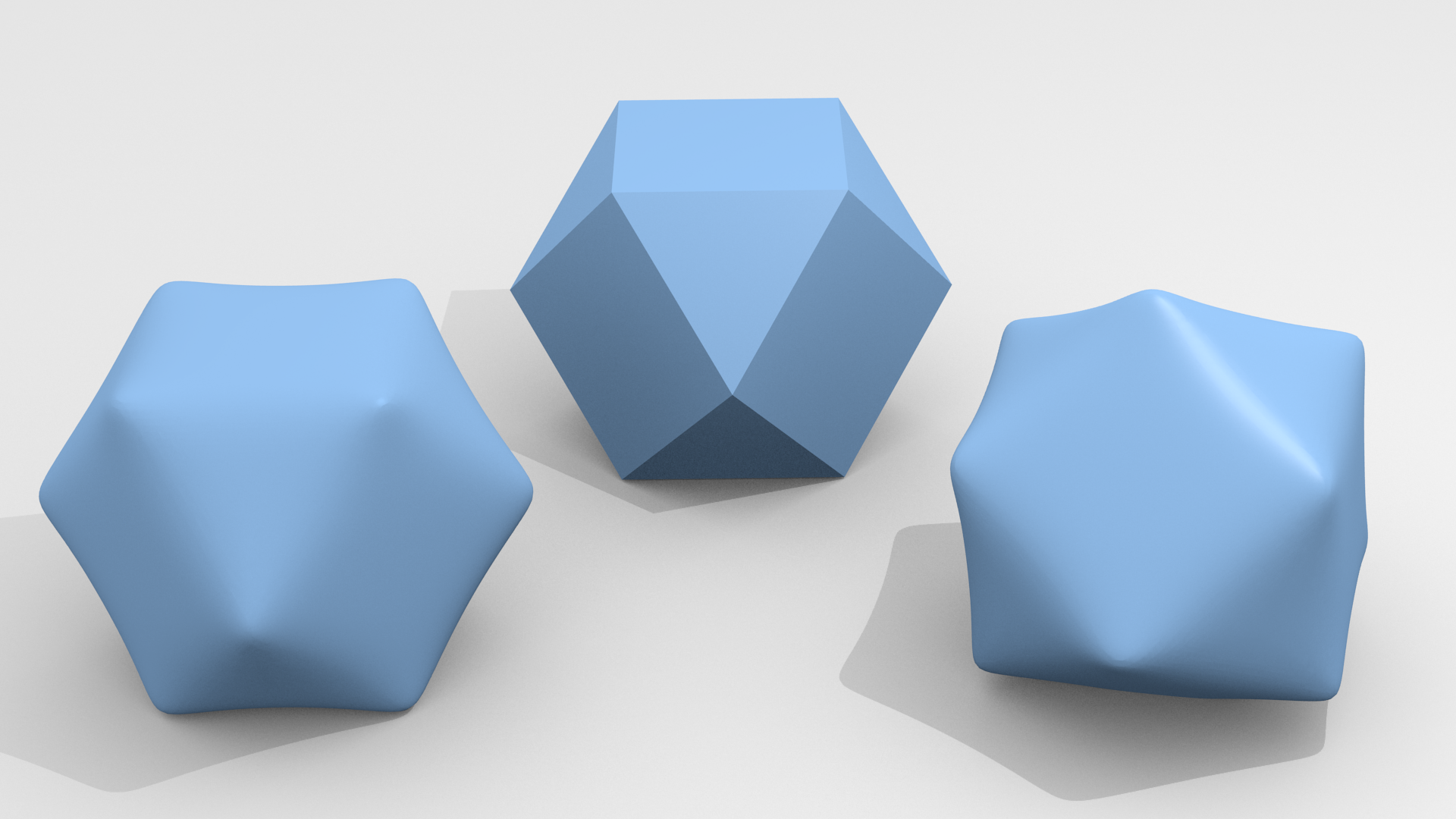
Figure 2. The cuboctahedron (center) with two rotations of the set $\{\,x\in\mathbb{R}^{3}:\mathcal{F}[g](x)\geq 0\,\}$, where $g$ is the polynomial given by the solution to our problem for the regular tetrahedron.

References

- [1] G.E. Andrews, R. Askey, and R. Roy, Special Functions, Encyclopedia of Mathematics and its Applications 71, Cambridge University Press, Cambridge, 1999.
- [2] C. Bachoc, D.C. Gijswijt, A. Schrijver, and F. Vallentin, Invariant semidefinite programs, pp. 219–269 in: Handbook on Semidefinite, Conic and Polynomial Optimization (M.F. Anjos, J.B. Lasserre (ed.)), International Series in Operations Research & Management Science 166, Springer, New York, 2012 (http://arxiv.org/abs/1007.2905)
- [3] U. Betke and M. Henk, Densest lattice packings of -polytopes, Comput. Geom. 16 (2000), 157–186. (http://arxiv.org/abs/math/9909172)
- [4] G. Blekherman, P.A. Parrilo, and R.R. Thomas, Semidefinite optimization and convex algebraic geometry, MOS-SIAM Series on Optimization 13, SIAM, Philadelphia, 2013.
- [5] E.R. Chen, M. Engel, and S.C. Glotzer, Dense crystalline dimer packings of regular tetrahedra, Discrete & Computational Geometry 44 (2010), 253–280. (http://arxiv.org/abs/1001.0586)
- [6] H. Cohn and N.D. Elkies, New upper bounds on sphere packings I, Ann. of Math. 157 (2003), 689–714. (http://arxiv.org/abs/math/0110009)
- [7] H. Cohn and A. Kumar, Universally optimal distribution of points on spheres, J. Amer. Math. Soc 20 (2007), 99–148. (http://arxiv.org/abs/math/0607446)
- [8] H. Cohn, A. Kumar, S.D. Miller, D. Radchenko, and M.S. Viazovska, The sphere packing problem in dimension , arXiv:1603.06518 [math.NT], 12 pages. (http://arxiv.org/abs/1603.06518)
- [9] H. Cohn and S.D. Miller, Some properties of optimal functions for sphere packing in dimensions and , arXiv:1603.04759 [math.MG], 23 pages. (http://arxiv.org/abs/1603.04759)
- [10] H. Cohn and Y. Zhao, Sphere packing bounds via spherical codes, Duke Math. J. 163 (2014), 1965–2002.
- [11] P.F. Damasceno, M. Engel, and S.C. Glotzer, Crystalline assemblies and densest packings of a family of truncated tetrahedra and the role of directional entropic forces, ACS Nano 6 (2012), 609–614. (http://arxiv.org/abs/1109.1323)
- [12] J.P. D’Angelo, Inequalities from Complex Analysis, Carus Mathematical Monographs 28, Mathematical Association of America, Washington, 2002.
- [13] J.P. D’Angelo, Hermitian analogues of Hilbert’s 17th problem, Adv. Math. 226 (2011), 4607–4637. (http://arxiv.org/abs/1012.2479)
- [14] C.F. Dunkl, Cube group invariant spherical harmonics and Krawtchouk polynomials, Math. Z. 177 (1981), 561–577.
- [15] N.D. Elkies, A.M. Odlyzko, and J.A. Rush, On the packing densities of superballs and other bodies, Invent. math. 105 (1991), 613–639.
- [16] G. Fejes Tóth, F. Fodor, and V. Vígh, The packing density of the n-dimensional cross-polytope, Discrete & Computational Geometry 54 (2015), 182–194. (http://arxiv.org/abs/1503.04571)
- [17] K. Fujisawa, M. Fukuda, K. Kobayashi, M. Kojima, K. Nakata, M. Nakata, and M. Yamashita, SDPA (SemiDefinite Programming Algorithm) User’s Manual — Version 7.0.5, Research Report B-448, Dept. of Mathematical and Computing Sciences, Tokyo Institute of Technology, Tokyo, 2008, http://sdpa.sourceforge.net.
- [18] M. Gardner, Mathematical carnival, Mathematical Association of America, Washington, 1989.
- [19] K. Gatermann and P.A. Parrilo, Symmetry groups, semidefinite programs, and sums of squares, J. Pure Appl. Algebra 192 (2004), 95–128. (http://arxiv.org/abs/math/0211450)
- [20] C.F. Gauss, Untersuchung über die Eigenschaften der positiven ternären quadratischen Formen von Ludwig August Seeber, J. Reine Angew. Math. 20 (1840), 312–320.
- [21] J.-M. Goethals and J.J. Seidel, Cubature formulae, polytopes, and spherical designs, pp. 203–218 in: The geometric vein. The Coxeter Festschrift (C. Davis, B. Grünbaum, F.A. Sherk (ed.)), Springer, 1981.
- [22] J. de Graaf, R. van Roij, and M. Dijkstra, Dense regular packings of irregular nonconvex particles, Phys. Rev. Lett. 107 (2011), 155501, 5 pp.
- [23] S. Gravel, V. Elser, and Y. Kallus, Upper bound on the packing density of regular tetrahedra and octahedra, Discrete & Computational Geometry 46 (2011), 799–818. (http://arxiv.org/abs/1008.2830)
- [24] H. Groemer, Über die dichteste gitterförmige Lagerung kongruenter Tetraeder, Monatsh. Math. 66 (1962), 12–15.
- [25] T. Hales and S. Ferguson, The Kepler conjecture. The Hales-Ferguson proof. Including papers reprinted from Discrete Comput. Geom. 36 (2006), Edited by J.C. Lagarias. Springer, New York, 2011.
- [26] J. Hicks, A Poet with a Slide Rule: Piet Hein Bestrides Art and Science, Life Magazine, October 14, 1966, 55–66.
- [27] D.J. Hoylman, The densest lattice packing of tetrahedra, Bull. Amer. Math. Soc. 76 (1970), 135–137.
- [28] J.E. Humphreys, Reflection groups and Coxeter groups, Cambridge Studies in Advanced Mathematics 29, Cambridge University Press, Cambridge, 1992.
- [29] Y. Jiao, F.H. Stillinger, and S. Torquato, Optimal packings of superballs, Phys. Rev. E 79 (2009), 041309, 12 pp. (http://arxiv.org/abs/0902.1504)
- [30] Y. Jiao, F.H. Stillinger, and S. Torquato, Erratum: Optimal packings of superballs [Phys. Rev. E 79, 041309 (2009)], Phys. Rev. E 84 (2011), 069902.
- [31] Y. Jiao and S. Torquato, A packing of truncated tetrahedra that nearly fills all of space and its melting properties, J. Chem. Phys. 135 (2011), 151101. (http://arxiv.org/abs/1107.2300)
- [32] G.A. Kabatiansky and V.I. Levenshtein, Bounds for packings on a sphere and in space, Problems of Information Transmission 14 (1978), 1–17.
- [33] D. de Laat, F.M. de Oliveira Filho, and F. Vallentin, Upper bounds for packings of spheres of several radii, Forum Math. Sigma 2 (2014), e23 (42 pages). (http://arxiv.org/abs/1206.2608)
- [34] J.C. Lagarias and C. Zong, Mysteries in packing regular tetrahedra, Notices Amer. Math. Soc. 59 (2012), 1540–1549.
- [35] H. Minkowski, Dichteste gitterförmige Lagerung kongruenter Körper, Nachr. Ges. Wiss. Göttingen (1904), 311–355.
- [36] R. Ni, A.P. Gantapara, J. de Graaf, R. van Roij, and M. Dijkstra, Phase diagram of colloidal hard superballs: from cubes via spheres to octahedra, Soft Matter 8 (2012), 8826–8834. (http://arxiv.org/abs/1111.4357)
- [37] F.M. de Oliveira Filho and F. Vallentin, Computing upper bounds for packing densities of congruent copies of a convex body I, arXiv:1308.4893, 2013, 28pp. (http://arxiv.org/abs/1308.4893)
- [38] A. Pütz, Translative packings of convex bodies and finite reflection groups, Master’s Thesis, University of Cologne, 2016.
- [39] N. Revol and F. Rouillier, Motivations for an arbitrary precision interval arithmetic and the MPFI library, Reliable Computing 11 (2005), 275–290.
- [40] B. Reznick, Some concrete aspects of Hilbert’s 17th problem, pp. 251–272 in: Real algebraic geometry and ordered structures (Baton Rouge, LA, 1996), Contemp. Math 253, Amer. Math. Soc., Providence, 2000.
- [41] L. Rossi, S. Sacanna, W.T.M. Irvine, P.M. Chaikin, D.J. Pine, and A.P. Philipse, Cubic crystals from cubic colloids, Soft Matter 7 (2011), 4139–4142.
- [42] J.A. Rush and N.J.A. Sloane, An improvement to the Minkowski-Hlawka bound for packing superballs, Mathematika 34 (1987), 8–18.
- [43] J.-P. Serre, Linear Representations of Finite Groups, Graduate Texts in Mathematics 42, Springer-Verlag, New York-Heidelberg, 1977.
- [44] R.P. Stanley, Invariants of finite groups and their application to combinatorics, Bull. Amer. Math. Soc. (N.S.) 1 (1979), 475–511.
- [45] E.M. Stein and G.L. Weiss, Introduction to Fourier analysis on Euclidean spaces, Princeton Mathematical Series 3, Princeton University Press, Princeton, 1971.
- [46] W.A. Stein et al., Sage Mathematics Software (Version 6.2), The Sage Development Team, 2012, http://www.sagemath.org. (http://www.sagemath.org)
- [47] B. Sturmfels, Algorithms in invariant theory, Texts and Monographs in Symbolic Computation, Springer-Verlag, Vienna, 1993.
- [48] A. Terras, Fourier Analysis on Finite Groups and Applications, London Mathematical Society Student Texts 43, Cambridge University Press, 1999.
- [49] S. Torquato and Y. Jiao, Dense packings of the Platonic and Archimedean solids, Nature 460 (2009), 876–879. (http://arxiv.org/abs/0908.4107)
- [50] S. Torquato and Y. Jiao, Dense packings of polyhedra: Platonic and Archimedean solids, Phys. Rev. E 80 (2009), 041104, 31 pp.
- [51] M.S. Viazovska, The sphere packing problem in dimension , arXiv:1603.04246 [math.NT], 22 pages. (http://arxiv.org/abs/1603.04246)
- [52] G.M. Ziegler, Three mathematics competitions, pp. 195–206 in: An Invitation to Mathematics: From Competitions to Research (D. Schleicher and M. Lackmann (ed.)), Springer, Heidelberg, 2011.
- [53] C. Zong, On the translative packing densities of tetrahedra and cuboctahedra, Adv. Math. 260 (2014), 130–190. (http://arxiv.org/abs/1208.0420)