Observable Gravitational Waves From Kinetically Modified Non-Minimal Inflation

Abstract:

We consider Supersymmetric (SUSY) and non-SUSY models of chaotic inflation based on the simplest power-law potential with exponents $n=2$ and $4$. We propose a convenient non-minimal coupling to gravity and a non-minimal kinetic term which ensure, mainly for $n=4$, inflationary observables favored by the Bicep2/Keck Array and Planck results. Inflation can be attained for subplanckian inflaton values with the corresponding effective theories retaining the perturbative unitarity up to the Planck scale.

Published in  PoS PLANCK 2015, 095 (2015).

1 Introduction

Kinetically modified Non-minimal (chaotic) inflation (nMI) [1] is a variant of nMI which arises in the presence of a non-canonical kinetic term for the inflaton $\phi$ – apart from the non-minimal coupling $f_{R}(\phi)$ between $\phi$ and the Ricci scalar curvature, ${R}$ which is required by definition in any model of nMI [2]. In this talk we focus on inflationary models based on a synergy between $f_{R}$ and the inflaton potential $V_{\rm CI}$, which are selected [1, 3, 4] as follows

$$V_{\rm CI}(\phi)=\lambda^{2}\phi^{n}/2^{n/2}\>\>\>\>\>\>\mbox{and}\>\>\>\>\>\>f_{R}=1+c_{R}\phi^{n/2}\>\>\>\>\>\>\mbox{with}\>\>\>\>\>\>n=2,4\,.$$ (1)

Below, we first (in Sec. 1.1) briefly review the basic ingredients of nMI in a non-Supersymmetric (SUSY) framework and constrain the parameters of the models in Sec. 1.3 taking into account a number of observational and theoretical requirements described in Sec. 1.2. Then (in Sec. 1.4) we focus on the problem with perturbative unitarity that plagues [5, 6] these models at the strong coupling and motivate the form of $f_{\rm K}$ analyzed in our work.

Throughout the text, the subscript $,\chi$ denotes derivation with respect to (w.r.t) the field $\chi$, charge conjugation is denoted by a star (^∗) and we use units where the reduced Planck scale $m_{\rm P}=2.43\cdot 10^{18}~{}{\mbox{\rm GeV}}$ is set equal to unity.

1.1 Coupling non-Minimally the Inflaton to Gravity

The action of the inflaton $\phi$ in the Jordan frame (JF), takes the form:

$${\sf S}=\int d^{4}x\sqrt{-\mathfrak{g}}\left(-\frac{f_{R}}{2}{R}+\frac{f_{\rm K}}{2}g^{\mu\nu}\partial_{\mu}\phi\partial_{\nu}\phi-V_{\rm CI}(\phi)\right).$$ (2)

where $\mathfrak{g}$ is the determinant of the background Friedmann-Robertson-Walker metric, $g^{\mu\nu}$ with signature $(+,-,-,-)$, $\langle{f_{R}}\rangle\simeq 1$ to guarantee the ordinary Einstein gravity at low energy and we allow for a kinetic mixing through the function $f_{\rm K}(\phi)$. By performing a conformal transformation [3] according to which we define the Einstein frame (EF) metric $\widehat{g}_{\mu\nu}=f_{R}\,g_{\mu\nu}$ we can write ${\sf S}$ in the EF as follows

$${\sf S}=\int d^{4}x\sqrt{-\widehat{\mathfrak{g}}}\left(-\frac{1}{2}\widehat{{R}}+\frac{1}{2}\widehat{g}^{\mu\nu}\partial_{\mu}\widehat{\phi}\partial_{\nu}\widehat{\phi}-\widehat{V}_{\rm CI}(\widehat{\phi})\right),$$ (3a)

where hat is used to denote quantities defined in the EF. We also introduce the EF canonically normalized field, $$\widehat{\phi} \widehat{V}_{\rm CI}$$, and potential, , defined as follows:

$$\frac{d\widehat{\phi}}{d\phi}=J=\sqrt{\frac{f_{\rm K}}{f_{R}}+{3\over 2}\left({f_{R,\phi}\over f_{R}}\right)^{2}}\>\>\>~{}\mbox{and}\>\>\>~{}\widehat{V}_{\rm CI}=\frac{V_{\rm CI}}{f_{R}^{2}}\,,$$ (3b)

where the symbol $,\phi$ as subscript denotes derivation w.r.t the field $\phi$. Plugging Eq. (1) into Eq. (3b), we obtain

$$J^{2}=\frac{f_{\rm K}}{f_{R}}+\frac{3n^{2}c_{R}^{2}\phi^{n-2}}{8f_{R}^{2}}\>\>\>\>\>\>~{}~{}\mbox{and}\>\>\>\>\>\>~{}\widehat{V}_{\rm CI}=\frac{\lambda^{2}\phi^{n}}{2^{n/2}f_{R}^{2}}.$$ (4)

In the pure nMI [2, 3, 4] we take $f_{\rm K}=1$ and, for $c_{R}\gg 1$, we infer from Eq. (3b), that $f_{R}$ determines the relation between $\widehat{\phi}$ and $\phi$ and controls the shape of $\widehat{V}_{\rm CI}$ affecting thereby the observational predictions – see below.

1.2 Inflationary Observables – Constraints

A model of nMI can be qualified as successful, if it can become compatible with the following observational and theoretical requirements:

1.2.1

The number of e-foldings ${\widehat{N}_{\star}}$ that the scale $k_{\star}=0.05/{\rm Mpc}$ experiences during this nMI must to be enough for the resolution of the horizon and flatness problems of standard Big Bang, i.e., [7]

$${\widehat{N}_{\star}}=\int_{\widehat{\phi}_{\rm f}}^{\widehat{\phi}_{\star}}d\widehat{\phi}\frac{\widehat{V}_{\rm CI}}{\widehat{V}_{\rm CI,\widehat{\phi}}}\simeq 55,$$ (5)

where $\phi_{\star}~{}[\widehat{\phi}_{\star}]$ are the value of $\phi~{}[\widehat{\phi}]$ when $k_{\star}$ crosses the inflationary horizon. Also $\phi_{\rm f}~{}[\widehat{\phi}_{\rm f}]$ is the value of $\phi~{}[\widehat{\phi}]$ at the end of nMI, which can be found, in the slow-roll approximation, from the condition

$${\footnotesize\sf max}\{\widehat{\epsilon}(\phi_{\rm f}),|\widehat{\eta}(\phi_{\rm f})|\}=1,\>\>\>~{}\mbox{where}$$

$$\widehat{\epsilon}={1\over 2}\left(\frac{\widehat{V}_{\rm CI,\widehat{\phi}}}{\widehat{V}_{\rm CI}}\right)^{2}={1\over 2J^{2}}\left(\frac{\widehat{V}_{\rm CI,\phi}}{\widehat{V}_{\rm CI}}\right)^{2}\>\>\>\mbox{and}\>\>\>\widehat{\eta}=\frac{\widehat{V}_{\rm CI,\widehat{\phi}\widehat{\phi}}}{\widehat{V}_{\rm CI}}={1\over J^{2}}\left(\frac{\widehat{V}_{\rm CI,\phi\phi}}{\widehat{V}_{\rm CI}}-\frac{\widehat{V}_{\rm CI,\phi}}{\widehat{V}_{\rm CI}}{J_{,\phi}\over J}\right)\cdot$$ (6)

It is evident from the formulas above that non trivial modifications on $f_{\rm K}$ and thus to $J$ may have an pronounced impact on the parameters above modifying thereby the inflationary observables too.

1.2.2

The amplitude $A_{\rm s}$ of the power spectrum of the curvature perturbation generated by $\phi$ at $k_{\star}$ has to be consistent with data [7], i.e.,

$$\sqrt{A_{\rm s}}=\>\frac{1}{2\sqrt{3}\,\pi}\;\frac{\widehat{V}_{\rm CI}(\widehat{\phi}_{\star})^{3/2}}{|\widehat{V}_{\rm CI,\widehat{\phi}}(\widehat{\phi}_{\star})|}={1\over 2\pi}\,\sqrt{\frac{\widehat{V}_{\rm CI}(\phi_{\star})}{6\widehat{\epsilon}_{\star}}}\simeq 4.627\cdot 10^{-5},$$ (7)

where the variables with subscript $\star$ are evaluated at $\phi=\phi_{\star}$.

1.2.3

The remaining inflationary observables (the spectral index $n_{\rm s}$, its running $a_{\rm s}$, and the tensor-to-scalar ratio $r$) – estimated through the relations:

$$\mbox{\footnotesize\sf(a)}\>\>n_{\rm s}=\>1-6\widehat{\epsilon}_{\star}\ +\ 2\widehat{\eta}_{\star},\>\>\>~{}\mbox{\footnotesize\sf(b)}\>\>a_{\rm s}=\frac{2}{3}\left(4\widehat{\eta}^{2}-(n_{\rm s}-1)^{2}\right)-2\widehat{\xi}_{\star}\>\>\>~{}\mbox{and}\>\>\>~{}\mbox{\footnotesize\sf(c)}\>\>r=16\widehat{\epsilon}_{\star}\,,$$ (8)

with $\widehat{\xi}={\widehat{V}_{\rm CI,\widehat{\phi}}\widehat{V}_{\rm CI,\widehat{\phi}\widehat{\phi}\widehat{\phi}}/\widehat{V}_{\rm CI}^{2}}$ – have to be consistent with the data [7], i.e.,

$$\mbox{\footnotesize\sf(a)}\>\>n_{\rm s}=0.968\pm 0.009\>\>\>~{}\mbox{and}\>\>\>~{}\mbox{\footnotesize\sf(b)}\>\>r\leq 0.12,$$ (9)

at 95$\%$ confidence level (c.l.) – pertaining to the $\Lambda$CDM$+r$ framework with $|a_{\rm s}|\ll 0.01$. Although compatible with Eq. (9b) the present combined Planck and Bicep2/Keck Array results [8] seem to favor $r$’s of order $0.01$ since $r=0.048^{+0.035}_{-0.032}$ at 68$\%$ c.l. has been reported.

1.2.4

The effective theory describing nMI has to remains valid up to a UV cutoff scale $\Lambda_{\rm UV}$ to ensure the stability of our inflationary solutions, i.e.,

$$\mbox{\footnotesize\sf(a)}\>\>\widehat{V}_{\rm CI}(\phi_{\star})^{1/4}\leq\Lambda_{\rm UV}\>\>\>~{}\mbox{and}\>\>\>~{}\mbox{\footnotesize\sf(b)}\>\>\phi_{\star}\leq\Lambda_{\rm UV}.$$ (10)

It is expected that $\Lambda_{\rm UV}\simeq m_{\rm P}$, contrary to the pure nMI with $c_{R}\gg 1$ where $\Lambda_{\rm UV}\ll m_{\rm P}$ – see Sec. 1.4.

1.3 The Two Regimes of Synergistic nMI

The models of nMI based on Eq. (1) exhibit the following two regimes:

1.3.1

The weak $c_{R}$ regime with $c_{R}\leq 1$. In this case from Eq. (3b) we find $J\simeq 1/f_{R}$ and applying Eqs. (5) and (6), the slow-roll parameters and ${\widehat{N}_{\star}}$ read

$$\widehat{\epsilon}\simeq\frac{n^{2}}{2\phi^{2}f_{R}},\>\>\>\widehat{\eta}\simeq 2\left(1-\frac{1}{n}\right)\widehat{\epsilon}-\frac{4+n}{2n}c_{R}\phi^{\frac{n}{2}}\widehat{\epsilon}\,\>\>\>\>\>\>\mbox{and}\>\>\>\>\>\>{\widehat{N}_{\star}}\simeq\frac{\phi_{\star}^{2}}{2n}\cdot$$ (11)

Imposing the condition of Eq. (6) and solving then the latter equation w.r.t $\phi_{*}$ we arrive at

$$\phi_{\rm f}\simeq n/\sqrt{2}\>\>\>\>\>\>\mbox{and}\>\>\>\>\>\>\phi_{\star}\simeq\sqrt{2n{\widehat{N}_{\star}}}\,.$$ (12)

Inflation is attained, thus, only for $\phi>1$. On the other hand, Eq. (7) implies

$$\lambda=\sqrt{6A_{\rm s}f_{n\star}}\pi n^{(2-n)/4}/{\widehat{N}_{\star}}^{(2+n)/4}\,,$$ (13)

where $f_{n\star}=f_{R}(\phi_{\star})=1+c_{R}(2n{\widehat{N}_{\star}})^{n/4}$. Applying Eq. (8) we find that the inflationary observables are $c_{R}$-dependent and can be marginally consistent with Eq. (9) – see Sec. 3.2. Indeed,

$$n_{\rm s}=1-\left(4+n+n/f_{n\star}\right)/4{\widehat{N}_{\star}},\>\>\>r=4n/f_{n\star}{\widehat{N}_{\star}},\>\>\>~{}~{}~{}~{}~{}~{}~{}~{}~{}~{}$$ (14a)

$$a_{\rm s}=\big{(}n^{2}-n(n+4)f_{n\star}-4(n+4)f_{n\star}^{2}\big{)}/16f_{n\star}^{2}{\widehat{N}_{\star}}^{2}\,.~{}~{}~{}$$ (14b)

In the limit $c_{R}\rightarrow 0$ or $f_{n\star}\rightarrow 1$ the results of the simplest power-law chaotic inflation – with $f_{R}=f_{\rm K}=1$ and $V_{\rm CI}$ given in Eq. (1) – are recovered. These are by now disfavored by Eq. (9).

1.3.2

The strong $c_{R}$ regime with $c_{R}\gg 1$. In this case, from Eq. (3b) we find

$$J\simeq{\sqrt{3}nc_{R}\phi^{n/2-1}/2\sqrt{2}f_{R}}\>\>\>\>\>\>\mbox{and}\>\>\>\>\>\>\widehat{V}_{\rm CI}\simeq\lambda^{2}/2^{n/2}c_{R}^{2}.\>\>$$ (15)

We observe that $\widehat{V}_{\rm CI}$ exhibits an almost flat plateau. From Eqs. (5) and (6) we find

$$\widehat{\epsilon}\simeq{4/3c_{R}^{2}\phi^{n}},\>\>\>\widehat{\eta}\simeq-{4/3c_{R}\phi^{n/2}}\>\>\>\>\>\>\mbox{and}\>\>\>\>\>\>{\widehat{N}_{\star}}\simeq{3c_{R}\phi_{*}^{n/2}/4}\,.$$ (16)

Therefore, $\phi_{\rm f}$ and $\phi_{\star}$ are found from the condition of Eq. (6) and the last equality above, as follows

$$\phi_{\rm f}=\mbox{\sf\footnotesize max}\{(4/3c_{R}^{2})^{1/n},(4/3c_{R})^{2/n}\}\>\>\>\>\>\>\mbox{and}\>\>\>\>\>\>\phi_{\star}=(4{\widehat{N}_{\star}}/3c_{R})^{2/n}.$$ (17)

Consequently, nMI can be achieved even with subplanckian $\phi$ values for $c_{R}\gtrsim(4{\widehat{N}}_{*}/3)^{2/n}$. Also the normalization of Eq. (7) implies the following relation between $c_{R}$ and $\lambda$

$$A^{1/2}_{\rm s}\simeq\left.2^{-(10+n)/4}\frac{\lambda c_{R}\phi^{n}}{\pi f_{R}}\right|_{\phi=\phi_{\star}}\>\>\>\Rightarrow\>\>\>\lambda\simeq\frac{3\cdot 2^{n/4}}{{\widehat{N}_{\star}}}\sqrt{2A_{\rm s}}\;\pi\;c_{R}\,.$$ (18)

From Eq. (8) we obtain the $c_{R}$-independent values for the observables:

$$n_{\rm s}\simeq 1-{2/{\widehat{N}_{\star}}}\simeq 0.965,\>\>\>a_{\rm s}\simeq{-2/{\widehat{N}_{\star}}^{2}}\simeq-6.4\cdot 10^{-4}\>\>\>\>\>\>\mbox{and}\>\>\>\>\>\>r\simeq{12/{\widehat{N}_{\star}}^{2}}\simeq 4\cdot 10^{-3},$$ (19)

which are in agreement with Eq. (9), although with low enough $r$ values.

1.4 The Ultraviolet (UV) Cut-off Scale

In the highly predictive regime with large $c_{\rm K}$, the models violate perturbative unitarity for $n>2$. To see this we analyze the small-field behavior of the theory in order to extract the UV cut-off scale $\Lambda_{\rm UV}$. The result depends crucially on the value of $J$ in Eq. (3b) in the vacuum, $\langle{\phi}\rangle=0$. Namely we have

$$\langle{J}\rangle=\begin{cases}\sqrt{3/2}c_{R}\>\>&\mbox{for}\>\>n=2,\\ 1\>\>&\mbox{for}\>\>n\neq 2\,.\end{cases}$$ (20)

For $n=2$ and any $c_{R}$ we obtain $\widehat{\phi}\neq\phi$. Expanding the second and third term of ${\sf S}$ in the right-hand side of Eq. (3a) about $\langle{\phi}\rangle=0$ in terms of $\widehat{\phi}$ we obtain:

$$J^{2}\dot{\phi}^{2}=\left(1-\sqrt{\frac{8}{3}}{\widehat{\phi}}+2{\widehat{\phi}^{2}}-\cdots\right)\dot{}\widehat{\phi}^{2}\>\>\>\>\>\>\mbox{and}\>\>\>\>\>\>\widehat{V}_{\rm CI}=\frac{\lambda^{2}\widehat{\phi}^{2}}{3c_{R}^{2}}\left(1-\sqrt{\frac{8}{3}}\widehat{\phi}+2\widehat{\phi}^{2}-\cdots\right).$$ (21)

As a consequence $\Lambda_{\rm UV}=m_{\rm P}$ since the expansions above are $c_{R}$ independent. On the contrary, for $n>2$ we have $\widehat{\phi}=\phi$ and the expansions of the same terms in Eq. (3a) are $c_{R}$ dependent:

$$J^{2}\dot{\phi}^{2}=\left(1-c_{R}\widehat{\phi}^{\frac{n}{2}}+\frac{3n^{2}}{8}c_{R}^{2}\widehat{\phi}^{n-2}+c_{R}^{2}\widehat{\phi}^{n}-\cdots\right)\dot{}\widehat{\phi}^{2};$$ (22a)

$$\widehat{V}_{\rm CI}=\frac{\lambda^{2}\widehat{\phi}^{n}}{2}\left(1-2c_{R}\widehat{\phi}^{\frac{n}{2}}+3c_{R}^{2}\widehat{\phi}^{n}-4c_{R}^{3}\widehat{\phi}^{\frac{3n}{2}}+\cdots\right)\cdot$$ (22b)

Since the term which yields the smallest denominator for $c_{R}>1$ is ${3n^{2}}c_{R}^{2}\widehat{\phi}^{n-2}/8$ we find [5, 6]:

$$\Lambda_{\rm UV}=m_{\rm P}/c_{R}^{2/(n-2)}\ll m_{\rm P}\,.$$ (23)

However, if we introduce a non-canonical kinetic mixing of the form

$$f_{\rm K}(\phi)=c_{\rm K}f_{R}^{m}\>\>\>\>\>\>\mbox{where}\>\>\>\>\>\>c_{\rm K}=(c_{R}/r_{{R}\rm K})^{4/n}\>\>\>\>\>\>\mbox{and}\>\>\>\>\>\>m\geq 0,$$ (24)

no problem with the perturbative unitarity emerges for $r_{{R}\rm K}\leq 1$, even if $c_{R}$ and/or $c_{\rm K}$ are large – the latter situation is expected if we wish to achieve efficient nMI with $\phi\leq 1$. E.g., for $m=0$ the expansions in Eqs. (22a) and (22b) can be rewritten replacing $c_{R}$ with $r_{{R}\rm K}$ and $\lambda$ with $\lambda/c_{\rm K}^{n/4}$ – similar expressions can be obtained for other $m$, too. In other words, the perturbative unitarity can be preserved up to $m_{\rm P}$ if we select a non-trivial $f_{\rm K}$ such that $\langle{J}\rangle\neq 1$. This requirement lets a functional uncertainty as regards the form of $f_{\rm K}$ during nMI which can be parameterized as shown in Eq. (24) given that $\langle{f_{R}}\rangle\simeq 1$ – see Sec. 1.1.

We below describe a possible formulation of this type of nMI in the context of Supergravity (SUGRA) – see Sec. 2 – and then, in Sec. 3, we analyze the inflationary behavior of these models. We conclude summarizing our results in Sec. 4.

2 Supergravity Embeddings

The models above – defined by Eqs. (1) and (24) – can be embedded in SUGRA if we use two gauge singlet chiral superfields $z^{\alpha}=\Phi,S$, with $\Phi$ (${\alpha}=1$) and $S$ (${\alpha}=2)$ being the inflaton and a “stabilizer” field respectively. The EF action for $z^{\alpha}$’s can be written as [9]

$${\sf S}=\int d^{4}x\sqrt{-\widehat{\mathfrak{g}}}\left(-\frac{1}{2}\widehat{{R}}\ +\ K_{{\alpha}{\bar{\beta}}}\widehat{g}^{\mu\nu}\partial_{\mu}z^{\alpha}\partial_{\nu}z^{*{\bar{\beta}}}-\widehat{V}\right)\,,$$ (25a)

where summation is taken over the scalar fields $$z^{\alpha} K K_{{\alpha}{\bar{\beta}}}=K_{,z^{\alpha}z^{*{\bar{\beta}}}} K^{{\alpha}{\bar{\beta}}}K_{{\bar{\beta}}\gamma}=\delta^{\alpha}_{\gamma} \widehat{V}$$, is the Kähler potential with and . Also is the EF F–term SUGRA potential given by

$$\widehat{V}=e^{K}\left(K^{{\alpha}{\bar{\beta}}}D_{\alpha}WD^{*}_{\bar{\beta}}W^{*}-3{|W|^{2}}\right),$$ (25b)

where $D_{\alpha}W=W_{,z^{\alpha}}+K_{,z^{\alpha}}W$ with $W$ being the superpotential. Along the inflationary track determined by the constraints

$$S=\Phi-\Phi^{*}=0,\>\>\>\mbox{or}\>\>\>s=\bar{s}={\theta}=0$$ (26)

Superfields	$S$	$\Phi$
$U(1)_{R}$	$1$	$0$
$U(1)$	$-1$	$2/n$

Table 1: Charge assignments of the superfields.

if we express $\Phi$ and $S$ according to the parametrization

$$\Phi=\>{\phi\,e^{i{\theta}}}/{\sqrt{2}}\>\>\>\>\>\>\mbox{and}\>\>\>\>\>\>S=\>(s+i\bar{s})/\sqrt{2}\,,$$ (27)

$V_{\rm CI}$ in Eq. (1) can be produced, in the flat limit, by

$$W=\lambda S\Phi^{n/2}.$$ (28)

The form of $W$ can be uniquely determined if we impose an $R$ and a global $U(1)$ symmetry with charge assignments shown in Table 1.

On the other hand, the derivation of $\widehat{V}_{\rm CI}$ in Eq. (4) via Eq. (25b) requires a judiciously chosen $K$. Namely, along the track in Eq. (26) the only surviving term in Eq. (25b) is

$$\widehat{V}_{\rm CI}=\widehat{V}({\theta}=s=\bar{s}=0)=e^{K}K^{SS^{*}}\,|W_{,S}|^{2}\,.$$ (29)

The incorporation $f_{R}$ in Eq. (1) and $f_{\rm K}$ in Eq. (24) dictates the adoption of a logarithmic $K$ [9] including the functions

$$F_{R}(\Phi)=1+2^{\frac{n}{4}}\Phi^{\frac{n}{2}}c_{R}\,,\>\>\>F_{\rm K}=(\Phi-\Phi^{*})^{2}\,\>\>\>\>\>\>\mbox{and}\>\>\>\>\>\>F_{S}={|S|^{2}}-k_{S}{|S|^{4}}\,.$$ (30)

Here, $F_{R}$ is an holomorphic function reducing to $f_{R}$, along the path in Eq. (26), $F_{\rm K}$ is a real function which assists us to incorporate the non-canonical kinetic mixing generating by $f_{\rm K}$ in Eq. (24), and $F_{S}$ provides a typical kinetic term for $S$, considering the next-to-minimal term for stability/heaviness reasons [9]. Indeed, $F_{\rm K}$ lets intact $\widehat{V}_{\rm CI}$, since it vanishes along the trajectory in Eq. (26), but it contributes to the normalization of $\Phi$. Taking for consistency all the possible terms up to fourth order, $K$ is written as

$$K_{1}=-3\ln\left(\frac{1}{2}\left(F_{R}+F_{R}^{*}\right)+\frac{c_{\rm K}}{3\cdot 2^{m+1}}\left(F_{R}+F_{R}^{*}\right)^{m}F_{\rm K}-\frac{1}{3}F_{S}+\frac{k_{\Phi}}{6}F_{\rm K}^{2}-\frac{k_{S\Phi}}{3}F_{\rm K}{|S|^{2}}\right)\,.~{}~{}~{}~{}~{}$$ (31a)

Alternatively, if we do not insist on a pure logarithmic $$K$$, we could also adopt the form

$$K_{2}=-3\ln\left(\frac{1}{2}\left(F_{R}+F_{R}^{*}\right)-\frac{1}{3}F_{S}\right)-\frac{c_{\rm K}}{2^{m}}\frac{F_{\rm K}}{\left(F_{R}+F_{R}^{*}\right)^{1-m}}\,\cdot$$ (31b)

Moreover, if we place $$F_{S} K$$ outside the argument of the logarithm similar results are obtained by the following ’s – not mentioned in Ref. [1]:

$$K_{3}=-2\ln\left(\frac{1}{2}\left(F_{R}+F_{R}^{*}\right)+\frac{c_{\rm K}}{2^{m+2}}\left(F_{R}+F_{R}^{*}\right)^{m}F_{\rm K}\right)+F_{S}\,,$$ (31c)

$$K_{4}=-2\ln\frac{F_{R}+F_{R}^{*}}{2}-\frac{c_{\rm K}}{2^{m}}\frac{F_{\rm K}}{\left(F_{R}+F_{R}^{*}\right)^{1-m}}+F_{S}\,.$$ (31d)

Note that for $m=0$ [$m=1$], $F_{R}$ and $F_{\rm K}$ in $K_{1}$ and $K_{3}$ [$K_{2}$ and $K_{4}$] are totally decoupled, i.e. no higher order term is needed. Also we use only integer prefactors for the logarithms avoiding thereby any relevant tuning – cf. Ref. [10]. Our models, for $c_{\rm K}\gg c_{R}$, are completely natural in the ’t Hooft sense because, in the limits $c_{R}\rightarrow 0$ and $\lambda\rightarrow 0$, the theory enjoys the enhanced symmetries

$$\Phi\rightarrow\ \Phi^{*},\>\Phi\rightarrow\ \Phi+c\>\>\>\>\>\>\mbox{and}\>\>\>\>\>\>S\rightarrow\ e^{i\alpha}S,$$ (32)

where $c$ is a real number. It is evident that our proposal is realized more attractively within SUGRA than within the non-SUSY set-up, since both $f_{\rm K}$ and $f_{R}$ originate from the same function $K$.

To verify the appropriateness of $K$’s in Eqs. (31a) – (31d), we can first remark that, along the trough in Eq. (26), these are diagonal with non-vanishing elements $K_{SS^{*}}$ and $K_{\Phi\Phi^{*}}=J^{2}$, where $J$ is given by Eq. (4) for $K=K_{i}$ and Eq. (4) replacing $3/8$ by $1/4$ for $K=K_{i+2}$. Substituting into Eq. (29) $K^{SS^{*}}=1/K_{SS^{*}}$ and $\exp K=1/f_{R}^{N}$, where

$$K_{SS^{*}}=\begin{cases}1/f_{R}\\ 1\end{cases}\mbox{and}\>\>\>\>N=\begin{cases}3\\ 2\end{cases}\mbox{for}\>\>\>\>\>\>K=\begin{cases}K_{i}\\ K_{i+2}\end{cases}\mbox{with}~{}~{}i=1,2,$$ (33)

we easily deduce that $\widehat{V}_{\rm CI}$ in Eq. (4) is recovered. If we perform the inverse of the conformal transformation described in Eqs. (3a) and (2) with frame function ${\Omega/N}=-e^{-{K}/{N}}$ we can easily show that $f_{R}=-\Omega/N$ along the path in Eq. (26). Note, finally, that the conventional Einstein gravity is recovered at the SUSY vacuum, $\langle{S}\rangle=\langle{\Phi}\rangle=0$, since $\langle{f_{R}}\rangle\simeq 1$.

Fields	Eingestates	Masses Squared
		Symbol	$K=K_{1}$	$K=K_{2}$	$K=K_{i+2}$
2 real scalars	$\widehat{\theta}$	$\widehat{m}_{\theta}^{2}$	$4\widehat{H}_{\rm CI}^{2}$	$6\widehat{H}_{\rm CI}^{2}$
1 complex scalar	$\widehat{s},\widehat{\bar{s}}$	$\widehat{m}_{s}^{2}$	$6\left(2k_{S}f_{R}-1/3\right)\widehat{H}_{\rm CI}^{2}$		$12k_{S}\widehat{H}_{\rm CI}^{2}$
$4$ Weyl spinors	$\widehat{\psi}_{\pm}$	$\widehat{m}^{2}_{\psi\pm}$	$3n^{2}\widehat{H}_{\rm CI}^{2}/2c_{\rm K}\phi^{2}f_{R}^{1+m}$

Table 2: Mass-squared spectrum for $K=K_{i}$ and $K=K_{i+2}$ ($i=1,2$) along the path in Eq. (2.2).

Defining the canonically normalized fields via the relations ${d\widehat{}\phi/d\phi}=\sqrt{K_{\Phi\Phi^{*}}}=J$, $\widehat{{\theta}}=J{\theta}\phi$ and $(\widehat{s},\widehat{\bar{s}})=\sqrt{K_{SS^{*}}}{(s,\bar{s})}$ we can verify that the configuration in Eq. (26) is stable w.r.t the excitations of the non-inflaton fields. Taking the limit $c_{\rm K}\gg c_{R}$ we find the expressions of the masses squared $\widehat{m}^{2}_{\chi^{\alpha}}$ (with $\chi^{\alpha}={\theta}$ and $s$) arranged in Table 2, which approach rather well the quite lengthy, exact formulas. From these expressions we appreciate the role of $k_{S}>0$ in retaining positive $\widehat{m}^{2}_{s}$. Also we confirm that $\widehat{m}^{2}_{\chi^{\alpha}}\gg\widehat{H}_{\rm CI}^{2}=\widehat{V}_{\rm CI0}/3$ for $\phi_{\rm f}\leq\phi\leq\phi_{\star}$. In Table 2 we display the masses $\widehat{m}^{2}_{\psi^{\pm}}$ of the corresponding fermions too with eignestates $\widehat{\psi}_{\pm}=(\widehat{\psi}_{\Phi}\pm\widehat{\psi}_{S})/\sqrt{2}$, defined in terms of $\widehat{\psi}_{S}=\sqrt{K_{SS^{*}}}\psi_{S}$ and $\widehat{\psi}_{\Phi}=\sqrt{K_{\Phi\Phi^{*}}}\psi_{\Phi}$, where $\psi_{\Phi}$ and $\psi_{S}$ are the Weyl spinors associated with $S$ and $\Phi$ respectively. Note, finally, that $\widehat{m}_{\chi^{\alpha}}\ll m_{\rm P}$, for any $\chi^{\alpha}$, contrary to similar cases [11] where the inflaton belongs to gauge non-singlet superfields.

Inserting the derived mass spectrum in the well-known Coleman-Weinberg formula, we can find the one-loop radiative corrections, $\Delta\widehat{V}_{\rm CI}$ to $\widehat{V}_{\rm CI}$. It can be verified that our results are immune from $\Delta\widehat{V}_{\rm CI}$, provided that the renormalization group mass scale $\Lambda$, is determined conveniently and $k_{S\Phi}$ and $k_{S}$ are confined to values of order unity.

3 Results

The present inflationary scenario depends on the parameters: $n,~{}m,~{}r_{{R}\rm K},~{}\lambda/c_{\rm K}^{n/4}$. Note that the two last combinations of parameters above replace $c_{\rm K}$, $c_{R}$ and $\lambda$. This is because, if we perform a rescaling $\phi=\tilde{}\phi/\sqrt{c_{\rm K}}$, Eq. (2) preserves its form replacing $\phi$ with $\tilde{}\phi$ and $f_{\rm K}$ with $f_{R}^{m}$ where $f_{R}$ and $V_{\rm CI}$ take, respectively, the forms

$$f_{R}=1+r_{{R}\rm K}\tilde{}\phi^{n/2}\>\>\>\>\>\>\mbox{and}\>\>\>\>\>\>V_{\rm CI}=\lambda^{2}\tilde{}\phi^{n}/2^{n/2}c_{\rm K}^{n/2},$$ (34)

which, indeed, depend only on $r_{{R}\rm K}$ and $\lambda^{2}/c_{\rm K}^{n/2}$. Imposing the restrictions of Sec. 1.2 we can delineate the allowed region of these parameters. Below we first extract some analytic expressions – see Sec. 3.1 – which assist us to interpret the exact numerical results presented in Sec. 3.2.

3.1 Analytic Results

Assuming $c_{\rm K}\gg c_{R}$, Eq. (3b) yields $J\simeq\sqrt{c_{\rm K}}/f_{R}^{(1-m)/2}$. Inserting the last one and $\widehat{V}_{\rm CI}$ from Eq. (1) in Eq. (6) we extract the slow-roll parameters for this model as follows – cf. Eq. (11):

$$\widehat{\epsilon}={n^{2}}/{2\phi^{2}c_{\rm K}f_{R}^{1+m}}\>\>\>\>\>\>\mbox{and}\>\>\>\>\>\>{\widehat{\eta}}=2\left(1-1/n\right)\widehat{\epsilon}-\left({4+n(1+m)}\right)c_{R}\phi^{n/2}\widehat{\epsilon}/{2n}\,.$$ (35)

Given that $\phi\ll 1$ and so $f_{R}\simeq 1$, nMI terminates for $\phi=\phi_{\rm f}$ found by the condition

$$\phi_{\rm f}\simeq\mbox{\footnotesize\sf max}\{{n/\sqrt{2c_{\rm K}}},\sqrt{(n-1)n/c_{\rm K}}\}\,,$$ (36)

in accordance with Eq. (6). Since $\phi_{\star}\gg\phi_{\rm f}$, from Eq. (5) we find

$${\widehat{N}_{\star}}=\frac{c_{\rm K}\phi_{\star}^{2}}{2n}\;{}_{2}F_{1}\left(-m,4/n;1+4/n;-c_{R}\phi_{\star}^{n/2}\right)=\begin{cases}{c_{\rm K}\phi_{\star}^{2}}/{2n}\>\>\>&\mbox{for}\>\>\>m=0,\\ (f_{R}^{1+m}-1)/8(1+m)r_{{R}\rm K}\>\>\>&\mbox{for}\>\>\>n=4,\end{cases}$$ (37)

where ${}_{2}F_{1}$ is the Gauss hypergeometric function. Concentrating on the cases with $m=0$ or $n=4$, we solve Eq. (37) w.r.t $\phi_{\star}$ with results

$$\phi_{\star}\simeq\begin{cases}\sqrt{2n{\widehat{N}_{\star}}/c_{\rm K}}\>\>\>&\mbox{for}\>\>\>\>\>\>m=0,\\ \sqrt{f_{m\star}-1}/\sqrt{r_{{R}\rm K}c_{\rm K}}\>\>\>&\mbox{for}\>\>\>\>\>\>n=4,\end{cases}$$ (38)

where $f_{m\star}^{1+m}=1+8(m+1)r_{{R}\rm K}{\widehat{N}_{\star}}$. In both cases there is a lower bound on $c_{\rm K}$, above which $\phi_{\star}<1$ and so, our proposal can be stabilized against corrections from higher order terms – e.g., for $n=4,m=1$ and $r_{{R}\rm K}=0.03$ we obtain $140\lesssim c_{\rm K}\lesssim 1.4\cdot 10^{6}$ for $3.3\cdot 10^{-4}\lesssim\lambda\lesssim 3.5$. The correlation between $\lambda$ and $c_{\rm K}^{n/4}$ can be found from Eq. (7). For $m=0$ this is given by Eq. (13) replacing $\lambda$ with $\lambda/c_{\rm K}^{n/4}$ and $c_{R}$ with $r_{{R}\rm K}$ in the definition of $f_{n\star}$. For $n=4$ we obtain

$$\lambda=16\sqrt{3A_{\rm s}}\,\pi\,c_{\rm K}\,r_{{R}\rm K}^{3/2}/(f_{m\star}-1)^{3/2}f_{m\star}^{(1+m)/2}\,.$$ (39)

As regards the inflationary observables, these are obviously given by Eqs. (14a) and (14b) for the trivial case with $m=0$. For $m\neq 0$, however, these are heavily altered. In particular, for $n=4$ we obtain

$$n_{\rm s}=1-8r_{{R}\rm K}\frac{m-1-(m+2)f_{m\star}}{(f_{m\star}-1)f_{m\star}^{1+m}},\>\>\>r=\frac{128r_{{R}\rm K}}{(f_{m\star}-1)f_{m\star}^{1+m}},$$ (40a)

$$\>\>\>a_{\rm s}=\frac{64r_{{R}\rm K}^{2}(1+m)(m+2)}{(f_{m\star}-1)^{2}f_{m\star}^{4(1+m)}}f_{m\star}^{2}\left(f_{m\star}^{2m}\left(\frac{1-m}{m+2}+\frac{2m-1}{m+1}f_{m\star}\right)-f_{m\star}^{2(1+m)}\right).~{}~{}~{}$$ (40b)

The formulae above is valid only for $r_{{R}\rm K}>0$ – see Eq. (38) – and is simplified [1] for low $m$’s.

3.2 Numerical Results

The conclusions obtained in Sec. 3.1 can be verified and extended to others $n$’s and $m$’s numerically. In particular, enforcing Eqs. (5) and (7) we can restrict $\phi_{\star}$ and $\lambda/c_{\rm K}^{n/4}$. Then we can compute the model predictions via Eq. (8), for any selected $m,n$ and $r_{{R}\rm K}$. The outputs, encoded as lines in the $n_{\rm s}-r_{0.002}$ plane, are compared against the observational data [7, 8] in Fig. 1 for $n=2$ (left panel) and $4$ (right panel) setting $m=0,1$ and $4$ – dashed, solid, and dot-dashed lines respectively. The variation of $r_{{R}\rm K}$ is shown along each line. To obtain an accurate comparison, we compute $r_{0.002}=16\widehat{\epsilon}(\phi_{0.002})$ where $\phi_{0.002}$ is the value of $\phi$ when the scale $k=0.002/{\rm Mpc}$, which undergoes $\widehat{N}_{0.002}=({\widehat{N}_{\star}}+3.22)$ e-foldings during nMI, crosses the inflationary horizon.

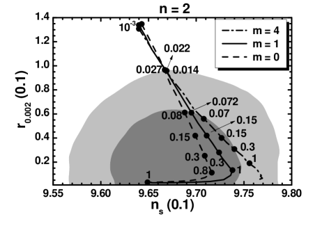
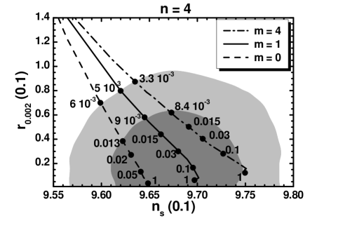
Figure 1: Allowed curves in the $n_{\rm s}-r_{0.002}$ plane for $n=2$ and $4$, $m=0$ (dashed lines), $m=1$ (solid lines), $m=4$ (dot-dashed lines), and various $r_{{R}\rm K}$’s indicated on the curves. The marginalized joint $68\%$ [$95\%$] regions from Planck, Bicep2/Keck Array and BAO data are depicted by the dark [light] shaded contours.

From the plots in Fig. 1 we observe that, for low enough $r_{{R}\rm K}$’s – i.e. $r_{{R}\rm K}=10^{-4}$ and $0.001$ for $n=4$ and $2$ –, the various lines converge to the $(n_{\rm s},r_{0.002})$’s obtained within the simplest models of chaotic inflation with the same $n$. At the other end, the lines for $n=4$ terminate for $r_{{R}\rm K}=1$, beyond which the theory ceases to be unitarity safe – as anticipated in Sec. 1.4 – whereas the $n=2$ lines approach an attractor value, comparable with the value in Eq. (19), for any $m$.

For $m=0$ we reveal the results of Sec. 1.3, i.e. the displayed lines are almost parallel for $r_{0.002}\geq 0.02$ and converge at the values in Eq. (19) – for $n=4$ this is reached even for $r_{{R}\rm K}=1$. Our estimations in Eqs. (14a) – (14b) are in agreement with the numerical results for $n=2$ and $r_{{R}\rm K}\lesssim 1$ or $n=4$ and $r_{{R}\rm K}\lesssim 0.05$. We observe that the $n=2$ line is closer to the central values in Eq. (9) whereas the $n=4$ one deviates from those.

For $m>0$ the curves change slopes w.r.t to those with $m=0$ and move to the right. As a consequence, for $n=4$ they span densely the 1-$\sigma$ ranges in Eq. (9) for quite natural $r_{{R}\rm K}$’s – e.g. $0.005\lesssim r_{{R}\rm K}\lesssim 0.1$ for $m=1$. It is worth mentioning that the requirement $r_{{R}\rm K}\leq 1$ (for $n=4$) provides a lower bound on $r_{0.002}$, which ranges from $0.004$ for $m=0$ to $0.015$ (for $m=4$). Therefore, our results are testable in the forthcoming experiments [12] hunting for primordial gravitational waves. Note, finally, that our findings in Eqs. (40a) – (40b) approximate fairly the numerical outputs for $0.003\lesssim r_{{R}\rm K}\leq 1$.

4 Conclusions

We reviewed the implementation of kinetically modified nMI in both a non-SUSY and a SUSY framework. The models are tied to the potential $V_{\rm CI}$ and the coupling function of the inflaton to gravity given in Eq. (1) and the non-canonical kinetic mixing in Eq. (24). This setting can be elegantly implemented in SUGRA too, employing the super-and Kähler potentials given in Eqs. (28) and (31a) – (31d). Prominent in this realization is the role of a shift-symmetric quadratic function $F_{\rm K}$ in Eq. (30) which remains invisible in the SUGRA scalar potential while dominates the canonical normalization of the inflaton. Using $m\geq 0$ and confining $r_{{R}\rm K}$ to the range $(3.3\cdot 10^{-3}-1)$, where the upper bound does not apply to the $n=2$ case, we achieved observational predictions which may be tested in the near future and converge towards the “sweet” spot of the present data – especially for $n=4$. These solutions can be attained even with subplanckian values of the inflaton requiring large $c_{\rm K}$’s and without causing any problem with the perturbative unitarity. It is gratifying, finally, that the most promising case of our proposal with $n=4$ can be studied analytically and rather accurately.

References

[1] C. Pallis, Phys. Rev. D 91, 123508 (2015) [arXiv:1503.05887].
[2] D. S. Salopek, J. R. Bond and J.M.
Bardeen, Phys. Rev. D 40, 1753 (1989);
F.L. Bezrukov
and M. Shaposhnikov, Phys. Lett. B 659, 703 (2008) [arXiv:0710.3755].
[3] C. Pallis, Phys. Lett. B 692, 287 (2010)
[arXiv:1002.4765];
C. Pallis and Q. Shafi,
Phys. Rev. D 86, 023523 (2012) [arXiv:1204.0252].
[4] R. Kallosh, A. Linde, and D. Roest,
Phys. Rev. Lett.112, 011303 (2014)
[arXiv:1310.3950].
[5] J.L.F. Barbon and J.R. Espinosa,
Phys. Rev. D 79, 081302 (2009) [arXiv:0903.0355];
C.P. Burgess,
H.M. Lee, and M. Trott, JHEP07, 007 (2010) [arXiv:1002.2730].
[6] A. Kehagias, A.M. Dizgah, and A. Riotto, Phys. Rev. D 89, 043527 (2014)
[arXiv:1312.1155].