On linear hypocoercive BGK models

Abstract

We study hypocoercivity for a class of linear and linearized BGK models for discrete and continuous phase spaces. We develop methods for constructing entropy functionals that prove exponential rates of relaxation to equilibrium. Our strategies are based on the entropy and spectral methods, adapting Lyapunov’s direct method (even for “infinite matrices” appearing for continuous phase spaces) to construct appropriate entropy functionals. Finally, we also prove local asymptotic stability of a nonlinear BGK model.

1 Introduction

This paper is concerned with the large time behavior of linear BGK models (named after the physicists Bhatnagar-Gross-Krook BGK54 ) for a phase space density $f(x,v,t)$; $x,\,v\in\mathbb{R}^{d}$, satisfying the kinetic evolution equation

$$f_{t}+v\cdot\nabla_{x}f-\nabla_{x}V\cdot\nabla_{v}f=\mathbf{Q}f:=M_{T(t)}(v)\,\int_{\mathbb{R}^{d}}f(x,v,t)\,\,\operatorname{d}\!v-f(x,v,t)\,,\quad t\geq 0\,,$$ (1.1)

with some given confinement potential $V(x)$ and where $M_{T}$ denotes the normalized Maxwellian at some temperature $T$:

$$M_{T}(v)=(2\pi T)^{-d/2}e^{-|v|^{2}/2T}\ .$$

We assume that the initial condition is normalized as

$$\int_{\mathbb{R}^{d}\times\mathbb{R}^{d}}f(x,v,0)\,{\rm d}x{\rm d}v=1\ ,$$

and this normalization persists under the flow of (1.1). The function $T(t)$ is defined so that the energy is conserved:

$$\int_{\mathbb{R}^{d}\times\mathbb{R}^{d}}\left[\frac{|v|^{2}}{2}+V(x)\right]f(x,v,t)\,{\rm d}x{\rm d}v=\int_{\mathbb{R}^{d}\times\mathbb{R}^{d}}\left[\frac{|v|^{2}}{2}+V(x)\right]f(x,v,0)\,{\rm d}x{\rm d}v=:E_{0}\ .$$

This is achieved in case

$$T(t):=\frac{2}{d}\left[E_{0}-\int_{\mathbb{R}^{d}}V(x)\rho(x,t)\,{\rm d}x\right]\ ,$$ (1.2)

where $\rho(x,t):=\int_{\mathbb{R}^{d}}f(x,v,t)\,{\rm d}v$, which completes the specification of the equation.

This model differs form the usual BGK model in that the Maxwellian $M_{T}$ has a spatially constant temperature and zero momentum. This is already a simplification of the standard BGK model in which $M_{T}$ would be replaced by the local Maxwellian corresponding to $f$; i.e., the local Maxwellian with the same hydrodynamic moments as $f$. However, (1.1)-(1.2) is still non-linear since $T(t)$ depends linearly on $f$, but then $M_{T}$ depends nonlinearly on $T$. This simplified equation arises in certain models of thermostated systems BL . Under sufficient growth assumptions on $V$ as $|x|\to\infty$, the unique normalized steady state of (1.1) is

$$f^{\infty}(x,v)=\exp\left(-\frac{1}{T_{\infty}}\big{[}V(x)+\frac{|v|^{2}}{2}\big{]}\right)\,,$$

where the normalization constant shall be included in $V$ and $T_{\infty}$ such that the energy associated to $f^{\infty}$ is $E_{0}$.

In fact, we simplify the model further: We take $d=1$, replace the spatial domain $\mathbb{R}^{d}$ by the unit circle $\mathbf{T}^{1}$, and then dispense with the confining potential. Thus we shall first investigate the linear BGK model

$$f_{t}+v\ f_{x}=\mathbf{Q}f:=M_{T}(v)\,\int_{\mathbb{R}}f(x,v,t)\,\,\operatorname{d}\!v-f(x,v,t)\,,\quad t\geq 0\,.$$ (1.3)

Let $\,\operatorname{d}\!\tilde{x}$ denote the normalized Lebesgue measure on $\mathbf{T}^{1}$, and consider normalized initial data $f(x,v,0)$ such that $\int_{\mathbf{T}^{1}\times\mathbb{R}}f(x,v,0)\,{\rm d}\tilde{x}{\rm d}v=1$ (a normalization which is conserved under the flow). In this case, equation (1.2) for the temperature reduces to $T(t)=2E_{0}$, independent of $t$, with

$$E_{0}:=\int_{\mathbf{T}^{1}\times\mathbb{R}}\frac{v^{2}}{2}f(x,v,0)\,{\rm d}\tilde{x}{\rm d}v\ .$$

For the simplified linear equation (1.3), the unique steady state is $f^{\infty}=M_{T}$, uniform on the circle. We shall study the rate at which normalized solutions of (1.3) approach the steady state $f^{\infty}=M_{T}$ as $t\to\infty$. This problem is interesting since the collision mechanism drives the local velocity distribution towards $M_{T}$, but a more complicated mechanism involving the interaction of the streaming term $v\partial_{x}$ and the collision operator $\mathbf{Q}$ is responsible for the emergence of spatial uniformity.

To elucidate this key point, let us define the operator ${\bf L}$ by

$${\bf L}f(x,v):=-v\ \partial_{x}f(x,v)+\mathbf{Q}f(x,v)\ .$$

Then the evolution equation (1.3) can be written $f_{t}={\bf L}f$. Let $\mathcal{H}$ denote the weighted space $L^{2}(\mathbf{T}^{1}\times\mathbb{R};M_{T}^{-1}(v)\,\operatorname{d}\!v)$. Then ${\bf Q}$ is self-adjoint on $\mathcal{H}$, ${\bf L}f^{\infty}=0$, and a simple computation shows that if $f(t)$ is a solution of (1.3),

$$\frac{{\rm d}}{{\rm d}t}\|f(t)-f^{\infty}\|_{\mathcal{H}}^{2}=2\langle f(t),{\bf L}f(t)\rangle_{\mathcal{H}}=2\langle f(t),\mathbf{Q}f(t)\rangle_{\mathcal{H}}=-2\|f-M_{T}\rho\|_{\mathcal{H}}^{2}\ ,$$

where, as before, $\rho(x,t):=\int_{\mathbb{R}}f(x,v,t)\,{\rm d}v$. Thus, while the norm $\|f(t)-f^{\infty}\|_{\mathcal{H}}$ is monotone decreasing, the derivative is zero whenever $f(t)$ has the form $f(t)=M_{T}\rho$ for any smooth density $\rho$. In particular, the inequality

$$\langle f-f^{\infty},{\bf L}(f-f^{\infty})\rangle_{\mathcal{H}}\leq-\lambda\|f-f^{\infty}\|_{\mathcal{H}}^{2}$$ (1.4)

is valid in general for $\lambda=0$, but for no positive value of $\lambda$. If (1.4) were valid for some $\lambda>0$, we would have had $\|f(t)-f^{\infty}\|_{\mathcal{H}}^{2}\leq e^{-t\lambda}\|f(0)-f^{\infty}\|_{\mathcal{H}}^{2}$ for all solutions of our equation, and we would say that the evolution equation is coercive. However, while this is not the case, it does turn out that one still has constants $1<C<\infty$ and $\lambda>0$ such that

$$\|f(t)-f^{\infty}\|_{\mathcal{H}}^{2}\leq Ce^{-t\lambda}\|f(0)-f^{\infty}\|_{\mathcal{H}}^{2}\ .$$ (1.5)

(The fact that there exist initial data $f(0)\neq f^{\infty}$ for which the derivative of the norm is zero shows that necessarily $C>1$.) In Villani’s terminology (see §3.2 of ViH06 ), this means that our evolution equation is hypocoercive.

Many hypocoercive equations have been studied in recent years ViH06 ; He06 ; DoMoScH09 ; DoMoScH10 ; ArEr14 , including BGK models in §1.4 and §3.1 of DoMoScH10 (see also §4.1 below), but sharp decay rates were rarely an issue there. The fact that normalized solutions of (1.3) converge exponentially fast at some rate to $f^{\infty}$ is a consequence of a probabilistic analysis of such equations in BL : In fact, equation (1.3) is the Kolmogorov forward equation for a certain Markov process, and as shown in BL an argument based on a Doeblin condition yields exponential convergence. However, this approach relies on compactness arguments and does not yield explicit values for $C$ or $\lambda$. We shall discuss another approach to the problem of establishing hypocoercivity for such models that does yield explicit – and quite reasonable – values for $C$ and $\lambda$. To this end, our main tool will be variants of the entropy–entropy production method. Our first main result will be a decay estimate for (1.3):

Theorem 1.1

[decay estimate for (1.3)] Fix unit temperature $T=1$. There exists an entropy functional $e(f)$ satisfying

$$\frac{1}{2}e(f)\leq\|f-M_{1}\|^{2}_{\mathcal{H}}\leq 4e(f)$$

such that for all (normalized) solutions $f(t)$ of (1.3) with $e(f^{I})<\infty$,

$$e(f(t))\leq e^{-t\cdot 0.547592...}e(f^{I})\ ,\qquad t\geq 0\ .$$

Finally, we shall study the linearization of a one dimensional BGK equation around a Maxwellian with some constant-in-$x$ temperature. In one dimension, if collisions conserve both energy and momentum, they are trivial: The only kinematic possibilities are an exchange of velocities which has no effect at all at the kinetic level. Therefore, in one dimension the natural BGK equation, which would correspond for example to the Kac equation K56 , uses Maxwellians determined by the density and temperature alone. The method will be applied to the three dimensional equation in a follow-up paper.

For a probability density $f(x,v)$ on $\mathbf{T}^{1}\times\mathbb{R}$ we thus consider the nonlinear BGK equation

$$f_{t}(x,v,t)+v\ f_{x}(x,v,t)=M_{f}(x,v,t)-f(x,v,t)\ ,\qquad t\geq 0\ ,$$ (1.6)

where $M_{f}$ is the local Maxwellian having the same local density and “temperature” as $f$: The density is defined as $\rho(x,t):=\int_{\mathbb{R}}f(x,v,t)\,\operatorname{d}\!v$ and the pressure as $P(x,t):=\int_{\mathbb{R}}v^{2}f(x,v,t)\,\operatorname{d}\!v$. In analogy to the situation with zero velocity we shall refer to the conditional second moment, $\tilde{T}(x,t):=P(x,t)/\rho(x,t)$ as temperature (with the gas constant scaled as $R=1$). Then, for fixed $t$, the local Maxwellian $M_{f}$ is defined as

$$M_{f}(x,v)=\frac{\rho(x)}{\sqrt{2\pi\tilde{T}(x)}}e^{-v^{2}/2\tilde{T}(x)}=\frac{\rho^{3/2}(x)}{\sqrt{2\pi P(x)}}e^{-v^{2}\rho(x)/2P(x)}\ ,$$ (1.7)

and we shall mostly use the second version of it in the sequel. The existence of global solutions for the Cauchy problem of similar nonlinear BGK models has been proven in Pe89 ; PePu93 ; BoCa09 .

We assume $\int_{\mathbf{T}^{1}}\rho(x)\,\operatorname{d}\!\tilde{x}=1$ and define $T:=\int_{\mathbf{T}^{1}}P(x)\,\operatorname{d}\!\tilde{x}$, which are both conserved by the flow of (1.6). Now we consider $f$ close to the global equilibrium $M_{T}(v)$, with $h$ defined by $f=M_{T}+h$. Then

$$\begin{split}\rho(x,t)&=1+\sigma(x,t)\qquad{\rm with}\qquad\sigma(x,t):=\int_{\mathbb{R}}h(x,v,t)\,\operatorname{d}\!v\ ,\\ P(x,t)&=T+\tau(x,t)\qquad{\rm with}\qquad\tau(x,t):=\int_{\mathbb{R}}v^{2}h(x,v,t)\,\operatorname{d}\!v\ ,\end{split}$$ (1.8)

which implies

$$\int_{\mathbf{T}^{1}}\sigma(x,t)\,\operatorname{d}\!\tilde{x}=0\qquad{\rm and}\qquad\int_{\mathbf{T}^{1}}\tau(x,t)\,\operatorname{d}\!\tilde{x}=0\ .$$ (1.9)

The perturbation $h$ then satisfies

$$h_{t}(x,v,t)+v\ h_{x}(x,v,t)=[M_{f}(x,v,t)-M_{T}(v)]-h(x,v,t)\ ,\quad t\geq 0\ .$$

For $\sigma$ and $\tau$ small we have

$$M_{f}(x,v)-M_{T}(v) =\frac{(1+\sigma)^{3/2}(x)}{\sqrt{2\pi(T+\tau(x))}}e^{-v^{2}(1+\sigma(x))/2(T+\tau(x))}-\frac{1}{\sqrt{2\pi T}}e^{-v^{2}/2T}$$ (1.10)

$$\approx\left(\frac{3}{2}-\frac{v^{2}}{2T}\right)M_{T}(v)\sigma(x)+\left(-\frac{1}{2T}+\frac{v^{2}}{2T^{2}}\right)M_{T}(v)\tau(x)\ ,$$ (1.11)

which yields the linearized BGK model that we shall analyze in this paper:

$$h_{t}(x,v,t)+v\ h_{x}(x,v,t)$$ (1.12)

$$\quad=M_{T}(v)\,\left[\left(\frac{3}{2}-\frac{v^{2}}{2T}\right)\sigma(x,t)+\left(-\frac{1}{2T}+\frac{v^{2}}{2T^{2}}\right)\tau(x,t)\right]-h(x,v,t)\ ,\quad t\geq 0\ .$$

Following the same approach as for Theorem 1.1 we shall obtain a decay estimate for (1.12), and then local asymptotic stability for the nonlinear BGK equation (1.6). For the latter purpose, we need to introduce another set of norms.

For $\gamma\geq 0$, let $H^{\gamma}(\mathbf{T}^{1})$ be the Sobolev space consisting of the completion of smooth functions $\varphi$ on $\mathbf{T}^{1}$ in the Hilbertian norm

$$\|\varphi\|_{H^{\gamma}}^{2}:=\sum_{k\in\mathbb{Z}}(1+k^{2})^{\gamma}|\varphi_{k}|^{2}\ ,$$

where $\varphi_{k}$ is the $k$th Fourier coefficient of $\varphi$. Let $\mathcal{H}_{\gamma}$ denote the Hilbert space $H^{\gamma}(\mathbf{T}^{1})\otimes L^{2}(\mathbb{R};M_{T}^{-1})$. Then the inner product in $\mathcal{H}_{\gamma}$ is given by

$$\langle f,g\rangle_{\mathcal{H}_{\gamma}}=\int_{\mathbf{T}^{1}}\int_{\mathbb{R}}\overline{f}(x,v)\left[\left(1-\partial_{x}^{2}\right)^{\gamma}g(x,v)\right]M_{T}^{-1}(v){\rm d}v{\rm d}\tilde{x}\ .$$

Theorem 1.2

[decay estimates for (1.12), (1.6)] Fix unit temperature $T=1$.

1. For all $\gamma\geq 0$ there is an entropy functional $e_{\gamma}(f)$ satisfying

   $$\frac{2}{3}e_{\gamma}(f)\leq\|f-M_{1}\|_{\mathcal{H}_{\gamma}}^{2}\leq\frac{4}{3}e_{\gamma}(f)$$ (1.13)

   such that if $h=f-M_{1}$ is a solution of the linearized BGK equation (1.12) with initial data $h^{I}=f^{I}-M_{1}$ such that $\int_{\mathbf{T}^{1}}\int_{\mathbb{R}}(1,\,v^{2})\,f^{I}\,\,\operatorname{d}\!v\,\operatorname{d}\!\tilde{x}=(1,\,1)$, and ${e_{\gamma}(f^{I})<\infty}$, then

   $$e_{\gamma}(f(t))\leq e^{-t/25}e_{\gamma}(f^{I})\ ,\qquad t\geq 0\ .$$ (1.14)

2. Moreover, for all $\gamma>1/2$, there is an explicitly computable $\delta_{\gamma}>0$ such that if $f$ is a solution of the nonlinear BGK equation (1.6) with initial data $f^{I}$ such that $\int_{\mathbf{T}^{1}}\int_{\mathbb{R}}(1,\,v^{2})\,f^{I}\,\,\operatorname{d}\!v\,\operatorname{d}\!\tilde{x}=(1,\,1)$, and $\|f^{I}-M_{1}\|_{\mathcal{H}_{\gamma}}<\delta_{\gamma}$, then for the same entropy function $e_{\gamma}$, (1.14) is again valid.

Before turning to our main investigation, i.e. exponential decay in the BGK equations (1.3), (1.12), (1.6), we shall study some still simpler models with a finite number of positions and velocities: In §2 we analyze coercive BGK models with first two and then finitely many velocities using relative entropies. Since this approach fails for discrete hypocoercive BGK models (considered in §3), their analysis will be based on spectral methods and Lyapunov’s direct method. §4 is concerned with space-inhomogeneous BGK models. We shall start with its discrete velocity analogs in §4.1–§4.2, where the velocity modes will be expanded in Krawtchouk polynomials – a discrete analog of the Hermite polynomials. In section 4.3 we shall finally analyze the exponential convergence of the linear BGK equation (1.3), using a Hermite expansion of the velocity modes and an adaption of Lyapunov’s! direct method, used here for “infinite matrices”. This will yield the proof of Theorem 1.1. This strategy is modified in §4.4 for the linearized BGK equation (1.12), proving Theorem 1.2(a). Finally, in §4.5 we analyze the local asymptotic stability of the nonlinear BGK equation (1.6), as stated in Theorem 1.2(b).

2 Discrete coercive BGK models

In this section we consider space-homogeneous BGK models with a finite number of velocities. Our main tool in the investigation is the relative entropy, which is defined as follows (see §2.2 of ArMaToUn01 for more details):

Definition 1

1. Let $J$ be either $\mathbb{R}^{+}$ or $\mathbb{R}$. A scalar function $\psi\in C(\bar{J})\cap C^{2}(J)$ satisfying the conditions

   $$\psi(1)=0\,,\quad\psi\geq 0\,,\quad\psi^{\prime\prime}\geq 0\,,\;\mbox{ on }J$$ (2.1)

   (and hence also $\psi^{\prime}(1)=0$) is called entropy generator.

2. Let $f_{1}\in L^{1}(\mathbb{R}^{2d})$, $f_{2}\in L^{1}_{+}(\mathbb{R}^{2d})$ with $\int\!\int f_{1}\,\operatorname{d}\!x\,\operatorname{d}\!v=\int\!\int f_{2}\,\operatorname{d}\!x\,\operatorname{d}\!v=1$ and $\frac{f_{1}}{f_{2}}(x,v)\in\bar{J}$ a.e. (w.r.t. the measure $f_{2}(\,\operatorname{d}\!x\,\operatorname{d}\!v)$). Then

   $$e_{\psi}(f_{1}|f_{2}):=\int\!\!\int_{\mathbb{R}^{2d}}\psi\Big{(}\frac{f_{1}}{f_{2}}\Big{)}f_{2}\,\operatorname{d}\!x\,\operatorname{d}\!v\geq 0$$ (2.2)

   is called a relative entropy of $f_{1}$ with respect to $f_{2}$ with generating function $\psi$.

In applications, the most important examples are the logarithmic entropy $e_{1}(f_{1}|f_{2})$, generated by

$$\psi_{1}(\sigma):=\sigma\ln\sigma-\sigma+1\,,$$

and the power law entropies $e_{p}(f_{1}|f_{2})$, generated by

$$\psi_{p}(\sigma):=\sigma^{p}-1-p(\sigma-1)\,,\quad p>1\,.$$ (2.3)

Except for the quadratic entropy $e_{2}$ we shall always use $J=\mathbb{R}^{+}$. Below we shall use also a second family of power law entropies $\hat{e}_{p}(f_{1}|f_{2})$ generated by

$$\hat{\psi}_{p}(\sigma):=|\sigma-1|^{p}\,,\quad p>1\,.$$ (2.4)

The above definition clearly shows that $e_{\psi}(f_{1}|f_{2})=0$ iff $f_{1}=f_{2}$. In the next section we shall hence try to prove that solutions $f(t)$ to BGK models satisfy $e_{\psi}(f(t)|f^{\infty})\to 0$ as $t\to\infty$. For the entropies $e_{p},\,p\geq 1$ such a convergence in relative entropy then also implies $L^{1}$–convergence, due to the Csiszár-Kullback inequality:

$$\|f_{1}-f_{2}\|_{L^{1}(\mathbb{R}^{2d})}^{2}\leq 2\,e_{1}(f_{1}|f_{2})\leq\frac{2}{p(p-1)}\,e_{p}(f_{1}|f_{2})\,,$$

where we used $\psi_{1}(\sigma)\leq\psi_{p}(\sigma)/\psi^{\prime\prime}_{p}(1),\,\sigma\geq 0$ in the second inequality. For the entropies defined in (2.4) one has a substitute for the Csiszár-Kullback inequality, namely the identity

$$\hat{e}_{p}(f_{1}|f_{2})=\|f_{1}-f_{2}\|^{p}_{L^{p}(f_{2}^{1-p})}\ .$$

To illustrate the standard entropy method on a very simple example, we first revisit the ODE (1.10) from ArMaToUn01 for the vector $f(t)=(f_{1}(t),\,f_{2}(t))^{\top}\in\mathbb{R}^{2}$:

$$\frac{\,\operatorname{d}\!}{\,\operatorname{d}\!t}{f} =\lambda\mathbf{A}f,\quad t\geq 0\,,$$ (2.5)

$$f(0) =f^{I}\in\mathbb{R}^{2}\,,$$

with the parameter $\lambda>0$, and the matrix $\mathbf{A}$ has BGK form:

$$\mathbf{A}:=\left(\begin{array}[]{cc}-1&1\\ 1&-1\end{array}\right)=2\left[\left(\begin{array}[]{c}\frac{1}{2}\\ \frac{1}{2}\end{array}\right)\otimes\,(1,\;1)-\left(\begin{array}[]{cc}1&0\\ 0&1\end{array}\right)\right]\,.$$ (2.6)

This ODE can be seen as an $x$–homogeneous variant of (1.3) with just two discrete velocities. In fact, on the right hand side of (2.6), the column vector $(\frac{1}{2},\;\frac{1}{2})^{\top}$ corresponds to the Maxwellian $M(v)$ in the BGK equation (1.3), and the row vector $(1,\;1)$ corresponds to the velocity integral. The symmetric matrix $\mathbf{A}$ has an eigenvalue 0 with corresponding eigenvector $f^{\infty}:=(\frac{1}{2},\;\frac{1}{2})^{\top}$ and an eigenvalue -2. Hence $\mathbf{A}$ is coercive on $\{f^{\infty}\}^{\perp}$. Since each column of $\mathbf{A}$ sums up to 0, the “total mass” of the system, i.e. $f_{1}(t)+f_{2}(t)$, stays constant in time. Hence, we shall assume w.l.o.g. that $f^{I}$ is normalized, i.e. $f^{I}_{1}+f^{I}_{2}=1$. Thus, as $t\to\infty$, $f(t)=f^{\infty}+(f^{I}-f^{\infty})\ e^{-2\lambda t}$ converges to $f^{\infty}$ exponentially with rate $2\lambda$. For $f^{I}_{1,2}\geq 0$ we have $f_{1,2}(t)\geq 0$.

In analogy to Definition 1 we introduce for (2.5) (with $n=2$) the relative entropy generated by $\psi$:

$$e_{\psi}(f(t)|f^{\infty}):=\sum_{j=1}^{n}\psi\Big{(}\frac{f_{j}(t)}{f_{j}^{\infty}}\Big{)}f_{j}^{\infty}\,.$$ (2.7)

Its time derivative under the flow of (2.5) reads

$$\frac{\,\operatorname{d}\!}{\,\operatorname{d}\!t}e_{\psi}(f(t)|f^{\infty}) =-\lambda(f_{1}-f_{2})\,\left[\psi^{\prime}\Big{(}\frac{f_{1}(t)}{f_{1}^{\infty}}\Big{)}-\psi^{\prime}\Big{(}\frac{f_{2}(t)}{f_{2}^{\infty}}\Big{)}\right]$$ (2.8)

$$=:-I_{\psi}(f(t)|f^{\infty})=-2\lambda\psi^{\prime\prime}(\zeta)(f_{1}-f_{2})^{2}\leq 0\,,$$

where $\zeta=\zeta(t)$ is an intermediate value between $2f_{1}(t)$ and $2f_{2}(t)$. $I_{\psi}(f(t)|f^{\infty})$ denotes the Fisher information (of $f(t)$ w.r.t. $f^{\infty}$).

As pointed out in ArMaToUn01 , it is not obvious to bound this Fisher information from below directly by a multiple of the relative entropy (except for quadratic entropies). The goal of such an estimate would be to establish the exponential decay of the relative entropy. Hence, it is the essence of the entropy method to consider the entropy dissipation rate: Differentiating (2.8) once more in time gives

$$R_{\psi}(f(t)|f^{\infty}):=-\frac{\,\operatorname{d}\!}{\,\operatorname{d}\!t}I_{\psi}(f(t)|f^{\infty})$$ (2.9)

$$\quad=2\lambda I_{\psi}(f(t)|f^{\infty})+\lambda^{2}\big{(}f_{1}(t)-f_{2}(t)\big{)}^{2}\,\left[\psi^{\prime\prime}\Big{(}\frac{f_{1}(t)}{f_{1}^{\infty}}\Big{)}\frac{1}{f_{1}^{\infty}}+\psi^{\prime\prime}\Big{(}\frac{f_{2}(t)}{f_{2}^{\infty}}\Big{)}\frac{1}{f_{2}^{\infty}}\right]\,.$$

Due to $\psi^{\prime\prime}\geq 0$ the second term is nonnegative. Hence,

$$-\frac{\,\operatorname{d}\!}{\,\operatorname{d}\!t}I_{\psi}(f(t)|f^{\infty})\geq 2\lambda I_{\psi}(f(t)|f^{\infty})\,.$$

And this yielded in ArMaToUn01 the exponential decay of $I_{\psi}(f(t)|f^{\infty})$ and of $e_{\psi}(f(t)|f^{\infty})$ at the sub-optimal rate $2\lambda$. But this procedure can be improved easily to give the following sharp result:

Theorem 2.1

Let the convex entropy generator $\psi$ satisfy either: $\psi^{\prime\prime}$ is convex on $J$; or $\psi^{\prime}$ is concave on $(0,1)$ along with $\psi^{\prime}$ is convex on $(1,\infty)$. Then the solution to (2.5) satisfies

$$I_{\psi}(f(t)|f^{\infty})\leq e^{-4\lambda t}\,I_{\psi}(f^{I}|f^{\infty})\,,\quad t\geq 0\,,$$ (2.10)

$$e_{\psi}(f(t)|f^{\infty})\leq e^{-4\lambda t}\,e_{\psi}(f^{I}|f^{\infty})\,,\quad t\geq 0\,.$$ (2.11)

Proof

Case 1: $\psi^{\prime\prime}$ convex on $J$
We have for $0\leq s\leq 1$:

$$s\psi^{\prime\prime}(\sigma_{2})+(1-s)\psi^{\prime\prime}(\sigma_{1})\geq\psi^{\prime\prime}\big{(}s\sigma_{2}+(1-s)\sigma_{1}\big{)}\,.$$

Integrating this inequality over $s\in[0,1]$ yields $\forall\,\sigma_{1}\neq\sigma_{2}\in J$:

$$\frac{\psi^{\prime\prime}(\sigma_{1})+\psi^{\prime\prime}(\sigma_{2})}{2}\geq\kappa\frac{\int_{\sigma_{1}}^{\sigma_{2}}\psi^{\prime\prime}(\sigma)\,\operatorname{d}\!\sigma}{\sigma_{2}-\sigma_{1}}=\kappa\frac{\psi^{\prime}(\sigma_{2})-\psi^{\prime}(\sigma_{1})}{\sigma_{2}-\sigma_{1}}\,,$$ (2.12)

where $\kappa$ is introduced only for later reference. Here we set $\kappa=1$.

We now recall that $f_{1}^{\infty}=f_{2}^{\infty}$. Hence, (2.9) and (2.12) give

$$\frac{\,\operatorname{d}\!}{\,\operatorname{d}\!t}I_{\psi}(f(t)|f^{\infty})\leq-4\lambda I_{\psi}(f(t)|f^{\infty})\,,$$ (2.13)

and (2.10) follows. As usual in the entropy method, one next integrates (2.13) in time (from $t$ to $\infty$) to obtain

$$\frac{\,\operatorname{d}\!}{\,\operatorname{d}\!t}e_{\psi}(f(t)|f^{\infty})\leq-4\lambda e_{\psi}(f(t)|f^{\infty})\,,$$

and this finishes the proof for the case $\psi^{\prime\prime}$ convex.

Case 2: $\psi^{\prime}$ concave on $(0,1)$ along with $\psi^{\prime}$ convex on $(1,\infty)$
We may assume without loss of generality that $f_{1}>f_{2}$. Then $f_{1}/f_{1}^{\infty}>1>f_{2}/f_{2}^{\infty}$, and by the tangent line inequality for the concave function $\psi^{\prime}\big{|}_{(0,1)}$ ,

$$0=\psi^{\prime}(1)\leq\psi^{\prime}\left(\frac{f_{2}}{f_{2}^{\infty}}\right)+\psi^{\prime\prime}\left(\frac{f_{2}}{f_{2}^{\infty}}\right)\left(\frac{f_{2}^{\infty}-f_{2}}{f_{2}^{\infty}}\right)\,.$$

Likewise, using the tangent line inequality for the convex function $\psi^{\prime}\big{|}_{(1,\infty)}$ ,

$$\psi^{\prime}\left(\frac{f_{1}}{f_{1}^{\infty}}\right)\leq\psi^{\prime}(1)+\psi^{\prime\prime}\left(\frac{f_{1}}{f_{1}^{\infty}}\right)\left(\frac{f_{1}-f_{1}^{\infty}}{f_{1}^{\infty}}\right)=\psi^{\prime\prime}\left(\frac{f_{1}}{f_{1}^{\infty}}\right)\left(\frac{f_{1}-f_{1}^{\infty}}{f_{1}^{\infty}}\right)\ .$$

Altogether we have

$$\psi^{\prime\prime}\left(\frac{f_{1}}{f_{1}^{\infty}}\right)\left(\frac{f_{1}-f_{1}^{\infty}}{f_{1}^{\infty}}\right)\geq\psi^{\prime}\left(\frac{f_{1}}{f_{1}^{\infty}}\right)\quad{\rm and}\quad\psi^{\prime\prime}\left(\frac{f_{2}}{f_{2}^{\infty}}\right)\left(\frac{f_{2}^{\infty}-f_{2}}{f_{2}^{\infty}}\right)\geq-\psi^{\prime}\left(\frac{f_{2}}{f_{2}^{\infty}}\right)\ .$$ (2.14)

Now continuing to assume that $f_{1}>f_{2}$, and using the fact that $f_{1}^{\infty}=f_{2}^{\infty}$ so that $f_{1}-f_{2}=2(f_{1}-f_{1}^{\infty})=2(f_{2}^{\infty}-f_{2})$,

$$\big{(}f_{1}-f_{2}\big{)}\,\left[\psi^{\prime\prime}\Big{(}\frac{f_{1}}{f_{1}^{\infty}}\Big{)}\frac{1}{f_{1}^{\infty}}+\psi^{\prime\prime}\Big{(}\frac{f_{2}}{f_{2}^{\infty}}\Big{)}\frac{1}{f_{2}^{\infty}}\right]$$

$$\qquad\qquad=2\big{(}f_{1}-f_{1}^{\infty}\big{)}\psi^{\prime\prime}\Big{(}\frac{f_{1}}{f_{1}^{\infty}}\Big{)}\frac{1}{f_{1}^{\infty}}+2(f_{2}^{\infty}-f_{2})\psi^{\prime\prime}\Big{(}\frac{f_{2}}{f_{2}^{\infty}}\Big{)}\frac{1}{f_{2}^{\infty}}$$

$$\qquad\qquad\geq 2\left[\psi^{\prime}\left(\frac{f_{1}}{f_{1}^{\infty}}\right)-\psi^{\prime}\left(\frac{f_{2}}{f_{2}^{\infty}}\right)\right]\,.$$

Therefore,

$$\lambda^{2}\big{(}f_{1}-f_{2}\big{)}^{2}\,\left[\psi^{\prime\prime}\Big{(}\frac{f_{1}}{f_{1}^{\infty}}\Big{)}\frac{1}{f_{1}^{\infty}}+\psi^{\prime\prime}\Big{(}\frac{f_{2}}{f_{2}^{\infty}}\Big{)}\frac{1}{f_{2}^{\infty}}\right]\geq 2\lambda I_{\psi}(f|f^{\infty})\ .$$

Again from (2.9) we obtain (2.13). ∎∎

Remark:

1. Concerning the logarithmic and power law entropies from (2.3) one easily verifies: $\psi_{p}$ satisfies the condition $\psi^{IV}\geq 0$ on $J$ (or the inequality (2.12)) exactly for $p\in[1,2]\cup[3,\infty)$.

2. For $\psi_{p}$ with $p\in(2,3)$, inequality (2.12) holds with $\kappa=\frac{p-1}{2}$ (but not for any larger constant $\kappa$). This follows from $g_{p}(z):=z^{p-2}+1-\frac{z^{p-1}-1}{z-1}>0$ on $\mathbb{R}^{+}$ and $g_{p}(0)=0$, which can be verified by elementary computations. Hence, for $p\in(2,3)$, the entropy method yields exponential decay of $e_{p}(f(t)|f^{\infty})$ with the reduced rate $2(\kappa+1)\lambda=(p+1)\lambda$:

   $$e_{p}(f(t)|f^{\infty})\leq e^{-(p+1)\lambda t}e_{p}(f^{I}|f^{\infty}),\,\quad t\geq 0.$$

   But the decay estimates (2.11), (2.10) are in general false for $p\in(2,3)$.
   

   In an alternative approach, one can verify for $2<p<3$ the estimates

   $$\psi_{p}(\sigma)\leq\psi_{3}(\sigma),\quad\forall\,\sigma\geq 0;\qquad\psi_{3}(\sigma)\leq C_{p}\psi_{p}(\sigma),\quad\forall\,0\leq\sigma\leq 2,$$

   where $[0,2]$ is the maximum range of values for $\frac{f_{1}}{f_{1}^{\infty}}$ and $\frac{f_{2}}{f_{2}^{\infty}}$. Here the constant is $C_{p}=\frac{\psi_{3}(2)}{\psi_{p}(2)}=\frac{4}{2^{p}-1-p}$. With (2.11) this implies

   $$e_{p}(f(t)|f^{\infty})\leq e^{-4\lambda t}e_{3}(f^{I}|f^{\infty})\leq C_{p}e^{-4\lambda t}e_{p}(f^{I}|f^{\infty}),\,\quad t\geq 0.$$

   Hence, the entropies $e_{p},\,p\in(2,3)$ still decay with the optimal rate $4\lambda$, but at the price of the multiplicative constant $C_{p}>1$.

3. The relative entropies $\hat{e}_{p},\;p\geq 2$ from (2.4) satisfy the second set of assumptions in Theorem 2.1. Note that $\psi^{\prime\prime\prime}$ does not have to be continuous at $\sigma=1$.

2.1 Multi-velocity BGK models

Now, we consider discrete space-homogeneous BGK models in $\mathbb{R}^{n}$: The evolution of a vector $f(t)=(f_{1}(t),\,f_{2}(t),\,\ldots,\,f_{n}(t))^{\top}\in\mathbb{R}^{n}$ is governed by

$$\begin{cases}\frac{\,\operatorname{d}\!}{\,\operatorname{d}\!t}{f}=2\lambda\mathbf{A}f,\quad t\geq 0\,,\\ f(0)=f^{I}\in\mathbb{R}^{n}\,,\end{cases}$$ (2.15)

for some $\lambda>0$ and a matrix $\mathbf{A}\in\mathbb{R}^{n\times n}$ in BGK form

$$\mathbf{A}=\begin{pmatrix}\rho_{1}\\ \vdots\\ \rho_{n}\end{pmatrix}\otimes(1,\,\ldots,\,1)-\mathbf{I}$$ (2.16)

with $\rho=(\rho_{1},\ldots,\rho_{n})^{\top}\in(0,1)^{n}$ such that $\sum_{j=1}^{n}\rho_{j}=1$.

Such a matrix $\mathbf{A}$ has a simple eigenvalue $0$ with left eigenvector $l_{1}=(1,\ldots,1)$ and right eigenvector $r_{1}=\rho$, and an eigenvalue $-1$ with geometric multiplicity $n-1$. Since each column of $\mathbf{A}$ sums up to 0, the “total mass” of system (2.15) stays constant in time, i.e. $\sum_{j=1}^{n}f_{j}(t)=\sum_{j=1}^{n}f_{j}^{I}$.

Matrix $\mathbf{A}=(a_{jk})_{j,k=1,\ldots,n}$ has only non-negative off-diagonal coefficients $a_{jk}$ $(j\neq k)$; such matrices are called essentially non-negative or Metzler matrices Se81 . An essentially non-negative matrix $\mathbf{A}$ induces via (2.15) a semi-flow which preserves non-negativity of its initial datum $f^{I}$, i.e. $f^{I}_{j}\geq 0$ for all $j=1,\ldots,n$, implies $f_{j}(t)\geq 0$ for all $t\geq 0$.

Remark: An essentially non-negative matrix is called $Q$-matrix (or $W$-matrix in vK07 ) if it has an eigenvalue $0$ with right eigenvector $(1,\ldots,1)^{\top}$. $Q$-matrices are the infinitesimal generators of continuous-time Markov processes with finite state space No97 .

In the following, we consider normalized positive initial data $f^{I}$, i.e. $\sum_{j=1}^{n}f^{I}_{j}=1$, such that the solution $f$ of (2.15) is positive and normalized for all $t\geq 0$. Thus, as $t\to\infty$, $f(t)=f^{\infty}+(f^{I}-f^{\infty})\ e^{-2\lambda t}$ converges to the normalized steady state $f^{\infty}:=\rho$ exponentially with rate $2\lambda$.

The study of the long-time behavior of solutions $f$ to (2.15) is a classical topic, an approach via entropy methods can be found in vK07 ; Pe07 . Note that Perthame (Pe07, , §6.3) considers essentially positive matrices (i.e. off-diagonal elements are positive) to simplify the presentation. However, the results generalize to irreducible $Q$-matrices, since only the non-negativity of off-diagonal elements is used, see also (Pe07, , Remark 6.2). While (Pe07, , Proposition 6.5) establishes only exponential decay in entropy, we aim at the optimal decay rate in the entropy approach.

We consider the time derivative of the relative entropy (2.7) under the flow of (2.15)

$$\frac{\,\operatorname{d}\!}{\,\operatorname{d}\!t}e_{\psi}(f(t)|f^{\infty})=\sum_{j=1}^{n}\psi^{\prime}\Big{(}\tfrac{f_{j}(t)}{f_{j}^{\infty}}\Big{)}2\lambda\ (f_{j}^{\infty}-f_{j}(t))=:-I_{\psi}(f(t)|f^{\infty})\leq 0$$ (2.17)

which is non-positive due to the properties (2.1) of an entropy generator ($\psi^{\prime}$ is an increasing function with $\psi^{\prime}(1)=0$). Next, we compute the second order derivative of $e_{\psi}(f(t)|f^{\infty})$ w.r.t. time:

$$R_{\psi}(f(t)|f^{\infty}): =-\frac{\,\operatorname{d}\!}{\,\operatorname{d}\!t}I_{\psi}(f(t)|f^{\infty})=\frac{\,\operatorname{d}\!}{\,\operatorname{d}\!t}\sum_{j=1}^{n}\psi^{\prime}\Big{(}\tfrac{f_{j}(t)}{f_{j}^{\infty}}\Big{)}\frac{\,\operatorname{d}\!}{\,\operatorname{d}\!t}f_{j}$$

$$=\sum_{j=1}^{n}\psi^{\prime}\Big{(}\tfrac{f_{j}(t)}{f_{j}^{\infty}}\Big{)}\frac{\,\operatorname{d}\!^{2}}{\,\operatorname{d}\!t^{2}}f_{j}+\sum_{j=1}^{n}\psi^{\prime\prime}\Big{(}\tfrac{f_{j}(t)}{f_{j}^{\infty}}\Big{)}\tfrac{1}{f_{j}^{\infty}}\Big{(}\frac{\,\operatorname{d}\!}{\,\operatorname{d}\!t}f_{j}\Big{)}^{2}$$

$$=2\lambda I_{\psi}(f(t)|f^{\infty})+\sum_{j=1}^{n}\psi^{\prime\prime}\Big{(}\tfrac{f_{j}(t)}{f_{j}^{\infty}}\Big{)}\tfrac{1}{f_{j}^{\infty}}\Big{(}\frac{\,\operatorname{d}\!}{\,\operatorname{d}\!t}f_{j}\Big{)}^{2}\geq 2\lambda I_{\psi}(f(t)|f^{\infty})\,,$$

since $\mathbf{A}^{2}=-\mathbf{A}$ and $\psi^{\prime\prime}\geq 0$. This yields the non-optimal entropy dissipation rate $2\lambda$. To obtain a better entropy dissipation rate, we want to estimate the neglected term via

$$\sum_{j=1}^{n}\psi^{\prime\prime}\Big{(}\tfrac{f_{j}(t)}{f_{j}^{\infty}}\Big{)}\tfrac{1}{f_{j}^{\infty}}\Big{(}\frac{\,\operatorname{d}\!}{\,\operatorname{d}\!t}f_{j}\Big{)}^{2}\geq\mu I_{\psi}(f(t)|f^{\infty})\geq 0$$ (2.18)

for some $\mu>0$.

Theorem 2.2

Let $\rho=(\rho_{1},\ldots,\rho_{n})^{\top}\in(0,1)^{n}$ such that $\sum_{j=1}^{n}\rho_{j}=1$ and let the convex entropy generator $\psi\in C^{2}(J)$ satisfy for some $\mu>0$ and all $u=(u_{1},\ldots,u_{n})^{\top}\in[0,1]^{n}$ with $\sum_{j=1}^{n}u_{j}=1$:

$$\sum_{j=1}^{n}\psi^{\prime\prime}\Big{(}\tfrac{u_{j}}{\rho_{j}}\Big{)}\tfrac{1}{\rho_{j}}(\rho_{j}-u_{j})^{2}\geq\frac{\mu}{2\lambda}\ \sum_{j=1}^{n}\psi^{\prime}\Big{(}\tfrac{u_{j}}{\rho_{j}}\Big{)}(u_{j}-\rho_{j}).$$ (2.19)

Then, for all non-negative normalized initial data $f^{I}$, the solution $f$ to (2.15) satisfies

$$I_{\psi}(f(t)|f^{\infty})\leq e^{-(2\lambda+\mu)t}\,I_{\psi}(f^{I}|f^{\infty})\,,\quad t\geq 0\,,$$ (2.20)

$$e_{\psi}(f(t)|f^{\infty})\leq e^{-(2\lambda+\mu)t}\,e_{\psi}(f^{I}|f^{\infty})\,,\quad t\geq 0\,.$$ (2.21)

Proof

The solution $f$ to (2.15) is positive and normalized for all $t>0$. Under Assumption (2.19) on $\psi$, we obtain the estimates (2.18), and

$$\frac{\,\operatorname{d}\!}{\,\operatorname{d}\!t}I_{\psi}(f(t)|f^{\infty})\leq-(2\lambda+\mu)\ I_{\psi}(f(t)|f^{\infty})\,,$$ (2.22)

hence (2.20) follows. Next, one integrates (2.22) in time (from $t$ to $\infty$) to obtain

$$\frac{\,\operatorname{d}\!}{\,\operatorname{d}\!t}e_{\psi}(f(t)|f^{\infty})\leq-(2\lambda+\mu)\ e_{\psi}(f(t)|f^{\infty})\,,$$

and this finishes the proof. ∎∎

For the quadratic entropy generator $\psi_{2}$ inequality (2.19) holds with $\mu=2\lambda$. Thus we recover the optimal decay rate $4\lambda$ in (2.20)–(2.21). For the logarithmic entropy generator $\psi_{1}$ an estimate for $\mu$ in (2.19) has been given in DiSaCo96 ; BoTe06 as

$$\frac{\mu}{2\lambda}\geq\sqrt{\rho_{min}(1-\rho_{min})}\qquad\text{with }\rho_{min}=\min_{j=1,\ldots,n}\rho_{j}.$$

Next, we consider entropy generators $\psi$ in the sense of Definition 1, such that $\psi^{\prime}$ is concave on $(0,1)$ along with $\psi^{\prime}$ convex on $(1,\infty)$. Thus, for $f_{1}\geq f_{1}^{\infty}>0$ and $f_{2}^{\infty}\geq f_{2}>0$, the inequalities (2.14) continue to hold. Distinguishing the cases $u_{j}<\rho_{j}$, $u_{j}>\rho_{j}$ and the trivial case $u_{j}=\rho_{j}$, we deduce for all $j=1,\ldots,n$,

$$\psi^{\prime\prime}\Big{(}\tfrac{u_{j}}{\rho_{j}}\Big{)}\tfrac{1}{\rho_{j}}(\rho_{j}-u_{j})^{2}\geq\psi^{\prime}\Big{(}\tfrac{u_{j}}{\rho_{j}}\Big{)}(u_{j}-\rho_{j}),$$

hence (2.19) holds with $\mu=2\lambda$. However, for the entropy generators $\hat{\psi}_{p}$ in (2.4) with $p\geq 2$ the optimal value is $\mu=(p-1)2\lambda$.

In the following, we restrict ourselves to $n=2$ and determine the best constant for some polynomial entropy generators:

Lemma 1

Let $\rho_{1},\rho_{2}\in(0,1)$ with $\rho_{1}+\rho_{2}=1$. The entropy generator $\psi(\sigma)$ satisfies condition (2.19) with

$$1\geq\frac{\mu}{2\lambda}=\begin{cases}1&\text{for}\quad\psi(\sigma)=\psi_{2}(\sigma),\\ 2\min\{\rho_{1},\ \rho_{2}\}&\text{for}\quad\psi(\sigma)=\psi_{3}(\sigma),\\ 2-2\sqrt{1-3\rho_{2}\ (1-\rho_{2})}>0&\text{for}\quad\psi(\sigma)=\psi_{4}(\sigma).\end{cases}$$

Proof

For $n=2$, the assumptions on $\rho$ and $u$ in (2.19) imply

$$-(\rho_{2}-u_{2})=\rho_{1}-u_{1}=\rho_{1}(u_{1}+u_{2})-u_{1}=\rho_{1}u_{2}-\rho_{2}u_{1}=\rho_{1}\rho_{2}(\tfrac{u_{2}}{\rho_{2}}-\tfrac{u_{1}}{\rho_{1}}).$$

Thus condition (2.19) is equivalent to

$$\sum_{j=1}^{2}\psi^{\prime\prime}\Big{(}\tfrac{u_{j}}{\rho_{j}}\Big{)}\tfrac{1}{\rho_{j}}\rho_{1}^{2}\rho_{2}^{2}(\tfrac{u_{2}}{\rho_{2}}-\tfrac{u_{1}}{\rho_{1}})^{2}\geq\frac{\mu}{2\lambda}\ \sum_{j=1}^{2}\psi^{\prime}\Big{(}\tfrac{u_{j}}{\rho_{j}}\Big{)}(-1)^{j}\rho_{1}\rho_{2}(\tfrac{u_{2}}{\rho_{2}}-\tfrac{u_{1}}{\rho_{1}})\geq 0.$$

Setting $v_{1}:=u_{1}/\rho_{1}$ and $v_{2}:=u_{2}/\rho_{2}$, we deduce for $\psi_{p}(\sigma)$, $p>1$,

$$(p-1)\big{[}v_{1}^{p-2}\rho_{2}+v_{2}^{p-2}\rho_{1}\big{]}(v_{1}-v_{2})^{2}\geq\frac{\mu}{2\lambda}\big{[}v_{1}^{p-1}-v_{2}^{p-1}\big{]}(v_{1}-v_{2})\quad\forall v_{1},v_{2}\geq 0.$$

Moreover, for $v_{2}>0$, dividing by $v_{2}^{p}$ and defining $z:=v_{1}/v_{2}$, we obtain

$$(p-1)\big{[}z^{p-2}\rho_{2}+\rho_{1}\big{]}(z-1)^{2}\geq\frac{\mu}{2\lambda}\big{[}z^{p-1}-1\big{]}(z-1)\qquad\forall z\geq 0.$$

We show the statement for the quartic entropy generator $\psi_{4}(\sigma)$, the (simpler) proof for quadratic and cubic entropy generators is omitted. For $\psi_{4}$, condition (2.19) is equivalent to

$$g(z):=z^{2}(3\rho_{2}-\tilde{\mu})-\tilde{\mu}z+3\rho_{1}-\tilde{\mu}\geq 0\qquad\forall z\geq 0$$

with $\tilde{\mu}:=\mu/(2\lambda)$. Evaluating $g(z)$ at $z=0$ and taking the limit $z\to\infty$, we deduce the necessary conditions $3\rho_{1}\geq\tilde{\mu}$ and $3\rho_{2}>\tilde{\mu}$, respectively. The minimum of $g(z)$ on $z\in(0,\infty)$ is zero, iff $\tilde{\mu}$ solves $\tilde{\mu}^{2}-4(3\rho_{1}-\tilde{\mu})\ (3\rho_{2}-\tilde{\mu})=0$. This quadratic polynomial has a simple positive zero given by $\tilde{\mu}_{0}=2-2\sqrt{1-3\rho_{2}\ (1-\rho_{2})}>0$, since $\rho_{1}+\rho_{2}=1$.

The expression $\tilde{\mu}_{0}=2-2\sqrt{1-3\rho_{2}\ (1-\rho_{2})}>0$ attains its maximum $1$ for $\rho_{2}\in(0,1)$ at $\rho_{2}=1/2$. ∎∎

Remark: The quadratic entropy $\psi_{2}(\sigma)$ satisfies Assumption (2.19) with $\mu=2\lambda$ for all $f^{\infty}_{1},f^{\infty}_{2}\in(0,1)$. The cubic entropy $\psi_{3}(\sigma)$ and the quartic entropy $\psi_{4}(\sigma)$ satisfy (2.19) with $\mu=2\lambda$ only for $f^{\infty}_{1}=f^{\infty}_{2}=\tfrac{1}{2}$.

3 A discrete hypocoercive BGK model

In this section we consider an example for a discrete version (both in $x$ and $v$) of (1.1). More precisely, we consider the evolution of a vector $f(t)=\big{(}f_{j}(t);\,j=1,...,4\big{)}^{\top}\in\mathbb{R}^{4}$, where its four components may correspond to the following points in the $x-v$–phase space: $(1,1)$, $(1,-1)$, $(-1,-1)$, $(-1,1)$, in this order. Its evolution is given by

$$\frac{\,\operatorname{d}\!}{\,\operatorname{d}\!t}{f} =(\mathbf{A}+\mathbf{B})f,\quad t\geq 0\,,$$ (3.1)

$$f(0) =f^{I}\in\mathbb{R}^{4}\,.$$

Similarly to (2.6), the matrix $\mathbf{A}$ has BGK form:

$$\mathbf{A}:=\frac{1}{2}\left(\begin{array}[]{cccc}-1&1&0&0\\ 1&-1&0&0\\ 0&0&-1&1\\ 0&0&1&-1\end{array}\right)=\frac{1}{2}\left(\begin{array}[]{cc}1&1\\ 1&1\end{array}\right)\otimes\,\left(\begin{array}[]{cc}1&0\\ 0&1\end{array}\right)-\mathbf{I}\,,$$ (3.2)

where the first summand on the r.h.s. is the projection onto the kernel of $\mathbf{A}$,

$$\ker\mathbf{A}=\operatorname{span}[(1\,1\,0\,0)^{\top},(0\,0\,1\,1)^{\top}]\,.$$

In (3.1), the matrix $\mathbf{B}$ is skew-symmetric and reads

$$\mathbf{B}:=\left(\begin{array}[]{cccc}0&-1&0&1\\ 1&0&-1&0\\ 0&1&0&-1\\ -1&0&1&0\end{array}\right)=\left(\begin{array}[]{cc}0&-1\\ 1&0\end{array}\right)\otimes\,\left(\begin{array}[]{cc}1&-1\\ -1&1\end{array}\right)\,.$$ (3.3)

$\mathbf{B}$ corresponds to a discretization of the transport operator in (1.1) by symmetric finite differences. We remark that (3.1) does not preserve positivity but, as we shall show, the hypocoercivity of (1.1). Motivated by the theory of hyperbolic systems, one may also replace the transport operator by an upwind discretization with a then non-symmetric matrix $\tilde{\mathbf{B}}$. Then, the resulting system would preserve positivity. But it would be coercive rather than hypocoercive. Here we opt to discuss the situation with $\mathbf{B}$ given in (3.3).

The spectrum of $\mathbf{A}+\mathbf{B}$ is given by $0,\,-\frac{1}{2}\pm\frac{\sqrt{15}}{2}\,i,\,-1$. The unique, (in the 1-norm) normalized steady state of (3.1) is given by $f^{\infty}=w_{1}=\frac{1}{4}\,(1111)^{\top}$, which spans the kernel of $\mathbf{A}+\mathbf{B}$. Eigenvectors of the non-trivial eigenvalues are given by $w_{2,3}:=$$(\sqrt{5},\,\pm\sqrt{3}i,\,-\sqrt{5},\,\mp\sqrt{3}i)^{\top}$ and $w_{4}:=(1,\,-1,\,1,\,-1)^{\top}$, and all three of them have mass 0. This shows that $\frac{1}{2}$ is the sharp decay rate of any (normalized) $f(t)$ towards $f^{\infty}$. But this “spectral gap” of size $\frac{1}{2}$ disappears in the symmetric part of the matrix: $\sigma\big{(}\mathbf{A}+\frac{\mathbf{B}+\mathbf{B}^{\top}}{2}\big{)}=\{0,\,0,\,-1,\,-1\}$. Hence, the matrix $\mathbf{A}+\mathbf{B}$ is only hypocoercive on $\{f^{\infty}\}^{\perp}$ (as defined by C. Villani, see §3.2 of ViH06 ). But using an appropriate similarity transformation of $\mathbf{A}+\mathbf{B}$ one can again recover the sharp decay rate of the hypocoercive BGK-model (3.1) via energy or entropy methods.

In particular, we shall use Lyapunov’s direct method –see Lemma 3 in the following subsection– to prove decay to equilibrium for normalized solutions: If $f^{I}$ is normalized, then the solution to (3.1) satisfies (for any norm on $\mathbb{R}^{4}$)

$$\|f(t)-f^{\infty}\|\leq c\,e^{-t/2}\|f^{I}-f^{\infty}\|\,,\quad t\geq 0\,,$$

with some generic constant $c\geq 1$.

3.1 Lyapunov’s direct method

We consider an ODE for a vector $f(t)=(f_{1}(t),\,f_{2}(t),\ldots,f_{n}(t))^{\top}\in\mathbb{R}^{n}$:

$$\begin{cases}\frac{\,\operatorname{d}\!}{\,\operatorname{d}\!t}{f}=\mathbf{A}f,\quad t\geq 0\,,\\ f(0)=f^{I}\in\mathbb{R}^{n}\,,\end{cases}$$ (3.4)

for some real (typically non-symmetric) matrix $\mathbf{A}\in\mathbb{R}^{n\times n}$. The origin $0$ is a steady state of (3.4). The stability of the trivial solution $f^{0}(t)\equiv 0$ is determined by the eigenvalues of matrix $\mathbf{A}$:

Theorem 3.1

Let $\mathbf{A}\in\mathbb{R}^{n\times n}$ and let $\lambda_{j}$ ($j=1,\ldots,n)$ denote the eigenvalues of $\mathbf{A}$ (counted with their multiplicity).

1. The equilibrium $f^{0}$ of (3.4) is stable if and only (i) $\Re\lambda_{j}\leq 0$ for all $j=1,\ldots,n$; and (ii) all eigenvalues with $\Re\lambda_{j}=0$ are non-defective.

2. The equilibrium $f^{0}$ of (3.4) is asymptotically stable if and only if $\Re\lambda_{j}<0$ for all $j=1,\ldots,n$.

3. The equilibrium $f^{0}$ of (3.4) is unstable in all other cases.

To study the stability for $f^{0}$ via Lyapunov’s direct method, a first guess for a Lyapunov function $V(f)$ is the (squared) Euclidean norm $V(f)=\|{f}\|_{2}^{2}$. The derivative of $V(f)$ along solutions $f(t)$ of (3.4) satisfies

$$\frac{\,\operatorname{d}\!}{\,\operatorname{d}\!t}V(f(t))=\langle{f(t)}\,,\,{(\mathbf{A}^{\top}+\mathbf{A})f(t)}\rangle\,.$$

Thus the derivative depends only on the symmetric part $\tfrac{1}{2}(\mathbf{A}^{\top}+\mathbf{A})$ of a matrix $\mathbf{A}$. Hence the choice $V(f)=\|{f}\|_{2}^{2}$ is only suitable for symmetric matrices $\mathbf{A}$.

To study the stability of $f^{0}(t)\equiv 0$ w.r.t. (3.4) for a general $\mathbf{A}$, it is standard to consider the generalized (squared) norm

$$V(f):=\langle{f}\,,\,{\mathbf{P}f}\rangle\quad\text{for some symmetric, positive definite matrix $\mathbf{P}\in\mathbb{R}^{n\times n}$.}$$

The derivative of $V(f)$ along solutions $f(t)$ of (3.4) satisfies

$$\frac{\,\operatorname{d}\!}{\,\operatorname{d}\!t}V(f(t)) =\langle{\mathbf{A}f(t)}\,,\,{\mathbf{P}f(t)}\rangle+\langle{f(t)}\,,\,{\mathbf{P}\mathbf{A}f(t)}\rangle=\langle{f(t)}\,,\,{\mathbf{R}f(t)}\rangle\,,$$ (3.5)

with matrix $\mathbf{R}:=\mathbf{A}^{\top}\mathbf{P}+\mathbf{P}\mathbf{A}$. Conclusions on the stability of $f^{0}$ are possible, depending on the (negative) definiteness of $\mathbf{R}$, see e.g. (MiHouLiu15, , Proposition 7.6.1).

To determine the decay rate of an asymptotically stable steady state, we shall use the following algebraic result.

Lemma 2

For any fixed matrix $\mathbf{C}\in\mathbb{C}^{n\times n}$, let $\mu:=\min\{\Re\{\lambda\}|\lambda$ is an eigenvalue of $\mathbf{C}\}$. Let $\{\lambda_{j}|1\leq j\leq j_{0}\}$ be all the eigenvalues of $\mathbf{C}$ with $\Re\{\lambda_{j}\}=\mu$, only counting their geometric multiplicity.

If all $\lambda_{j}$ ($j=1,\dots,j_{0}$) are non-defective, then there exists a Hermitian, positive definite matrix $\mathbf{P}\in\mathbb{C}^{n\times n}$ with

$$\mathbf{C}^{*}\mathbf{P}+\mathbf{P}\mathbf{C} \geq 2\mu\mathbf{P}\,,$$ (3.6)

where $\mathbf{C}^{*}$ denotes the Hermitian transpose of $\mathbf{C}$. Moreover, (non-unique) matrices $\mathbf{P}$ satisfying (3.6) are given by

$$\mathbf{P}:=\sum\limits_{j=1}^{n}b_{j}\,w_{j}\otimes\overline{w_{j}}^{\top}\,,$$ (3.7)

where $w_{j}$ ($j=1,\dots,n$) denote the eigenvectors of $\mathbf{C}^{*}$, and $b_{j}\in\mathbb{R}^{+}$ ($j=1,\dots,n$) are arbitrary weights.

Remark: Lemma 2 is the complex analog of (ArEr14, , Lemma 4.3) or (AAS15, , Lemma 2.6). In particular, if $\mathbf{C}\in\mathbb{R}^{n\times n}$ is a real matrix, then the inequality (3.6) of Lemma 2 holds true for real, symmetric, positive definite matrices $\mathbf{P}\in\mathbb{R}^{n\times n}$. Moreover, the case of defective eigenvalues is also treated in ArEr14 ; AAS15 .

If $\mathbf{A}\in\mathbb{R}^{n\times n}$ has only eigenvalues with negative real parts, then the origin is the unique and asymptotically stable steady state $f^{0}=0$ of $\eqref{ODE:general:n}$. Due to Lemma 2, there exists a symmetric, positive definite matrix $\mathbf{P}\in\mathbb{R}^{n\times n}$ such that $\mathbf{A}^{\top}\mathbf{P}+\mathbf{P}\mathbf{A}\leq-2\mu\mathbf{P}$ where $\mu=\min|\Re\lambda_{j}|$. Thus, the derivative of $V(f):=\langle{f}\,,\,{\mathbf{P}f}\rangle$ along solutions of (3.4) satisfies

$$\frac{\,\operatorname{d}\!}{\,\operatorname{d}\!t}V(f(t)) \leq-2\mu V(f(t))\qquad\text{with}\quad\mu=\min|\Re\lambda_{j}|,$$ (3.8)

which implies $V(f(t))\leq e^{-2\mu t}V(f^{I})$ and $\|{f(t)}\|^{2}\leq ce^{-2\mu t}\|{f^{I}}\|^{2}$ for some $c\geq 1$ by equivalence of norms on $\mathbb{R}^{n}$.

In contrast, we consider next matrices $\mathbf{A}\in\mathbb{R}^{n\times n}$ having only eigenvalues with non-positive real part. More precisely, let $\mathbf{A}$ satisfy

1. $\mathbf{A}$ has a simple eigenvalue $\lambda_{1}=0$ with left eigenvector $w_{1}^{\top}\in\mathbb{R}^{n}$ and right eigenvector $v_{1}\in\mathbb{R}^{n}$;

2. the other eigenvalues $\lambda_{j}$ ($j=2,\ldots,n$) of $\mathbf{A}$ have negative real part.

Then, the space of steady states of (3.4) consists of $\operatorname{span}\{v_{1}\}$, and solutions to (3.4) will typically not decay to $0$. More precisely, if $f$ is a solution of ODE (3.4) with initial datum $f^{I}$ satisfying $\langle{w_{1}}\,,\,{f^{I}}\rangle=c$ for some $c\in\mathbb{R}$, then $\langle{w_{1}}\,,\,{f(t)}\rangle=c$ for all $t\geq 0$. Therefore we aim to prove the convergence of solutions $f(t)$ of (3.4) for an initial datum $f^{I}$ (normalized in the sense of $\langle{w_{1}}\,,\,{f^{I}}\rangle=1$) to the unique steady state $f^{\infty}\in\operatorname{span}\{v_{1}\}$ (again normalized as $\langle{w_{1}}\,,\,{f^{\infty}}\rangle=1$).

Lemma 3

Let $\mathbf{A}\in\mathbb{R}^{n\times n}$ satisfy (A1)–(A2) with non-defective eigenvalues $\lambda_{j}$ for $j=1,\ldots,n$. If $f$ is a solution of (3.4) for some normalized initial datum $f^{I}$ (i.e. $\langle{w_{1}}\,,\,{f^{I}}\rangle=1$), then

$$\|{f(t)-f^{\infty}}\|\leq c\ \|{f^{I}-f^{\infty}}\|e^{-\lambda_{*}\,t}\,,\quad t\geq 0\,,$$ (3.9)

where $\lambda_{*}:=\min_{\lambda_{j}\neq 0}|\Re\lambda_{j}|$ and some constant $c\geq 1$.

Proof

To present a unified approach for symmetric and non-symmetric matrices $\mathbf{A}$ satisfying (A1)–(A2), we consider again the “distorted” vector norm $\|{f}\|_{\mathbf{P}}:=\sqrt{\langle{f}\,,\,{\mathbf{P}f}\rangle}$, and the relative entropy-type functional

$$E_{\psi_{2}}(f(t)|f^{\infty}):=\|{f(t)-f^{\infty}}\|_{\mathbf{P}}^{2}$$

with some real, symmetric and positive definite matrix $\mathbf{P}$ to be determined. Its derivative satisfies

$$\frac{\,\operatorname{d}\!}{\,\operatorname{d}\!t}E_{\psi_{2}}(f(t)|f^{\infty}) =\Big{\langle}{(f-f^{\infty})}\,,\,{(\mathbf{A}^{\top}\mathbf{P}+\mathbf{P}\mathbf{A})(f-f^{\infty})}\Big{\rangle}\,.$$

Every matrix $\mathbf{A}\in\mathbb{R}^{n\times n}$ induces an orthogonal decomposition of $\mathbb{R}^{n}$ via

$$\mathbb{R}^{n}=\ker(\mathbf{A})\ \oplus\ \operatorname{ran}(\mathbf{A}^{\top})=\ker(\mathbf{A}^{\top})\ \oplus\ \operatorname{ran}(\mathbf{A}).$$

Thus, there exists an orthogonal projection from $\mathbb{R}^{n}$ onto $\operatorname{ran}(\mathbf{A})$, which is represented by a matrix $\mathbf{P}_{1}\in\mathbb{R}^{n\times n}$ with $\mathbf{P}_{1}^{2}=\mathbf{P}_{1}$. Due to assumption (A1), matrix $\mathbf{A}^{\top}$ has a one-dimensional kernel which is spanned by $w_{1}$, hence $\mathbf{P}_{1}w_{1}=0$. Since $w_{1}^{\top}$ is a left eigenvector of $\mathbf{A}$ for the eigenvalue $0$, a solution $f$ of (3.4) for a normalized initial datum $f^{I}$ (i.e. $\langle{w_{1}}\,,\,{f^{I}}\rangle=1$) is again normalized, i.e. $\langle{w_{1}}\,,\,{f(t)}\rangle=1$ for all $t\geq 0$. Thus, $\langle{w_{1}}\,,\,{f(t)-f^{\infty}}\rangle\equiv 0$ iff $\langle{w_{1}}\,,\,{f^{I}-f^{\infty}}\rangle=0$, which implies $f(t)-f^{\infty}\in\operatorname{ran}(\mathbf{A})$ for all $t\geq 0$. Moreover,

$$\frac{\,\operatorname{d}\!}{\,\operatorname{d}\!t}E_{\psi_{2}}(f(t)|f^{\infty}) =\Big{\langle}{\mathbf{P}_{1}(f-f^{\infty})}\,,\,{\mathbf{P}_{1}^{\top}(\mathbf{A}^{\top}\mathbf{P}+\mathbf{P}\mathbf{A})\mathbf{P}_{1}\ \mathbf{P}_{1}(f-f^{\infty})}\Big{\rangle}\,.$$

In order to prove

$$\mathbf{P}_{1}^{\top}(\mathbf{A}^{\top}\mathbf{P}+\mathbf{P}\mathbf{A})\mathbf{P}_{1}\leq-2\lambda_{*}\mathbf{P}_{1}^{\top}\mathbf{P}\mathbf{P}_{1}$$ (3.10)

we consider the modified matrix $\tilde{\mathbf{A}}:=\mathbf{A}-\lambda_{*}v_{1}\otimes w_{1}^{\top}\in\mathbb{R}^{n\times n}$. Due to (A1)–(A2) and the assumptions in Lemma 3, $\tilde{\mathbf{A}}$ has only non-defective eigenvalues with negative real part. Due to Lemma 2, there exists a real, symmetric, positive-definite matrix $\mathbf{P}$ such that $\tilde{A}^{\top}\mathbf{P}+\mathbf{P}\tilde{A}\leq-2\lambda_{*}\mathbf{P}$. This implies (3.10) since $\mathbf{P}_{1}^{\top}\big{(}(v_{1}\otimes w_{1}^{\top})^{\top}\mathbf{P}+\linebreak\mathbf{P}(v_{1}\otimes w_{1}^{\top})\big{)}\mathbf{P}_{1}=0$. Therefore we conclude

$$\frac{\,\operatorname{d}\!}{\,\operatorname{d}\!t}E_{\psi_{2}}(f(t)|f^{\infty})\leq-2\lambda_{*}E_{\psi_{2}}(f(t)|f^{\infty})\,,$$ (3.11)

and $E_{\psi_{2}}(f(t)|f^{\infty})\leq E_{\psi_{2}}(f^{I}|f^{\infty})e^{-2\lambda_{*}\,t}$ follows. Moreover, $0\leq\lambda_{P,min}\mathbf{I}\leq\mathbf{P}\leq\lambda_{P,max}\mathbf{I}$, where $\lambda_{P,min}>0$ is the smallest eigenvalue and $\lambda_{P,max}>0$ is the biggest eigenvalue of $\mathbf{P}$. Therefore, $\lambda_{P,min}\|{f}\|_{2}^{2}\leq\|{f}\|_{\mathbf{P}}^{2}\leq\lambda_{P,max}\|{f}\|_{2}^{2}$ and (3.9) follows. ∎∎

Remark: For a symmetric matrix $\mathbf{A}$, the choice $\mathbf{P}=\mathbf{I}$ is admissible and one recovers the optimal decay rate and constant $c=1$ in estimate (3.9).

Remark: Assume now that the matrix $\mathbf{A}$ from Lemma 3 satisfies also $\ker(\mathbf{A})=\ker(\mathbf{A}^{\top})$, which corresponds to detailed balance for the steady state. Then, Lemma 3 allows for a simpler proof: Let $w_{1}=f^{\infty}\in\mathbb{R}^{n}$ be a normalized steady state. Then the orthogonal projector $w_{1}\otimes\overline{w_{1}}^{\top}$ commutes with both $\mathbf{A}$ and $\mathbf{A}^{\top}$. Let $\mathbf{P}_{1}$ denote its complementary projection. Then $\operatorname{ran}(\mathbf{P}_{1})$ is invariant under $e^{\mathbf{A}t}$, and (3.10) with $\mathbf{P}$ from (3.7) follows from Lemma 2 applied to $\mathbf{A}$ restricted to $\operatorname{ran}(\mathbf{P}_{1}$).

4 Space-inhomogeneous BGK models

In this section we study the large-time behavior of the BGK equation (1.3) on $L^{2}(\mathbf{T}^{1}\times\mathbb{R};M_{T}^{-1}(v)\,\operatorname{d}\!v)$ with periodic boundary conditions in $x$. We start with the $x$–Fourier series of $f$:

$$f(x,v,t)=\sum_{k\in\mathbb{Z}}f_{k}(v,t)\,e^{ikx}\,,$$ (4.1)

and obtain the following evolution equation for the spatial modes $f_{k},\,k\in\mathbb{Z}$:

$$\partial_{t}f_{k}+ikvf_{k}=\mathbf{Q}f_{k}=M_{T}(v)\int_{\mathbb{R}}f_{k}(v,t)\,{\rm d}v-f_{k}(v,t)\,,\quad k\in\mathbb{Z};\;t\geq 0\,.$$ (4.2)

Since the BGK operator $\mathbf{Q}$ projects onto the centered Maxwellian at temperature $T$, it is natural to consider (4.2) in the basis spanned by the Hermite functions (in $v$). This is natural for the following reason:

The Hermite polynomials (for temperature $T$) are the system of orthonormal polynomials that one obtains by applying the Gram-Schmidt orthonormalization procedure to the sequence of monomials $\{v^{\ell}\}$ in $L^{2}(M_{T})$; let $P_{\ell}(v)$ denote the $\ell$th Hermite polynomial. The Hermite functions themselves are the functions of the form $\tilde{g}_{\ell}(v)=P_{\ell}(v)M_{T}(v)$, and evidently these are orthonormal in $L^{2}(M_{T}^{-1})$. This is the space in which we work.

The key fact concerning the Hermite functions is that multiplication by $v$ acts on them in a very simple way, and this is relevant since the action of our streaming operator on the $k$th mode is multiplication by $ikv$. In fact, the reason for the simple nature of its action is very general and thus applies to generalizations of the Hermite functions. Since we use this below, we explain the simple action from a general point of view, using only the fact that $M_{T}$ is even.

Note that multiplication by $v$ is evidently self adjoint on $L^{2}(M_{T}^{-1})$. Also, for each $\ell$, $v\tilde{g}_{\ell}(v)$ is in the span of $\{\tilde{g}_{0},\dots,\tilde{g}_{\ell+1}\}$. Hence, for $m>\ell+1$

$$0=\langle\tilde{g}_{m},v\tilde{g}_{\ell}\rangle_{L^{2}(M_{T}^{-1})}=\langle\tilde{g}_{\ell},v\tilde{g}_{m}\rangle_{L^{2}(M_{T}^{-1})}$$

from which we conclude that the $\ell,m$ matrix elements of multiplication by $v$ are zero for $|\ell-m|>2$. Finally, by the symmetry of $M_{T}$, the diagonal matrix elements are all zero. Hence, in the Hermite basis, multiplication by $v$ is represented by a tridiagonal symmetric matrix that is zero on the main diagonal. The operator ${\bf Q}$ is evidently diagonal in the Hermite basis. Hence the operator ${\bf L}_{k}:=-ikv+{\bf Q}$ has a simple tridiagonal structure. We shall see that the matrix representing $ikv$ is

$$ik\sqrt{T}\left(\begin{array}[]{cccc}0&\sqrt{1}&0&\cdots\\ \sqrt{1}&0&\sqrt{2}&0\\ 0&\sqrt{2}&0&\sqrt{3}\\ \vdots&0&\sqrt{3}&\ddots\end{array}\right)$$

while ${\bf Q}=\operatorname{diag}(0,\,-1,\,-1,\,\cdots)$.

The infinite tridiagonal matrix representing ${\bf L}_{k}=-ikv+{\bf Q}$ in the Hermite basis is still not easy to analyze directly. We cannot compute its eigenfunctions in closed form, and hence cannot apply formula (3.7) to implement Lyapunov’s method.

However, we can do this for a related family of discrete velocity models, since then we are dealing with finite matrices. The discrete models, using the binomial approximation to the Gaussian distribution, are sufficiently close in structure to the continuous velocity BGK model that they suggest an ansatz for the ${\bf P}$ operator that specifies the entropy function norm. In fact, a complete solution of a $2$-velocity model provides the essential hint for proving hypocoercivity of the continuous velocity BGK model.

We shall present the details of this analysis in §4.3 below. Here, the above remark only serves as a motivation for our analysis of discrete velocity models, which are velocity discretizations of the BGK equation (1.3). We shall start with the two velocity case, and then discuss its generalization to $n$ velocities.

4.1 A two velocity BGK model

In this section we revisit the following hyperbolic system, which can be considered as a kinetic equation with the two velocities $v=\pm\sigma$, and some parameter $\sigma>0$:

$$\partial_{t}{f_{\pm}}\pm\sigma\partial_{x}{f_{\pm}}=\pm\frac{1}{2}(f_{-}-f_{+}),\quad t\geq 0\,,$$ (4.3)

for the distributions $f_{\pm}(x,t)$ of right- and left-moving particles, $2\pi$–periodic in $x$. The matrix of the interaction term on the r.h.s. has the form

$$\frac{1}{2}\left(\begin{array}[]{cc}-1&1\\ 1&-1\end{array}\right)\,,$$

and hence (4.3) is also of BGK-form. Due to the conservation of the total mass $\int_{0}^{2\pi}\big{(}f_{+}(x,t)+f_{-}(x,t)\big{)}\,\,\operatorname{d}\!x$ of (4.3), its unique normalized steady state is $f_{+}^{\infty}=f_{-}^{\infty}=const=\frac{1}{4\pi}\int_{0}^{2\pi}\big{(}f_{+}^{I}(x)+f_{-}^{I}(x)\big{)}\,\,\operatorname{d}\!x$.

This toy model (with the choice $\sigma=1$) was analyzed in §1.4 of DoMoScH10 to illustrate the hypocoercivity method presented there. As for (4.2), we Fourier transform (4.3) in $x$ and expand it in the discrete velocity basis $\{\binom{1}{1},\,\binom{1}{-1}\}$. This yields for each mode $k\in\mathbb{Z}$ the following decoupled ODE-system:

$$\frac{\,\operatorname{d}\!}{\,\operatorname{d}\!t}{u_{k}}=-\mathbf{C}_{k}\,u_{k},\quad\mathbf{C}_{k}=\left(\begin{array}[]{cc}0&ik\sigma\\ ik\sigma&1\end{array}\right)\,,$$ (4.4)

with $u_{k}(t)\in\mathbb{C}^{2},\;k\in\mathbb{Z}$. The matrices $-\mathbf{C}_{k}$ have the eigenvalues $-\frac{1}{2}\pm\sqrt{\frac{1}{4}-k^{2}\sigma^{2}}$ in the case $|k|\leq\frac{1}{2\sigma}$ and $-\frac{1}{2}\pm i\sqrt{k^{2}\sigma^{2}-\frac{1}{4}}$ in the case $|k|>\frac{1}{2\sigma}$. Hence, as $t\to\infty$, $u_{0}(t)$ converges to an eigenvector of the 0-eigenvalue, i.e. $u_{0}^{\infty}=(f_{+}^{\infty}+f_{-}^{\infty},\,0)^{\top}$, with the exponential rate $\lambda_{0}:=1$. All modes $u_{k}(t)$ with $k\neq 0$ converge to $u_{k}^{\infty}=0$ with an exponential rate determined by the spectral gap of the matrix $\mathbf{C}_{k}$. For simplicity we shall assume here that $\frac{1}{2\sigma}\not\in\mathbb{N}$. This avoids defective eigenvalues of the matrices $\mathbf{C}_{k}$, but they could be included as discussed in Lemma 4.3 of ArEr14 . The spectral gap of the low modes (i.e. for $0<|k|<\frac{1}{2\sigma}$) is $\lambda_{k}:=\frac{1}{2}-\sqrt{\frac{1}{4}-k^{2}\sigma^{2}}$, and it is $\lambda_{k}:=\frac{1}{2}$ for the high modes. Hence, the exponential decay rate of the sequence of modes $\{u_{k}(t)\}_{k\in\mathbb{Z}}$ is given by the decay of the modes $k=\pm 1$: $\lambda:=\min_{k\in\mathbb{Z}}\{\lambda_{k}\}=\Re\big{(}\frac{1}{2}-\sqrt{\frac{1}{4}-\sigma^{2}}\big{)}$. By Plancherel’s theorem this is then also the convergence rate of $f(t)=(f_{+}(t),\,f_{-}(t))^{\top}$ towards the steady state $f^{\infty}=(f_{+}^{\infty},\,f_{-}^{\infty})^{\top}$.

The goal of entropy methods is to prove this exponential decay towards equilibrium, possibly with the sharp rate, by constructing an appropriate Lyapunov functional. In the hypocoercive method developed in DoMoScH10 the authors obtained, for the case $\sigma=1$ and the quadratic entropy, a decay rate bounded above by $\frac{1}{5}$. But the sharp rate for this case is $\lambda=\frac{1}{2}$. We shall now construct a refined Lyapunov functional that captures the sharp decay rate.

Following Lemma 2(i) we introduce the positive definite transformation matrices $\mathbf{P}_{0}:=\mathbf{I}$,

$$\mathbf{P}_{k}:=\left(\begin{array}[]{cc}4k^{2}\sigma^{2}&-2ik\sigma\\ 2ik\sigma&2-4k^{2}\sigma^{2}\end{array}\right)\,,\quad\mbox{ for }\;\;0<|k|<\frac{1}{2\sigma}\,,$$

and

$$\mathbf{P}_{k}:=\left(\begin{array}[]{cc}1&\frac{-i}{2k\sigma}\\ \frac{i}{2k\sigma}&1\end{array}\right)\,,\quad\mbox{ for }\;\;|k|>\frac{1}{2\sigma}\,.$$ (4.5)

In the latter case, $\mathbf{P}_{k}$ is unique only up to a multiplicative constant, which is chosen here such that $\operatorname{Tr}\mathbf{P}_{k}=n=2$. We define the “distorted” vector norms for each mode $u_{k}$:

$$\|u_{k}\|_{\mathbf{P}_{k}}:=\sqrt{\langle u_{k},\,\mathbf{P}_{k}u_{k}\rangle}\,.$$

Due to the ODE (4.4) and the matrix inequality (3.6) it satisfies

$$\frac{\,\operatorname{d}\!}{\,\operatorname{d}\!t}\|u_{k}\|_{\mathbf{P}_{k}}^{2}=-\langle u_{k}\,,(\mathbf{C}_{k}^{*}\mathbf{P}_{k}+\mathbf{P}_{k}\mathbf{C}_{k})\,u_{k}\rangle\leq-2\lambda_{k}\,\|u_{k}\|_{\mathbf{P}_{k}}^{2}\,,\quad k\in\mathbb{Z}\setminus\{0\}\,,$$ (4.6)

and hence

$$\|u_{k}(t)-u_{k}^{\infty}\|_{\mathbf{P}_{k}}\leq e^{-\lambda_{k}t}\|u_{k}(0)-u_{k}^{\infty}\|_{\mathbf{P}_{k}}\,,\quad t\geq 0,\>\>k\in\mathbb{Z}\,.$$ (4.7)

With this motivation we define the following norm as a Lyapunov functional for the sequence of modes:

$$E\big{(}\{u_{k}\}_{k\in\mathbb{Z}}\big{)}:=\sqrt{\sum_{k\in\mathbb{Z}}\|u_{k}\|_{\mathbf{P}_{k}}^{2}}\,.$$ (4.8)

From (4.7) we obtain

$$E\big{(}\{u_{k}(t)-u_{k}^{\infty}\}\big{)}\leq e^{-\lambda t}E\big{(}\{u_{k}(0)-u_{k}^{\infty}\}\big{)}\,,\quad t\geq 0\,,$$

with $\lambda=\min_{k\in\mathbb{Z}}\{\lambda_{k}\}$. Due to Plancherel’s theorem, this is also a norm for the corresponding distributions $f=(f_{+},\,f_{-})^{\top}$:

$$E\big{(}\{u_{k}\}\big{)}=\|Bf\|_{L^{2}(0,2\pi;\mathbb{R}^{2})}\,,$$

where $B$ is a (nonlocal) bounded operator on $L^{2}(0,2\pi;\mathbb{R}^{2})$ with bounded inverse. More precisely, $B=I+K$, where $K$ is a compact operator with $\|K\|<1$, since $\mathbf{P}_{k}\stackrel{{\scriptstyle|k|\to\infty}}{{\longrightarrow}}\mathbf{I}$ (cf. (4.5)). This implies the sought-for exponential decay of $f(t)$ with sharp rate:

Theorem 4.1

Let $\frac{1}{2\sigma}\not\in\mathbb{N}$. Then the solution to (4.3) satisfies

$$\|f(t)-f^{\infty}\|_{L^{2}(0,2\pi;\mathbb{R}^{2})}\leq c\,e^{-\lambda t}\|f^{I}-f^{\infty}\|_{L^{2}(0,2\pi;\mathbb{R}^{2})}\,,\quad t\geq 0\,,$$

with $\lambda=\Re\big{(}\frac{1}{2}-\sqrt{\frac{1}{4}-\sigma^{2}}\big{)}$ and some generic constant $c>0$.

4.2 A multi-velocity BGK model

We now turn to a discrete velocity model analog of the linear BGK equation (1.3), and we shall establish its hypocoercivity. Fixing unit temperature $T$, recall that as a consequence of the Central Limit Theorem, the measure $M_{1}(v){\rm d}v$ is the (weak) limit of a sequence of discrete probability measures $\{\mu_{n}\}$ where

$$\mu_{n}:=\sum_{j=0}^{n}2^{-n}\binom{n}{j}\delta_{(2j-n)/\sqrt{n}}\ ,$$

where $\delta_{y}$ denotes the unit mass at $y\in\mathbb{R}$. Each of the probability measures $\mu_{n}$, $n\in\mathbb{N}$, has zero mean and unit variance.

The Hermite polynomials have a natural discrete analog, namely the Krawtchouk polynomials. A good reference containing proofs of all of the facts we use below is the survey Col11 . (We are only concerned with a special family of the more general Krawtchouk polynomials discussed in Col11 , namely the $s=2$ case in the terminology used there.) The standard Krawtchouk polynomials of order $m$ are a set of $n+1$ polynomials $K_{n,m};\,m=0,...,n$ that are orthogonal with respect to the probability measure

$$\omega_{n}=\sum_{j=0}^{n}2^{-n}\binom{n}{j}\delta_{j}\ ,$$

and are given by the following generating function:

$$(1+t)^{n-v}(1-t)^{v}=\sum_{m=0}^{n}t^{m}K_{n,m}(v)\ .$$ (4.9)

The leading coefficient of $K_{n,m}$ has the sign $(-1)^{m}$. One has the orthogonality relations

$$\int_{\mathbb{R}}K_{n,m}K_{n,\ell}\,{\rm d}\omega_{n}=\begin{cases}\tbinom{n}{m}&m=\ell\ ,\\ 0&m\neq\ell\ .\end{cases}$$ (4.10)

Then the discrete Hermite polynomials $H_{n,m}$ are defined by

$$H_{n,m}(v):=(-1)^{m}\binom{n}{m}^{-1/2}K_{n,m}\left(\frac{n}{2}+\frac{\sqrt{n}}{2}v\right)\qquad{\rm for}\quad m=0,1,\dots,n\,;\ v\in\mathbb{R}\ .$$ (4.11)

Then $\{H_{n,0},\dots,H_{n,n}\}$ is the set of $n+1$ polynomials that are orthogonal with respect to $\mu_{n}$, and hence are an orthonormal basis for $L^{2}(\mathbb{R};\mu_{n})$, and for each $m$ and $v$, $\lim_{n\to\infty}H_{n,m}(v)=\tfrac{1}{\sqrt{m!}}H_{m}(v)$. The analog of the crucial Hermite–recurrence relation (4.16) for the Krawtchouk polynomials is

$$(m+1)K_{n,m+1}=(n-2v)K_{n,m}-(n-m+1)K_{n,m-1}\ .$$

Rewriting this in terms of the discrete Hermite polynomials, one obtains

$$vH_{n,m}(v)=\sqrt{m+1}\left(\frac{n-m}{n}\right)^{1/2}H_{n,m+1}(v)+\sqrt{m}\left(\frac{n-m+1}{n}\right)^{1/2}H_{n,m-1}(v)\ .$$ (4.12)

Notice that this reduces to (4.16) in the limit $n\to\infty$ (up to the multiplication by the standard Gaussian).

We are now ready to produce a discrete velocity analog of (1.3) in continuous $x$-space. The phase space is $\mathbf{T}^{1}\times[v_{0},\dots,v_{n}]$ where the discrete velocity $v_{j}=(2j-n)/\sqrt{n}$. Our phase space density at time $t$ is a vector ${\bf f}(x,t)$ with $n+1$ non-negative entries $f_{0}(x,t),\dots,f_{n}(x,t)$, such that

$$\sum_{j=0}^{n}\left(\int_{\mathbf{T}^{1}}f_{j}(x,t){\rm d}x\right)=1\ .$$

We associate to ${\bf f}(x,t)$ the probability measure on the phase space given by

$$\sum_{j=0}^{n}f_{j}(x,t)\delta_{(2j-n)/\sqrt{n}}\ .$$

The discrete unit Maxwellian (of order $n$) is the vector ${\bf m}=2^{-n}\Big{(}\tbinom{n}{0},\tbinom{n}{1},\dots,\tbinom{n}{n}\Big{)}^{\top}$. Then the order $n$ discrete analog of (1.3) is the equation

$$\partial_{t}{\bf f}(x,t)+{\bf V}\partial_{x}{\bf f}(x,t)={\bf m}\left(\sum_{j=0}^{n}f_{j}(x,t)\right)-{\bf f}(x,t)\ ,\quad t\geq 0;\,x\in{\bf T}^{1}\,,$$ (4.13)

with the $(n+1)\times(n+1)$ matrix ${\bf V}=\operatorname{diag}(v_{0},...,v_{n})$. Proceeding as for (4.2) yields the evolution equation for the spatial modes ${\bf f}_{k}(t),\,k\in\mathbb{Z}$. Expanding ${\bf f}_{k}$ in the discrete Hermite basis $\{H_{n,m}(v_{j});\,j=0,...,n\}_{m=0,...,n}$, we obtain for each $k$ the equation

$$\partial_{t}\hat{\bf f}_{k}+ik{\bf L}_{1}\hat{\bf f}_{k}={\bf L}_{2}\hat{\bf f}_{k}\,,\quad t\geq 0;\,k\in\mathbb{Z}\,,$$

where the vector $\hat{\bf f}_{k}(t)\in\mathbb{C}^{n+1}$ represents the basis coefficients of ${\bf f}_{k}(t)$. As before $\mathbf{L}_{2}$ is the $(n+1)\times(n+1)$ matrix $\mathbf{L}_{2}=\operatorname{diag}(0,\,-1,\,-1,\,\cdots)$, and $\mathbf{L}_{1}$ is the symmetric tridiagonal matrix whose diagonal entries are all zero, and whose superdiagonal sequence is given by

$$[\mathbf{L}_{1}]_{m,m+1}=\sqrt{m+1}\left(\frac{n-m}{n}\right)^{1/2}\,;\qquad m=0,1,\dots,n-1\ .$$

For example, with $n=4$,

$$\mathbf{L}_{1}=\left(\begin{array}[]{ccccc}0&1&0&0&0\\ 1&0&\sqrt{3/2}&0&0\\ 0&\sqrt{3/2}&0&\sqrt{3/2}&0\\ 0&0&\sqrt{3/2}&0&1\\ 0&0&0&1&0\end{array}\right)\,.$$

Next we discuss the time decay of the solution to (4.13) towards ${\bf f}^{\infty}={\bf m}$. We shall focus on the example with order $n=4$, but the other cases behave similarly. Computing for the modes $k=\pm 1$ the eigenvalues of $\mp i\mathbf{L}_{1}+\mathbf{L}_{2}$ we find two complex pairs and one real eigenvalue $\lambda_{0}=-0.526948302245121...$ which has the least negative real part, and hence determines the exponential decay rate of ${\bf f}_{\pm 1}(t)$. This situation for higher $|k|$ is similar, but even better, with faster decay. To see this we write the eigenvalue equation for the matrices $-ik\mathbf{L}_{1}+\mathbf{L}_{2},\,k\in\mathbb{Z}$ as

$$h_{0}(\lambda):=\lambda(\lambda+1)^{4}=-k^{2}(\lambda+1)^{2}(5\lambda+1)-k^{4}(4\lambda+\frac{5}{2})=:-k^{2}h_{2}(\lambda)-k^{4}h_{4}(\lambda)\,.$$

The function $h_{0}$ is negative on $(-1,0)$, $-h_{2}$ on $(-\frac{1}{5},0]$ and $-h_{4}$ on $(-\frac{5}{8},0]$ (cf. Figure 1). For $k\neq 0$, the function $k^{2}h_{2}(\lambda)+k^{4}h_{4}(\lambda)$ has exactly one real zero, $\tilde{\lambda}(k)$, and it is nonnegative on $[\tilde{\lambda}(k),0]$. For each fixed $k\in\mathbb{Z}$, the function $k^{2}h_{2}+k^{4}h_{4}$ is strictly increasing w.r.t. $\lambda$. Hence, the above eigenvalue equation has exactly one real zero $\lambda_{0}(k)$, and it lies in $(-\frac{5}{8},0]$. For each fixed $\lambda\in[\tilde{\lambda}(k),0]$, the function $k^{2}h_{2}+k^{4}h_{4}$ is strictly increasing w.r.t. increasing $|k|$. Hence, $\lambda_{0}(k)$ decreases monotonically (w.r.t. $|k|$) towards $-\frac{5}{8}$.

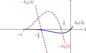
Figure 1: Functions appearing in the eigenvalue equation of $-ik\mathbf{L}_{1}+\mathbf{L}_{2}$; solid blue curve: $h_{0}(\lambda)$; red dash-dotted curve: $-h_{2}(\lambda)$; purple dashed line: $-h_{4}(\lambda)$. (colors only online)

This proves that the 5 velocity model is hypocoercive, at least in the norm $E$ defined in (4.8) (with the transformation matrices $\mathbf{P}_{k}$ now corresponding to $-\mathbf{C}_{k}:=\mp ik\mathbf{L}_{1}+\mathbf{L}_{2}$). The sharp decay rate is given by $\lambda_{0}=-0.526948302245121...$ .

To establish a uniform-in-$k$ spectral gap was already cumbersome for the case $n=4$, and it becomes even more involved for larger $n$. In the following section we present a much simpler strategy, at the price of giving up sharpness of the decay rate. But more importantly, that strategy will also be applicable for the continuous velocity case, which is represented by a tridiagonal “infinite matrix”.

4.3 A continuous velocity BGK model

In this subsection we continue our discussion of the space-inhomogeneous BGK equation (1.3) or, equivalently, (4.2). This will yield the proof of Theorem 1.1.

Using the probabilists’ Hermite polynomials,

$$H_{m}(v):=(-1)^{m}e^{\frac{v^{2}}{2}}\frac{{\rm d}^{m}}{{\rm d}v^{m}}e^{-\frac{v^{2}}{2}}\,,\quad m\in\mathbb{N}_{0}\,,$$ (4.14)

we define the normalized Hermite functions

$$g_{m}(v):=(2\pi m!)^{-1/2}H_{m}(v)\,e^{-\frac{v^{2}}{2}},\quad\mbox{and}\quad\tilde{g}_{m}(v):=\frac{1}{\sqrt{T}}g_{m}\big{(}\frac{v}{\sqrt{T}}\big{)}\,.$$ (4.15)

They satisfy

$$\int_{\mathbb{R}}\tilde{g}_{m}(v)\tilde{g}_{n}(v)M_{T}^{-1}(v)\,{\rm d}v=\delta_{mn}\,$$

and the recurrence relation

$$v\,\tilde{g}_{m}(v)=\sqrt{T}\big{[}\sqrt{m+1}\,\tilde{g}_{m+1}(v)+\sqrt{m}\,\tilde{g}_{m-1}(v)\big{]}\,.$$ (4.16)

In the basis $\{\tilde{g}_{m}\}_{m\in\mathbb{N}_{0}}$ Equation (4.2) becomes

$$\partial_{t}\hat{\bf f}_{k}+ik\sqrt{T}\,\mathbf{L}_{1}\hat{\bf f}_{k}=\mathbf{L}_{2}\hat{\bf f}_{k}\,,\quad t\geq 0;\;k\in\mathbb{Z}\,.$$ (4.17)

Here, the “infinite vector” $\hat{\bf f}_{k}(t)\in l^{2}(\mathbb{N}_{0})$ is the representation of the function $f_{k}(v,t)\in L^{2}(\mathbb{R};M_{T}^{-1})$ in the Hermite function basis, and the operators $\mathbf{L}_{1},\,\mathbf{L}_{2}$ are represented by “infinite matrices” as

$$\mathbf{L}_{1}=\left(\begin{array}[]{cccc}0&\sqrt{1}&0&\cdots\\ \sqrt{1}&0&\sqrt{2}&0\\ 0&\sqrt{2}&0&\sqrt{3}\\ \vdots&0&\sqrt{3}&\ddots\end{array}\right)\,,\quad\mathbf{L}_{2}=\operatorname{diag}(0,\,-1,\,-1,\,\cdots)\,.$$ (4.18)

Next we shall prove the exponential decay of (4.17), using a modified strategy compared to §4.2. For the 5 velocity model there, it was possible (with some effort) to determine the sharp spectral gap of the matrices $-ik\mathbf{L}_{1}+\mathbf{L}_{2}$, uniform in all modes $k$. But since this seems not (easily) possible for the infinite dimensional case in (4.17), we shall construct now approximate transformation matrices $\mathbf{P}_{k}$ that yield at least a (reasonable) lower bound on the spectral gap, and hence on the decay rate. For simplicity we set now $T=1$, as the temperature could be “absorbed” into the parameter $k$ by scaling.

Let $\mathbf{A}$ be an $(n+1)\times(n+1)$ tridiagonal matrix that is zero on the main diagonal. That is $A_{i,j}=0$ unless $j=i+1$ or $i=j-1$. We further suppose that $\mathbf{A}$ is real and symmetric, so that $\mathbf{A}$ is characterized by the numbers $a_{1},\dots,a_{n}$ where $a_{j}=A_{j-1,j}$. Let $\mathbf{B}={\rm diag}(0,-1,\dots,-1)$. Finally, for $k\in\mathbb{Z}$, consider the matrix $-\mathbf{C}_{k}:=-ik\mathbf{A}+\mathbf{B}$.

In the simplest case $n=1$ with $a=1$, we obtain

$$\mathbf{A}=\left(\begin{array}[]{cc}0&1\\ 1&0\end{array}\right)\,,\qquad\mathbf{B}=\left(\begin{array}[]{cc}0&\phantom{-}0\\ 0&-1\end{array}\right)\quad{\rm and}\quad-\mathbf{C}_{k}=\left(\begin{array}[]{cc}\phantom{-}0&-ik\\ -ik&-1\end{array}\right)\ .$$

For this matrix $\mathbf{C}_{k}$, the transformation matrix $\mathbf{P}_{k}$ was already computed in (4.5) (with $\sigma=1$). For $k\neq 0$ a simple computation yields

$$\mathbf{C}^{*}_{k}\mathbf{P}_{k}+\mathbf{P}_{k}\mathbf{C}_{k}=\mathbf{P}_{k}$$

so that with this choice of $\mathbf{P}_{k}$, Lyapunov’s method yields exponential decay of the ODE-sequence $\frac{\,\operatorname{d}\!}{\,\operatorname{d}\!t}u_{k}=-\mathbf{C}_{k}u_{k},\,k\in\mathbb{Z}$ at the optimal rate $e^{-t/2}$ (cf. §4.1).

We now turn to $n>1$. For $k\neq 0$ define $\mathbf{P}_{k}$ to be the $(n+1)\times(n+1)$ matrix whose upper left $2\times 2$ block is $\left(\begin{array}[]{cc}1&-i\alpha/k\\ i\alpha/k&1\end{array}\right)$, where $0<\alpha<k$ is a parameter to be chosen below, and with the remaining diagonal entries being $1$, and all other entries being $0$. Then the eigenvalues of $\mathbf{P}_{k}$ are $(k+\alpha)/k$, $1$ and $(k-\alpha)/k$, so that $\mathbf{P}_{k}$ is positive definite, and close to the identity for large $k$.

We take $-\mathbf{C}_{k}:=-ik\mathbf{A}+\mathbf{B}$ as above. Then

$$\mathbf{C}_{k}^{*}\mathbf{P}_{k}+\mathbf{P}_{k}\mathbf{C}_{k}=-ik(\mathbf{A}\mathbf{P}_{k}-\mathbf{P}_{k}\mathbf{A})-(\mathbf{B}\mathbf{P}_{k}+\mathbf{P}_{k}\mathbf{B})\ ,$$

and its upper left $3\times 3$ block reads

$$\left(\begin{array}[]{ccc}2a_{1}\alpha&-i\alpha/k&a_{2}\alpha\\ i\alpha/k&2-2a_{1}\alpha&0\\ a_{2}\alpha&0&2\end{array}\right)\ .$$ (4.19)

The lower right $(n-2)\times(n-2)$ block is $2$ times the identity, the off diagonal blocks are zero. In all of our finite dimensional approximations to (4.18) we have $a_{1}=1$. The value of $a_{2}$ is different for the different discrete velocity models, but to simplify matters, we only present calculations for $a_{2}=\sqrt{2}$, which is the value for the limiting continuous velocity model.

The determinants of the upper left $2\times 2$ and $3\times 3$ blocks read, respectively,

$$\delta_{2}(\alpha,k)=\alpha\left(4-\left(4+\frac{1}{k^{2}}\right)\alpha\right)\quad{\rm and}\quad\delta_{3}(\alpha,k)=4\alpha\left((\alpha-2)(\alpha-1)-\frac{\alpha}{2k^{2}}\right)\ .$$

For each $k$, $\delta_{3}(\alpha,k)/\alpha$ has two positive roots, and is negative between them. Hence our matrix is positive definite when $\alpha$ lies between zero and the smaller positive root of $\delta_{3}(\alpha,k)/\alpha$. This root is least when $k=1$, when it has the value $\frac{7-\sqrt{17}}{4}\approx 0.719$. Hence, by Sylvester’s criterion, $\mathbf{C}_{k}^{*}\mathbf{P}_{k}+\mathbf{P}_{k}\mathbf{C}_{k}$ is positive definite for all $k\neq 0$ if and only if $\alpha\in(0,\frac{7-\sqrt{17}}{4})\approx(0,0.719)$. Note that also $\delta_{2}(\alpha,k)>0$ for these $\alpha,k$.

When $\alpha$ is in this range, our $3\times 3$ matrix (4.19) has three positive eigenvalues $\lambda_{1}$, $\lambda_{2}$, $\lambda_{3}$ which we may take to be arranged in increasing order. Then

$$\sqrt{\lambda_{1}}=\frac{\sqrt{\delta_{3}(\alpha,k)}}{\sqrt{\lambda_{2}\lambda_{3}}}\geq\frac{2\sqrt{\delta_{3}(\alpha,k)}}{\lambda_{2}+\lambda_{3}}>\frac{\sqrt{\delta_{3}(\alpha,k)}}{2}$$

since the trace of our matrix is $4$. Hence, the least eigenvalue $\lambda_{1}$ of our $3\times 3$ matrix satisfies

$$\lambda_{1}=\lambda_{1}(\alpha,k)\geq\frac{1}{4}\delta_{3}(\alpha,k)\ .$$

Hence we choose $\alpha=\alpha_{k}$ to maximize $\delta_{3}(\alpha,k)$ between its first two roots. Its maximal value, $\delta_{3}(\alpha_{k},k)$, depends on $k$, but it is easily seen to be least for $k=1$ with $\alpha_{1}=\tfrac{1}{3}$. Simple computations and estimates then yield $\lambda_{1}(\alpha_{k},k)\geq\tfrac{1}{4}\delta_{3}(\alpha_{1},1)=17/54$ for all $k$.

Since we always take $\alpha<1$, the largest eigenvalue of the matrix ${\bf P}_{k}$ (defined with $\alpha=\alpha_{k}$) is no more than $2$, uniformly in $k$. Hence

$$\mathbf{C}_{k}^{*}\mathbf{P}_{k}+\mathbf{P}_{k}\mathbf{C}_{k}\geq\frac{17}{54}\mathbf{I}\geq\frac{17}{108}\mathbf{P}_{k}$$ (4.20)

uniformly in $k$. Thus in each Fourier mode, we at least have exponential decay (of a quadratic type entropy) at the rate $17/108$ (by proceeding as in (4.6)).

Since this is also uniform in $n$, we obtain a bound for the continuous velocity model. Let the infinite matrix ${\bf P}_{k}$ be the positive matrix using the optimal value of $\alpha$ in the $k$th mode, and regarded as a bounded operator on $L^{2}(M_{T}^{-1})$ through its action on Hermite modes. Define the entropy function by

$$e(f):=\sum_{k\in\mathbb{Z}}\big{\langle}(f_{k}(v)-M_{1}(v)),{\bf P}_{k}(f_{k}(v)-M_{1}(v))\big{\rangle}_{L^{2}(M_{1}^{-1})}\ .$$ (4.21)

We obtain that, for solutions $f(t)$ of our BGK equation (1.3) or, equivalently, (4.2),

$$\frac{{\rm d}}{{\rm d}t}e(f(t))\leq-\frac{17}{108}e(f(t))\ ,$$

giving exponential relaxation.

The least eigenvalue of $\mathbf{P}_{k}$, $1-\alpha/k$, is at least $1-\frac{7-\sqrt{17}}{4}>\frac{1}{4}$ uniformly in $k$, and hence we have the inequality

$$e(f)\geq\frac{1}{4}\|f-M_{1}\|^{2}_{\mathcal{H}}\ ,$$

with $\mathcal{H}=L^{2}(\mathbf{T}^{1}\times\mathbb{R};M_{T}^{-1}(v)\,\operatorname{d}\!v)$.

The above method to establish exponential decay is simple to apply but does not give the sharp decay rate (it is off by a factor of about 9, as indicated by numerical results). Hence we shall now sketch how to improve on it. The essence of the above method is to use an ansatz for the transformation matrix $\mathbf{P}_{k}$, namely to use for its upper left $2\times 2$ block the matrix from the 2 velocity case. Using instead larger blocks, will most likely improve the decay rate.

As a second alternative we shall now present an improvement of the crucial matrix inequality (4.20), but we shall keep the same ansatz for the matrix $\mathbf{P}_{k}$: In the inequality

$$\mathbf{C}_{k}^{*}\mathbf{P}_{k}+\mathbf{P}_{k}\mathbf{C}_{k}-2\mu\mathbf{P}_{k}\geq{\bf 0}$$ (4.22)

we shall choose $\mu\in[0,1]$ as large as possible (related to the matrix inequality (3.6)). The upper left $3\times 3$ block of this matrix on the l.h.s. reads

$$\mathbf{D}:=\left(\begin{array}[]{ccc}2\alpha-2\mu&-i\alpha(1-2\mu)/k&\sqrt{2}\alpha\\ i\alpha(1-2\mu)/k&2-2\alpha-2\mu&0\\ \sqrt{2}\alpha&0&2-2\mu\end{array}\right)\ .$$

We shall first derive strict inequalities on $\mu$ to obtain the positive definiteness of this matrix, using Sylvester’s criterion. From $\mathbf{D}_{0,0}$ we deduce the first condition $0\leq\mu<\alpha$. The determinant of the upper left $2\times 2$ block reads

$$\delta_{2}(\mu;\alpha,k)=4(\alpha-\mu)(1-\alpha-\mu)-\frac{\alpha^{2}}{k^{2}}(1-2\mu)^{2}\,.$$

Since the last term increases with $|k|$, it suffices to consider $\delta_{2}$ for $k=1$. Next we want to establish the positivity of

$$\frac{\delta_{2}(\mu;\alpha,1)}{4(1-\alpha^{2})}=\mu^{2}-\mu+\alpha\frac{1-5\alpha/4}{1-\alpha^{2}}\,.$$

The zero order term of this quadratic polynomial is positive on the relevant $\alpha$–interval $(0,\frac{7-\sqrt{17}}{4})\subset(0,\frac{4}{5})$, taking its maximum value $\frac{1}{4}$ at $\alpha=\frac{1}{2}$. For that limiting case, the r.h.s. reads $(\mu-\frac{1}{2})^{2}$, and for $0<\alpha<\frac{1}{2}$, $\delta_{2}(\mu;\alpha,1)$ always has a zero in the interval $(0,\frac{1}{2})$. This discussion yields the second condition $0\leq\mu<\frac{1}{2}$, related to $\alpha<\frac{1}{2}$.

Next we consider the positivity of the determinant of the upper left $3\times 3$ block, which reads

$$\delta_{3}(\mu;\alpha,k)=8(1-\mu)(\alpha-\mu)(1-\alpha-\mu)-4\alpha^{2}(1-\alpha-\mu)-2\frac{\alpha^{2}}{k^{2}}(1-\mu)(1-2\mu)^{2}\,.$$

For the same reason as before, we only have to consider the case $k=1$. For the resulting cubic polynomial in $\mu$ we want to find its largest zero in the interval $[0,\frac{1}{2}]$ w.r.t. the parameter $\alpha\in[0,\frac{1}{2}]$. By numerical inspection we find that $\alpha_{0}\approx 0.4684$ yields $\delta_{3}(\mu;\alpha_{0},1)\geq 0$ for $\mu\in[0,0.273796...]$. This yields the third condition on $\mu$ and shows that the matrix inequality (4.22) holds with $\mu_{0}:=0.273796...$, uniformly in $k\neq 0$. This somewhat more involved discussion shows that the decay rate can be improved to $2\mu_{0}\approx 0.547592$. This finishes the proof of Theorem 1.1.

Remark: To appreciate the above decay rate $\mu_{0}$ (since $e(f)$ is a quadratic functional), we compare it to a numerical computation of the spectral gap of the “infinite matrices” $-ik\mathbf{L}_{1}+\mathbf{L}_{2},\,k\in\mathbb{Z}$ from (4.18). To this end we cut out the upper left $n\times n$ submatrix for large values of $n$. For increasing $n$ the spectral gap approaches $0.6973$. Hence our decay rate is off by only a factor of about $2.5$. If one desired a closer bound, one could work with a $\mathbf{P}$ matrix with a larger block, say $3\times 3$, in the upper left.

4.4 Linearized BGK equation

Next we shall analyze here the linearized BGK equation (1.12) for the perturbation $h(x,v,t)=f(x,v,t)-M_{T}(v)$. We recall the definition of the normalized Hermite functions $\tilde{g}_{m}(v)$, $m\in\mathbb{N}_{0}$ from (4.15) and give explicit expressions for

$$\tilde{g}_{0}(v)=M_{T}(v)\quad{\rm and}\quad\tilde{g}_{2}(v)=\frac{v^{2}-T}{\sqrt{2}T}\ M_{T}(v)\ .$$

With this notation, (1.12) reads

$$h_{t}(x,v,t)+vh_{x}(x,v,t)=\left(\tilde{g}_{0}(v)-\frac{1}{\sqrt{2}}\tilde{g}_{2}(v)\right)\sigma(x,t)+\frac{1}{\sqrt{2}T}\tilde{g}_{2}(v)\tau(x,t)-h(x,v,t)\ .$$

Fourier transforming in $x$, as in (4.1), each spatial mode $h_{k}(v,t)$ evolves as

$$\partial_{t}h_{k}+ikvh_{k}=\tilde{g}_{0}(v)\sigma_{k}(t)+\tilde{g}_{2}(v)\frac{1}{\sqrt{2}}\left(\frac{\tau_{k}(t)}{T}-\sigma_{k}(t)\right)-h_{k}\,,\quad k\in\mathbb{Z};\,t\geq 0\ .$$ (4.23)

Here, $\sigma_{k}$ and $\tau_{k}$ denote the spatial modes of the $v$–moments $\sigma$ and $\tau$ defined in (1.8).

Next we expand $h_{k}(\cdot,t)\in L^{2}(\mathbb{R};M_{T}^{-1})$ in the orthonormal basis $\{\tilde{g}_{m}(v)\}_{m\in\mathbb{N}_{0}}$:

$$h_{k}(v,t)=\sum_{m=0}^{\infty}\hat{h}_{k,m}(t)\,\tilde{g}_{m}(v)\,,\quad\mbox{with }\quad\hat{h}_{k,m}=\langle h_{k}(v),\tilde{g}_{m}(v)\rangle_{L^{2}(M_{T}^{-1})}\ ,$$

and the “infinite vector” $\hat{\bf h}_{k}(t)=(\hat{h}_{k,0}(t),\,\hat{h}_{k,1}(t),\,...)^{\top}\in\ell^{2}(\mathbb{N}_{0})$ contains all Hermite coefficients of $h_{k}(\cdot,t)$, for each $k\in\mathbb{Z}$. In particular we have

$$\hat{h}_{k,0}=\int_{\mathbb{R}}h_{k}(v)\tilde{g}_{0}(v)M_{T}^{-1}(v)\,\operatorname{d}\!v=\sigma_{k}$$

and

$$\hat{h}_{k,2}=\int_{\mathbb{R}}h_{k}(v)\tilde{g}_{2}(v)M_{T}^{-1}(v)\,\operatorname{d}\!v=\frac{1}{\sqrt{2}}\left(\frac{\tau_{k}}{T}-\sigma_{k}\right)\ .$$

Hence, (4.23) can be written equivalently as

$$\partial_{t}h_{k}(v,t)+ikvh_{k}(v,t)=\tilde{g}_{0}(v)\hat{h}_{k,0}(t)+\tilde{g}_{2}(v)\hat{h}_{k,2}(t)-h_{k}(v,t)\,,\quad k\in\mathbb{Z};\,t\geq 0\ .$$

In analogy to (4.17), its Hermite coefficients satisfy

$$\partial_{t}\hat{\bf h}_{k}(t)+ik\sqrt{T}\,\mathbf{L}_{1}\hat{\bf h}_{k}(t)=\mathbf{L}_{3}\hat{\bf h}_{k}(t)\,,\quad k\in\mathbb{Z};\,t\geq 0\ ,$$ (4.24)

where the operators $\mathbf{L}_{1},\,\mathbf{L}_{3}$ are represented by “infinite matrices” on $\ell^{2}(\mathbb{N}_{0})$ by

$$\mathbf{L}_{1}=\left(\begin{array}[]{cccc}0&\sqrt{1}&0&\cdots\\ \sqrt{1}&0&\sqrt{2}&0\\ 0&\sqrt{2}&0&\sqrt{3}\\ \vdots&0&\sqrt{3}&\ddots\end{array}\right)\,,\quad\mathbf{L}_{3}=\operatorname{diag}(0,\,-1,\,0,\,-1,\,-1,\cdots)\,.$$

We remark that (4.24) simplifies for the spatial mode $k=0$. One easily verifies that the flow of (1.12) preserves (1.9), i.e. $\sigma_{0}(t)=0$, $\tau_{0}(t)=0$ $\forall t\geq 0$. Hence, (4.23) yields

$$\partial_{t}h_{0}(v,t)=-h_{0}(v,t)\,,\quad t\geq 0\ .$$

For $k\neq 0$, we note that the linearized BGK equation is very similar to the equation specified in (4.17) and (4.18): The only difference is that $\mathbf{L}_{2}$ is replaced by $\mathbf{L}_{3}$, which has one more zero on the diagonal. Our treatment of $ik\sqrt{T}\mathbf{L}_{1}-\mathbf{L}_{2}$ in the previous section suggests the form of the positive matrix $\mathbf{P}_{k}$ that will provide our Lyapunov functional in this case. We obtained the matrix $\mathbf{P}_{k}$ in that case by replacing four entries around the location of the zero in $\mathbf{L}_{2}$ with the entries of $\left(\begin{array}[]{cc}1&-i\alpha/k\\ i\alpha/k&1\end{array}\right)$, the matrix that provides the optimal $\mathbf{P}_{k}$ for the two-velocity model. In the present case, we use two such matrices, one for each zero.

For parameters $\alpha$ and $\beta$ to be chosen below, we define $\mathbf{P}_{k}$ to be the matrix that has

$$\left(\begin{array}[]{cccc}1&-i\alpha/k&0&0\\ i\alpha/k&1&0&0\\ 0&0&1&-i\beta/2k\\ 0&0&i\beta/2k&1\end{array}\right)\$$ (4.25)

as its upper-left $4\times 4$ block, with all other entries being those of the identity. We define $-\mathbf{C}_{k}=-ik\mathbf{L}_{1}+\mathbf{L}_{3}$, where, for the rest of this subsection, we use units in which $T=1$.

Lemma 4

Choosing $\alpha=\beta=1/3$ in $\mathbf{P}_{k}$ uniformly in $|k|\in\mathbb{N}$, we have

$$\mathbf{C}_{k}^{*}\mathbf{P}_{k}+\mathbf{P}_{k}\mathbf{C}_{k}\geq 2\mu\mathbf{P}_{k}$$ (4.26)

where

$$\mu=0.0206\ .$$ (4.27)

Proof

We compute that $\mathbf{C}_{k}^{*}\mathbf{P}_{k}+\mathbf{P}_{k}\mathbf{C}_{k}$ is twice the identity matrix whose upper left $5\times 5$ block is replaced by

$$\mathbf{D}_{k,\alpha,\beta}=\left(\begin{array}[]{ccccc}2\alpha&-i\alpha/k&\sqrt{2}\alpha&0&0\\ i\alpha/k&2-2\alpha&0&-\beta/\sqrt{2}&0\\ \sqrt{2}\alpha&0&\sqrt{3}\beta&-i\beta/2k&\beta\\ 0&-\beta/\sqrt{2}&i\beta/2k&2-\sqrt{3}\beta&0\\ 0&0&\beta&0&2\end{array}\right)\,.$$

We seek to choose $\alpha$ and $\beta$ to make this matrix positive definite.

For $1\leq j\leq 5$, let $\delta_{j}(k,\alpha,\beta)$ denote the determinant of the upper left $j\times j$ submatrix of $\mathbf{D}_{k,\alpha,\beta}$. For $\alpha=\beta$, the first and third column of $\mathbf{D}_{k,\alpha,\beta}$ have the common factor $\alpha$. We then compute that

$$\delta_{5}(k,\alpha,\alpha)=\alpha^{2}p_{5}(\alpha,k)\,,$$

where $p_{5}(\alpha,k)$ is a cubic polynomial in $\alpha$ with coefficients depending on $k$:

$$p_{5}(\alpha,k) =16(\sqrt{3}-1)-\left[8\sqrt{3}+16+\frac{2+4\sqrt{3}}{k^{2}}\right]\alpha$$

$$\quad+\left[34-6\sqrt{3}+\frac{24k^{2}+1}{2k^{4}}\right]\alpha^{2}-\left[4\sqrt{3}-1+\frac{\sqrt{3}}{k^{2}}\right]\alpha^{3}\,.$$

Next, we establish the bound

$$p_{5}(\alpha,k)\geq p_{5}(\alpha,1)\\ =16(\sqrt{3}-1)-(12\sqrt{3}+18)\alpha+(46.5-6\sqrt{3})\alpha^{2}-(5\sqrt{3}-1)\alpha^{3}>0$$ (4.28)

for $\alpha\in[0,\alpha_{1}]$ with $\alpha_{1}\approx 0.555$ and $|k|\in\mathbb{N}$. To see the first inequality we consider

$$p_{5}(\alpha,k)-p_{5}(\alpha,1)=\alpha(1-\tfrac{1}{k^{2}})\varphi(\alpha,k)$$

with

$$\varphi(\alpha,k):=\sqrt{3}\alpha^{2}-\big{(}\tfrac{1}{2}(1+\tfrac{1}{k^{2}})+12\big{)}\alpha+2+4\sqrt{3}.$$

It satisfies $\varphi(\alpha,1)>0$ for $\alpha\in[0,\alpha_{2}]$ with $\alpha_{2}\approx 0.765$ and $\partial_{k}\varphi=\alpha/k^{3}$ for $\alpha\geq 0$ and $k\in\mathbb{N}$. The r.h.s. of (4.28) is easily seen to be monotone decreasing and evaluating it at $\alpha=1/3$ and simplifying, we obtain $p_{5}(\alpha,k)\geq 2.5$ for $\alpha\in[0,1/3]$. Finally, we then have

$$\delta_{5}(k,\alpha,\alpha)\geq 2.5\alpha^{2}$$

for $\alpha\in[0,1/3]$ and all $k\neq 0$. A similar but simpler analysis shows that for $j=1,2,3,4$, $\delta_{j}(k,\alpha,\alpha)>0$ for $\alpha\in[0,1/3]$ and all $k\neq 0$.

Thus, we choose $\alpha=\beta=1/3$ uniformly in $k$ and this makes $\mathbf{D}_{k,\alpha,\beta}$ positive definite. Let $\{\lambda_{1},\lambda_{2},\lambda_{3},\lambda_{4},\lambda_{5}\}$ be the eigenvalues of $\mathbf{D}_{k,1/3,1/3}$ arranged in increasing order. We seek a lower bound on $\lambda_{1}$. Note that by the arithmetic-geometric mean inequality,

$$\lambda_{1}=\frac{\delta_{5}(k,1/3,1/3)}{\lambda_{2}\lambda_{3}\lambda_{4}\lambda_{5}} \geq \delta_{5}(k,1/3,1/3)\left(\frac{\lambda_{2}+\lambda_{3}+\lambda_{4}+\lambda_{5}}{4}\right)^{-4}$$

$$\geq 256\ \frac{\delta_{5}(k,1/3,1/3)}{(\operatorname{Tr}[\mathbf{D}_{k,1/3,1/3}])^{4}}\ .$$

Since $\operatorname{Tr}[\mathbf{D}_{k,\alpha,\beta}]=6$ independent of $k$, $\alpha$ and $\beta$, we finally obtain the bound $\lambda_{1}\geq 0.0549$, and this means that, uniformly in $k\neq 0$,

$$\mathbf{C}_{k}^{*}\mathbf{P}_{k}+\mathbf{P}_{k}\mathbf{C}_{k}\geq 0.0549\ {\bf I}\ .$$ (4.29)

A simple computation shows that the eigenvalues of $\mathbf{P}_{k}$ are $1$, $1\pm 1/6k$, and $1\pm 1/3k$. Hence uniformly in $k$,

$$\frac{2}{3}{\bf I}\leq\mathbf{P}_{k}\leq\frac{4}{3}{\bf I}\ .$$ (4.30)

Combining (4.30) with (4.29) yields the result. ∎∎

To deduce the first statement of Theorem 1.2 we consider a solution $h$ of (1.12), and for $\gamma\geq 0$ the entropy functional $e_{\gamma}(f)$ defined by

$$e_{\gamma}(f):=\sum_{k\in\mathbb{Z}}(1+k^{2})^{\gamma}\langle h_{k}(v),\mathbf{P}_{k}h_{k}(v)\rangle_{L^{2}(M_{T}^{-1})}\ ,$$ (4.31)

with $f=M_{1}+h$. Here the matrices $\mathbf{P}_{0}=\mathbf{I}$ and $\mathbf{P}_{k}$ defined in (4.25) for $k\neq 0$ are regarded as bounded operators on $L^{2}(M_{T}^{-1})$. Then

$$\frac{\,\operatorname{d}\!}{\,\operatorname{d}\!t}e_{\gamma}(f)=-\sum_{k\in\mathbb{Z}}(1+k^{2})^{\gamma}\langle h_{k}(v),(\mathbf{C}_{k}^{*}\mathbf{P}_{k}+\mathbf{P}_{k}\mathbf{C}_{k})h_{k}(v)\rangle_{L^{2}(M_{T}^{-1})}\leq-0.0412\,e_{\gamma}(f)\ ,$$ (4.32)

which implies (1.14) and this finishes the proof of Theorem 1.2(a).

We note that the constant in (4.32) is within a factor of 18 of what numerical calculation shows is best possible. With more work, in particular not making the simplifying assumption $\alpha=\beta$ in the definition of $\mathbf{P}$, and also employing some of the ideas in the final part of section 4.3, one can still better within this framework.

4.5 Local asymptotic stability for the BGK equation

For $\gamma\geq 0$, let $H^{\gamma}(\mathbf{T}^{1})$ be the Sobolev space consisting of the completion of smooth functions $\varphi$ on $\mathbf{T}^{1}$ in the Hilbertian norm

$$\|\varphi\|_{H^{\gamma}}^{2}:=\sum_{k\in\mathbb{Z}}(1+k^{2})^{\gamma}|\varphi_{k}|^{2}\ ,$$

where $\varphi_{k}$ is the $k$th Fourier coefficient of $\varphi$. Let $\mathcal{H}_{\gamma}$ denote the Hilbert space $H^{\gamma}(\mathbf{T}^{1})\otimes L^{2}(\mathbb{R};M_{T}^{-1}(v)\,\operatorname{d}\!v)$, where the inner product in $\mathcal{H}_{\gamma}$ is given by

$$\langle f,g\rangle_{\mathcal{H}_{\gamma}}=\int_{\mathbf{T}^{1}}\int_{\mathbb{R}}\overline{f}(x,v)\left[\left(1-\partial_{x}^{2}\right)^{\gamma}g(x,v)\right]M_{T}^{-1}(v){\rm d}v{\rm d}\tilde{x}\ ,$$

where $\,\operatorname{d}\!\tilde{x}$ denotes the normalized Lebesgue measure on $\mathbf{T}^{1}$.

Then $\mathcal{H}_{0}$ is simply the weighted space $L^{2}(\mathbf{T}^{1}\times\mathbb{R};M_{T}^{-1}(v)\,\operatorname{d}\!v)$ and, for all $\gamma\geq 0$, ${\bf Q}$ is self-adjoint on $\mathcal{H}_{\gamma}$.

Let $\rho$, $P$, $\sigma$ and $\tau$ be defined in terms of a density $f$ as in (1.8). For all $\gamma$, $\|\sigma\|_{H^{\gamma}}^{2}=\langle\sigma M_{T},f-f^{\infty}\rangle_{\mathcal{H}_{\gamma}}$. Then by the Cauchy-Schwarz inequality,

$$\|\sigma\|_{H^{\gamma}}^{2}\leq\|\sigma M_{T}\|_{\mathcal{H}_{\gamma}}\|f-f^{\infty}\|_{\mathcal{H}_{\gamma}}=\|\sigma\|_{H^{\gamma}}\|f-f^{\infty}\|_{\mathcal{H}_{\gamma}}\ .$$ (4.33)

Likewise, $\|\tau\|_{H^{\gamma}}^{2}=\langle\tau v^{2}M_{T},f-f^{\infty}\rangle_{\mathcal{H}_{\gamma}}$, and by the Cauchy-Schwarz inequality,

$$\|\tau\|_{H^{\gamma}}^{2}\leq\|\tau v^{2}M_{T}\|_{\mathcal{H}_{\gamma}}\|f-f^{\infty}\|_{\mathcal{H}_{\gamma}}=\sqrt{3}T\|\tau\|_{H^{\gamma}}\|f-f^{\infty}\|_{\mathcal{H}_{\gamma}}\ .$$ (4.34)

For $\gamma>1/2$, functions in $H^{\gamma}$ are Hölder continuous, and the $H^{\gamma}$ norm controls their supremum norm. Combining this with the estimates proved above, we see that for all $\gamma>1/2$, there is a finite constant $C_{\gamma}$ such that the pressure and density satisfy

$$\|\sigma\|_{\infty}=\|\rho-1\|_{\infty}\leq C_{\gamma}\|f-f^{\infty}\|_{\mathcal{H}_{\gamma}}\qquad{\rm and}\qquad\|\tau\|_{\infty}=\|P-T\|_{\infty}\leq C_{\gamma}\|f-f^{\infty}\|_{\mathcal{H}_{\gamma}}\ .$$ (4.35)

Using these estimates it is a simple matter to control the approximation in (1.10). For $s\in[0,1]$ and $(x,v)\in\mathbf{T}^{1}\times\mathbb{R}$, define

$$F(s,x,v):=\frac{(1+s\sigma(x))^{3/2}}{\sqrt{2\pi(T+s\tau(x))}}e^{-v^{2}(1+s\sigma(x))/2(T+s\tau(x))}\ ,$$

so that the gain term in the linearized BGK equation (1.12) is ${\displaystyle\partial_{s}F(0,x,v)}$. In this notation,

$$R_{f}(x,v):=$$

$$\qquad M_{f}(x,v)-M_{T}(v)-\left[\left(\frac{3}{2}-\frac{v^{2}}{2T}\right)M_{T}(v)\sigma(x)+\left(-\frac{1}{2T}+\frac{v^{2}}{2T^{2}}\right)M_{T}(v)\tau(x)\right]$$

$$\qquad=\int_{0}^{1}\left[\partial_{s}F(s,x,v)-\partial_{s}F(0,x,v)\right]{\rm d}s=\int_{0}^{1}\int_{0}^{s}\left[\partial_{s}^{2}F(r,x,v)\right]{\rm d}r{\rm d}s\ .$$

We compute

$$\partial_{s}^{2}F(s,x,v)$$ (4.36)

$$=\frac{\tau-T\sigma}{(1+s\sigma)^{2}}\left[-\frac{3\sigma}{4\theta_{s}}+\bigg{(}\frac{3}{2}v^{2}\sigma+\frac{3}{4}\tau\bigg{)}\frac{1}{\theta_{s}^{2}}-\bigg{(}\frac{1}{4}v^{4}\sigma+\frac{3}{2}v^{2}\tau\bigg{)}\frac{1}{\theta_{s}^{3}}+\frac{v^{4}\tau}{4\theta_{s}^{4}}\right]M_{\theta_{s}}(v)$$

with the notations $\theta_{s}:=\frac{T+s\tau}{1+s\sigma}$ and $M_{\theta_{s}}(v):=\frac{1}{\sqrt{2\pi\theta_{s}}}e^{-v^{2}/(2\theta_{s})}$. Note that the r.h.s. of (4.36) is of the order $\mathcal{O}(\sigma^{2}+\tau^{2})$, which will be related to $\mathcal{O}((f-f^{\infty})^{2})$ due to the estimates (4.33)-(4.34).

Simple but cumbersome calculations now show that if $\gamma>1/2$ and $\|{f-f^{\infty}}\|_{\mathcal{H}_{\gamma}}$ is sufficiently small, then there exists a finite constant $\tilde{C}_{\gamma,T}$ depending only on $\gamma$ and $T$ such that for all $s\in[0,1]$,

$$\left\|\partial_{s}^{2}F(s,x,v)\right\|_{\mathcal{H}_{\gamma}}\leq\tilde{C}_{\gamma,T}\|f-f^{\infty}\|_{\mathcal{H}_{\gamma}}^{2}\ ,$$ (4.37)

and hence

$$\|R_{f}\|_{\mathcal{H}_{\gamma}}\leq\tilde{C}_{\gamma,T}\|f-f^{\infty}\|_{\mathcal{H}_{\gamma}}^{2}\ .$$ (4.38)

[The calculations are simplest for non-negative integer $\gamma$, in which case the Sobolev norms can be calculated by differentiation. For $\gamma>1/2$ and sufficiently small $\|{f-f^{\infty}}\|_{\mathcal{H}_{\gamma}}$, the estimates (4.35) ensure for all $s\in[0,1]$ the boundedness of $0<\epsilon<\|{1+s\sigma}\|_{\infty}\ ,\,\|{T+s\tau}\|_{\infty}<\infty$ for some fixed $\epsilon>0$ and the $L^{2}(\mathbb{R};M_{T}^{-1}(v)\,\operatorname{d}\!v)$-integrability of

$$e^{-v^{2}(1+s\sigma(x))/2(T+s\tau(x))}\leq e^{-v^{2}/3T}\quad\text{for all }x\ .$$

In (4.37), higher powers of $\|{f-f^{\infty}}\|_{\mathcal{H}_{\gamma}}$ (arising due to derivatives of $\sigma$ and $\tau$) can be absorbed into the constant of the quadratic term.]

Now let $f$ be a solution of the BGK equation (1.6) with constant temperature $T=1$ and define $h(x,v,t):=f(x,v,t)-M_{T}(v)$ as in the introduction. Now define the linearized BGK operator

$$\mathbf{Q}_{2}h(x,v,t):=\left(\frac{3}{2}-\frac{v^{2}}{2T}\right)M_{T}(v)\sigma(x)+\left(-\frac{1}{2T}+\frac{v^{2}}{2T^{2}}\right)M_{T}(v)\tau(x)-h(x,v,t)$$ (4.39)

where of course $\sigma$ and $\tau$ are determined by $f$, and hence $h$. Then the nonlinear BGK equation (1.6) becomes

$$h_{t}(x,v,t)+v\ h_{x}(x,v,t)=\mathbf{Q}_{2}h(x,v,t)+R_{f}(x,v,t)\ ,\qquad t\geq 0\ ,$$ (4.40)

which deviates from the linearized BGK equation (1.12) only by the additional term $R_{f}$.

It is now a simple matter to prove local asymptotic stability. We shall use here exactly the entropy functional $e_{\gamma}(f)$ defined in (4.31) with $f=M_{1}+h$. Now assume that $h$ solves (4.40). To compute $\frac{{\rm d}}{{\rm d}t}e_{\gamma}(f)$ we use the inequality (4.32) for the drift term and for $\mathbf{Q}_{2}h$ in (4.40), as well as $\|\mathbf{P}_{k}\|\leq\frac{4}{3}$ and (4.38) for the term $R_{f}$. This yields

$$\frac{{\rm d}}{{\rm d}t}e_{\gamma}(f)\leq-0.0412\,e_{\gamma}(f)+\frac{8}{3}\tilde{C}_{\gamma,T}\|h\|_{\mathcal{H}_{\gamma}}^{3}\ ,$$ (4.41)

(if $\|h\|_{\mathcal{H}_{\gamma}}$ is small enough) where we have used the fact that $h=f-f^{\infty}$. Then since

$$\frac{2}{3}e_{\gamma}(f)\leq\|h\|_{\mathcal{H}_{\gamma}}^{2}\leq\frac{4}{3}e_{\gamma}(f)\ ,$$

which is simply a restatement of (4.30), it is now simple to complete the proof of Theorem 1.2(b): Estimate (4.41) shows that there is a $\delta_{\gamma}>0$ so that if the initial data $f^{I}(x,v)$ satisfies $\|f^{I}-f^{\infty}\|_{\mathcal{H}_{\gamma}}<\delta_{\gamma}$, then the solution $f(t)$ satisfies

$$e_{\gamma}(f(t))\leq e^{-t/25}e_{\gamma}(f^{I})\ .$$

Here we used that the linear decay rate in (4.41) is slightly better than $\frac{1}{25}$, to compensate the nonlinear term.

We expect that the strategy from this section can be adapted also to nonlinear kinetic Fokker-Planck equations; this will be the topic of a subsequent work.

- (1) Achleitner, F., Arnold, A., Stürzer, D.: Large-time behavior in non-symmetric Fokker-Planck equations. to appear in Rivista di Matematica della Università di Parma (2015)
- (2) Arnold, A., Carlen, E., and Ju, Q.: Large-time behavior of non-symmetric Fokker-Planck type equations. Commun. Stoch. Anal. 2, no. 1, 153–175 (2008)
- (3) Arnold, A., and Erb, J. Sharp entropy decay for hypocoercive and non-symmetric Fokker-Planck equations with linear drift. arXiv preprint arXiv:1409.5425 (2014)
- (4) Arnold, A., Markowich, P., Toscani, G., and Unterreiter, A. On convex Sobolev inequalities and the rate of convergence to equilibrium for Fokker-Planck type equations. Comm. Partial Differential Equations 26, no. 1-2, 43–100 (2001)
- (5) Bakry, D., and Émery, M. Hypercontractivité de semi-groupes de diffusion. C. R. Acad. Sci. Paris Sér. I Math. 299, no. 15, 775–778 (1984)
- (6) Bakry, D., and Émery, M. Diffusions hypercontractives. In Séminaire de probabilités, XIX, 1983/84, vol. 1123 of Lecture Notes in Math. Springer, Berlin 177–206 (1985)
- (7) Bergmann, P., and Lebowitz, J.L. A new approach to nonequilibrium processes. Phys. Rev. 99, no. 2, 578–587 (1955)
- (8) Bhatnagar, P.L., Gross, E.P., and Krook, M. A Model for Collision Processes in Gases. I. Small Amplitude Processes in Charged and Neutral One-Component Systems. Physical Review 94, no. 3, 511–525 (1954)
- (9) Bobkov, S.G., and Tetali, P. Modified logarithmic Sobolev inequalities in discrete settings. J. Theoret. Probab. 19, no. 2, 289–336 (2006)
- (10) Bosi, R., and Cáceres, M. J., The BGK model with external confining potential: existence, long-time behaviour and time-periodic Maxwellian equilibria. J. Stat. Phys. 136, no. 2, 297–330 (2009)
- (11) Coleman, R. On Krawtchouk polynomials. arXiv preprint arXiv:1101.1798 (2011)
- (12) Diaconis, P., and Saloff-Coste, L. Logarithmic Sobolev inequalities for finite Markov chains. Ann. Appl. Probab. 6, no. 3, 695–750, (1996)
- (13) Dolbeault, J., Mouhot, C., and Schmeiser, C. Hypocoercivity for linear kinetic equations conserving mass. Trans. Amer. Math. Soc. 367, no. 6, 3807–3828 (2015)
- (14) Dolbeault, J., Mouhot, C., and Schmeiser, C. Hypocoercivity for kinetic equations with linear relaxation terms. C. R. Math. Acad. Sci. Paris 347, no. 9-10, 511–516 (2009)
- (15) Hérau, F., Hypocoercivity and exponential time decay for the linear inhomogeneous relaxation Boltzmann equation. Asymptot. Anal. 46, no. 3-4, 349–359 (2006)
- (16) Horn, R.A., and Johnson, C.R. Matrix analysis. Cambridge University Press, Cambridge, 2nd ed. (2013)
- (17) Horn, R.A., and Johnson, C.R. Topics in matrix analysis. Cambridge University Press, Cambridge, (1991)
- (18) Kac, M. Foundations of kinetic theory, Proc. 3rd Berkeley Symp. Math. Stat. Prob., J. Neyman, ed. Univ. of California, vol 3, 171–197 (1956)
- (19) Michel, A.N., Hou, L., and Liu, D. Stability of dynamical systems. Birkhäuser/Springer, 2nd ed. (2015)
- (20) Norris, J.R. Markov chains. Cambridge University Press, Cambridge, (1997)
- (21) Perthame, B. Global existence to the BGK model of Boltzmann equation. J. Differential Equations 82, no. 1, 191–205 (1989)
- (22) Perthame, B. Transport Equations in Biology. Birkhäuser, Basel (2007)
- (23) Perthame, B. and Pulvirenti, M. Weighted bounds and uniqueness for the Boltzmann BGK model. Arch. Rational Mech. Anal. 125, no. 3, 289–295 (1993)
- (24) Seneta, E. Nonnegative matrices and Markov chains. Springer Series in Statistics, 2nd ed., Springer-Verlag, New York, (1981)
- (25) van Kampen, N.G. Stochastic processes in physics and chemistry. Elsevier, 3rd ed. (2007)
- (26) Villani, C. Hypocoercivity. Mem. Amer. Math. Soc. 202, no. 950 (2009)