Non-LTE Equivalent Widths for N ii with Error Estimates

Abstract

Non-LTE calculations are performed for N ii in stellar atmospheric models appropriate to main sequence B-stars to produce new grids of equivalent widths for the strongest N ii lines commonly used for abundance analysis. There is reasonable agreement between our calculations and previous results, although we find weaker non-LTE effects in the strongest optical N ii transition, $\lambda\,3995$. We also present a detailed estimation of the uncertainties in the equivalent widths due to inaccuracies in the atomic data via Monte Carlo simulation and investigate the completeness of our model atom in terms of included energy levels. Uncertainties in the basic N ii atomic data limit the accuracy of abundance determinations to $\approx\,\pm 0.10\,$dex at the peak of the N ii optical spectrum near $T_{\rm eff}\approx 24,000\,$K.

1 Introduction

Accurate abundance measurements in the atmospheres of massive, upper main sequence stars represent an important test of current models of stellar evolution (Maeder & Meynet, 2012; Palacios, 2013). Accurate CNO abundances, and nitrogen abundances in particular, are of special significance due to their potential role as diagnostics of rotational mixing (e.g. Heger & Langer (2000), Heger et al. (2000), Meynet & Maeder (2000), Brott er al. (2011), Ekström et al. (2012), Granada & Haemmerlé (2014), Maeder et al. (2014)). Stellar rotation velocities reach their peak on the main sequence among the early-B and late-O-type stars (Fukuda, 1982), and rapid rotation is predicted to mix CNO-processed material into the stellar atmospheres, with the resulting nitrogen enhancement being the easiest to detect (Talon et al., 1997; Meynet & Maeder, 2000; Heger et al., 2000; Brott er al., 2011). Searches for enhanced nitrogen abundances among main sequence B stars have produced mixed results (Maeder et al., 2009; Hunter et al., 2009; Nieva & Przybilla, 2014), and surprisingly, no nitrogen enhancements have been found among the Be stars, which are the most rapidly-rotating population on the main sequence (Lennon et al., 2005; Dunstall et al., 2011).

Accurate abundance analysis for B stars is complicated by several factors: departures from local thermodynamic equilibrium (LTE), rapid rotation (which introduces several issues– see below), and, in cases such as the Be stars, potential emission from circumstellar material.

Departure from LTE is a well known problem in early-type and evolved stars (Mihalas, 1978; Kurucz, 1979). In the non-LTE case, the calculation must account for the non-local radiation field in the photosphere due to photons coming from hotter, deeper layers and from photon loss through the outer boundary. As a result, the level populations will differ from the Saha-Boltzmann predictions at the local electron temperature and density. To obtain the line source functions and optical depth scales required for the line transfer problem, the coupled equations of radiative transfer and statistical equilibrium must be solved in a self-consistent manner (Mihalas, 1978; Cannon, 1985).

The large broadening of spectral lines in early-type stars due to rapid rotation results in shallow and wide lines with low continuum contrast and, potentially, strong line blending. In such cases, only a few, strong, spectral lines of each element can be reliably measured. The use of only the strongest lines of a given element can compromise the accuracy of the abundance analysis due to (typically) stronger non-LTE effects, the confounding influence of microturbulence, and the dependence of the equivalent widths on uncertain damping parameters. In addition, the traditional method of estimating uncertainties from the dispersion of the measured elemental abundance from many measured weak and strong lines cannot be applied. In the case where only a few strong lines of a given element are available, a detailed theoretical error analysis is required to give the measured abundances meaning. This can be handled by Monte Carlo simulation of the errors introduced by uncertain atomic data (including damping widths), uncertain stellar parameters ($T_{\rm eff}$, $\log\,g$, and the microturbulence), and the uncertainty in the measured equivalent width (Sigut, 1996).

Complications due to rapid rotation include gravitational darkening, where the stellar surface distorts and the temperature and gravity become dependent on latitude (Von Zeipel, 1924). As a consequence, the strengths of spectral lines will be dependent on the stellar inclination (Stoeckley & Nuscombe, 1987). Finally, in the case of the Be stars, there is the possibility of contamination by circumstellar material (Porter & Rivinus, 2003).

In this paper, the focus is on the limiting accuracy of predicted N ii equivalent widths due to uncertainties in the basic atomic data used in the non-LTE calculation. The methodology follows that of Sigut (1996), and the structure of the paper is as follows: In Section (2), we give a brief summary of previous non-LTE calculations for N ii. In Section (3), we discuss the atomic data used to construct our nitrogen atom. In Section (4), the results of our non-LTE nitrogen calculations are given, and the error bounds on the predicted equivalent widths due to random errors and systematic errors are discussed. Section (5) gives conclusions.

2 Previous Work

Dufton (1979) investigated the atmospheric nitrogen abundance for a number of main-sequence B-type stars using the complete linearization method (Auer, 1973) and a 13 level N ii atom, which included only singlet states. Dufton & Hibbert (1981) extended this work by including the additional 14 lowest energy triplet levels. The calculation included 44 allowed radiative transitions, with the rates for 9 fully linearized. Non-LTE and LTE equivalent widths for three singlet lines ($\lambda\,3995$, $\lambda\,4447$, and $\lambda\,4228$) and three triplet lines ( $\lambda\,4631$, $\lambda\,5045$ and $\lambda\,5680$) were calculated for stellar $T_{\rm eff}$ between 20,000 and 32,500 K. In general, the predicted non-LTE equivalent widths were significantly stronger than the corresponding LTE values and the difference increased with $T_{\rm eff}$.

An extensive, nitrogen atom was introduced by Becker & Butler (1988) and Becker & Butler (1989). They constructed non-LTE and LTE equivalent width grids of 35 N ii radiative transitions in the wavelength region between 4000 Å and 5000 Å, calculated over stellar $T_{\rm eff}$ between 24,000 and 33,000 K. In this work, the non-LTE populations of energy levels with principle quantum number up to 4 were included for N i and N ii, and the lowest five levels of N iii and the ground level of N iv were included in the linearization method. Results showed that there was strong non-LTE strengthening of the predicted equivalent widths for some lines that could lower the estimated nitrogen abundance by up to 0.25 dex.

Korotin et al. (1999) investigated the nitrogen abundance of $\gamma\,$Peg (B2V) in order to test nitrogen enrichment due to rotational mixing, For this purpose, a nitrogen atom was constructed which consisted of 109 levels: 3 ground levels of N i, the 93 lowest energy levels of N ii, the 12 lowest levels of N iii, and the ground state of N iv. This calculation included all allowed radiative transitions with wavelengths less than 10 $\rm\mu m$, with 92 transitions computed in detail; the rates for the rest were kept fixed. Korotin et al. (1999) also provided non-LTE and LTE equivalent grids for 23 N ii transitions at stellar $T_{\rm eff}$ between 16,000 and 32000 K. In general, there was good agreement with Becker & Butler (1988), but with some differences: firstly, the difference between LTE and non-LTE equivalent widths were larger than those of Becker & Butler (1988), and the maximum differences occurred at lower $T_{\rm eff}$; secondly, the maximum calculated equivalent widths occurred at lower $T_{\rm eff}$, and this was attributed to the different (fixed, LTE) model atmospheres used in the works.

Finally, Przybilla & Butler (2001) performed non-LTE line formation for N i/N ii in order to determine the nitrogen abundance of a number of A and B type stars: Vega (A0V), and four late-A and early-B supergiants. In this work, an extensive nitrogen atom was used with recent and accurate atomic data. This work was mainly focused on studying objects with low temperatures, $\rm T_{eff}\,\leq\,12,000$, where N ii is not the dominant ionization stage. They found weak non-LTE effects on the N ii lines and suggested further investigation at higher effective temperatures.

In conclusion, many previous studies have investigated the non-LTE problem of N ii, aiming to get accurate equivalent widths using improved techniques and more accurate atomic data. However, none of these works present a detailed analysis of the uncertainties of the estimated equivalent widths which is the main objective of the current work.

3 The Nitrogen atom

3.1 N ii Atomic data

Table 1: Energy level data for the lowest 16 LS states of N ii and the ground states of N iii and N iv.

n	Energy $(\rm cm^{-1})$	g	$\lambda_{\rm thres}$(Å)	Configuration
1	$0.000$	$9.0$	418.8	$\;2p^{2}\;\;{}^{3}P\;\;$    N ii
2	$15316.200$	$5.0$	447.6	$\;2p^{2}\;\;{}^{1}D\;\;\;\;$
3	$32688.801$	$1.0$	485.3	$\;2p^{2}\;\;{}^{1}S\;\;\;\;$
4	$46784.602$	$5.0$	520.9	$\;2p^{3}\;\;{}^{5}S^{o}\;\;$
5	$92244.484$	$15.0$	682.6	$\;2p^{3}\;\;{}^{3}D^{o}\;\;$
6	$109217.922$	$9.0$	772.0	$\;2p^{3}\;\;{}^{3}P^{o}\;\;$
7	$144187.938$	$5.0$	1057.5	$\;2p^{3}\;\;{}^{1}D^{o}\;\;\;$
8	$149012.406$	$9.0$	1114.4	$\;3s\;\;\;^{3}P^{o}\;\;$
9	$149187.797$	$3.0$	1116.5	$\;3s\;\;^{1}P^{o}\;\;$
10	$155126.734$	$3.0$	1195.8	$\;2p^{3}\;\;{}^{3}S^{o}\;\;$
11	$164610.766$	$3.0$	1348.8	$\;3p\;\;\;^{1}P\;\;\;$
12	$166615.188$	$15.0$	1386.3	$\;3p\;\;^{3}D\;\;$
13	$166765.656$	$3.0$	1389.2	$\;2p^{3}\;\;{}^{1}P^{o}\;\;$
14	$168892.203$	$3.0$	1431.5	$\;3p\;\;\;^{3}S\;\;$
15	$170636.375$	$9.0$	1468.1	$\;3p\;\;\;^{3}P\;\;$
16	$174212.031$	$5.0$	1549.5	$\;3p\;\;^{1}D\;\;\;$
…
94	$238750.300$	$15.0$	261.3	$\;2p\;\;\;^{2}P^{o}\;\;$    N iii
…
106	$621454.625$	$1.0$	160.0	$\;2s^{2}\;\;{}^{1}S\;\;$    N iv

Table 1 lists the experimental values for the first 16 N ii energy levels, taken from Moore (1993) and available through NIST database. The N ii atom itself includes 93 energy levels, complete through $n=6$. The oscillator strengths and photoionization cross-sections were taken from the Opacity Project (Luo & Pradhan, 1989), through the TOPBASE database (Cunto et al., 1993). In total, 580 radiative transitions were included in the calculation, representing all transitions between the included energy levels with $f\,\geq\,10^{-3}$. Table 2 lists the atomic data for a number of bound-bound radiative transitions commonly used in N ii abundance determinations. Note that the non-LTE calculation computes populations for the total LS energy levels; populations for fine structure levels are obtained by assuming these levels are populated relative to their statistical weights. This is a very good approximation in a stellar atmosphere due to the small energy spacing of the fine structure levels and the large rates of collisional transitions between these levels.

Table 2: Atomic data for several fine-structure N ii transitions of interest.

$\lambda\,$(Å)	$A_{ul}(s^{-1})$	Transition	$(l-u)$	$\gamma_{s}$ (Å)
3955.0	$1.203^{+07}$	$3s\,^{3}P^{o}\,(1)\rightarrow\,3p\,^{1}D\,(2)$	8 - 16	$3.9^{-02}$
3995.0	$1.386^{+08}$	$3s\,^{1}P^{o}\,(1)\rightarrow\,3p\,^{1}D\,(2)$	9 - 16	$3.9^{-02}$
4601.5	$2.325^{+07}$	$3s\,^{3}P^{o}\,(1)\rightarrow\,3p\,^{3}P\,(2)$	8 - 15	$4.5^{-02}$
4607.2	$3.310^{+07}$	$\hskip 25.6073pt(0)\rightarrow\hskip 25.6073pt(1)$
4613.9	$2.227^{+07}$	$\hskip 25.6073pt(1)\rightarrow\hskip 25.6073pt(1)$
4621.4	$9.474^{+07}$	$\hskip 25.6073pt(1)\rightarrow\hskip 25.6073pt(0)$
4630.5	$7.878^{+07}$	$\hskip 25.6073pt(2)\rightarrow\hskip 25.6073pt(2)$
4643.1	$4.611^{+07}$	$\hskip 25.6073pt(2)\rightarrow\hskip 25.6073pt(1)$
4447.0	$1.174^{+08}$	$3p\,^{1}P\;\;(1)\rightarrow\,3d\,^{1}D^{o}(2)$	11 - 19	$9.0^{-02}$
4987.4	$7.474^{+07}$	$3p\,^{3}S\;\;(1)\rightarrow\,3d\,^{3}P^{o}\,(0)$	14 - 21	$7.0^{-02}$
4994.4	$7.583^{+07}$	$\hskip 25.6073pt(1)\,\rightarrow\hskip 25.6073pt(1)$
5007.3	$7.956^{+07}$	$\hskip 25.6073pt(1)\,\rightarrow\hskip 25.6073pt(2)$
5001.1	$9.719^{+07}$	$3p\,^{3}D\;\;(1)\rightarrow\,3d\,^{3}F^{o}\,(2)$	12 - 18	$6.7^{-02}$
5001.5	$1.046^{+08}$	$\hskip 25.6073pt(2)\,\rightarrow\hskip 25.6073pt(3)$
5005.1	$1.155^{+08}$	$\hskip 25.6073pt(3)\,\rightarrow\hskip 25.6073pt(4)$
5016.4	$1.581^{+07}$	$\hskip 25.6073pt(2)\,\rightarrow\hskip 25.6073pt(2)$
5025.7	$1.055^{+07}$	$\hskip 25.6073pt(3)\,\rightarrow\hskip 25.6073pt(3)$
5040.7	$4.722^{+05}$	$\hskip 25.6073pt(3)\,\rightarrow\hskip 25.6073pt(2)$
5002.7	$8.661^{+06}$	$3s\,^{3}P^{o}\,(0)\rightarrow\,3p\,^{3}S\,\;(1)$	8 - 14	$5.0^{-02}$
5010.6	$2.165^{+07}$	$\hskip 25.6073pt(1)\,\rightarrow\hskip 25.6073pt(1)$
5045.1	$3.481^{+07}$	$\hskip 25.6073pt(2)\,\rightarrow\hskip 25.6073pt(1)$
5666.6	$3.608^{+07}$	$3s\,^{3}P^{o}\,(1)\rightarrow\,3p\,^{3}D\,\;(2)$	8 - 12	$6.1^{-02}$
5676.0	$2.916^{+07}$	$\hskip 25.6073pt(0)\,\rightarrow\hskip 25.6073pt(1)$
5679.6	$5.194^{+07}$	$\hskip 25.6073pt(2)\,\rightarrow\hskip 25.6073pt(3)$
5686.2	$1.875^{+07}$	$\hskip 25.6073pt(1)\,\rightarrow\hskip 25.6073pt(1)$
5710.8	$1.229^{+07}$	$\hskip 25.6073pt(2)\,\rightarrow\hskip 25.6073pt(2)$
5730.7	$1.221^{+06}$	$\hskip 25.6073pt(2)\,\rightarrow\hskip 25.6073pt(1)$
6482.1	$2.913^{+07}$	$3s\,^{1}P^{o}\,(1)\rightarrow\,3p\,^{1}P\;\;(1)$	9 - 11	$1.3^{-01}$

Thermally-averaged collision strengths for bound-bound collisional transitions between the lowest 23 LS states of N ii were taken from Hudson & Bell (2004, 2005). These were calculated in a 23 state, close-coupling calculation using the ${\cal R}$-Matrix method. The impact parameter approximation of Seaton (1962) was used for the remaining bound-bound collision strengths for allowed transitions. The collision strengths for forbidden transitions were assumed to be 0.1. The rates of collisional ionization of N ii energy levels to the N iii ground state were estimated using the procedure of Seaton (1962), where the rate is proportional to the photoionization cross section at threshold, as given in Jefferies (1968).

The line profiles for all radiative transitions included natural broadening, thermal broadening, and pressure broadening due to collisions with charged and neutral particles. Quadratic Stark broadening, due to quasi-static collisions with electrons, represents the most important collisional contributor to the line width in the atmospheres of hot stars. As the N ii transitions are often strong, it is important to have accurate Stark widths. For this reason, we have calculated the Stark widths using the method developed for the Opacity Project (Seaton, 1988). We compare these Stark widths to the experiment values of Konjevic et al. (2002) and to calculations using the semi-classical approximation of Sahal-Bréchot & Segre (1971) and the commonly-used formula of Kurucz (1979), that represents a fit of the widths of Sahal-Bréchot & Segre (1971), in Figure 1. The comparison assumes $T_{\rm e}$= 28,000 K and the figure shows Stark width versus the effective principle quantum number ($n^{\rm eff}$) of the upper level, defined for the $i^{th}$ energy level as

$$(n^{\rm eff}_{i})^{2}=\frac{Z\,{\cal R}}{(I-E_{i})}\,,$$

where $\cal R$ is the Rydberg constant, $I$ and $E_{i}$ are the ionization energy of the atom and the energy of the $i^{th}$ state, and $Z$ is the core charge. Figure 1 shows that the Stark widths calculated following Seaton (1988) agree best with the experimental values of Konjevic et al. (2002) at $T_{\rm e}=$ 28 000 K. However, at lower temperatures, the Seaton (1988) and Sahal-Bréchot & Segre (1971) methods give similar accuracies compared to experimental values, with the Seaton (1988) formula tending to be higher than experiment and the Sahal-Bréchot & Segre (1971) method. We note that the formula adopted by Kurucz (1979) as an overall fit to the Sahal-Bréchot & Segre (1971) gives Stark widths that seem too small.

Finally, the thermal widths of the lines included the contribution of microturbulence, $\xi_{t}$. Microturbulence is an important physical process in stellar atmospheres that can affect the strength of stronger spectral lines (Gray, 1992). Microturbulence represents the dispersion of a non-thermal velocity field on a scale smaller than unit optical depth which acts to broaden the atomic absorption. Microturbulence is a confounding factor in abundance determinations. As weak lines on the linear portion of their curves of growth are insensitive to microturbulence, forcing the abundances from strong and weak lines to agree can fix its value. However, if only strong lines are available for the abundance analysis, microturbulence may represent a serious limitation to the achievable accuracy. As to its physical origin, Cantiello et al. (2009) show that the iron-peak in stellar opacities can lead to the formation of convective cells close to the surface of hot stars which could be the origin of such turbulence, through energy dissipated from gravitational and pressure waves propagating outwardly from these convective cells.

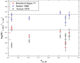
Figure 1: Ratio of theoretical-to-experimental quadratic Stark width versus the effective quantum number of the upper level at $T_{\rm e}=28\,000\;$K. The theoretical widths were calculated using three different approximations with the sources noted in the legend. The dotted lines indicate a factor of two uncertainty.

Table 3: Average ratios of calculated to experimental Stark widths. S88 refers to Seaton (1988), K79 refers to Kurucz (1979), and SB71 refers to Sahal-Bréchot & Segre (1971).

Temperature	Average $\left(\gamma_{\rm calc}/\gamma_{\rm exp}\right)$
(K)	S88	K79	SB71
8000	2.12	0.23	0.71
15000	1.92	0.22	0.61
28000	1.55	0.21	0.40

3.2 N iii & N iv Atomic Data

N iii and N iv energy levels were taken from Moore (1993). In total, the twelve lowest LS levels of N iii and the ground state of N iv were included in the calculation. The oscillator strengths of radiative bound-bound transitions of N iii were obtained from Bell et al. (1995) and Fernley et al. (1999), available from the NIST database. The photoionization cross-sections were also taken from Fernley et al. (1999). Similarly, the collision strengths of excitation and ionization were calculated using impact parameter approximation of Seaton (1962).

4 Calculations

The N ii non-LTE line formation calculation was carried out for all combinations of nine $T_{\rm eff}$, between 15,000 and 31,000 K in steps of 2000 K, three surface gravities, $\log g$ (3.5, 4 and 4.5), four microturbulent velocities, $\xi_{t}$ (0, 2, 5 and $10\;\rm km\,s^{-1}$), and 7 nitrogen abundances, between 6.83 and 8.13 dex. The MULTI code, v2 (Carlsson, 1992), was used. MULTI solves the statistical equilibrium and radiative transfer equations simultaneously in an iterative method using the approximate lambda-operator technique of Scharmer (1981). The option of using a local approximate lambda-operator was used in the current calculations. A solar nitrogen abundance $\epsilon_{N}$= 7.83 was adopted from Grevesse et al. (2010).

The fixed, background model photospheres providing $T(\tau)$ and $P(\tau)$ for the non-LTE calculation were taken from the LTE, line blanketed, atmospheres of ATLAS9 (Kurucz, 1993). ATLAS9 was also used to provide the mean intensity within the stellar atmosphere as a function of optical depth, $J_{\nu}(\tau)$, used to compute all of the photoionization and recombination rates which were kept fixed during the calculations. Using LTE model atmospheres can be a source of error, particularly for hotter stars; however, previous studies have shown that a comprehensive inclusion of line-blanketing is more important than non-LTE effects up to stellar effective temperatures of $\approx\,$30,000 K (Przybilla & Butler, 2001).

As MULTI was originally developed for the atmospheres of cool stars, modification to the background opacities are required in order to be suitable for early-type stars; its default opacity package was replaced with the extensive package that is available through ATLAS9 (Sigut & Lester, 1996).

4.1 Ionization Balance and Departure Coefficients

(a)

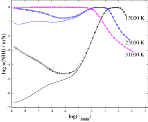
(b)

Figure 2: Panel (a) shows the fraction of N ii as a function of $\log\tau_{5000}$ for several stellar $T_{\rm eff}$ in atmospheres with $\log g$= 4.0, $\xi_{t}=5\;\rm km\,s^{-1}$, and $\epsilon_{N}$= 7.83. The circles represent the non-LTE fraction and solid lines, the LTE fractions. Panel (b) is the same, but for N iii. In both panels, the line colour indicates $T_{\rm eff}$ as 15000 K (black), 23,000 K (blue), and 31,000 K (purple).

Figure 2 shows the predicted LTE and non-LTE ionization fractions of N ii (top panel) and N iii (bottom panel) as a function of the continuum optical depth at $5000\,$Å, $\log\tau_{5000}$, for the range of the $T_{\rm eff}$ considered. These illustrated models assume $\log\,g=4.0$, $\xi_{t}=5\;\rm km\,s^{-1}$, and the solar nitrogen abundance.

At $T_{\rm eff}$ less than $\sim 21,000\,$K, N ii is the dominant ionization stage throughout the formation region of the optical N ii lines, $-2\leq\,\log\tau_{5000}\leq 0$, and there is little deviation from the LTE ionization fraction. Table 1 shows that the six lowest energy levels of N ii have photoionization thresholds shortward of the Lyman limit at 912 Å, which remains optically thick throughout most of the atmosphere. This leads to a strongly local photoionizing radiation field, i.e. $J_{\nu}\,\approx\,B_{\nu}(T_{e})$. It is only by level 7, $2p\,3p\,^{1}D$, that the photoionization threshold begin to lie in the short-wavelength region of the Balmer continuum where the photoionizing radiation field can be both hot and non-local. This high radiation temperature in the Balmer continuum can drive overionization; however, even at the highest $T_{\rm eff}$ considered here, the predicted non-LTE over-ionization of N ii is quite small in the line formation region (Figure 2).

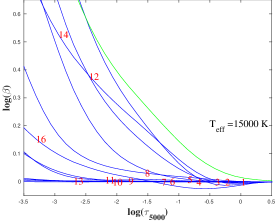
(a)

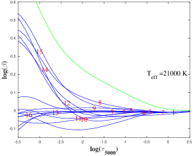
(b)

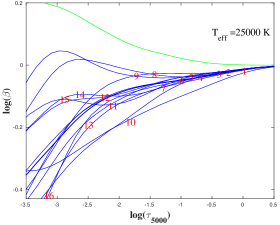
(c)

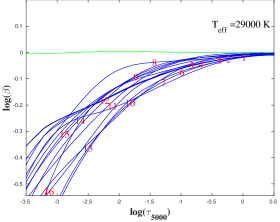
(d)

Figure 3: Non-LTE departures coefficients, $\log\beta_{i}$, for the lowest 16 energy levels of N ii of Table 1 (blue lines identified by level number) and the ground level of N iii (green line) as a function of $\tau_{5000}$. The stellar $T_{\rm eff}$ shown are 15,000 K (panel a), 21,000 K (panel b), 25000 K (panel c), and 29,000 K (panel d). The surface gravity and microturbulent velocity were fixed at $\log\,g=4.0$ and $\xi_{t}=5\;\rm km\,s^{-1}$, and the solar nitrogen abundance was assumed.

The predicted departure coefficients for the 16 lowest LS states of N ii (Table 1) and the ground state of N iii, for four values of $T_{\rm eff}$ in models with $\log g=$ 4.0, $\xi_{t}=5.0\;\rm km\,s^{-1}$, and the solar nitrogen abundance, are shown in Figure 3. The departure coefficient of the $i^{th}$ energy level, $\beta_{i}$, is defined as the ratio of the non-LTE number density to the corresponding LTE value computed by the Saha/Boltzmann equations for the local values of $T_{e}$ and $N_{e}$,

$$\beta_{i}\equiv\frac{n_{i}}{n_{i}^{*}(T_{e},N_{e})}\;,$$ (1)

where $n_{i}^{*}$ and $n_{i}$ are the predicted LTE and non-LTE number densities of the $i^{th}$ level, respectively. Among the levels of particular interest are 9 and 16, the upper and lower levels of $\lambda\,3995$, and 9 and 11, the upper and lower levels of $\lambda\,6482$ (see Table 2). These transitions will be explicitly discussed in the remainder of the text.

At $T_{\rm eff}=15,000\,$K, Figure 3a, all of the low-lying levels ($\leq 10$) are in LTE throughout the atmosphere. As $T_{\rm eff}$ increases, there is a systematic trend for overionization of all of the low-lying levels to set in. This is clear by $T_{\rm eff}=25,000\,$K, Figure 3c, where near $\log\tau_{5000}\approx-0.5$, all of the low-lying levels share the same departure coefficient, $\beta$, due to strong collisional coupling, with $\beta<1$ due to photoionization in the short wavelength portion of the Balmer continuum. By $T_{\rm eff}=25,000\,$K, the upper levels with threshold in this region have sufficient population and N ii is no longer the dominant ionization stage, allowing the overionization to occur. This trend continues for $T_{\rm eff}=29,000\,$K. For $T_{\rm eff}<21,000\,$K, the overpopulation of the N iii ground state leads to general over population of the higher N ii excited states, although this effect diminishes by $T_{\rm eff}=25,000\,$K.

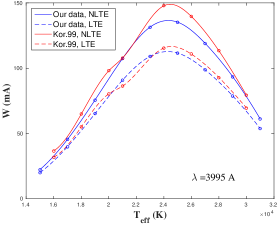
(a)

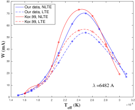
(b)

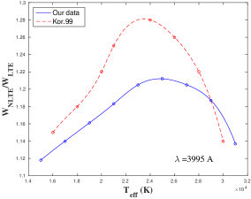
(c)

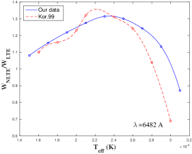
(d)

Figure 4: The LTE and non-LTE equivalent widths of N ii $\lambda\,3995$; (panel a) and $\lambda\,6482$, (panel b) respectively, as a function of $T_{\rm eff}$ for $\log g=$ 4.0, $\xi_{t}=5\;\rm km\,s^{-1}$ and $\epsilon_{N}=$ 7.95. The blue symbols are the current results and the red symbols, Korotin et al. (1999). The two bottom panels, (c) and (d), give the ratio of the non-LTE and LTE equivalent widths.

4.2 N ii Equivalent Widths

Figure 4 shows the predicted LTE and non-LTE equivalent widths (in milli-Å) for N ii $\lambda\,3995$ and $\lambda\,6482$ representing transitions from levels 9 to 16 $(3s\,^{1}P^{o}\rightarrow 3p\,^{3}D)$ and levels 9 to 11 ($3s\,^{1}P^{o}\rightarrow 3p\,^{1}P$), respectively. For comparison, the predictions of Korotin et al. (1999) are also shown. In general, there is reasonable agreement between the two calculations. For $\lambda\,3995$, we find smaller deviations from LTE near the line’s maximum strength at $T_{\rm eff}\approx 25,000\,$K (Figure 4c). For $\lambda\,6482$, agreement is good for $T_{\rm eff}<24,000\,$K; however, for hotter $T_{\rm eff}$, we again predict smaller departures from the LTE equivalent width than Korotin et al. (1999) (Figure 4d).

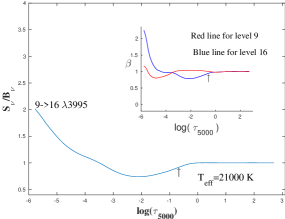
(a)

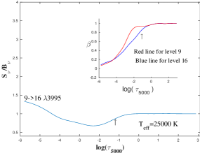
(b)

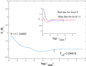
(c)

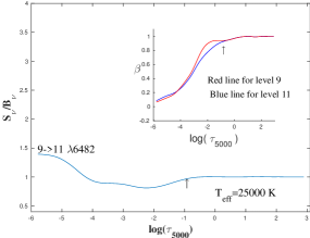
(d)

Figure 5: The line source functions as a function of $\log\tau_{5000}$ for N ii $\lambda\,3995$ and $\lambda\,6482$ at two $T_{\rm eff}$, 21000 and 25000 K. Both models assumed $\log g=4.0$, $\xi_{t}=5\;\rm km\,s^{-1}$ and the solar nitrogen abundance. The departure coefficients of the upper and lower energy levels are shown in the panel inserts. The arrows point to the depth of formation of the line centre flux as defined by the contribution function of X.

In general, the non-LTE equivalent widths are predicted to be larger than the corresponding LTE values. These differences result from deviations of the line source function from the local Planck function and the non-LTE correction to the line optical depth scale. In terms of the departure coefficients of the upper and lower levels, $\beta_{u}$ and $\beta_{l}$, the line source function is

$$S_{l}=\frac{2h\nu^{3}}{c^{2}}\left(\frac{\beta_{l}}{\beta_{u}}e^{\frac{h\nu}{kT}}-1\right)^{-1}\,,$$ (2)

and the line optical depth scale is,

$$d\tau^{l}_{\nu}=-\frac{h\nu}{4\pi}\left(\beta_{l}\,n^{*}_{l}-\beta_{u}\,n^{*}_{u}\right)\,\phi_{\nu}\,dz\,.$$ (3)

Here $\phi_{\nu}$ is the line absorption profile, $n^{*}$ are the LTE level populations, and $dz$ is the physical step (in cm) along the ray. Complete redistribution, the equality of the line emission and absorption profiles, has been assumed (Mihalas, 1978). Note that if $h\nu\gg kT$ (i.e. the photon energy exceeds the local kinetic energy), we have the scalings $S_{l}\propto\beta_{u}/\beta_{l}$ and $d\tau^{l}_{\nu}\propto\beta_{l}$. As the Eddington-Barbier relation states that the emergent intensity is characteristic of the source function at an optical depth of $\approx 2/3$, we see that $\beta_{l}$ affects how deeply we see into the atmosphere, whereas $\beta_{u}/\beta_{l}$ controls the value of the source function at this point. This emphasizes that even in cases where $S_{l}=B_{\nu}(T_{\rm e})$, i.e. $\beta_{u}/\beta_{l}=1$, there can still be large non-LTE effects, for example, if $\beta_{l}=\beta_{u}\ll 1$.

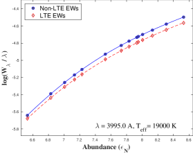
(a)

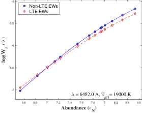
(b)

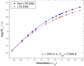
(c)

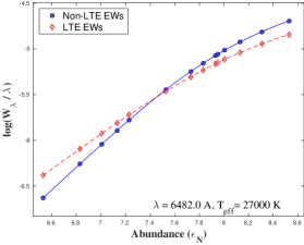
(d)

Figure 6: LTE and non-LTE curves of growth for N ii $\lambda\,6482$ and $\lambda\,3995$ as a function of nitrogen abundance, $\rm\epsilon_{N}$, at the indicated $T_{\rm eff}$ with $\log g$= 4.0, and $\xi_{t}=5\;\rm km\,s^{-1}$. The blue, solid lines represent the predicted non-LTE equivalent widths and the dashed, red, dashed lines represent the corresponding LTE values.

Panels LABEL:sub@Snu_3995_T21000 and LABEL:sub@Snu_3995_T25000 of Figure 5 show the ratio of the line source function to Planck function for N ii $\lambda\,3995$ as a function of $\tau_{5000}$ at two $T_{\rm eff}$, 21,000 and 25,000 K. The departure coefficients of the upper and lower levels are shown as inserts in each figure.

Consider first $\lambda\,3995$, transition $9\rightarrow 16$. The depth of formation of the line centre flux is marked with an arrow, following the flux contribution function proposed by Achmad et al. (1991). At $T_{\rm eff}$ of 21,000 K there is a small overpopulation of the the ninth energy level and a small under-population of the sixteenth level, while at $T_{\rm eff}$ of 25,000 K, there is under-population of both levels. In both cases, the main effect is the larger under-population of the upper energy level which acts to reduce the line source function in the line-forming region leading to non-LTE strengthening of the line. The behaviour of $\lambda\,6482\,$Å, transition $9\rightarrow 11$, is qualitatively similar. However, for $T_{\rm eff}$ greater than 28,000 K, there is a non-LTE weakening of the line driven by the overionization of N ii in such models.

For both $\lambda\,3995$ and $\lambda\,6482$, non-LTE strengthening of the lines reaches a maximum near $T_{\rm eff}\approx 25,000\;$K where the lines are about 20% and 30% stronger than the LTE predictions, respectively (Figures 4a and 4b). This overall behaviour is in agreement with the calculation of Korotin et al. (1999), although our overall non-LTE strengthening of $\lambda\,3995$ is less and our non-LTE weakening of $\lambda\,6482\,$Å for high $T_{\rm eff}$ is also less. The stronger non-LTE effects seen by Korotin et al. (1999) may reflect their lower number of bound-bound radiative transitions included, 266 transitions in total, with 92 included in the linearization procedure and the rest kept at fixed rates. In the current work, a total of 580 radiative transitions were included, none with fixed rates, representing all LS transitions with oscillator strengths greater than or equal to $10^{-3}$. We confirm that it is the larger number of radiative transitions included in the present work that explains most of the differences with K99 by constructing a 43 LS level N ii atom that includes the same set of allowed rbb transitions as K99. Using this atom, their non-LTE equivalent widths could be reproduced with a good agreement as a function of $T_{\rm eff}$ for the model $\log g$= 4.0, $\xi_{t}=5\,\rm km\,s^{-1}$ and $\epsilon_{N}=7.95$, Table (5) in K99.

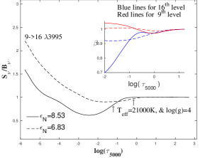
(a)

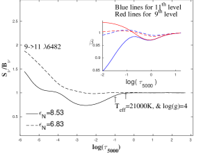
(b)

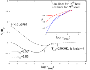
(c)

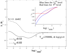
(d)

Figure 7: The source functions of the N ii $\lambda\,3995$ for two different nitrogen abundances, $\epsilon_{N}=6.83$ (solid lines) and $8.53$ (dashed lines). The $T_{\rm eff}$ and $\log\,g$ of the models are as indicated. The microturbulent velocity was $\xi_{t}=5\;\rm km\,s^{-1}$.

There is also a dependence of the size of the predicted non-LTE effects on the nitrogen abundance. This is illustrated in Figure 6 which show curves of growth, $\log(W_{\lambda}/\lambda)$ versus $\epsilon_{N}$, for both $\lambda\,3995$ and $\lambda\,6482$ at two $T_{\rm eff}$, 19,000 K and 27,000 K. A gravity of $\log\,g=4.0$ and a microturbulent velocity of $\xi_{t}=5\;\rm km\,s^{-1}$ were assumed for all examples. For $\lambda\,3995$, there is non-LTE strengthening at all nitrogen abundances, with the largest effect at the highest abundance considered. For $\lambda\,6482$, there is a reversing trend with non-LTE weakening predicted for small abundances and a non-LTE strengthening at larger abundances. The transition occurs at abundances somewhat less than the solar value.

This abundance effect is further explored in Figure 7 which shows the line source functions and departure coefficients of both $\lambda\,3995$ and $\lambda\,6482$ at the two extreme values of the nitrogen abundance considered, $\epsilon_{N}=6.83$ ($-1.0\;$dex relative to solar) and $\epsilon_{N}=8.53$ ($+0.7\;$dex relative to solar). The figure shows that the increase of the nitrogen abundance reduces the line source function value and shifts the line formation regions to smaller optical depths ($\log\tau_{5000}$).

Grids of non-LTE equivalent widths for $\lambda\,3995$ and $\lambda\,6482$ over all $T_{\rm eff}$, $\log\,g$ and $\epsilon_{N}$ considered are given in Tables 9 and 10. The microturbulent velocity was set to $5\;\rm km\,s^{-1}$. Full grids of equivalent widths for all transitions of Table 2 over all models and microturbulences considered are available on-line.

Finally we note that the equivalent width of $\lambda\,6482$ at the highest temperature considered in Table 10, 31,000 K, becomes weakly negative, indicating line emission. This is a well-known non-LTE effect that can occur when $h\nu/kT\ll 1$: the source function becomes very sensitive to small departures from LTE and can rise in the outer layers, even though the photospheric temperature falls with height. This effect is extensively discussed in Carlsson et al. (1992) and Sigut & Lester (1996).

4.3 A Multi-MULTI Analysis

In order to investigate which of the radiative and collisional transitions included in the atom have the most significant effects on the predicted equivalent widths of the N ii lines of interest, a series of multi-MULTI analysis were carried out (Carlsson et al., 1992). In a multi-MULTI analysis, a single radiative or collisional transition is perturbed by doubling its rate, and a new converged solution is obtained for the perturbed atom. The predicted equivalent widths from this new converged solution are compared with the reference solution of the unperturbed atom. Table 4 shows the top ten radiative/collisional transitions affecting the predicted equivalent widths of $\lambda\,6482$ and $\lambda\,3995$ for $\rm T_{eff}\,$= 23,000 K, $\log g$= 4.0, $\xi_{t}\,=$5 $\rm km\,s^{-1}$, and a solar nitrogen abundance. Corresponding to Table 4, Figure 8a shows the effect on the line source function and upper and lower level departure coefficients of the top four rates for $\lambda\,3995$.

Table 4: multi-MULTI Analysis at $\rm T_{eff}$= 23000 K, $\log g$=4.0, and $\xi_{t}=5.0\;\rm km\,s^{-1}$

Transition	Perturbed transition					Type	$\%$
3995.0 Å	9	$\rightarrow$	16	($2p\;3s\;^{1}P^{o}$	-$2p\;3p\;^{1}D$)	rbb	35.22
	16	$\rightarrow$	94	($2p\;3p\;^{1}D$	-$2s^{2}\;2p\;^{2}P^{o}$ N iii)	rbf	1.67
	9	$\rightarrow$	16	($2p\;3s\;^{1}P^{o}$	-$2p\;3p\;^{1}D$)	cbb	-1.43
	16	$\rightarrow$	87	($2p\;3p\;^{1}D$	-$\rm high\;l,n=6$)	rbb	-1.29
	16	$\rightarrow$	22	($2p\;3p\;^{1}D$	-$2p\;3d\;^{1}F^{o}$)	rbb	-1.21
	22	$\rightarrow$	87	($2p\;3d\;^{1}F^{o}$	-$\rm high\;l,n=6$)	rbb	-0.94
	8	$\rightarrow$	94	($2p\;3s\;^{3}P^{o}$	-$2s^{2}\;2p\;^{2}P^{o}$ N iii)	rbf	-0.79
	16	$\rightarrow$	25	($2p\;3p\;^{1}D$	-$2p\;4s\;^{1}P^{o}$)	rbb	-0.75
	1	$\rightarrow$	94	($2p^{2}\;{}^{3}P$	-$2s^{2}\;2p\;^{2}P^{o}$ N iii)	rbf	0.71
	12	$\rightarrow$	16	($2p\;3p\;^{3}D$	-$2p\;3p\;^{1}D$)	cbb	-0.68
6482.0 Å	9	$\rightarrow$	11	($2p\;3s\;^{1}P^{o}$	-$2p\;3p\;^{1}P$)	rbb	71.67
	11	$\rightarrow$	19	($2p\;3p\;^{1}P$	-$2p\;3d\;^{1}D^{o}$)	rbb	-6.45
	11	$\rightarrow$	94	($2p\;3p\;^{1}P$	-$2s^{2}\;2p\;^{2}P^{o}$ N iii)	rbf	3.95
	9	$\rightarrow$	16	($2p\;3s\;^{1}P^{o}$	-$2p\;3p\;^{1}D$)	rbb	3.41
	9	$\rightarrow$	11	($2p\;3s\;^{1}P^{o}$	-$2p\;3p\;^{1}P$)	cbb	-3.12
	11	$\rightarrow$	23	($2p\;3p\;^{1}P$	-$2p\;3d\;^{1}P^{o}$)	rbb	-2.95
	19	$\rightarrow$	87	($2p\;3d\;^{1}D^{o}$	-$\rm high\;l,n=6$)	rbb	-2.91
	7	$\rightarrow$	11	($2p^{3}\;{}^{1}D^{o}$	-$2p\;3p\;^{1}P$)	rbb	2.92
	1	$\rightarrow$	6	($2p^{2}\;{}^{3}P$	-$2p^{3}\;{}^{3}P^{o}$)	rbb	-2.03
	1	$\rightarrow$	6	($2p^{2}\;{}^{3}P$	-$2p^{3}\;{}^{3}P^{o}$)	cbb	2.00

Note: rbb and rbf refer to bound-bound and bound-free radiative transitions, respectively, and cbb and cbf refer to bound-bound and bound-free collisional transitions, respectively.

For $\lambda\,3995$, the equivalent width is most sensitive to its own radiative transition rate controlled by the oscillator strength; e.g. doubling the oscillator strength of the $\lambda\,3995$ line leads to $\approx$ 40% increase in the predicted equivalent width. The increased oscillator strengths shifts the depth of formation of the line to smaller optical depths ($\log\tau_{5000}$) where the line source function is lower, leading to an increase in the line strength. Next in importance was the photoionization rate from the upper level of $\lambda\,3995$ (level 16). An increase in this rate by a factor of two leads to an increase in the predicted non-LTE equivalent width of $\approx\,2$%. Increased photoionization from the upper level again acts to reduce the line source function in the line-forming regions. The collisional bound-bound transition between the lower and upper energy levels of the $\lambda\,3995$ (the ninth energy level, and the sixteenth energy level) is next in importance. Doubling the strength of this collisional bound-bound transition increases the collisional coupling between these two levels, and increased collisional coupling tends to force LTE, i.e. $S_{\nu}$ comes closer to $B_{\nu}$ in Figure 8c; this raises the source function in the line forming region and therefore the line is weaker.

Table 5: multi-MULTI Analysis at $\rm T_{eff}$= 15000 K, $\log g$=4.0, and $\xi_{t}=5.0\;\rm km\,s^{-1}$

Transition	Perturbed transition					Type	$\%$
3995.0 Å	9	$\rightarrow$	16	($2p\;3s\;^{1}P^{o}$	-$2p\;3p\;^{1}D$)	rbb	59.47
	9	$\rightarrow$	16	($2p\;3s\;^{1}P^{o}$	-$2p\;3p\;^{1}D$)	cbb	-1.35
	12	$\rightarrow$	16	($2p\;3p\;^{3}D$	-$2p\;3p\;^{1}D$)	cbb	-0.75
	8	$\rightarrow$	16	($2p\;3s\;^{3}P^{o}$	-$2p\;3p\;^{1}D$)	rbb	0.52
	11	$\rightarrow$	16	($2p\;3p\;^{1}P$	-$2p\;3p\;^{1}D$)	cbb	-0.50
	8	$\rightarrow$	16	($2p\;3s\;^{3}P^{o}$	-$2p\;3p\;^{1}D$)	cbb	-0.43
	16	$\rightarrow$	22	($2p\;3p\;^{1}D$	-$2p\;3d\;^{1}F^{o}$)	rbb	-0.35
	16	$\rightarrow$	25	($2p\;3p\;^{1}D$	-$2p\;4s\;^{1}P^{o}$)	rbb	-0.33
	16	$\rightarrow$	22	($2p\;3p\;^{1}D$	-$2p\;3d\;^{1}F^{o}$)	cbb	-0.33
	15	$\rightarrow$	16	($2p\;3p\;^{3}P$	-$2p\;3p\;^{1}D$)	cbb	-0.25
6482.0 Å	9	$\rightarrow$	11	($2p\;3s\;^{1}P^{o}$	-$2p\;3p\;^{1}P$)	rbb	105.76
	11	$\rightarrow$	14	($2p\;3p\;^{1}P$	-$2p\;3p\;^{3}S$)	cbb	-4.30
	11	$\rightarrow$	19	($2p\;3p\;^{1}P$	-$2p\;3d\;^{1}D^{o}$)	rbb	-3.87
	8	$\rightarrow$	14	($2p\;3s\;^{3}P^{o}$	-$2p\;3p\;^{3}S$)	rbb	3.61
	9	$\rightarrow$	16	($2p\;3s\;^{1}P^{o}$	-$2p\;3p\;^{1}D$)	rbb	3.27
	1	$\rightarrow$	6	($2p^{2}\;{}^{3}P$	-$2p^{3}\;{}^{3}P^{o}$)	rbb	-2.15
	1	$\rightarrow$	6	($2p^{2}\;{}^{3}P$	-$2p^{3}\;{}^{3}P^{o}$)	cbb	2.15
	11	$\rightarrow$	16	($2p\;3p\;^{1}P$	-$2p\;3p\;^{1}D$)	cbb	2.06
	8	$\rightarrow$	12	($2p\;3s\;^{3}P^{o}$	-$2p\;3p\;^{3}D$)	rbb	1.89
	7	$\rightarrow$	11	($2p^{3}\;{}^{1}D^{o}$	-$2p\;3p\;^{1}P$)	rbb	1.72

Similar results were obtained for the multi-MULTI analysis of the $\lambda\,6482$. Doubling the oscillator strength of the radiative transition itself causes an increase in the equivalent width by $\approx$ 60%, while doubling the collision strength of this transition reduces the predicted non-LTE line strengthening and the non-LTE equivalent width by $\approx$ 2%.

Tables 5 and 6 show the results of a multi-MULTI analysis for the same two N ii transitions but at $T_{\rm eff}=15,000$ and $29,000\;$K. At $\rm T_{eff}=15,000\;$K, the radiative bound-free transitions play little important role as N ii is the dominant ionization stage in the line forming region and changes in the radiative bound-free (rbf) rates have only have only a minor effects on the N ii populations. At $\rm T_{eff}=29,000\;$K, the rbf transitions play a much more important role as N iii is the dominant ionization stage of the nitrogen atom.

Table 6: multi-MULTI Analysis at $\rm T_{eff}$= 29000 K, $\log g$=4.0, and $\xi_{t}=5.0\;\rm km\,s^{-1}$

Transition	Perturbed transition					Type	$\%$
3995.0 Å	9	$\rightarrow$	16	($2p\;3s\;^{1}P^{o}$	-$2p\;3p\;^{1}D$)	rbb	57.66
	16	$\rightarrow$	94	($2p\;3p\;^{1}D$	-$2s^{2}\;2p\;^{2}P^{o}$ N iii)	rbf	7.95
	1	$\rightarrow$	94	($2p^{2}\;{}^{3}P$	-$2s^{2}\;2p\;^{2}P^{o}$ N iii)	rbf	6.83
	2	$\rightarrow$	94	($2p2\;0p\;^{1}D$	-$2s^{2}\;2p\;^{2}P^{o}$ N iii)	rbf	5.62
	9	$\rightarrow$	11	($2p\;3s\;^{1}P^{o}$	-$2p\;3p\;^{1}P$)	rbb	5.34
	9	$\rightarrow$	12	($2p\;3s\;^{1}P^{o}$	-$2p\;3p\;^{3}D$)	rbb	4.97
	11	$\rightarrow$	19	($2p\;3p\;^{1}P$	-$2p\;3d\;^{1}D^{o}$)	rbb	4.97
	4	$\rightarrow$	94	($2p^{3}\;{}^{5}S^{o}$	-$2s^{2}\;2p\;^{2}P^{o}$ N iii)	rbf	4.96
	8	$\rightarrow$	16	($2p\;3s\;^{3}P^{o}$	-$2p\;3p\;^{1}D$)	rbb	4.96
	9	$\rightarrow$	15	($2p\;3s\;^{1}P^{o}$	-$2p\;3p\;^{3}P$)	rbb	4.80
6482.0 Å	9	$\rightarrow$	11	($2p\;3s\;^{1}P^{o}$	-$2p\;3p\;^{1}P$)	rbb	125.08
	11	$\rightarrow$	94	($2p\;3p\;^{1}P$	-$2s^{2}\;2p\;^{2}P^{o}$ N iii)	rbf	24.15
	9	$\rightarrow$	16	($2p\;3s\;^{1}P^{o}$	-$2p\;3p\;^{1}D$)	rbb	18.65
	1	$\rightarrow$	94	($2p^{2}\;{}^{3}P$	-$2s^{2}\;2p\;^{2}P^{o}$ N iii)	rbf	16.16
	19	$\rightarrow$	94	($2p\;3d\;^{1}D^{o}$	-$2s^{2}\;2p\;^{2}P^{o}$ N iii)	rbf	14.79
	7	$\rightarrow$	11	($2p^{3}\;{}^{1}D^{o}$	-$2p\;3p\;^{1}P$)	rbb	14.41
	2	$\rightarrow$	94	($2p^{2}\;{}^{1}D$	-$2s^{2}\;2p\;^{2}P^{o}$ N iii)	rbf	12.94
	9	$\rightarrow$	12	($2p\;3s\;^{1}P^{o}$	-$2p\;3p\;^{3}D$)	rbb	12.15
	8	$\rightarrow$	11	($2p\;3s\;^{3}P^{o}$	-$2p\;3p\;^{1}P$)	rbb	11.44
	9	$\rightarrow$	15	($2p\;3s\;^{1}P^{o}$	-$2p\;3p\;^{3}P$)	rbb	11.37

(a)

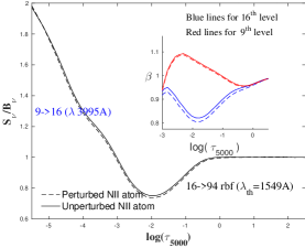
(b)

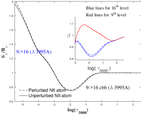
(c)

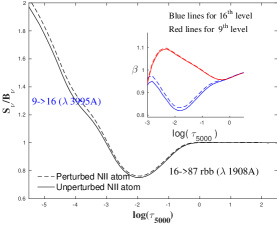
(d)

Figure 8: The line source function of N ii $\lambda\,3995$ line for the perturbed nitrogen atom and the departure coefficients of the upper and lower energy levels of this transition (dashed lines) for $\rm T_{eff}=$ 23000 K, $\log g=$ 4.0, $\xi_{t}=5\;\rm km\,s^{-1}$, and $\rm\epsilon_{N,solar}$= 7.83. For comparison the results of the unperturbed atom were added (solid lines), where the perturbed transition is displayed in the lower right corner of each panel.

4.4 A Monte-MULTI Analysis

The accuracy of a non-LTE line formation calculation depends on many factors, and an important one is the accuracy and completeness of the basic atomic data used. The inclusion of atomic data from many different sources, all with different accuracies, represents a source of random errors in the estimated equivalent widths. In order to quantify these errors, a series of Monte Carlo simulations were carried out following the procedure developed by Sigut (1996). Two hundred random realizations of the nitrogen atom were generated with the atomic data varied within the bounds given in Table 7. The choices for the adopted uncertainties in the atomic data are justified as follows:

• The oscillator strengths ($\it f$-values) of the bound-bound radiative transitions were varied within $\pm$10 % for ${\it f}\geq 0.1$ and $\pm$50 % for weaker transitions. These values were chosen because the Opacity Project length and velocity $\it f$-values differ by approximately these ranges. The difference between these two equivalent formalisms, length and velocity, is a measure of the accuracy of the calculation (Froese Fischer et al., 2000).

• Stark damping widths were allowed to vary within $\pm$40 %, which is on the order of the difference between our calculated Stark widths using the OP formalism of Seaton (1988) and the available experimental values– see Table 3.

• The photoionization cross sections were allowed to vary within $\pm$20$\%$. OP photoionization cross sections have uncertainties of $\approx\,$10 % (Yan & Seaton, 1987) but this range was doubled to account for possible errors in the photoionizing radiation field predicted by the LTE, line-blanketed model atmospheres and used in the calculation of the (fixed) photoionization rates.

• Thermally-averaged collision strengths were allowed to vary over a range determined by their source. The $\cal R$-matrix method represents an accurate way to compute thermally-averaged collisional strengths at low temperatures for low-lying levels in an ion. Hudson & Bell (2004) show that their results agree with the the results of previous R-matrix calculations within $\rm\approx\,10\,\%$, which we adopt as the uncertainty in such collision strengths. For majority of radiatively-allowed transitions without ${\cal R}$-matrix collision strengths, the impact parameter method Seaton (1962) was used, and a factor of two uncertainly was employed. Note that Sigut & Lester (1996) compared ${\cal R}$-matrix collision strengths to impact parameter predictions in the case of Mg ii and found about a factor of 2 in accuracy.

• Collisional ionization rates are highly uncertain and the very crude approximation of Seaton (1962) was used for all rates. An uncertainty of a factor of 5 was assigned to all such values.

Table 7: Rates of variation of the atomic data

Atomic parameter	Uncertainty
$\it f$-value	$\pm$ 10% $\it f$-value $\geq$ 0.1
	$\pm$ 50% $\it f$-value $<$0.1
Stark widths	$\pm$ 40%
Photoionization cross section	$\pm$ 20%
Collision strength (Excitation)
R-Matrix	$\pm$ 10%
Impact parameter	Factor of 2
Collisional strength (Ionization)	Factor of 5

A converged non-LTE solution was found for each of the 200 randomly-realized atoms, and the distribution of the predicted equivalent widths was taken to estimate the uncertainty. Example distributions for $\lambda\,3995$ and $\lambda\,6482$ are shown in Figure 9 for the models with $T_{\rm eff}=19,000$ and 23,000 K, with $\log g=4.0$, $\xi_{t}=5\;\rm km\,s^{-1}$ and the solar nitrogen abundance. A Gaussian fit to each distribution gives the standard deviation and hence the associated uncertainty due to inaccuracies in the atomic data (taken to be $2\,\sigma$). Tabular results are given in Table 12 for both transitions with $T_{\rm eff}$’s between 15000 and 31000, and nitrogen abundances between 6.83 and 8.13. Tables 11 and 13 in appendix B show the results of Monte Carlo simulations for $\log g=\,$3.5 and 4.5, and $\xi=\,5.0\;\rm km\,s^{-1}$, over the range of $T_{\rm eff}$ considered; given in each of these tables is the average equivalent width of each transition and its $2\sigma$ variation.

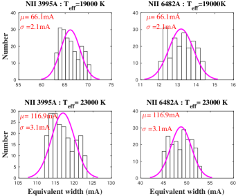
Figure 9: The equivalent width distribution for the 200 N ii model atoms for $\lambda\,6482$ and $\lambda\,3995$ at $\rm T_{eff}$= 19000 and 23000 K, $\log g$, equal to 4.0, $\xi_{t}=5\;\rm km\,s^{-1}$, and solar nitrogen abundance were assumed.

In addition to the uncertainty itself, these random realizations allow one to determine which individual rates most affect the uncertainty in each transition’s equivalent width. This is different from the previous multi-MULTI calculation as a realistic uncertainty for each rate is used, as opposed to an arbitrary doubling. However, as the individual rates are not varied one at a time, it is necessary to look at the correlations between the equivalent width of the transition of interest and the 200 scalings of each rate. The largest correlation coefficients of the N ii $\lambda\,3995$ and $\lambda\,6482$ equivalent widths at $T_{\rm eff}$ of 19,000, 23,000 and 27,000 K, $\log\,g=4.0$, $\xi_{t}=5\;\rm km\,s^{-1}$, and the solar nitrogen abundance are shown in Table (8). For 200 random realizations, a correlation coefficient of 0.18 is a statistical significant at 1% level (Bevington, 1969). The variation in the predicted equivalent widths of both transitions is most strongly correlated with the variations in that transition’s oscillator strength, as expected. The remainder of the strongest correlations, at the level of $|r|\sim 0.22$, are with collisional bound-bound rates between higher excitation levels. This reflects the large uncertainties assigned to these rates as compared to the oscillator strengths and $\cal R$-matrix collision strengths (see Table 7).

4.5 Limiting Accuracy of Nitrogen Abundances

Finally, in order to quantify the ultimate accuracy of determined nitrogen abundances due to uncertainties in the atomic data, the equivalent widths predicted by the unperturbed atom for three singlet lines, $\lambda\,3995$, $\lambda\,4447$ and $\lambda\,6482$, were used as reference “observed" equivalent widths for each $T_{\rm eff}$ assuming $\log\,g=4.0$ and $\xi_{t}=5\;\rm km\,s^{-1}$. Then the curves of growth for each of the 200 randomly-realized atoms were used to derive a nitrogen abundance based on exactly the same stellar parameters and microturbulent value, i.e. the ideal case. The dispersion in the abundances obtained from the 200 curves-of-growth can then be taken as the limiting uncertainty in the derived nitrogen abundance due to atomic data limitations. This process was then repeated for all nitrogen abundances in the range considered, $\epsilon_{\rm N}=6.58$ to 8.53. The results for four $T_{\rm eff}$ are shown in Figure 10.

The figure shows that abundances obtained using the results of the Monte Carlo simulations match the original abundances, and that the errors in the estimated nitrogen abundances due to uncertain atomic data increase with nitrogen abundance. For example, at $\rm T_{eff}=$ 23,000 K, the uncertainty is $\rm\delta\epsilon=\pm 0.02\,$dex for $\rm\epsilon_{N}=6.83\,$dex which rises to $\rm\delta\epsilon=\pm 0.11\,$dex for $\rm\epsilon_{N}=8.13$ dex.

Figure 10 also shows that the estimated errors also vary with $T_{\rm eff}$. At the same nitrogen abundance, such as $\epsilon_{N}=7.83\,$dex, the abundance uncertainty is $\rm\delta\epsilon=\pm 0.05\,$dex for $\rm T_{eff}=19,000\;$K, $\rm\delta\epsilon=\pm 0.07\,$dex for $\rm T_{eff}=23,000\;$K and $\rm\delta\epsilon=\pm 0.05\,$dex for $\rm T_{eff}=29,000\;$K. The highest error occurs for $\rm T_{eff}$ between 23,000 K and 25,000 K. In addition, including uncertainty in $\rm T_{eff}$ of $\pm 1000.0\,$K causes additional uncertainty in the estimated abundance by a factor of up to $\approx\pm 0.1\,$dex at the lowest temperatures, while uncertainty in $\log g$ by $\pm 0.25\,$dex adds additional uncertainty up to $\pm 0.05\,$dex in the estimated uncertainty of abundance.

Figure 10: Nitrogen abundances determined from the curves-of-growth constructed from the 200 randomly realized atoms using the equivalent widths of $\lambda\,3995$, $\lambda\,4447$ and $\lambda\,6482$ as the input observed values. Four $T_{\rm eff}$ are shown and results were determined for a range of nitrogen abundances. The error bars represent the uncertainties of the estimated abundances due to inaccuracies in the atomic data at $2\,\sigma$. The blue dashed line represents a difference of zero.

Table 8: Results of Monte Carlo Simulations for N ii at $\log g$=4.0, $\xi_{t}=5.0\;\rm km\,s^{-1}$, and solar nitrogen abundance ($\rm\epsilon_{N,solar}=7.83$): Correlation Coefficients

$\lambda$	$\rm T_{eff}$	Perturbed Transition					Type	r
(Å)	(K)
3995	19000	9	$\rightarrow$	16	($2p\;3s\;^{1}P^{o}$	-$2p\;3p\;^{1}D$)	rbb	0.988
		37	$\rightarrow$	55	($2p\;4f\;^{1}F$	-$2p\;5d\;^{1}D^{o}$)	cbb	-0.271
		28	$\rightarrow$	35	($2p\;4p\;^{3}P$	-$2p\;4d\;^{3}D^{o}$)	cbb	0.235
		9	$\rightarrow$	16	($2p\;3s\;^{1}P^{o}$	-$2p\;3p\;^{1}D$)	stk	0.222
		94	$\rightarrow$	104	($2s^{2}\;2p\;^{2}P^{o}$ N iii	-$2s^{2}\;3d\;^{2}D$ N iii)	cbb	0.221
	23000	9	$\rightarrow$	16	($2p\;3s\;^{1}P^{o}$	-$2p\;3p\;^{1}D$)	rbb	0.983
		37	$\rightarrow$	55	($2p\;4f\;^{1}F$	-$2p\;5d\;^{1}D^{o}$)	cbb	-0.270
		28	$\rightarrow$	35	($2p\;4p\;^{3}P$	-$2p\;4d\;^{3}D^{o}$)	cbb	0.234
		94	$\rightarrow$	104	($2s^{2}\;2p\;^{2}P^{o}$ N iii	-$2s^{2}\;3d\;^{2}D$ N iii)	cbb	0.228
		8	$\rightarrow$	49	($2p\;3s\;^{3}P^{o}$	-$2p\;5p\;^{3}D$)	cbb	-0.223
	27000	9	$\rightarrow$	16	($2p\;3s\;^{1}P^{o}$	-$2p\;3p\;^{1}D$)	rbb	0.967
		37	$\rightarrow$	55	($2p\;4f\;^{1}F$	-$2p\;5d\;^{1}D^{o}$)	cbb	-0.265
		94	$\rightarrow$	104	($2s^{2}\;2p\;^{2}P^{o}$ N iii	-$2s^{2}\;3d\;^{2}D$ N iii)	cbb	0.234
		8	$\rightarrow$	49	($2p\;3s\;^{3}P^{o}$	-$2p\;5p\;^{3}D$)	cbb	-0.231
		28	$\rightarrow$	35	($2p\;4p\;^{3}P$	-$2p\;4d\;^{3}D^{o}$)	cbb	0.225
6482	19000	9	$\rightarrow$	11	($2p\;3s\;^{1}P^{o}$	-$2p\;3p\;^{1}P$)	rbb	0.988
		14	$\rightarrow$	73	($2p\;3p\;^{3}S$	-$2p\;6s\;^{3}P^{o}$)	cbb	-0.244
		55	$\rightarrow$	94	($2p\;5d\;^{1}D^{o}$	-$2s^{2}\;2p\;^{2}P^{o}$ N iii)	cbf	0.227
		47	$\rightarrow$	77	($2p\;5s\;^{1}P^{o}$	-$2p\;6p\;^{1}P$)	rbb	-0.219
		56	$\rightarrow$	94	($2p\;5d\;^{3}D^{o}$	-$2s^{2}\;2p\;^{2}P^{o}$ N iii)	cbf	-0.218
	23000	9	$\rightarrow$	11	($2p\;3s\;^{1}P^{o}$	-$2p\;3p\;^{1}P$)	rbb	0.969
		14	$\rightarrow$	73	($2p\;3p\;^{3}S$	-$2p\;6s\;^{3}P^{o}$)	cbb	-0.251
		55	$\rightarrow$	94	($2p\;5d\;^{1}D^{o}$	-$2s^{2}\;2p\;^{2}P^{o}$ N iii)	cbf	0.231
		47	$\rightarrow$	77	($2p\;5s\;^{1}P^{o}$	-$2p\;6p\;^{1}P$)	rbb	-0.210
		56	$\rightarrow$	80	($2p\;5d\;^{3}D^{o}$	-$2p\;6p\;^{3}P$)	stk	-0.210
	27000	9	$\rightarrow$	11	($2p\;3s\;^{1}P^{o}$	-$2p\;3p\;^{1}P$)	rbb	0.910
		14	$\rightarrow$	73	($2p\;3p\;^{3}S$	-$2p\;6s\;^{3}P^{o}$)	cbb	-0.252
		55	$\rightarrow$	94	($2p\;5d\;^{1}D^{o}$	-$2s^{2}\;2p\;^{2}P^{o}$ N iii)	cbf	0.225
		20	$\rightarrow$	43	($2p\;3d\;^{3}D^{o}$	-$2p\;4f\;^{3}D$)	rbb	-0.216
		56	$\rightarrow$	80	($2p\;5d\;^{3}D^{o}$	-$2p\;6p\;^{3}P$)	stk	-0.213

Notes: All correlation coefficients are statistically significant to less than 1% level, and "stk" refers to variation of the Stark width of the radiative transition.

4.6 Possible Systematic Errors

Systematic errors are more difficult to quantify than the random errors in the atomic data. Possible systematic errors can originate from many sources, such the use of LTE stellar atmospheres with fixed elemental abundances, fixed photoionization rates, and a truncated atomic model in terms of included energy levels.

Widely available non-LTE stellar atmosphere models do not readily provide grids of $J_{\nu}$ as a function of optical depth needed for calculating the photoionization rates. On the other side, the opacity distribution function treatment of Kurucz (1979) provides $J_{\nu}$ over manageable grids; this issue is discussed by Przybilla & Butler (2001).

Another source of systematic error is the completeness of the nitrogen atom. Using atomic models with only a few energy levels can result in large non-LTE effects, particularly for trace ions with low-lying levels with photoionization thresholds in the short-wavelength region of the Balmer continuum. Such calculations can predict too much overionization in small atomic models because collisional coupling to the dominant continuum is artificially suppressed (Sigut, 1996). On the other hand, there is a physical limit to how many energy levels can be straightforwardly added to a non-LTE calculation; highly excited levels are only weakly coupled to their parent ion and can be disrupted by the surrounding plasma. This is most naturally described by introducing an occupation probability, between 0 and 1, for each bound level to exist (Hummer & Mihalas, 1988) and reformulating the statistical equilibrium equations to include the occupation probabilities (Hubeny et al., 1994).

In order to test our N ii atom for completeness, we have systematically increased the number of included N ii energy levels from 93 to 150, and for each increase, recomputed the non-LTE solution. Figure 11 shows the effect on the equivalent widths of $\lambda\,3995$ and $\lambda\,6482$. The effect is quite small, a few percent at most, and hence we do not consider the size of the N ii atom used in the present work to be a significant source of uncertainty for the transitions of focus. This lack of strong dependence on the number of non-LTE levels is consistent with the nature of the non-LTE effects in N ii. Because the photoionization thresholds of low-lying N ii levels are in the Lyman continuum, there is little predicted non-LTE overionization in the line forming region and hence collisional coupling to the parent N iii continuum is less important.

Figure 11: The change in the predicted equivalent widths of $\lambda\,3995$ and $\lambda\,6482$ with an increasing number of levels in the nitrogen atom at $\rm T_{eff}=$ 23,000 K, $\log g=$ 4.0, $\xi_{t}=5\;\rm km\,s^{-1}$, and the solar nitrogen abundance.

5 Discussion and Conclusion

We have presented new, non-LTE line calculations for N ii, using the MULTI code of Carlsson (1992), over the range of stellar $T_{\rm eff}$, $\log\,g$, and microturbulent velocities appropriate to the main sequence B stars. Grids of equivalent widths for commonly-used, strong N ii lines in elemental abundance analysis have been provided. A detailed error analysis was performed, and the error bounds on the tabulated equivalent widths due to atomic data uncertainties provided.

We find reasonable agreement with the most recently, tabulated non-LTE equivalents widths, those of Korotin et al. (1999), but, in general, we find weaker non-LTE effects. We attribute this to the much larger number of radiative bound-bound transitions explicitly included in the non-LTE calculation, as opposed to treating many weaker transitions with fixed rates. In addition, our careful treatment of quadratic Stark broadening makes our N ii equivalent widths more reliable at their maximum strengths.

We systematically investigated the completeness of our atomic model in terms of included energy levels. In addition, an extensive Monte-MULTI calculation quantified the effect of atomic data limitations on the N ii equivalent width predictions. In general, near their peak strengths, we find that the limiting accuracy of using non-LTE equivalents widths computed with existing atomic data is $\approx\pm 0.1\;$dex, although this range is somewhat larger for the highest $T_{\rm eff}$ considered.

To be most applicable to main sequence B stars, the effect of gravitational darkening, particularly the latitude-dependent $T_{\rm eff}$, on the optical N ii spectrum should be investigated, and for the Be stars, the potential of disk emission should be quantified. These effects will be investigated in a subsequent work.

This work is supported by the Canadian Natural Sciences and Engineering Research Council (NESRC) through a Discovery Grant to TAAS.

Appendix A Equivalent Widths

This appendix contains the non-LTE equivalent widths (in mÅ) for N ii transitions $\lambda\,3995$ and $\lambda\,6482$ as a function of $T_{\rm eff}$, $\log\,g$, and nitrogen abundance, all for a microturbulence of $\xi_{t}=5\;\rm km\,s^{-1}$. The tabulated widths are those of the unperturbed atom. Equivalent widths for the other transitions in Table 2, and for other $\xi_{t}$ values, are given in the on-line tables.

Table 9: Non-LTE equivalent widths (in mÅ) for N ii $\lambda$ 3995 Å at $\xi_{t}=5\;\rm km\,s^{-1}$. These equivalent widths are for the unperturbed reference atom.

$\rm T_{eff}(\rm K)$, $\log g$	$\rm\Delta\,\epsilon_{N}=\epsilon_{N}-7.83$
	-1.00		-0.70		-0.60		-0.30		0.00		+0.18		+0.30
	$W_{\lambda}$	$W/W_{*}$	$W_{\lambda}$	$W/W_{*}$	$W_{\lambda}$	$W/W_{*}$	$W_{\lambda}$	$W/W_{*}$	$W_{\lambda}$	$W/W_{*}$	$W_{\lambda}$	$W/W_{*}$	$W_{\lambda}$	$W/W_{*}$
15000 , 3.5	6.4	1.11	11.2	1.13	13.2	1.14	21.2	1.16	32.1	1.17	40.1	1.18	46.4	1.18
17000 , 3.5	14.9	1.14	24.4	1.16	28.2	1.17	42.3	1.18	60.0	1.19	72.1	1.20	81.4	1.20
19000 , 3.5	26.1	1.15	41.6	1.17	47.5	1.18	68.3	1.20	92.6	1.21	108.4	1.22	120.4	1.22
21000 , 3.5	35.3	1.13	56.4	1.17	64.3	1.18	91.3	1.21	121.1	1.23	139.9	1.24	153.9	1.24
23000 , 3.5	35.3	1.07	58.4	1.11	67.3	1.13	98.0	1.18	131.9	1.22	152.7	1.24	168.0	1.25
25000 , 3.5	25.7	1.02	45.1	1.06	53.0	1.08	82.0	1.13	115.7	1.19	136.7	1.21	152.1	1.23
27000 , 3.5	14.1	0.96	27.5	1.03	33.4	1.05	57.0	1.11	87.2	1.16	106.7	1.19	121.0	1.21
29000 , 3.5	3.1	0.50	8.8	0.73	11.8	0.79	25.5	0.93	47.4	1.04	63.7	1.09	76.3	1.11
31000 , 3.5	-1.1	-0.66	-1.3	-0.41	-1.3	-0.30	0.4	0.05	6.4	0.37	12.9	0.52	19.3	0.61
15000 , 4.0	3.6	1.07	6.6	1.08	7.9	1.08	13.3	1.10	21.3	1.11	27.3	1.12	32.3	1.12
17000 , 4.0	9.0	1.08	15.4	1.10	18.1	1.11	28.5	1.12	42.4	1.13	52.3	1.14	60.1	1.14
19000 , 4.0	17.3	1.09	28.6	1.12	33.0	1.12	49.5	1.14	69.9	1.15	83.7	1.16	94.2	1.16
21000 , 4.0	26.7	1.09	43.4	1.13	49.8	1.14	72.5	1.16	98.8	1.17	115.8	1.18	128.6	1.18
23000 , 4.0	32.4	1.07	53.2	1.11	61.2	1.12	88.9	1.16	119.7	1.19	138.9	1.20	153.2	1.20
25000 , 4.0	29.3	1.01	49.9	1.06	58.1	1.08	87.2	1.13	119.9	1.17	140.1	1.19	154.9	1.20
27000 , 4.0	20.7	0.97	37.3	1.02	44.3	1.04	70.5	1.09	101.9	1.14	121.6	1.16	136.0	1.17
29000 , 4.0	11.2	0.86	22.4	0.94	27.5	0.96	48.2	1.03	75.7	1.08	93.8	1.11	107.2	1.13
31000 , 4.0	2.9	0.44	7.9	0.63	10.4	0.68	22.4	0.81	41.7	0.91	56.2	0.96	67.5	0.99
15000 , 4.5	2.1	1.03	3.9	1.04	4.7	1.05	8.3	1.06	14.0	1.07	18.4	1.07	22.2	1.08
17000 , 4.5	5.4	1.04	9.6	1.06	11.4	1.06	18.9	1.07	29.5	1.08	37.4	1.09	43.7	1.09
19000 , 4.5	11.1	1.05	19.0	1.07	22.2	1.08	34.9	1.09	51.5	1.10	63.1	1.11	72.3	1.11
21000 , 4.5	18.6	1.06	31.2	1.08	36.2	1.09	54.7	1.11	77.3	1.12	92.5	1.13	104.1	1.13
23000 , 4.5	25.7	1.05	42.8	1.08	49.5	1.09	73.4	1.12	101.1	1.14	118.8	1.15	132.2	1.15
25000 , 4.5	27.9	1.02	47.3	1.06	54.9	1.07	82.1	1.11	112.8	1.14	132.0	1.15	146.3	1.15
27000 , 4.5	23.0	0.97	40.6	1.01	47.8	1.02	74.5	1.07	105.5	1.11	124.9	1.12	139.1	1.13
29000 , 4.5	15.3	0.91	28.6	0.96	34.4	0.98	57.3	1.03	86.0	1.07	104.4	1.09	117.8	1.10
31000 , 4.5	7.4	0.73	15.7	0.83	19.5	0.86	36.1	0.93	59.5	0.99	75.6	1.02	87.7	1.04

Table 10: Non-LTE equivalent widths (in mÅ) for N ii $\lambda$ 6482  Å at $\xi_{t}=5\;\rm km\,s^{-1}$. These equivalent widths are for the unperturbed reference atom.

$\rm T_{eff}(\rm K)$, $\log(g)$	$\rm\Delta\,\epsilon_{N}=\epsilon_{N}-7.83$
	-1.00		-0.70		-0.60		-0.30		0.00		+0.18		+0.30
	$W_{\lambda}$	$W/W_{*}$	$W_{\lambda}$	$W/W_{*}$	$W_{\lambda}$	$W/W_{*}$	$W_{\lambda}$	$W/W_{*}$	$W_{\lambda}$	$W/W_{*}$	$W_{\lambda}$	$W/W_{*}$	$W_{\lambda}$	$W/W_{*}$
15000 , 3.5	0.2	0.90	0.5	0.98	0.6	1.00	1.2	1.07	2.5	1.13	3.7	1.17	4.8	1.19
17000 , 3.5	0.9	0.96	1.9	1.05	2.4	1.08	4.8	1.15	9.0	1.21	12.7	1.24	16.1	1.26
19000 , 3.5	2.7	0.98	5.7	1.09	7.2	1.12	13.8	1.21	24.4	1.28	32.9	1.31	40.2	1.33
21000 , 3.5	5.8	0.96	12.2	1.09	15.3	1.14	28.8	1.25	49.2	1.34	64.5	1.39	76.9	1.42
23000 , 3.5	7.3	0.88	16.0	1.03	20.3	1.08	39.6	1.24	68.7	1.36	89.9	1.43	106.5	1.46
25000 , 3.5	5.0	0.74	11.5	0.90	14.9	0.95	31.7	1.14	59.8	1.30	81.6	1.39	99.0	1.44
27000 , 3.5	2.0	0.50	5.4	0.69	7.3	0.76	17.4	0.97	37.2	1.18	54.6	1.29	69.6	1.36
29000 , 3.5	-1.3	-0.70	-0.6	-0.17	-0.1	-0.01	3.9	0.42	13.7	0.80	24.0	0.98	33.8	1.10
31000 , 3.5	-3.2	-5.00	-5.0	-3.84	-5.5	-3.42	-6.7	-2.08	-6.1	-0.94	-3.8	-0.40	-0.7	-0.06
15000 , 4.0	0.1	0.84	0.2	0.91	0.3	0.93	0.6	1.00	1.2	1.06	1.8	1.09	2.4	1.11
17000 , 4.0	0.4	0.91	0.9	0.98	1.1	1.01	2.3	1.08	4.6	1.14	6.7	1.16	8.6	1.18
19000 , 4.0	1.3	0.95	2.9	1.04	3.6	1.07	7.2	1.14	13.3	1.20	18.6	1.23	23.2	1.24
21000 , 4.0	3.3	0.95	7.0	1.06	8.8	1.10	16.9	1.19	30.0	1.25	40.3	1.28	48.9	1.30
23000 , 4.0	5.6	0.91	12.1	1.04	15.2	1.09	29.2	1.20	50.6	1.29	66.5	1.33	79.2	1.35
25000 , 4.0	5.6	0.81	12.5	0.95	16.0	1.00	32.1	1.15	57.4	1.26	76.3	1.32	91.3	1.35
27000 , 4.0	3.6	0.68	8.3	0.83	10.8	0.88	23.3	1.04	45.2	1.19	62.9	1.26	77.3	1.31
29000 , 4.0	1.4	0.43	4.0	0.62	5.4	0.69	13.0	0.88	28.2	1.07	41.8	1.16	53.7	1.22
31000 , 4.0	-0.9	-0.50	-0.1	-0.04	0.4	0.10	3.8	0.46	11.8	0.77	20.0	0.92	27.8	1.01
15000 , 4.5	0.1	0.81	0.1	0.86	0.1	0.88	0.3	0.94	0.6	0.99	0.9	1.02	1.2	1.04
17000 , 4.5	0.2	0.86	0.4	0.93	0.6	0.95	1.2	1.01	2.4	1.06	3.5	1.09	4.6	1.11
19000 , 4.5	0.7	0.91	1.4	0.98	1.8	1.01	3.7	1.07	7.2	1.12	10.3	1.15	13.2	1.16
21000 , 4.5	1.8	0.93	3.8	1.02	4.8	1.05	9.4	1.12	17.4	1.17	24.1	1.20	29.9	1.21
23000 , 4.5	3.6	0.92	7.7	1.03	9.7	1.06	18.8	1.15	33.3	1.21	44.6	1.23	53.9	1.25
25000 , 4.5	4.9	0.86	10.7	0.98	13.5	1.02	26.5	1.13	46.7	1.20	61.9	1.23	74.1	1.25
27000 , 4.5	4.2	0.75	9.3	0.88	11.9	0.92	24.5	1.05	45.1	1.15	61.1	1.19	74.1	1.22
29000 , 4.5	2.5	0.63	5.8	0.76	7.6	0.81	16.6	0.95	33.0	1.08	46.7	1.14	58.3	1.17
31000 , 4.5	0.7	0.30	2.4	0.53	3.4	0.59	8.6	0.79	19.2	0.96	28.9	1.04	37.7	1.09

Appendix B Monte-Carlo Simulations

This appendix contains the results of the Monte Carlo simulations for N ii transitions $\lambda\,3995$ and $\lambda\,6482$ as a function of $T_{\rm eff}$, $\log\,g$ and the nitrogen abundance, all for $\xi_{t}=5\,\rm km\,s^{-1}$. Tabulated are the average equivalent width (in mÅ) and its standard deviation over the 200 random realizations of the nitrogen atomic model. There are small differences between the average equivalent widths tabulated here and the widths predicted by the unperturbed atom, given previously in Appendix A. The atomic data scalings of Table 7 for the less certain rates (non-$\cal R$-matrix collisional rates, for example) are not symmetric about the default rate and this can lead to differences between the predictions of the reference atom and the ensemble average.

Table 11: Results of Monte Carlo Simulations for N ii at $\log g$=3.5, and $\xi_{t}=5.0\;\rm km\,s^{-1}$: average equivalent widths, $<W_{\lambda}>$, and the expected error, $\sigma$

$\lambda$	$\epsilon_{N}$	$\rm T_{eff}$	$<W_{\lambda}>$	$2\sigma$	$\lambda$	$\epsilon_{N}$	$\rm T_{eff}$	$<W_{\lambda}>$	$2\,\sigma$
(Å)		(K)	(mÅ)	(mÅ)	(Å)		(K)	(mÅ)	(mÅ)
3995	6.830	15000.0	5.8	0.60	6482	6.83	15000.0	0.2	0.03
		19000.0	25.3	2.36			19000.0	2.7	0.34
		23000.0	36.3	3.65			23000.0	6.5	1.08
		27000.0	14.8	1.94			27000.0	1.1	0.45
		31000.0	-1.4	0.20			31000.0	-3.5	0.28
	7.230	15000.0	12.1	1.11		7.23	15000.0	0.6	0.07
		19000.0	46.0	3.49			19000.0	7.0	0.81
		23000.0	67.9	5.32			23000.0	18.3	2.52
		27000.0	33.9	3.77			27000.0	4.8	1.24
		31000.0	-0.9	0.60			31000.0	-6.3	0.49
	7.530	15000.0	19.6	1.62		7.53	15000.0	1.2	0.14
		19000.0	66.1	4.29			19000.0	13.4	1.43
		23000.0	97.7	6.16			23000.0	36.1	4.19
		27000.0	57.3	5.27			27000.0	12.6	2.47
		31000.0	2.7	1.38			31000.0	-8.5	0.66
	7.830	15000.0	29.9	2.23		7.83	15000.0	2.5	0.27
		19000.0	89.5	5.07			19000.0	23.9	2.30
		23000.0	130.0	6.74			23000.0	63.5	6.03
		27000.0	87.0	6.36			27000.0	28.9	4.39
		31000.0	12.2	2.76			31000.0	-9.5	1.02
	8.130	15000.0	43.5	2.92		8.13	15000.0	4.8	0.50
		19000.0	116.1	5.90			19000.0	39.3	3.42
		23000.0	164.3	7.28			23000.0	99.5	7.72
		27000.0	120.2	7.00			27000.0	56.8	6.63
		31000.0	30.4	4.58			31000.0	-6.7	2.03

Table 12: Results of Monte Carlo Simulations for N ii at $\log g$=4.0, and $\xi_{t}=5.0\;\rm km\,s^{-1}$: average equivalent widths, $<W_{\lambda}>$, and the expected error, $2\,\sigma$

$\lambda$	$\epsilon_{N}$	$\rm T_{eff}$	$<W_{\lambda}>$	$2\sigma$	$\lambda$	$\epsilon_{N}$	$\rm T_{eff}$	$<W_{\lambda}>$	$2\,\sigma$
(Å)		(K)	(mÅ)	(mÅ)	(Å)		(K)	(mÅ)	(mÅ)
3995	6.830	15000.0	3.0	0.32	6482	6.83	15000.0	0.1	0.01
		19000.0	16.1	1.56			19000.0	1.3	0.16
		23000.0	32.4	3.16			23000.0	5.3	0.74
		27000.0	21.1	2.45			27000.0	2.8	0.57
		31000.0	4.1	0.75			31000.0	-1.3	0.15
	7.230	15000.0	6.6	0.66		7.23	15000.0	0.3	0.03
		19000.0	30.9	2.53			19000.0	3.6	0.41
		23000.0	60.6	4.68			23000.0	14.5	1.75
		27000.0	44.7	4.29			27000.0	8.9	1.48
		31000.0	12.7	1.87			31000.0	-0.8	0.37
	7.530	15000.0	11.4	1.04		7.53	15000.0	0.6	0.07
		19000.0	46.6	3.34			19000.0	7.1	0.76
		23000.0	87.4	5.56			23000.0	28.0	2.98
		27000.0	70.7	5.55			27000.0	19.8	2.79
		31000.0	26.1	3.24			31000.0	1.4	0.86
	7.830	15000.0	18.5	1.53		7.83	15000.0	1.2	0.14
		19000.0	66.1	4.19			19000.0	13.2	1.32
		23000.0	116.9	6.28			23000.0	48.7	4.46
		27000.0	101.4	6.42			27000.0	39.6	4.60
		31000.0	47.2	4.78			31000.0	7.4	1.87
	8.130	15000.0	28.6	2.14		8.13	15000.0	2.4	0.26
		19000.0	89.4	5.12			19000.0	23.0	2.11
		23000.0	149.0	7.08			23000.0	76.6	5.98
		27000.0	134.4	7.05			27000.0	69.5	6.54
		31000.0	74.7	5.99			31000.0	20.7	3.54

Table 13: Results of Monte Carlo Simulations for N ii at $\log g$=4.5, and $\xi_{t}=5.0\;\rm km\,s^{-1}$: average equivalent widths, $<W_{\lambda}>$, and the expected error, $\sigma$

$\lambda$	$\epsilon_{N}$	$\rm T_{eff}$	$<W_{\lambda}>$	$2\sigma$	$\lambda$	$\epsilon_{N}$	$\rm T_{eff}$	$<W_{\lambda}>$	$2\,\sigma$
(Å)		(K)	(mÅ)	(mÅ)	(Å)		(K)	(mÅ)	(mÅ)
3995	6.830	15000.0	1.4	0.16	6482	6.83	15000.0	0.1	0.01
		19000.0	9.3	0.95			19000.0	0.7	0.08
		23000.0	24.4	2.40			23000.0	3.5	0.44
		27000.0	23.2	2.53			27000.0	3.7	0.59
		31000.0	8.4	1.13			31000.0	0.3	0.18
	7.230	15000.0	3.3	0.35		7.23	15000.0	0.1	0.02
		19000.0	19.1	1.71			19000.0	1.8	0.21
		23000.0	47.2	3.79			23000.0	9.5	1.08
		27000.0	48.0	4.29			27000.0	11.0	1.47
		31000.0	21.1	2.49			31000.0	2.4	0.54
	7.530	15000.0	6.1	0.60		7.53	15000.0	0.3	0.03
		19000.0	30.6	2.43			19000.0	3.7	0.40
		23000.0	70.1	4.76			23000.0	18.4	1.92
		27000.0	74.4	5.46			27000.0	22.9	2.70
		31000.0	38.4	3.89			31000.0	6.8	1.18
	7.830	15000.0	10.5	0.96		7.83	15000.0	0.6	0.07
		19000.0	45.9	3.26			19000.0	7.1	0.74
		23000.0	96.7	5.68			23000.0	32.8	3.04
		27000.0	104.7	6.32			27000.0	42.9	4.31
		31000.0	62.6	5.21			31000.0	16.2	2.31
	8.130	15000.0	17.3	1.44		8.13	15000.0	1.2	0.14
		19000.0	65.2	4.22			19000.0	13.1	1.27
		23000.0	126.4	6.76			23000.0	53.3	4.35
		27000.0	137.2	7.13			27000.0	71.3	6.00
		31000.0	91.5	6.17			31000.0	33.4	3.94

References

- Achmad et al. (1991) Achmad, L, de Jager, C., & Nieuwenhuijzen, H., 1991, A& A, 250, 445
- Auer & Mihalas (1969) Auer, Lawrence H. & Mihalas, Dimitri 1969, ApJ, 158, 641
- Auer (1973) Auer, Lawrence 1973, ApJ, 180, 469
- Bell et al. (1995) Bell, K.L., Hibbert, A., Stafford, R.P., & Brage, T. 1995, MNRAS, 272, 909
- Becker & Butler (1989) Becker & Butler 1989, A&A, 209, 244
- Becker & Butler (1988) Becker & Butler 1988, A&A, 76, 331
- Bevington (1969) Bevington, P. R. 1969, Data Reduction and Error Analysis for Physical Sciences(New York: McGraw Hill)
- Brott er al. (2011) Brott et al., & 8 coauthors 2011, A&A, 530, A115
- Cannon (1985) Cannon, C. J. , 1985, The Transfer of Spectral Line Radiation, Cambridge University Press
- Carlsson et al. (1992) Carlsson, M., Rutten, R.J. & Shchukina, N.G. 1992, A&A, 253, 567
- Carlsson (1992) Carlsson, Mats 1992, ASP Conference Series, 26, 499C
- Cantiello et al. (2009) Cantiello, M., & 8 co-authors 2009, A&A, 499, 279
- Cunto et al. (1993) Cunto, W., Mendoza, C., Ochsenbein, F., and Zeippen, C. J. 1993, A&A, 275, L5
- Cunto & Mendoza (1992) Cunto, W., & Mendoza, C. 1992. Rev. Mexicana Astron. Astrof., 23, 107
- Dufton (1979) Dufton, P.L. 1979, A&A, 73, 203
- Dufton & Hibbert (1981) Dufton & Hibbert 1981, A&A, 95, 24
- Dunstall et al. (2011) Duntsall, P. R., & 6 co-authors 2011, A&A, 536, A65
- Ekström et al. (2012) Ekström, S., & 11 co-authors 2012, A&A, 537, A146
- Fernley et al. (1999) Fernley, J.A., Hibbert, A., Kingston, A E & Seaton, M J 1999, J. Phys. B: At. Mol. Opt. Phys., 32, 5507
- Froese Fischer et al. (2000) Froese Fischer, C., Brage, T., & Jönsson, P., 2000 in Computational Atomic Structure, Institute of Physics Publishing, Bristol
- Fukuda (1982) Fukuda, Ichiro 1982, PASP, 94, 271
- Georgy et al. (2013) Georgy, C., & 13 co-authors 2013, A&A, 558, A103
- Granada & Haemmerlé (2014) Granada, Anahí & Haemmerlé 2014, A&A, 570, A18
- Grevesse et al. (2010) Grevesse, N. et al. 2010, Ap&SS, 328, 179
- Gray (1992) Gray, D. F., 1992, The Observation and Analysis of Stellar Photospheres, Cambridge University Press
- Heger et al. (2000) Heger, A., Langer, N., & Woosley, S.E. 2000, ApJ, 528,368
- Heger & Langer (2000) Heger, A., & Langer, N. 2000, ApJ, 544, 1016
- Hubeny et al. (1994) Hubeny, I., Hummer, D. G., & Lanz, T. 1994, A& A, 282, 151
- Hudson & Bell (2004) Hudson, C. E. & Bell, K. L. 2004, MNRAS, 348, 1275
- Hudson & Bell (2005) Hudson, C. E. & Bell, K. L. 2005a, Phys. Scr., 71, 268
- Hummer & Mihalas (1988) Hummer, D. G. & Mihalas, Dimitri 1988, 331, 794
- Hunter et al. (2009) Hunter, I., and 10 co-authors 2009, A&A, 496, 841
- Jefferies (1968) Jefferies, J. T. 1968, Spectral Line Formation (Waltham, MA: Blaisdell)
- Konjevic et al. (2002) Konjevic, N., Lesage, A., Fuhr, J. R., & Wiese, W. L. 2002, J Phys Chem Ref Data, 31, pp. 819
- Korotin et al. (1999) Korotin, S. A., Andrievsky, S. M. & Kostynchuk, L. Yu. 1999, A&A, 342, 756
- Kurucz (1979) Kurucz, R. F. 1979, Model atmospheres for G, F, A, B, and O stars, ApJS, 40, 1
- Kurucz (1993) Kurucz, R. F. 1993, Kurucz CD-ROM 13, ATLAS9 Stellar Atmosphere Programs (Cambridge: SAO)
- Lennon et al. (2005) Lennon, D. J., Lee, J.-K., Dufton, P. L., and Ryans, R. S. I. 2005, A&A, 438, 265
- Luo & Pradhan (1989) Luo, D. ,& Pradhan, A. K. 1989, J. Phys. B: At. Mol. Opt. Phys., 22, 3377
- Maeder et al. (2014) Maeder, André, & 6 co-authors 2014, A&A, 565, A39
- Maeder & Meynet (2012) Maeder, André, & Meynet, Georges 2012, RevModPhys., 84, 25
- Maeder et al. (2009) Maeder, A., Meynet, G., Ekström, S., & Georgy, C. 2009, CoAst, 158, 72
- Meynet & Maeder (2000) Meynet, G., & Maeder, André 2000, A&A, 361, 101
- Mihalas (1978) Mihalas, Dimitri 1978, Stellar Atmospheres, Second Edition, San Francisco, W. H. Freeman and Co., 1978. 650 p.
- Moore (1993) Moore, C. E. 1993, Tables of Spectra of Hydrogen, Carbon, Nitrogen and Oxygen Atoms and Ions, ed. J. W. Gallagher (Boka Raton: CRC)
- Nieva & Przybilla (2014) Nieva, María-Fermnanda, & Przybilla, Norbert 2014, A&A, 566, A7
- Palacios (2013) Palacios, A. 2013, EAS Publications Series, 62, 227
- Porter & Rivinus (2003) Porter, John M., & Rivinus 2003, PASP, 115, 1153
- Przybilla & Butler (2001) Przybilla, N. & Butler, K. 2001, A&A, 379, 955
- Rutten, R.J. (2003) Rutten, R.J. 2003, Radiative Transfer in Stellar Atmospheres, Lecture Notes Utrecht University.
- Sahal-Bréchot & Segre (1971) Sahal-Bréchot, S. & Segre, E. R. A. 1971, A&A, 13, 161
- Scharmer (1981) Scharmer, G. B., 1981, ApJ, 249, 720
- Seaton (1962) Seaton, M. J. 1962, Proc. Phys. Soc., 79, 1105
- Seaton (1988) Seaton, M. J. 1988 A&A, Mol. Opt. Phys., 21, 3033
- Sigut & Lester (1996) Sigut, T. A. A. & Lester, John B. 1996, ApJ, 461, 972
- Sigut (1996) Sigut, T. A. A. 1996, ApJ, 473, 452
- Stoeckley & Nuscombe (1987) Stoekley, T. R., & Buscombe, W., 1987, MNRAS, 227, 801
- Talon et al. (1997) Talon, Suzanne, Zahn, Jean-Paul, Maeder, André, & Meynet, Georges 1997, A&A, 322, 209
- Von Zeipel (1924) Von Zeipel, H. 1924, MNRAS, 48, 665V
- Yan & Seaton (1987) Yan, Yu & Seaton, M. J. 1987, J . Phys. B: At. Mol. Phys., 20, 6409