Stability and stabilization of unstable condensates

Abstract

It is possible to condense a macroscopic number of bosons into a single mode. Adding interactions the question arises whether the condensate is stable. For repulsive interaction the answer is positive with regard to the ground-state, but what about a condensation in an excited mode? We discuss some results that have been obtained for a 2-mode bosonic Josephson junction, and for a 3-mode minimal-model of a superfluid circuit. Additionally we mention the possibility to stabilize an unstable condensate by introducing periodic or noisy driving into the system: this is due to the Kapitza and the Zeno effects.

I Introduction

This presentation concerns a system of $N$ spinless bosons in an $M$ site system, that are described by the Bose-Hubbard Hamiltonian (BHH) BHH1 . The explicit form the BHH will be provided in later sections. At this stage of the introduction it is enough to say that the bosons can hop from site to site with hopping frequency $K$, and that additionally there is an on-site interaction $U$. Accordingly the dimensionless interaction parameter is

$$u\ \ =\ \ \frac{NU}{K}$$ (1)

The model systems of interest are illustrated in Fig.​​ 1. We refer to the $M=2$ system as the “dimer” or as a bosonics Josephson junction. We refer to the $M=3$ system as the “trimer” trimer5 ; trimer11 or as a minimal model for a superfluid circuit Udea ; Altman ; Carr1 ; Brand2 ; Ghosh . In the latter case there appears in the BHH an additional dimensionless parameter $\Phi$ that reflects the rotation frequency of the device.

The term “orbital” is used in order to refer to a single particle state. The momentum orbitals of the $M$-site model systems of Fig.​​ 1 are

$$|\varphi\rangle\ \ =\ \ \frac{1}{\sqrt{M}}\sum_{j=1}^{M}\ [\mbox{e}^{i\varphi}]^{j}\ |j\rangle$$ (2)

These are the eigenstates of a single particle in the system. The dimer has a lower mirror-symmetric orbital ${\varphi=0}$, and an upper anti-symmetric orbital ${\varphi=\pi}$. The momentum eigenstates of the trimer are ${\varphi=(2\pi/3)m}$, with ${m=0,\pm 1}$.

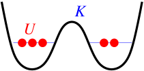
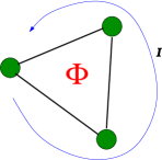
Figure 1: Illustrations of the dimer (left) and of the trimer (right) model systems. Namely, we consider $N$ bosons that are described by an $M=2$ or by an $M=3$ site BHH. The hopping frequency is $K$, and the on-site interaction is $U$. In the case of a trimer the hopping frequencies acquire phases whose sum $\Phi$ reflects the Coriolis force.

Strict condensation means to place all the bosons in a single orbital. Condensation in a momentum-orbital of the trimer is known as vortex-state. Condensation in a single site-orbital is known as self-trapped or as bright-soliton state. More generally we shall characterize the eigenstates of the BHH by a purity measure ${S\in[0,1]}$. Namely, given an eigenstate we define the reduced one-body probability matrix $\rho_{ij}=(1/N)\langle a_{j}^{{\dagger}}a_{i}\rangle$, where $a_{j}^{{\dagger}}$ are the creation operators. From that we calculate $S\equiv\mbox{trace}(\rho^{2})$. Accordingly $S=1$ implies condensation in a single orbital, also termed “coherent state”, while ${1/S\sim M}$ implies a maximally fragmented state. The purity measure $S$ reflects the one-body coherence of the many-body state: small value of $S$ implies loss of fringe visibility in an interference experiment.

The condensation of all the bosons in a single $\varphi$ orbital is an eigenstate of the BHH in the absence of interaction. The other many-body eigenstates are fragmented, meaning that several orbitals are populated. Once we turn-on the interaction, the possible scenarios are as follows: (1) The interaction stabilizes the $\varphi$ condensate. (2) As $u$ is varied a bifurcation is induced, such that the $\varphi$ condensate becomes unstable, and instead we get $M$ stable self-trapped states. (3) The interaction mixes the unperturbed $\varphi$ state with other fragmented unperturbed eigenstates. In the latter case we shall distinguish between: (3a) a quantum “Mott transition” scenario; and (3b) a semiclassical “ergodization” scenario. The last possibility is relevant if the underlying phase-space is chaotic.

In the next sections we shall discuss the stability of the $\varphi$ condensates. The outline is as follows: In section II we discuss the simplest examples for quantum quasi-stability and quantum scarring scars2 . In section III we explain that an unstable state can be semiclassically stabilized by introducing high frequency periodic driving or noise into the system. In section IV we consider the trimer system, and discuss the possibility to witness a metastable vortex-state. In the latter context we would like to clarify that the essence of “superfluidity” is the possibility to witness a metastable vortex-state. The term “metastability” rather than “stability” indicates that the eigenstate is located in an intermediate energy range. Using a simple-minded phrasing this implies that there is a possibility to observe a current-carrying stationary-state that is not decaying. The stability of such stationary state is due to the interaction. This presentation is based on csd ; csf ; ckt ; csk ; csm ; sfs ; sfc and further references therein more .

II The dimer - a minimal model for self trapping and Mott transition

The BHH of an $M$ site system is

$$\mathcal{H}\ =\ \frac{U}{2}\sum_{j=1}^{M}a_{j}^{{\dagger}}a_{j}^{{\dagger}}a_{j}a_{j}-\frac{K}{2}\sum_{j=1}^{M}\left(a_{j{+}1}^{{\dagger}}a_{j}+a_{j}^{{\dagger}}a_{j{+}1}\right)\ \ \ \$$ (3)

where $j=1\cdots M$ is the site index, $a_{j}^{{\dagger}}$ are the creation operators, and $n_{j}=a_{j}^{{\dagger}}a_{j}$ are the occupation operators. The total number of particles ${N=n_{1}+n_{2}}$ is a constant of motion hence the dynamics of an $M=2$ dimer is reduced to that of one degree-of-freedom

$$J_{z}\ \ =\ \ n\ \ =\ \ \frac{1}{2}(n_{1}-n_{2})$$ (4)

An optional way to write the dimer Hamiltonian is to say that $J_{z}$ is like the $Z$ component of a $j=N/2$ spin entity. Using this language the hopping term of the BHH merely generates Rabi rotations around the X axis. This means that the population oscillates between the two wells. The full BHH, including the interaction term, is written as follows

$$\mathcal{H}_{\text{dimer}}\ =\ U\hat{J}_{z}^{2}\ -\ K\hat{J}_{x}$$ (5)

Semiclassically the spin orientation is described by the conjugate coordinates ${(\theta,\varphi)}$, or equivalently by ${(n,\varphi)}$, where $n=(N/2)\cos(\theta)$. With each point in phase-space we can associate a spin-coherent-state $|n,\varphi\rangle$ that is obtained by SU(2) rotation of the North-pole condensation state ${(a_{1}^{{\dagger}})^{N}|\text{vaccum}\rangle}$. An arbitrary quantum state can be represented by the Husimi phase-space distribution ${\rho(\varphi,n)=|\langle n,\varphi|\psi(t)\rangle|^{2}}$. In the following paragraphs we describe how the $UJ_{z}^{2}$ term of the dimer Hamiltonian affects the Rabi rotations that are generated by $KJ_{x}$.

Bifurcation scenario.– For ${u<1}$ the dynamics that is generated by $\mathcal{H}$ is topologically the same as Rabi rotations: the phase-space trajectories around $X$ are merely deformed. This means that there are two stable fixed-points, both located on the Equator (${\theta=\pi/2}$). The ground-state fixed-point is ${\varphi=0}$, and the upper-state fixed-point is ${\varphi=\pi}$. For ${u>1}$ the ground-state fixed-point remains stable but the upper fixed-point bifurcates. Instead phase-space can support condensation in the North or in the South fixed-point. See Fig.​​ 2 for illustration. This is an example for the 2nd scenario that has been mentioned in the introduction.

Mott transition.– The dimer constitutes a minimal model also for the demonstration of the Mott transition, which is the 3rd scenario that has been mentioned in the introduction. Namely, if we increase $u$ beyond $N^{2}$ the the area of the Rabi region in phase-space becomes smaller than Planck cell. This means that the ground-state is no longer a coherent state. Rather it becomes a Fock state with 50%-50% occupation of the two wells. Semiclassically it is represented by a strip along the Equator, with uniform $\varphi$ distribution.

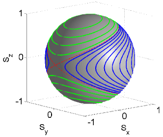
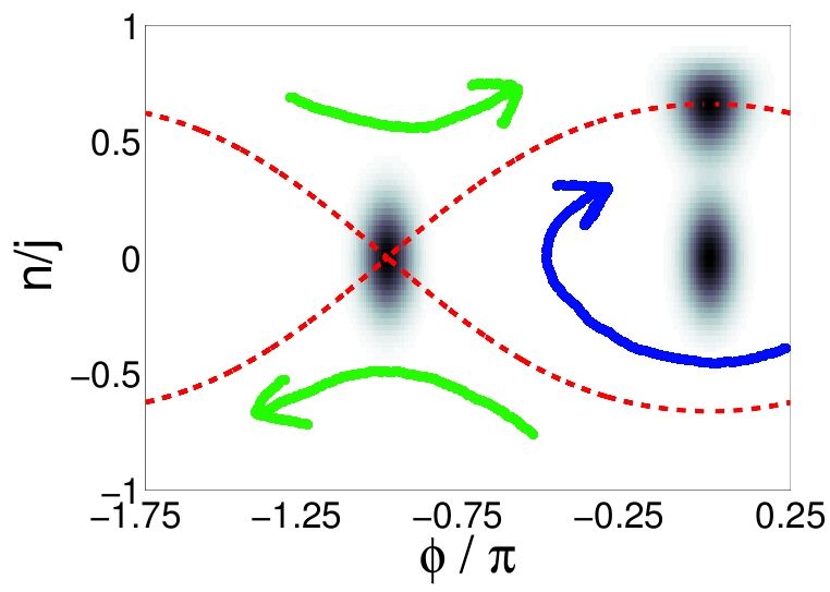
Figure 2: The dimer BHH is formally like that of a spin $j=N/2$ entity. Its spherical phase-space ${(\theta,\varphi)}$ is illustrated in the upper panel in the case ${u>1}$. It is similar to the cylindrical phase-space ${(n,\varphi)}$ of a mathematical pendulum (lower panel). We have 3 types of motion separated by a separatrix: Rabi oscillations between the two wells (blue curves); and self-trapped motion either in the left or in the right well (green curves). In the lower panel the 3 shaded Husimi distributions represent the following preparations: low-energy $\varphi{=}0$ coherent-state; separatrix-energy $\varphi{=}\pi$ coherent-state; and another coherent-state with the same energy.

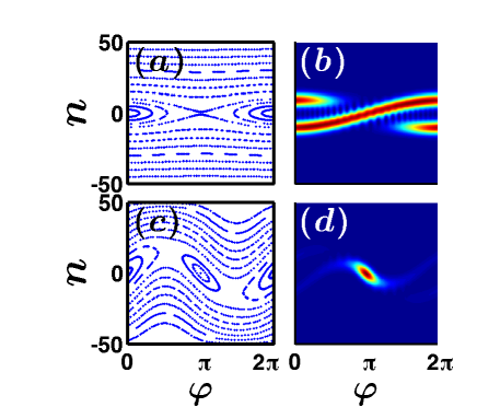
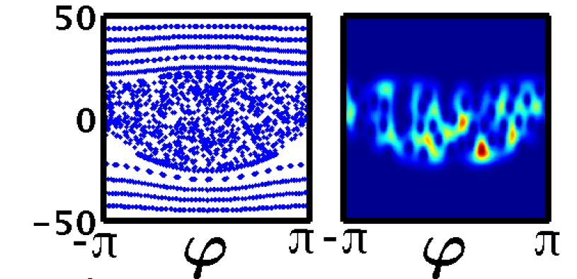
Figure 3: The dynamics of the dimer is illustrated in phase-space. For numerical details see csk . The upper panels simulate the evolution in the absence of external driving: The left panel shows the classical phase-space portrait, and the right panel provides the Husimi representation of a quantum-mechanically time-evolved $\pi$ preparation (red means high probability). The 2nd row panels show what happens if one adds high frequency periodic driving that converts the hyperbolic fixed-point into a stable elliptic fixed-point. The 3rd row panels show what happens if the driving frequency is comparable with the natural frequencies of the dynamics: one observes a chaotic sea within which the quantum state ergodizes.

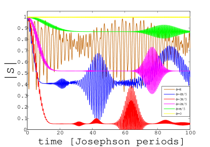
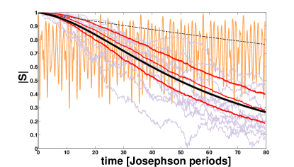
Figure 4: The length $|S|$ of the Bloch vector is a measure for one-body coherence. We follow the time evolution of a coherent state. In the upper panel each curve is for a different preparation (see text). In the lower panel the evolution of a ${\varphi=\pi}$ preparation is simulated in the presence of noise (thick black curve) and compared with noiseless evolution (orange curve). For more details see csm .

III Quasi-stability of an unstable preparation

Having figured out that for ${u>1}$ the ${\varphi=\pi}$ fixed-point is not stable, the question arises what happens if initially we condense all the bosons in the upper orbital. Semiclassically such preparation is represented by a Gaussian-like distribution at the ${\varphi=\pi}$ fixed-point, see Fig.​​ 2b. It is useful here to make a connection with the Josephson Hamiltonian. Namely, in the vicinity of the Equator Eq.​​ (5) can be approximated by

$$\mathcal{H}_{\text{Josephson}}\ \ =\ \ Un^{2}-\frac{NK}{2}\cos(\varphi)$$ (6)

where $\varphi=\varphi_{1}-\varphi_{2}$ is the conjugate phase. This is formally like the Hamiltonian of a mathematical pendulum. The ${\varphi=\pi}$ preparation is like trying to position the pendulum in the upper unstable point. Our classical intuition tells us that such state should decay exponentially. Using a phase-space picture, the wavepacket is expected to squeeze in one direction and stretch in the other (unstable) direction, along the separatrix. This is demonstrated in the upper panel of Fig.​​ 3 using the Husimi representation.

However, it turns out that the naive classical intuition with regard to the stability of the ${\varphi=\pi}$ preparation fails once longer time are considered. In the upper panel of Fig.​​ 4 we plot the time evolution of the length $S_{B}=|\bm{S}|$ of the Bloch vector for various coherent preparations

$$\bm{S}\ \ =\ \ \frac{2}{N}\left(\langle J_{x}\rangle,\langle J_{y}\rangle,\langle J_{z}\rangle\right)$$ (7)

Note that the reduced probability matrix is expressible in terms of $\bm{S}$, hence the purity measure that has been defined in the introduction is $S=(1+S_{B}^{2})/2$. The initial length ${S_{B}{=}1}$ of the Bloch vector reflects the coherence of the initial preparation. If the initial state is located along the Equator at $\varphi=0$, it remains there (stable). If it starts elsewhere it typically decays. But if it starts at $\varphi=\pi$, the motion is dominated by recurrences: it becomes quasi-periodic, hence this preparation is quasi-stable.

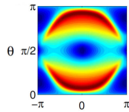
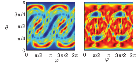
Figure 5: An image of $\text{PN}(\varphi,\theta)$. The left panel, taken from csf , is for the integrable non-driven dimer with $N{=}100$ bosons, and $u{=}2.5$. The color code goes from PN$\sim 1$ (deep blue) to PN$\sim 30$ (red). The middle and right panels are for a kicked dimer that has a mixed or a fully-chaotic phase-space, respectively. For extra details see ckt . In the latter (chaotic) case one observes scarring (blue regions) in the vicinity of the classical hyperbolic points.

In order to explain this quasi-stability we expand the initial coherent state in the basis of $\mathcal{H}$ eigenstates. Then we determine the participation number (PN) of the preparation. The PN tells how many eigenstates “participate” in the superposition. If the superposition involved all the eigenstates we would get PN$\sim N$. For a coherent-state, which is like a minimal wavepacket, the naively expected result is PN$\sim 1$ if it is located in the vicinity of a stable elliptic fixed-point, and PN$\sim\sqrt{N}$ otherwise. Fig.​​ 5 provided an image of PN for all possible coherent-preparation. The color of a given point ${(\varphi,\theta)}$ reflects the PN of a “minimal wavepacket” that is launched at that point. We see in the left panel that the PN of a $\varphi{=}\pi$ preparation is of order unity (color-coded in blue) contrary to the naive expectation. An analytic calculation using a WKB approximation csd ; csf provides the estimate PN$\sim\log(N)$. This explains the quasi-stability of the unstable fixed-point: the PN is typically small hence the motion is qusi-periodic. A huge value of $N$ is required to get the irreversible decay that would be observed in the classical limit.

The low PN of a “minimal wavepacket” that is launched at the vicinity of an hyperbolic point can be regarded as an extreme example for “quantum scarring”. The latter terms is reserved to the case where an hyperbolic point is immersed in a chaotic sea. Fig.​​ 5 provides an example for a PN calculation for a kicked dimer csk . The middle panel is for a mixed phase-space system where the low PN regions simply reflect quasi-integrable motion. The right panel is for a strongly chaotic system where the blue regions indicates the presence of a classical hyperbolic point. Strangely enough in a classical simulation the hyperbolic point cannot be detected because it has zero measure. But quantum mechanics is generous enough to acknowledge its existence. We note that in this “quantum scarring” example PN$\sim N$ for any preparation: the low PN is due to a prefactor is the quantum scarring formula, and not due to a different functional dependence on $N$.

IV Stabilization - The Kapitza and the Zeno effects

The ${\varphi=\pi}$ preparation is qusi-stable rather than stable. The question arises whether in an actual experiment it can be stabilized such that $S\sim 1$ for a long duration of time. The answer is positive. It can be stabilized by introducing hight-frequency or noisy driving. The Hamiltonian becomes

$$\mathcal{H}_{\text{total}}\ \ =\ \ \mathcal{H}\ \ +\ \ f(t)W$$ (8)

The coupling is via some $W$. In the present context we assume that the hopping amplitude $K$ is modulated, accordingly $W=J_{x}$.

By periodic driving we mean

$$f(t)\ \ =\ \ A\sin(\Omega t)$$ (9)

One should be aware that if $\Omega$ is comparable with the natural frequency of the system, we merely get chaotic dynamics as demonstrated in the lower panels of Fig.​​ 3. This means that stability is completely lost. But if we have high-frequency driving, its effect is averaged, and we get quasi-integrable motion with an effective Hamiltonian $\mathcal{H}+V^{\text{eff}}$, where

$$V^{\text{eff}}\ \ =\ \ -\frac{A^{2}}{4\Omega^{2}}\ [W,[W,\mathcal{H}]]$$ (10)

See csk for derivation. It turns out that the additional term converts the hyperbolic point into a stable elliptic point as demonstrated in the middle panels of Fig.​​ 3. This is known as the Kapitza effect. We merely generalized here the standard analysis of the canonical mathematical pendulum.

By noisy driving we mean that $f(t)$ looks like “white noise” with zero average and correlation function

$$\overline{f(t)f(t^{\prime})}\ \ =\ \ 2D\delta(t-t^{\prime})$$ (11)

Using standard elimination technique one concludes that the dynamics is described by the following Fokker-Planck equation:

$$\frac{d\rho}{dt}\ \ =\ \ -i[\mathcal{H},\rho]-D[W,[W,\rho]]$$ (12)

The analysis csm shows that the decay is described by the expression

$$S_{B}\ \ =\ \ \exp\left\{-\frac{1}{N}\left[\exp\left(8D_{w}t\right)-1\right]\right\}$$ (13)

where the radial diffusion coefficient is

$$D_{w}\ \ =\ \ \frac{w_{J}^{2}}{8D}$$ (14)

The stronger the noise, the slower the radial diffusion. Looking at Fig.​​ 4 we see that we have achieved $|S|\sim 1$ for a long duration. In the remaining paragraphs of this section we shall provide a heuristic explanation for this effect.

There is related stabilization method that comes under the misleading title “quantum Zeno effect”. The idea is to “watch” the pendulum. Due to successive “collapses” of the wavefunction the decay is slowed down. Using a standard Fermi-golden-rule analysis one deduces the expression

$$S_{B}\ \ =\ \ \exp\left\{-\frac{1}{N}8D_{w}t\right\}$$ (15)

This expression coincides with Eq.​​ (13) for very short times, and fails for longer times, as demonstrated in the lower panel of Fig.​​ 4, where it is plotted as a thin black line. What is misleading here, is the idea that the Zeno effect is a spooky quantum effect. In fact to “watch” a pendulum is formally the same as introducing noise. The effect of the noise is to stabilize the pendulum, and this would happen also if Nature were classical…

So what is the essence of the Zeno effect? The most transparent way to explain it is to use a phase-space picture. Let us regard the wavepacket as an ellipse with area ${\mathsf{A}=\pi r_{a}r_{b}}$. The effect of $\mathcal{H}$ is to squeeze it in one direction and stretch it in the other direction. Note that the area $\mathsf{A}$ is not affected (Liouville’s theorem). The effect of $f(t)J_{x}$ is to induce random rotation of its orientation. Thanks to the random rotations the stretching process is slowed down. Schematically we can write the length of the the randomly rotating major axis as

$$r(t)\ \ =\ \ \lambda_{t}\ ...\ \lambda_{2}\ \lambda_{1}\ r(0)$$ (16)

where $\lambda$ is either smaller or larger than unity depending on the orientation of the ellipse. The net effect is diffusion of $\log(r)$, leading to Eq.​​ (13). Now we can also understand what is the reason for the failure of Eq.​​ (15). The first-order treatment involves the substitution ${\lambda=1+\epsilon}$, and then the product is expanded. Hence $r(t)$ becomes a sum ${\epsilon_{t}+...+\epsilon_{2}+\epsilon_{1}}$, rather than a product of random variables, and one deduces wrongly that $r(t)$ diffuses, leading to Eq.​​ (15).

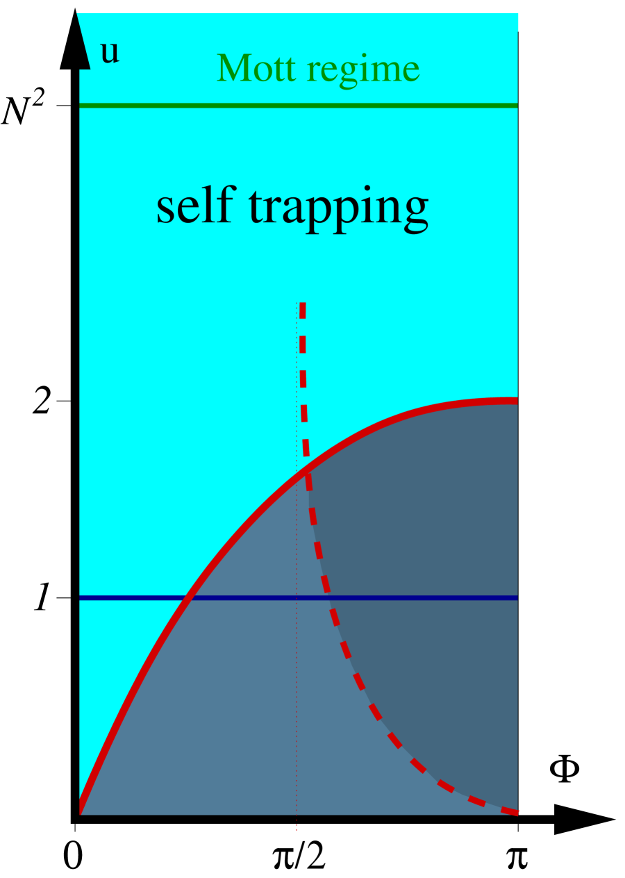
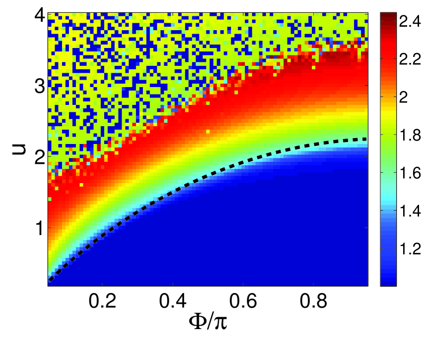
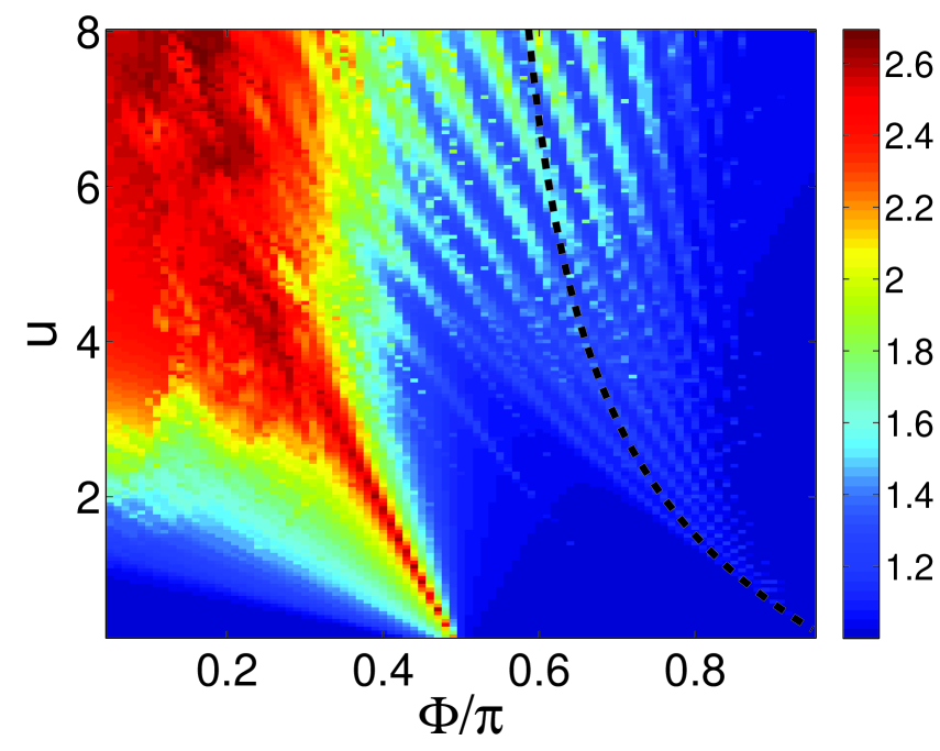
Figure 6: Regime diagram of a triangular BEC trimer with $N{=}42$ bososn, taken from sfs . The model parameters are $(\Phi,u)$. Left panel: The thick red line is the semiclassical stability border of the upper vortex-state, where it bifurcates into 3 self-trapped states. The thick dashed line is the Landau-criterion stability border of the intermediate vortex state: the expected stability region is on the right of this curve. Right panels: The inverse purity $1/S$ is imaged for the upper most eigenstate (upper panel), and for the maximal current eigenstate (lower panel). In the former case we observe an agreement with the classical stability analysis, while in the latter case we observe unexpected quasi-stability outside of the semiclassical stability region.

V The trimer - a minimal model for a superfluid circuit

The BHH of the trimer is the same as Eq.​​ (3), but for sake of generality we add in the kinetic term hopping phases that reflect the Coriolis field:

$$-\frac{K}{2}\sum_{j=1}^{M}\left(\mbox{e}^{i(\Phi/M)}a_{j{+}1}^{{\dagger}}a_{j}+\mbox{e}^{-i(\Phi/M)}a_{j}^{{\dagger}}a_{j{+}1}\right)$$ (17)

Note that this is formally like having an Aharonov-Bohm magnetic flux through the ring. The classical energy landscape of the BHH always has a lowest fixed-point that might support a vortex-state, and an upper fixed-point that might support either a vortex-state or (due to bifurcation) a set of self-trapped states. Note that the upper-state can be regarded as a ground-state of the ${U\mapsto-U}$ Hamiltonian. The $(\Phi,u)$ regime diagram of this model is displayed in the left panel of Fig.​​ 6. As in the case of the dimer we have here two familiar scenarios: With regard to the ground-state, if $u$ becomes larger than $N^{2}$ it undergoes a Mott-transition and looses its purity (green line in Fig.​​ 6). With regard to the upper-state, if $u$ crosses the solid red line, it bifurcates, and replaced by an quasi-degenerate set of 3 self-trapped states.

The inverse purity $1/S$ of the upper state is imaged as a function of $(\Phi,u)$ in the right upper panel of Fig.​​ 6. The dashed line is the classical stability border of the vortex-state beyond which we have self-trapping. Clearly the numerical results agree with the classical prediction.

The question arises whether it feasible to find a (meta)stable vortex-state, that is immersed in the “continuum”. The “continuum” is formed of states that are supported by the chaotic sea. There are two possibilities here: The traditional possibility is to have a state that is supported by a stable fixed-point in an intermediate energy; The exotic possibility is to have quasi-stability in the vicinity of an unstable fixed-point. Looking at the right lower panel of Fig.​​ 6 we find that superfluidity survives beyond the classical (Landau) border of stability. In particular we observe that superfluidity is feasible for a non-rotating device ($\Phi{=}0$), contrary to the traditional expectation that is based on the classical stability analysis. The full explanation of the superfluidity regime-diagram requires a thorough “quantum chaos” analysis of the underlying mixed phase-space structure sfc .

VI Concluding remarks

The dimer is a minimal model for demonstrating the classical instability that leads to self-trapping, and the quantum Mott transition of the ground-state. It also provides an illuminating example for quasi-stability at the vicinity of an unstable hyperbolic point. Classical stabilization is feasible by introducing high-frequency periodic driving (Kapitza effect) or noise (Zeno effect).

From topological point of view a triangular trimer is the minimal model for a superfluid circuit. Due to the extra degree of freedom this model is no longer integrable, unlike the dimer. The question arises whether such circuit can support a metastable vortex-state. This is what one call “superfluidity”. We find that a quasi-stable superfluid motion manifests itself beyond the regime that is implied by the traditional stability analysis. The full explanation of the superfluidity regime-diagram of a low-dimensional circuit requires a thorough “quantum chaos” analysis of the underlying mixed phase-space structure.

Low dimensional superfluid circuits are of current experiment interest trmexp . Periodically driven BEC circuits and the stabilization of nonequilibrium condensates is of special interest too trmdrv ; trmstb .

Acknowledgements.– The current manuscript is based on studies csd ; csf ; ckt ; csk ; csm ; sfs that have been conducted in Ben-Gurion university in collaboration with my colleague Ami Vardi. The main work has been done by Geva Arwas, Christine Khripkov, Maya Chuchem, and Erez Boukobza. The present contribution has been supported by the Israel Science Foundation (grant No.29/11).

References

- (1) O. Morsch, M. Oberthaler, Rev. Mod. Phys. 78, 179 (2006); I. Bloch, J. Dalibard, and W. Zwerger, Rev. Mod. Phys. 80, 885 (2008).
- (2) R. Franzosi, V. Penna, Phys. Rev. A 65, 013601 (2002); Phys. Rev. E 67, 046227 (2003).
- (3) M. Hiller, T. Kottos, and T. Geisel, Phys. Rev. A 79, 023621 (2009).
- (4) R. Kanamoto, H. Saito, M. Ueda, Phys. Rev. A 68, 043619 (2003),
- (5) A. Polkovnikov, E. Altman, E. Demler, B. Halperin, M.D. Lukin, Phys. Rev. A 71, 063613 (2005)
- (6) R. Kanamoto, L.D. Carr, M. Ueda, Phys. Rev. Lett. 100, 060401 (2008)
- (7) O. Fialko, M.-C. Delattre, J. Brand, A.R. Kolovsky, Phys. Rev. Lett. 108, 250402 (2012)
- (8) P. Ghosh, F. Sols, Phys. Rev. A 77, 033609 (2008)
- (9) L. Kaplan, E.J. Heller, Phys. Rev. E 59, 6609 (1999).
- (10) M. Chuchem, K. Smith-Mannschott, M. Hiller, T. Kottos, A. Vardi, D. Cohen, Phys. Rev. A 82, 053617 (2010).
- (11) C. Khripkov, D. Cohen, A. Vardi, J. Phys. A 46, 165304 (2013).
- (12) C. Khripkov, D. Cohen, A. Vardi, Phys. Rev. E 87, 012910 (2013).
- (13) E. Boukobza, M.G. Moore, D. Cohen, A. Vardi, Phys. Rev. Lett. 104, 240402 (2010).
- (14) C. Khripkov, A. Vardi, D. Cohen, Phys. Rev. A 85, 053632 (2012); Eur. Phys. J. Special Topics 217, 215 (2013).
- (15) G. Arwas, A. Vardi, D. Cohen, Phys. Rev. A (2014).
- (16) G. Arwas, A. Vardi, D. Cohen (in preparation).
- (17) For a more comprehensive list of references see csd ; csf ; ckt ; csk ; csm ; sfs , in particular csd (dimer) and sfs (trimer).
- (18) L. Amico, D. Aghamalyan, F. Auksztol,H. Crepaz, R. Dumke, L.C. Kwek, Sci. Rep. 4, 4298 (2014).
- (19) M. Heimsoth, C.E. Creffield, L.D. Carr, F. Sols, New Journal of Physics 14 075023 (2012)
- (20) B. Gertjerenken, M. Holthau, arXiv:1410.8008