Reduced-Order Modeling Of Hidden Dynamics

Abstract

The objective of this paper is to investigate how noisy and incomplete observations can be integrated in the process of building a reduced-order model. This problematic arises in many scientific domains where there exists a need for accurate low-order descriptions of highly-complex phenomena, which can not be directly and/or deterministically observed. Within this context, the paper proposes a probabilistic framework for the construction of “POD-Galerkin” reduced-order models. Assuming a hidden Markov chain, the inference integrates the uncertainty of the hidden states relying on their posterior distribution. Simulations show the benefits obtained by exploiting the proposed framework.

Index Terms—  Reduced-order modeling, POD-Galerkin projection, hidden Markov model, uncertainty, optic-flow.

1 Introduction

In many fields of Sciences, one is interested in studying the spatio-temporal evolution of a state variable characterized by a differential equation. Numerical discretization in space and time leads to a high dimensional system of equations of the form:

$$\left\{\begin{aligned} &x_{t+1}=f_{t}(x_{t},\theta_{t}),\\ &x_{1}=\theta_{1},\end{aligned}\right.\vspace{-0.25cm}$$ (1)

where $x_{t}\in\mathds{R}^{n}$ is the spatial discretization of the state variable at time $t$, $f_{t}:\mathds{R}^{n}\times\mathds{R}^{p_{t}}\to\mathds{R}^{n}$ and $\theta_{t}\in\mathds{R}^{p_{t}}$ denotes some parameters. As a few examples of systems obeying this type of constraints, one can mention the wave equation characterizing the propagation of sound [1], the Navier-Stokes equations describing fluid evolution [2] or the Maxwell’s equations governing the realm of electromagnetism [1]. Because (1) may correspond to a very high-dimensional system in some applications, computing a trajectory $\{x_{t}\}_{t}$ given some parameters $\{\theta_{t}\}_{t}$ may lead to unacceptable computational burdens.

To deal with this computational bottleneck, the concept of “reduced-order models” (ROMs) has been introduced in many communities dealing with high-dimensional systems. The idea of ROMs is fairly simple: one wishes to find a system involving a small number of degrees of freedom (typically ten to one hundred) while allowing for a reasonable characterization of the state of the high-dimensional system, in a certain range of operating regimes. Due to their paramount practical importance, the construction of ROMs has a fairly long history in the community of experimental physics and geophysics, beginning with the pioneering works of Lorenz in the 60’s [3, 4, 5]. Among others, one can mention Hankel norm approximations [6], principal orthogonal decomposition combined with Galerkin projections (POD-Galerkin) [7], principal oscillating patterns or principal interacting patterns [8]. We refer the reader to the book by Antoulas for a review [9].

The set of operating regimes to be reproduced by a ROM is of the form

$$\mathcal{X}\triangleq\{{\mathbf{x}}\triangleq(x_{1}\cdots x_{T}):{\mathbf{x}}\mbox{ obeys \eqref{eq:model_init} with $\{\theta_{t}\}_{t=1}^{T}\in\mathcal{R}$ }\},$$

where $\mathcal{R}\subseteq\mathds{R}^{p_{1}}\times\cdots\times\mathds{R}^{p_{T}}$. In words, the set of regimes $\cal{X}$ is defined by the set $\mathcal{R}$ of admissible parameters, which determines state trajectories through recursion (1). The set $\mathcal{X}$ may either be known perfectly or only partially. In the first situation, the construction of a ROM can rely on the perfect characterization of a representative set of trajectories, as soon as recursion (1) can be computed for the known regimes, see e.g., [10]. Building a ROM in the second situation is more subtle: representative trajectories can not be computed directly by (1) since there exists an uncertainty on the regimes of interest. For example, in fluid mechanics, the initial and the boundary conditions, defining the evolution of the fluid, are rarely perfectly known. A third situation, which is even more dramatic, emerges when recursion (1) is intractable due to a prohibitive computational burden. This typically happens in climate studies, where it is inconceivable to use high-dimensional numerical simulations for determining global warming scenarios.

A useful ingredient in these uncertain and/or intractable contexts is to incorporate partial observations of $x_{t}$’s in the process of ROM construction. For example, in geophysics, satellites daily provide a huge quantity of observations on the ocean or the atmosphere evolution. In the literature, a common strategy consists in substituting the representative trajectories (intractable to compute in these cases) by a set of observations representative of the regimes [11, 12, 13]. Nevertheless, this straightforward approach is in most experiments flawed. It ignores that observations may be incomplete and affected by noise which may dramatically impact the ROM.

In this paper, we propose a new model-reduction technique which: (i) accounts for the uncertainties in the system to reduce; (ii) exploits observations in the reduction process while taking into account their imperfect nature. We focus on the family of ROMs based on POD-Galerkin projection and recast the latter within a probabilistic framework. In a nutshell, our approach is based on a probabilistic characterization of the uncertainties of the high-dimensional system given the data, and the exploitation of this posterior information in the reduction process. We illustrate the proposed approach by the reduction of a system of 2D Navier-Stokes equations.

2 A Posteriori Inference Problem

2.1 Surrogate Prior and Observation Models

Our first step will consist in defining a high-dimensional probabilistic model gathering the uncertainty on the state of the system. Because we are assuming that there are some uncertainties in the set of admissible parameter $\mathcal{R}$ (i.e., the set of operating regimes $\mathcal{X}$), we will suppose that each $\theta_{t}$ in (1) is the realization of a random variable $\Theta_{t}$ distributed according to a probability measure $\kappa_{t}$ of support $\mathcal{R}$. This implies that $x_{t}$ is seen as a realization of a random variable $X_{t}$ distributed according to some probability measure $\nu_{t}$ of support $\mathcal{X}$.

As mentioned previously, the problem is that we are unaware of $\mathcal{X}$, since we do not have a perfect knowledge of $\mathcal{R}$. Assume now we know a measure $\eta_{t}$ dominating $\nu_{t}$, that is for any element $A$ of the Borel sets in $\mathds{R}^{n}$, $\eta_{t}(A)=0$ implies $\nu_{t}(A)=0$. Since $\nu_{t}$ is unknown, we will use $\eta_{t}$ as a surrogate measure on the unknown operating regimes. Because of the domination relation, state trajectories belonging to the unknown set $\mathcal{X}$ will have a non-zero probability. We further assume that the $\eta_{t}$’s are characterized by a probabilistic model of the form:

$$\left\{\begin{aligned} &X_{t}=b_{t}(X_{t-1})+V_{t},\quad V_{t}\sim\zeta^{v}_{t}(dv_{t}),\\ &X_{1}\sim\eta_{1}(dx_{1}),\end{aligned}\right.$$ (2)

where we have introduced some operator $b_{t}:\mathds{R}^{n}\to\mathds{R}^{n}$ and where the $V_{t}$’s are mutually independent random variables of realization $v_{t}\in\mathds{R}^{n}$ and of probability measure $\zeta^{v}_{t}$. The definition of (LABEL:eq:recOrginalNon) usually stems from the inclusion of some knowledge on the physics and the nature of the uncertainties. Indeed, there often exist approximated probabilistic characterizations of deterministic chaotic systems, see e.g., [14, 15, 16, 17] for turbulent systems.

On top of a prior information $\eta_{t}$ on the ${X}_{t}$, we assume that we have at our disposal a set of $M$ observations on the states of the system, say $\{Y^{i}_{t}\}_{i=1}^{M}$. For a sequence of $T$ state variables observed $M$ times, we define the random matrices $\mathbf{{X}}\triangleq(X_{1}\cdots X_{T})$ and $\mathbf{{Y}}\triangleq(Y^{1}_{1}\cdots Y^{1}_{T}\,Y^{2}_{1}\cdots Y^{M}_{T})$ of realizations ${\mathbf{x}}=(x_{1}\cdots x_{T})~{}\in~{}\mathds{R}^{n\times T}$ and $\mathbf{y}=(y^{1}_{1}\cdots y^{1}_{T}\,y^{2}_{1}\cdots y^{M}_{T})\in\mathds{R}^{m\times TM}$. Assume $X_{t}$’s and $Y^{i}_{t}$’s satisfy

$$Y^{i}_{t}=h_{t}(X_{t})+W_{t},\quad W_{t}\sim\zeta^{w}_{t}(dw_{t}),$$ (3)

where we have introduced some operator ${h}_{t}:\mathds{R}^{n}\to\mathds{R}^{m}$ and where the $W_{t}$’s are mutually independent noises of realization $w_{t}\in\mathds{R}^{m}$ and of probability measure $\zeta^{w}_{t}$. Given this set of observations, one can hope to remove certain uncertainties on the system regime, the final goal being to include this information in the model reduction process. In the following, we will be interested in Bayesian estimators relying on the joint posterior measure of $\mathbf{X}$ given some observation $\mathbf{Y}=\mathbf{y}$, say $\mu$. The posterior measure will be associated to the hidden Markov model (HMM) defined by (LABEL:eq:recOrginalNon) - (3). For HMMs, the posterior admits the factorization [18]

$$\mu(d{\mathbf{x}},\mathbf{y})=\frac{g({\mathbf{x}},\mathbf{y})\eta(d{\mathbf{x}})}{\langle g(\cdot,\mathbf{y}),\eta\rangle},$$ (4)

with the prior $\eta(d{\mathbf{x}})\triangleq\eta_{1}(dx_{1})\prod_{t=2}^{T}\zeta^{v}_{t}(dx_{t}-b_{t}(x_{t-1})),$ and the likelihood $g({\mathbf{x}},d\mathbf{y})\triangleq\prod_{t=1,i=1}^{T,M}\zeta^{w}_{t}(dy^{i}_{t}-h_{t}(x_{t}))$, where the expectation for any integrable function $\varphi$ is

$$\langle\eta,\varphi\rangle\triangleq\int_{\mathds{R}^{n\times T}}\eta(d{\mathbf{x}})\varphi(d{\mathbf{x}}).$$

Let us remark that, under specific conditions, a Bayesian estimator is asymptotically efficient [19]. In other words, for $M$ sufficiently large, the effect of the prior probability (LABEL:eq:recOrginalNon) on the posterior is negligible.

2.2 Uncertainty-Aware POD-Galerkin Projection

The low-rank approximation called Galerkin projection of the dynamics (1) is obtained by projecting $x_{t}$’s onto a subspace spanned by the columns of some matrix $\mathbf{u}\in\mathds{R}^{n\times k}$ where $k<n$ [7]. More precisely, it consists in a recursion

$$\left\{\begin{aligned} &z_{t}=\mathbf{u}^{*}{f}_{t}(\mathbf{u}z_{t-1},\theta_{t-1}),\\ &z_{1}=\mathbf{u}^{*}\theta_{1},\end{aligned}\right.\vspace{-0.25cm}$$ (5)

implying a sequence of $k$-dimensional variables $\{z_{t}\in\mathds{R}^{k}\}_{t}$, where the exponent ^∗ denotes the conjugate transpose. Because $k<n$, system (5) is usually tractable. Once recursion (5) has been evaluated, an approximation of state $x_{t}$ can be obtained by a matrix-vector multiplication $\mathbf{u}z_{t}$.

There exist several criteria in the literature to choose matrix $\mathbf{u}$ [9]. The POD-Galerkin approximation infers matrix $\mathbf{u}$ by minimizing the cost $\phi:\mathds{R}^{n\times T}\times\mathds{R}^{n\times k}\to\mathds{R}_{+}$

$$\phi({\mathbf{x}},\mathbf{u})\triangleq\parallel{\mathbf{x}}-\mathbf{u}\mathbf{u}^{*}{\mathbf{x}}\parallel^{2}_{F},$$ (6)

over the set of unitary matrices $\mathcal{U}=\{\mathbf{u}\in\mathds{R}^{n\times k}|\mathbf{u}^{*}\mathbf{u}=\mathbf{i}_{k}\},$ where $\mathbf{i}_{k}$ denotes the $k$-dimensional identity matrix.

In the context of our probabilistic modeling, ${\mathbf{x}}$ is a realization of some random variable governed by (LABEL:eq:recOrginalNon) which is indirectly observed through (3). The uncertainty on the state ${\mathbf{x}}$ given some observation $\mathbf{Y}=\mathbf{y}$ is quantified by the posterior (4). Using this information, we define the inference of matrix $\mathbf{u}$ for POD-Galerkin projection as the solution of

$$\operatorname*{arg\,min}_{\mathbf{u}\in\mathcal{U}}\langle\mu(\cdot,\mathbf{y}),\phi(\cdot,\mathbf{u})\rangle.\vspace{-0.15cm}$$ (7)

We discuss the resolution of this problem in the next section.

3 Computational Considerations

3.1 Solution in Terms of Posterior Expectation

While being non-convex, problem (7) admits a closed-form solution in terms of posterior expectation. Let $\{\sigma_{j}\}_{j=1}^{n}$ and $\{\hat{u}_{j}\}_{j=1}^{n}$ respectively denote the eigenvalues and eigenvectors of

$$\langle\mu(d{\mathbf{x}},\mathbf{y}),{\mathbf{x}}{\mathbf{x}}^{*}\rangle,$$ (8)

with $\sigma_{j}\geq\sigma_{j+1}$. For any $k$-dimensional unitary basis $\mathbf{u}$, it is straightforward to deduce that the expected cost in (7) admits the lower bound $\sum_{j=k+1}^{n}\sigma_{j}\leq\langle\mu(\cdot,\mathbf{y}),\phi(\cdot,{\mathbf{u}})\rangle,$ and that this bound is reached for the matrix $\hat{\mathbf{u}}$ whose columns are the eigenvectors $\{\hat{u}_{j}\}_{j=1}^{k}$ associated to the $k$ largest eigenvalues $\{\sigma_{j}\}_{j=1}^{k}$, see [20, 21]. Expectation (8) can be decomposed as

$$\langle\mu(d{\mathbf{x}},\mathbf{y}),{\mathbf{x}}{\mathbf{x}}^{*}\rangle=\sum_{t=1}^{T}\mathbf{p}_{t}+\bar{x}_{t}(\mathbf{y})\bar{x}_{t}^{*}(\mathbf{y}).$$ (9)

where $\bar{x}_{t}(\mathbf{y})\in\mathds{R}^{n}$ and $\mathbf{p}_{t}\in\mathds{R}^{n\times n}$ are the a posteriori mean and covariance of $x_{t}$ given $\mathbf{y}$. In the particular case of Gaussian linear or finite state HMMs, the posterior mean and covariance are explicitly given by Kalman recursions or by the Baum-Welsh re-estimation formulae [22]. In the general case, expectations with respect to the posterior measure (4) do not admit closed-form expressions. Nevertheless, sequential Monte-Carlo methods provide asymptotically consistent estimators [18].

We highlight the relevance of the proposed approach by a comparison with the standard snapshot method [10]. This method consists in computing $\mathbf{\hat{u}}$ as the $k$ first eigenvectors of

$$\sum_{t=1}^{T}\hat{x}_{t}(\mathbf{y})\hat{x}_{t}^{*}(\mathbf{y}),$$ (10)

where $\hat{x}_{t}(\mathbf{y})$ denotes some estimate of the state $x_{t}$ given observations $\mathbf{y}$. Consequently, the snapshot method ignores directions where the covariance of the estimation error is large due to incomplete or noisy observations. In particular, for the minimum mean square error estimator $\hat{x}_{t}(\mathbf{y})=\bar{x}_{t}(\mathbf{y})$, it neglects the influence of $\mathbf{p}_{t}$ in (9). With the proposed approach, the columns of $\hat{\mathbf{u}}$ will also be chosen in the directions in which the eigenvalues of $\mathbf{p}_{t}$ are large, i.e., directions where some uncertainty remains a posteriori.

3.2 Complexity Issues and Krylov Approximations

Assuming we can compute matrix (8), which is usually full rank, the complexity necessary to solve exactly the eigenvalue problem scales as $\mathcal{O}(n^{2}k)$ [23]. Since the goal is to lower the problem dimension, one is inevitably faced to a prohibitive dimensionality $n$. We choose to resort to Krylov subspace approximations [9]. In a nutshell, an approximation in Krylov subspaces enables to represent a large matrix by some approximated singular value decomposition, where the $k$ eigenvectors associated to the largest eigenvalues are approximated relying on the Arnoldi iteration method [24]. The method complexity scales as $\mathcal{O}(k^{2}n)$, i.e., presents the great advantage to be linear with respect to the state variable dimension. It is comparable to the complexity $\mathcal{O}(T(T^{2}+n))$ required by the diagonalisation of matrix (10) of rank $T$ and by the matrix-vector multiplications in the snapshot method.

4 Numerical Example

4.1 Reduction of 2D Navier-Stokes Equations

4.1.1 2D Turbulence Model

We illustrate the proposed methodology within the context of reducing a 2D model of turbulence from a video depicting the evolution of a scalar field transported by the flow. As described in [25], the high-dimensional model (1) is here a quadratic function with respect to a spatial discretization of the flow velocity $x_{t}\in\mathds{R}^{n}$

$$f_{t}(x_{t},\theta_{t})=\mathbf{c}^{*}(\mathbf{i}_{n}+\alpha\boldsymbol{\ell}-x_{t}^{*}\mathbf{r})\mathbf{c}x_{t}+\theta_{t},$$ (11)

where $\alpha\in\mathds{R}^{+}$ denotes a dissipation coefficient and where matrices $\boldsymbol{\ell}\in\mathds{R}^{m\times m}$, $\mathbf{c}\in\mathds{R}^{m\times n}$ and $\mathbf{r}\in\mathds{R}^{n\times m}$ with $n=2m$ are discrete versions of respectively the Laplacian, the curl and the spatial gradient operators. Variable $\theta_{t}\in\mathds{R}^{n}$ accounts for some forcing. The observation model relates the flow velocity $x_{t}$ to the variation $y_{t}\in\mathds{R}^{m}$ of the intensity of a scalar field conveyed by the flow. It takes the form of (3) with a zero-mean uncorrelated Gaussian noise $W_{t}$ of variance $\sigma^{2}$ and with a linear function

$$h_{t}(x_{t})=\mathbf{h}_{t}x_{t}+\xi_{t},$$ (12)

for some matrix $\mathbf{h}_{t}\in\mathds{R}^{m\times n}$ and vector $\xi_{t}\in\mathds{R}^{m}$, see [25]. We use the high-dimensional model to produce one sequence of 2D motion field $\{x_{t}\}_{t=1}^{T}\in\mathcal{X}$ for a given operating regime $\{\theta_{t}\}_{t=1}^{T}\in\mathcal{R}$ and one sequence ($M=1$) of scalar fields of intensity variations $y^{1}_{t}$’s. In the sequel, we denote these sequences as $({\mathbf{x}}^{dns},\mathbf{y}^{dns})\in\mathds{R}^{n\times T}\times\mathds{R}^{m\times T}$.

4.1.2 Optic-Flow Posterior

As suggested in the literature of optic-flow and turbulence modeling, we will rely on a degenerated case of the surrogate prior (LABEL:eq:recOrginalNon) where $b_{t}(X_{t-1})$ vanishes. Moreover, we assume that $V_{t}$’s are zero-mean Gaussian random fields. Such priors are commonly used in computer vision [26], in fluid mechanics [16], or in geophysics [17] to describe the correlated structure of motion fields. These priors fulfill the domination condition. They are usually degenerated and defined by an inverse covariance $\mathbf{q}_{t}\in\mathds{R}^{n\times n}$ of rank lower than $n$. The latter matrix implements typically some local regularity constraints, e.g., finite difference approximation of spatial gradients [26], or some self-similar constraints and long-range dependency proper to turbulent flows [16, 17]. In this linear Gaussian setting, we obtain the posterior mean and covariance

$$\left\{\begin{aligned} &\bar{x}_{t}(\mathbf{y})=\sigma^{-2}\mathbf{p}_{t}\mathbf{h}_{t}^{*}(y^{1}_{t}-\xi_{t}),\\ &\mathbf{p}_{t}=\sigma^{2}(\mathbf{h}_{t}^{*}\mathbf{h}_{t}+\sigma^{2}\mathbf{q}_{t})^{-1}.\vspace{-0.25cm}\end{aligned}\right.\vspace{-0.25cm}$$ (13)

4.2 Experimental Setting, Results and Discussion

Our simulations use a sample composed of $T=50$ consecutive states and images of size $m=2^{7}\times 2^{7}$. We evaluate two different choices for $\mathbf{q}_{t}$: the standard gradient model [26] and the self-similar model proposed in [17]. The inversion of the $n\times n$ matrices appearing in (13) are approximated within a linear complexity in a $10$-dimensional Krylov subspace. The $k=50$ first eigenvectors of (9) composing the columns of the minimizer $\hat{\mathbf{u}}$ of (7) are then approximated using a Krylov subspace of dimension $100$.

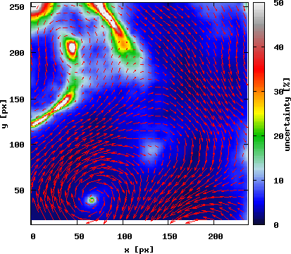
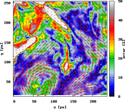
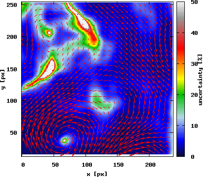
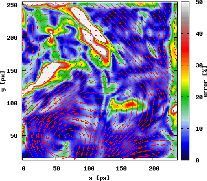
Fig. 1: Left: mean of the posterior bi-variate vector (arrows) and Frobenius norm of its covariance (color map) at each point of the pixel grid for $t=25$ . Results for standard [26] (above) or self-similar prior [17] (below). Right: ground truth bi-variate vector (arrows) and error (14) (color map) for the standard (above) or self-similar (below) prior.

Fig. 1 illustrates the Gaussian posterior distribution of a turbulent flow obtained by optic-flow modeling, using Krylov approximation. The local posterior covariance (in fact the Frobenius norm of the local $2\times 2$ covariance matrix) can be compared to the normalized squared $\ell_{2}$-norm error between the realization ${\mathbf{x}}^{dns}\triangleq(x_{1}^{dns}\cdots x_{T}^{dns})$ and the estimated posterior mean, i.e.,

$${\|(x^{dns}_{t})_{s}-(\bar{x}_{t}(\mathbf{y}^{dns}))_{s}\|^{2}_{2}}/{\|(x^{dns}_{t})_{s}\|^{2}_{2}},$$ (14)

where the subscript $s$ denotes the vector (bi-variate) component related to the $s$-th pixel of the image grid. A visual inspection of the different maps shows that : 1) the region with high variances correspond to areas characterized by large errors (14); 2) conversely, in the case of the self-similar prior, most regions with large errors (14) correspond to areas with high variances; besides, the error is globally lower for the self-similar prior. The first observation serves as a clear evidence of the relevance of integrating the posterior distribution in the ROM building process. The second remark shows the importance of using good prior surrogates.

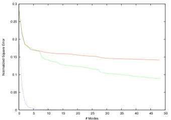
Fig. 2: Evolution of the normalized error (15) with respect to the dimension $k$ of the inferred reduced basis with the state-of-the-art snapshot method [10] (red solid line), the proposed method (green dashed line) and using directly the ground truth (blue dotted line).

The plot of Fig. 2 shows the evolution of the normalized square reconstruction error induced by low-rank approximation of the true flow, i.e.,

$${\|{\mathbf{x}}^{dns}-\hat{\mathbf{u}}\hat{\mathbf{u}}^{*}{\mathbf{x}}^{dns}\|^{2}_{F}}/{\|{\mathbf{x}}^{dns}\|^{2}_{F}},$$ (15)

with respect to the number of columns $k$ of matrix $\hat{\mathbf{u}}$, the solution of (7) using the prior model in [26]. We evaluate the snapshot method and the proposed posterior reduced-order modeling. Moreover, the figure also includes the plot of the error (15) obtained with a reduced basis $\hat{\mathbf{u}}$ inferred when ${\mathbf{x}}^{dns}$ is directly available without uncertainty. We note that in principle, in order to evaluate the error induced by the ROM, the orthogonal complement ${\|\hat{\mathbf{u}}\hat{\mathbf{u}}^{*}{\mathbf{x}}^{dns}-\hat{\mathbf{u}}\mathbf{z}\|^{2}_{F}}/{\|{\mathbf{x}}^{dns}\|^{2}_{F}}$ should be added to error (15), with $\mathbf{z}=(z_{1}\cdots z_{T})$ computed from (5) using $x_{1}^{dns}$ [7]. Unfortunately, [25] does not provide the detailed implementation of function (11).

We immediately remark that including uncertainty in the process of reduced-order modeling induces a clear gain in accuracy. The error reduction is more than 30 $\%$. It is nevertheless modest in comparison to the gain obtained by ROM directly inferred from ground truth. In the light of comments of Fig. 1, we believe that this error gap may be significantly reduced by using more relevant priors, such as those proposed in [16, 17]. This is the topic of ongoing research.

5 Conclusion

We have proposed a methodology for building ROMs which integrates the high-dimensional system uncertainties. It relies on the computation of an a posteriori measure. This information reveals directions where uncertainty on the states remain high and where observations were insufficient to solve the regime ambiguities. We show how to integrate this a posteriori information in the construction of ROMs based on POD-Galerkin projections. Numerical experiments, taking place in the context of 2D Navier-Stokes equations, show that the proposed probabilistic framework enables to lower significantly the reconstruction error in comparison to the standard “POD-snapshot” method.

References

- [1] E. Godlewski and P.A. Raviart, Numerical Approximation of Hyperbolic Systems of Conservation Laws, Number n 118 in Applied Mathematical Sciences. Springer, 1996.
- [2] L. Quartapelle, Numerical Solution of the Incompressible Navier-Stokes Equations, International Series of Numerical Mathematics. Birkhäuser Basel, 2013.
- [3] E.N. Lorenz, “Empirical orthogonal functions and statistical weather prediction,” Scientific Report 1, Statistical Forecasting Project, MIT, Cambridge, MA, 1956.
- [4] E.N. Lorenz, “Maximum simplification of the dynamic equations,” Tellus, vol. 12, no. 3, pp. 243–254, 1960.
- [5] E. N. Lorenz, “Deterministic Nonperiodic Flow.,” Journal of Atmospheric Sciences, vol. 20, pp. 130–148, Mar. 1963.
- [6] M. Green and D.J.N. Limebeer, Linear Robust Control, Dover Books on Electrical Engineering. Dover Publications, Incorporated, 2012.
- [7] C. Homescu, L. R. Petzold, and R. Serban, “Error estimation for reduced-order models of dynamical systems,” SIAM Review, vol. 49, no. 2, pp. 277–299, 2007.
- [8] K. Hasselmann, “Pips and pops: The reduction of complex dynamical systems using principal interaction and oscillation patterns,” Journal of Geophysical Research: Atmospheres, vol. 93, no. D9, pp. 11015–11021, 1988.
- [9] A.C. Antoulas, Approximation of Large-scale Dynamical Systems, Advances in Design and Control. Society for Industrial and Applied Mathematics, 2005.
- [10] L. Sirovich, “Turbulence and the dynamics of coherent structures.,” Quarterly of Applied Mathematics, vol. 45, pp. 561–571, Oct. 1987.
- [11] D. Moreno, A. Krothapalli, M. B. Alkislar, and L. M. Lourenco, “Low-dimensional model of a supersonic rectangular jet,” Phys Rev E (69: 026304), pp. 1–12, 2004.
- [12] J. D’Adamo, N. Papadakis, E. Memin, and G. Artana, “Variational assimilation of pod low-order dynamical systems,” Journal of Turbulence, vol. 8, no. 9, pp. 1–22, 2007.
- [13] H. von Storch and F.W. Zwiers, Statistical Analysis in Climate Research, Cambridge University Press, 2001.
- [14] R. Robert and V. Vargas, “Hydrodynamic turbulence and intermittent random fields,” Communications in Mathematical Physics, vol. 284, pp. 649–673, 2008.
- [15] L. Chevillard, R. Robert, and V. Vargas, “A stochastic representation of the local structure of turbulence,” EPL (Europhysics Letters), vol. 89, no. 5, pp. 54002, 2010.
- [16] P. Heas, F. Lavancier, and S. Kadri Harouna, “Self-similar prior and wavelet bases for hidden incompressible turbulent motion,” SIAM Journal on Imaging Sciences, vol. 7, pp. 1171–1209, 2014.
- [17] P. Heas, C Herzet, E. Memin, Heitz D., and P.D. Mininni, “Bayesian estimation of turbulent motion,” IEEE transactions on Pattern Analysis And Machine Intelligence, vol. 35, no. 6, pp. 1343–56, 2013.
- [18] P.D. Moral, Feynman-Kac Formulae: Genealogical and Interacting Particle Systems with Applications, Probability and Its Applications. Springer New York, 2012.
- [19] E.L. Lehmann and G. Casella, Theory of Point Estimation, Springer Texts in Statistics. Springer New York, 2003.
- [20] R.M. Johnson, “On a theorem stated by Eckart and Young,” Psychometrika, vol. 28, no. 3, pp. 259–263, 1963.
- [21] R. A. Horn and C. R Johnson, Matrix analysis, Cambridge university press, 2012.
- [22] M. Briers, A. Doucet, and S. Maskell, “Smoothing algorithms for state–space models,” Annals of the Institute of Statistical Mathematics, vol. 62, no. 1, pp. 61–89, 2010.
- [23] G.H. Golub and C.F. Van Loan, Matrix Computations, Johns Hopkins Studies in the Mathematical Sciences. Johns Hopkins University Press, 1996.
- [24] W. E. Arnoldi, “The principle of minimized iteration in the solution of the matrix eigenvalue problem,” Quarterly of Applied Mathematics, vol. 9, pp. 17–29, 1951.
- [25] J. Carlier and B. Wieneke, “Report 1 on production and diffusion of fluid mechanics images and data,” Fluid project deliverable 1.2., 2005.
- [26] B. Horn and B. Schunck, “Determining optical flow,” Artificial Intelligence, vol. 17, pp. 185–203, 1981.