Quantum oscillations in a bilayer with broken mirror symmetry: a minimal model for YBa₂Cu₃O_6+δ

Abstract

Using an exact numerical solution and semiclassical analysis, we investigate quantum oscillations (QOs) in a model of a bilayer system with an anisotropic (elliptical) electron pocket in each plane. Key features of QO experiments in the high temperature superconducting cuprate YBCO can be reproduced by such a model, in particular the pattern of oscillation frequencies (which reflect “magnetic breakdown” between the two pockets) and the polar and azimuthal angular dependence of the oscillation amplitudes. However, the requisite magnetic breakdown is possible only under the assumption that the horizontal mirror plane symmetry is spontaneously broken and that the bilayer tunneling, $t_{\perp}$, is substantially renormalized from its ‘bare’ value. Under the assumption that $t_{\perp}=\tilde{Z}t_{\perp}^{(0)}$, where $\tilde{Z}$ is a measure of the quasiparticle weight, this suggests that $\tilde{Z}\lesssim 1/20$. Detailed comparisons with new YBa₂Cu₃O_6.58 QO data, taken over a very broad range of magnetic field, confirm specific predictions made by the breakdown scenario.

Quantum oscillations (QOs) are a spectacular consequence of the presence of a Fermi surface. Their observation in the high $T_{c}$ cuprate superconductorsDoiron-Leyraud et al. (2007); LeBoeuf et al. (2007); Bangura et al. (2008); Yelland et al. (2008); Vignolle et al. (2008); Audouard et al. (2009); Sebastian et al. (2010); Singleton et al. (2010); Ramshaw et al. (2011); Sebastian et al. (2012a, b); Barišić et al. (2013); Sebastian et al. (2014); Sebastian and Proust (2015); Ramshaw et al. (2015) combined with recent observations of charge density wave correlationsTranquada et al. (1994, 1995); Fujita et al. (2004); Howald et al. (2003); Hoffman et al. (2002); Hanaguri et al. (2004); Fink et al. (2009); Laliberté et al. (2011); Chang et al. (2012); Ghiringhelli et al. (2012); Achkar et al. (2012); Doiron-Leyraud et al. (2013); LeBoeuf et al. (2013); He et al. (2014); Tabis et al. (2014); Forgan et al. (2015), have led to a compelling view of the non-superconducting “normal” state of the underdoped cuprates at high fields, $H>H_{c}$, and low temperatures, $T\ll T_{c}$. In this regime, small electron-like Fermi pockets arise from reconstruction of a larger hole-like Fermi surface presumably due to translation symmetry breaking in the form of bidirectional charge-density-wave (CDW) orderChakravarty et al. (2001); Millis and Norman (2007); Harrison and Sebastian (2011); Eun et al. (2012); Harrison and Sebastian (2012); Lee (2014); Allais et al. (2014); Wang and Chubukov (2014); Maharaj et al. (2014); Russo and Chakravarty (2015); Briffa et al. (2015); Harrison et al. (2015).

However, to date, no theory of Fermi-surface reconstruction by a simple CDW can simultaneously account for the Fermi pockets and the relatively small magnitude of the measured specific heat,Yao et al. (2011); Riggs et al. (2011) which presumably reflects the persistence a pseudo-gap that removes other portions of the original (large) Fermi surface. Thus, rather than trying to infer the origin of the Fermi pockets, we explore a generic model of a single bilayer split pocket to elucidate general features that can most easily account for the salient features of the QOs.

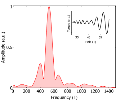
Figure 1: Typical Fourier transform of QOs of the magnetic torque for underdoped YBa₂C₃O_6.58 ($T_{c}=$ 60 K, $p\approx 11\%$) showing the characteristic symmetrically split “three peak” structure. Raw torque data is shown in the inset, taken at $T\approx 1.5$K, for a field range of 31 to 62.6 T. Structure above 700 T in the Fourier transform is harmonic content.

Specifically, we focus on the bilayer cuprate YBCO, in which quantum oscillations have been studied in greatest detail. The frequency of the QOs and the negative values of various relevant transport coefficientsLeBoeuf et al. (2007) establish the existence of an electron pocket enclosing an area of order 2$\%$ of the Brillouin zone. A typical spectrum of QOs in underdoped YBCO is shown in Fig. 1. While there is some suggestive evidence of more than one basic frequency—which might suggest more than one pocket per planeAllais et al. (2014); Doiron-Leyraud et al. (2015); Wang and Chakravarty (2015)—we instead adopt and further elucidate a suggestion of Harrison and SebastianHarrison and Sebastian (2011); Sebastian et al. (2012a); Harrison and Sebastian (2012) that the “three-peak” structure of the spectrum of oscillation frequencies reflects magnetic breakdown orbits associated with a single, bilayer-split pocket. In refining this suggestion, we show that, although many aspects of the QO experiments can be successfully accounted for in this way, the requisite magnetic breakdown is forbidden in the presence of a mirror symmetry that exchanges the planes of the bilayer; thus, a heretofore unnoticed implication is that the high field phase must spontaneously break this symmetry. Other striking features of the quantum oscillations are the existence of prominent “spin zeros”Ramshaw et al. (2011) and a strong $C_{4}$ symmetric dependence of the oscillation amplitudes on the in-plane component of the magnetic field with no evidence of the enhancement at the “Yamaji angle” expected from the simplest “neck and belly” structure of a quasi-2D Fermi surfaceSebastian et al. (2014).

We show that all these experimental features are consistent with a simple model in which there is an elliptical Fermi pocket in each of the planes of a bilayer, with their principal axes rotated by $\pi/2$ relative to each other. In terms of broken symmetries, this is consistent with a “criss-crossed-nematic” component of whatever ordered state exists in this range of $T$ and $B$. We assume a $\vec{k}$ independent coupling between the layers within a bilayer, $t_{\perp}$, and we neglect all inter-bilayer coupling, $t_{\perp}^{\prime}\approx 0$. As we will discuss in Sec. IV, both these assumptions seem more natural in the context of experiments and band-structure calculations of YBCO than those made by Sebastian et al. in their pioneering treatment of this same problem. Specifically, Sebastian et al. assumed a strong $\vec{k}$ dependence associated with a presumed vanishing of $t_{\perp}$ in certain crystallographic directions, a significant role from a non-zero $t_{\perp}^{\prime}$, and broken translation symmetry in the c-direction; these do not feature in our minimal model.

Finally, we have uncovered a quantitative issue with potential qualitative implications for magnetic breakdown. The magnitude of $t_{\perp}$ sets the size of the gap between bilayer split Fermi surfaces thus controlling the importance of magnetic breakdown orbits. Because our numerical approach treats magnetic breakdown exactly (rather than using a Zenner tunneling approach), we are uniquely placed to examine this effect. We have found that in order for magnetic breakdown to play a significant role in the relevant range of $B$, it is necessary to assume that $t_{\perp}$ is a factor of 20 or more smaller than its “bare” value $t^{(0)}_{\perp}$, which can be estimated either from band-structure calculationsAndersen et al. (1995); Elfimov et al. (2008) or from angle resolved photoemission (ARPES) studies of overdoped YBCO.Fournier et al. (2010). As was emphasized both in ARPES measurementsFournier et al. (2010) and previous theoretical studiesChakravarty et al. (1999); Ioffe and Millis (1999); Carlson et al. (2000), the ratio, $\tilde{Z}\equiv t_{\perp}/t_{\perp}^{(0)}$, is a measure of the degree of single particle interlayer coherence, and so is related to the quasiparticle weight. This implies that the quasiparticles responsible for the QOs are very strongly renormalized, with $\tilde{Z}\lesssim 0.05$, which in turn suggests that they are likely to be rather subtle, emergent features of the high field, low temperature state. One should be cautious in interpreting higher energy or temperature phenomena in terms of a Fermi liquid of these excitations.

Logic and Organization of the Paper

In Sec. I, we define an explicit lattice model of non-interacting electrons with a band-structure engineered to produce the desired small elliptical electron-like Fermi pockets (shown in Fig. 2), and describe the numerical algorithm we have used to obtain exact results for this model as a function of an applied magnetic field. To orient ourselves, in Sec. II we sketch the semiclassical analysis (including the effects of magnetic breakdown) which will allow us to associate the oscillation frequencies we will encounter with the geometry of the Fermi surface. We then present results of the numerical analysis of the model in Sec. III: In Fig. 3 we present the ideal QO spectrum, while in Fig. 4 we exhibit the way in which higher harmonics are rapidly suppressed by a non-infinite quasiparticle lifetime. We then present spectra that result when the range of magnetic fields analyzed is confined to realistically accessible values, discussing both qualitative and quantitative trends as parameters are tuned (see Fig. 5). We also study the polar and azimuthal angular dependence of the QOs (see Fig. 6 and 7), and develop accurate semiclassical arguments to interpret our numerical results (see Figs. 7 and 8). Finally, in Sec. IV we discuss the implications of our results for the interpretation of experiments in the cuprates, including comparison with newly presented QO data taken on YBa₂Cu₃O_6.58, which is used to test key features of the magnetic breakdown scenario discussed here. We also discuss the connection with other related theoretical work.

I The Model

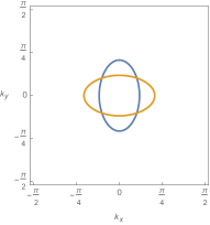
(a) $t_{\perp}=0$

(b) $t_{\perp}=0.005t_{a}$

Figure 2: The Fermi surface of the bilayer system in (a) the absence ($t_{\perp}=0$) and (b) the presence ($t_{\perp}=0.005t_{a}$) of an isotropic interlayer tunneling $t_{\perp}$. The parameters used are $t_{b}=t_{a}/3$ and $\mu=-2.5306t_{a}$. Note that we have zoomed in to an area that is one quarter of the full (unreconstructed) Brillouin zone.

We study a tight-binding model of electrons hopping on two coupled layers, each consisting of a square lattice with purely nearest-neighbor hopping elements. In the presence of an arbitrarily oriented magnetic field the Hamiltonian of this model has the form

$$H =\sum_{\langle\vec{r}_{i},\vec{r}_{j}\rangle;\sigma}\sum_{\lambda}-t_{\vec{r}_{i}-\vec{r}_{j};\lambda}\left(e^{i\Phi_{ij}}c^{{\dagger}}_{\vec{r}_{i},\lambda,\sigma}c_{\vec{r}_{j},\lambda,\sigma}+\mbox{H.c.}\right)$$

$$+\sum_{\vec{r}_{i};\sigma}\sum_{\lambda}4\pi\tilde{g}B\sigma c^{{\dagger}}_{\vec{r}_{i},\lambda,\sigma}c_{\vec{r}_{i},\lambda,\sigma}$$ (1)

$$-\sum_{\vec{r}_{i};\sigma}t_{\perp}\left(e^{i\Phi^{z}_{i}}c^{{\dagger}}_{\vec{r}_{i},1,\sigma}c_{\vec{r}_{i},2,\sigma}+\mbox{H.c.}\right)$$

where $c^{{\dagger}}_{\vec{r}_{i},\lambda,\sigma}$ is an electron creation operator at position $\vec{r}_{i}$ in layer $\lambda=1,2$ with spin $\sigma=\pm 1/2$, and $t_{\vec{r}_{i}-\vec{r}_{j};\lambda}$ denotes the appropriate hopping matrix element in layer $\lambda$, while $t_{\perp}$ is the (isotropic) hopping between each layer in the bilayer and $\tilde{g}$ controls the strength of Zeeman splitting. Here, $\Phi_{ij}=\int^{\vec{r}_{i}}_{\vec{r}_{j}}\bm{A}(\bm{r})d\bm{r}$ is the phase obtained by an electron hopping from site $\vec{r}_{j}$ to $\vec{r}_{i}$ in units in which $\hbar c/e=1$, while $\Phi^{z}_{i}$ is the phase obtained upon tunneling from one layer to the next at position $\vec{r}_{i}$. To obtain perpendicularly oriented elliptical pockets we set $t_{\hat{x};1}=t_{\hat{y};2}=t_{a}$, and $t_{\hat{y};1}=t_{\hat{x};2}=t_{b}$. In the absence of a magnetic field this Hamiltonian can be diagonalized to give the spectrum $E_{\pm}(\bm{k})$ where $\bm{k}=(k_{x},k_{y})$ is a two dimensional Bloch wavevector, with

$$E_{\pm}(\bm{k}) =\varepsilon_{+}(\bm{k})\pm\sqrt{\varepsilon^{2}_{-}(\bm{k})+t^{2}_{\perp}}$$ (2)

$$\varepsilon_{\pm}(\bm{k}) =-(t_{a}\pm t_{b})\cos(k_{x})-(t_{b}\pm t_{a})\cos{k_{y}}.$$ (3)

The Fermi surface with and without interlayer tunneling, with the choice of $t_{b}=t_{a}/3$ and a chemical potential of $\mu=-2.5306t_{a}$ is shown in Fig. 2.

In the absence of $t_{\perp}$, the addition of a magnetic field maps Eq.I to two copies of the Hofstadter problem. Upon coupling the layers, and for fields at arbitrary polar ($\theta$) and selected azimuthal angles ($\phi$), we can always pick a gauge that preserves translation symmetry along the in-plane direction of the magnetic field, $\hat{e}$. This allows us to take the Fourier transform along $\hat{e}$, and map Eq. I to a modified Harper’s equation. For simplicity, we will consider the case in which the magnetic field lies in the $y-z$ plane, with the generalization to arbitrary orientation deferred to Appendix A. With $\bm{B}=B\left(0,\sin{\theta},\cos{\theta}\right)$, we can choose the gauge

$$\bm{A}=\left(0,2\pi\Phi x,-2\pi\Phi x\tan{\theta}\right),$$ (4)

where $\Phi=B\cos\theta$ is the density of magnetic flux quanta per $x-y$ lattice plaquette (in units in which the plaquette area is $1$).

Upon Fourier transforming the Hamiltonian in the $\hat{y}$ direction we have $H=\sum_{k_{y},\sigma}\hat{H}_{k_{y},\sigma}$:

$$\hat{H}_{k_{y},\sigma}=\sum_{x,\lambda}\left\{t_{\hat{x},\lambda}\left(c^{{\dagger}}_{(x+1,k_{y});\lambda;\sigma}+c^{{\dagger}}_{(x-1,k_{y});\lambda;\sigma}\right)\right.$$

$$+\left.\left[2t_{\hat{y},\lambda}\cos{\left(2\pi\Phi x-k_{y}\right)}+\frac{4\pi\tilde{g}\Phi\sigma}{\cos\theta}\right]c^{{\dagger}}_{(x,k_{y});\lambda;\sigma}\right\}c_{(x,k_{y});\lambda;\sigma}$$

$$+\sum_{x}t_{\perp}\left(e^{-i2\pi\Phi a_{c}\tan{\theta}}c^{{\dagger}}_{x,k_{y};2;\sigma}c_{x,k_{y};1;\sigma}+\mbox{H.c.}\right)$$ (5)

where $a_{c}$ is the ratio of inter-bilayer spacing to the in-plane lattice constant. Eq. 5 has three properties that make it particularly amenable to numerical analysis: (i) the two spins $\sigma=\pm 1/2$ are decoupled and can be studied independently; 2) for arbitrary (irrational) values of $\Phi$, the spectrum of $H$ are independent of $k_{y}$ in the thermodynamic limitZhang et al. (2015), allowing us to suppress the $k_{y}$ summation; 3) the resulting one-dimensional problem concerning $\hat{H}_{k_{y},\sigma}$ is a block tri-diagonal matrix, whose inverse (and by extension, the Green’s function) can be calculated recursively as described in Appendix C, allowing efficient evaluations of its physical properties on system sizes as large as $L_{x}\sim 10^{7}$ sites along the $\hat{x}$ direction. In the remainder of the paper, we will be presenting calculations of QOs in the density of states (DOS) $\rho$ at chemical potential $\mu$, defined as

$$\rho(\mu) =-\frac{1}{\pi L_{x}}\text{Tr}\left(\text{Im}[\hat{G}]\right)$$ (6)

$$=-\frac{1}{\pi L_{x}}\sum_{x,\lambda}\text{Im}[G_{(x,\lambda),(x,\lambda)}(\mu)]$$

where $G_{(x,\lambda),(x,\lambda)}(\mu)$ represents the diagonal entry of the Green’s function

$$\hat{G}(\mu) =\left[\left(\mu+i\delta\right)\hat{I}-\hat{H}_{k_{y},\sigma}\right]^{-1},$$ (7)

The small imaginary term $i\delta$ gives a finite lifetime to the electrons and broadens the Landau levels.

Choice of Parameters

For a range of values, the qualitative aspects of our results do not depend sensitively on the values of most of the parameters that enter the model (with the exception of the pattern of magnetic breakdown, which we shall see is extremely sensitive to the value of $t_{\perp}$). However, to facilitate comparison with experiment, we chose parameters so that the $k$-space area enclosed by the elliptical Fermi pockets in the absence of interlayer tunneling is $S_{0}\approx 530T=1.91\%BZ$, the mean cyclotron effective mass $m^{*}\sim 1.6m_{e}$, and the electron’s spin $g$ factor is $g=2$. (See Appendix D for further discussion.) In the absence of any direct experimental information concerning the ellipticity of the Fermi pockets, we have arbitrarily adopted a moderate anisotropy, $\sqrt{3}$ (i.e. the major axis of the ellipse is $\sqrt{3}$ times larger than its minor axis.)

These considerations lead us to take $t_{b}=t_{a}/3$, $\mu=-2.5306t_{a}$, and $\tilde{g}=0.87$. Since all our calculations are carried out at $T=0$, the overall scale of energies is unimportant, but when referring to quantitative features of the electronic structure of YBCO, we will take $t_{a}=400$meV, in which case a characteristic inverse lifetime is $\delta=0.005t_{a}\approx(2\text{ ps})^{-1}$. We convert flux quanta per unit cell, $\Phi$, into units of the actual magnetic field $B$, by using a unit cell area of YBCO to be $\nu_{\text{unit cell}}=3.82\text{\AA}\times 3.89\text{\AA}$. This means that $B$ is related to the flux per unit cell (in units of the flux quantum) by $B=(h/e)\times(\Phi/\nu_{\text{unit cell}})\approx\Phi\times 27800$. The values of the interlayer tunneling, $t_{\perp}$, and the inverse lifetime $\delta$ are treated as unknowns; exploring the changes in the QO spectrum which occur as they vary is one of the principle purposes of this study.

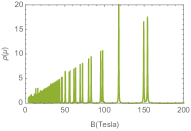
(a) $\rho$ vs.$B$

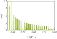
(b) $\rho$ vs. $1/B$

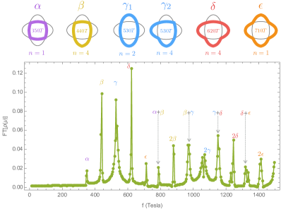
(c) Fourier transform of $(b)$

Figure 3: QOs of the DOS for very small broadening $\delta=0.0001t_{a}$ (long lifetimes) and $t_{\perp}=0.005t_{a}$, in the absence of a Zeeman coupling ($\tilde{g}=0$). Panels $(a)$ and $(b)$ show the calculated DOS $\rho$ vs. $B$ and $1/B$; panel $(c)$ is the Fourier transform of panel $(b)$. Each peak indicates a characteristic frequency of QOs and the corresponding semiclassical orbits are also illustrated above. The number of equivalent semiclassical orbits, $n$, is indicated below each orbit, and we have explicitly shown the two distinct classes of $\gamma$ orbits. A relatively large range of magnetic field is used $4T<B<1000T$ to capture all of the QO frequencies. The system size is $L_{x}=2^{23}$.

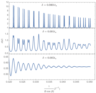
Figure 4: The evolution of QOs in the DOS $\rho(\mu)$ for various values of the inverse quasiparticle lifetime, $\delta$. The interlayer tunneling $t_{\perp}=0.005t_{a}$ and the rest of the parameters are detailed at the end of Sec. I.

II Semiclassical Considerations

Before undertaking the numerical solution of this model, it is useful to outline the results of a semiclassical analysis to anticipate the basic structure of the QOs in the simplest situation in which $B$ is perpendicular to the planes. As we are considering weakly coupled bilayers, we will always assume that $t_{\perp}\ll t\equiv\sqrt{t_{a}t_{b}}$, so the bilayer split Fermi surfaces have narrowly avoided crossings at four symmetry related points, as shown in Fig. 2b. Electrons adhere strictly to semiclassical orbits only so long as $\hbar\omega_{c}\ll t^{2}_{\perp}/t$ since magnetic breakdown at these four points becomes significant otherwise. (Here $\omega_{c}\sim\phi t$ is the cyclotron frequency.) Taking this magnetic breakdown into account, there are five distinct classes of semiclassical orbits, as shown in the middle panel of Fig. 3, each enclosing a $\bm{k}$-space area which, when converted into an oscillation frequency, correspond to five oscillation frequencies separated by $\Delta f\approx 90T$ for the model parameters we have defined. (These correspond to the frequencies labeled $\alpha$, $\beta$,$\gamma$, $\delta$, and $\epsilon$ in the spectrum in the lower panel of the figure, whose calculation is discussed in the next section).

The largest and smallest orbits represent the true structure of the Fermi surface, so these two frequencies ($\alpha$ and $\epsilon$) must dominate the QO spectrum when $\hbar\omega_{c}\ll t^{2}_{\perp}/t$. Conversely, in the limit $\hbar\omega_{c}\gg t^{2}_{\perp}/t$, where to good approximation we can set $t_{\perp}=0$, the spectrum is dominated by the central frequency ($\gamma_{1}$), in which the electron orbits are confined to a single plane of the bilayer, and hence correspond to the ellipses in Fig. 2a. More complex spectra, including those with the three peak structure seen in experiment, occur only when $\hbar\omega\sim t^{2}_{\perp}/t$. This, we shall see, allows us to estimate the magnitude of $t_{\perp}$ directly from experiment.

We will return again to a semiclassical analysis, below, in order to understand still more subtle features of the QO spectrum which appear when the magnetic field is tilted relative to the Cu-O plane.

III Numerical results

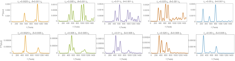
Figure 5: The raw Fourier transform the density of states oscillations as the interlayer tunneling $t_{\perp}$ is increased (left to right), and the inverse lifetime $\delta$ is increased (top to bottom). Larger values of $t_{\perp}$ suppress the central frequencies and enhance the satellite frequencies which correspond to orbits of the true bilayer split Fermi surface. Shorter quasiparticle lifetimes (larger $\delta$) lead to decreased harmonic content. The field range used here is $20T<B<100T$, with $2^{10}$ data points.

In presenting our results, we will adopt two complementary approaches. We first study an idealized theoretical limit of infinitesimally small broadening ($\delta\rightarrow 0$, i.e. infinite quasiparticle lifetime) and without Zeeman splitting, where a sharp Landau level structure of the density of states is present and easy to interpret. These numerical ‘experiments’ are done for a very large range of field strengths. We subsequently study the model over an experimentally realistic range of magnetic fields with the inclusion of Zeeman splitting, while tuning the broadening and interlayer tunneling $t_{\perp}$, and subsequently examining the angular dependences. While we predominantly highlight the robust qualitative features of this model, we also focus on the quantitative aspects of magnetic breakdown, which are treated exactly in our numerical studies.

In Fig. 3 we show the density of states as a function of magnetic field strengths for a $c$-directed field. The top panels show data where the broadening is infinitesimal at $\delta=0.0001t_{a}$ and there is no Zeeman splitting. Each Landau level is split due to the presence of two coupled layers, while the peaks in the density of states rise linearly with $B$ as expected for free fermions. The lower panel of Fig. 3 shows the Fourier transform of this data over a large range of magnetic fields ($4T<B<1000T$). Here the high harmonic content of the oscillations is clearly seen, with comparable-in-magnitude first and second harmonics. For the first harmonics, there are five peaks clustered around a central frequency of $f=530T$, as expected from semiclassical considerations, while at higher frequencies there are all the expected harmonic combinations giving rise to a complicated spectrum.

III.1 Dependence on interlayer tunneling and lifetime

We now study the model over an experimentally realistic range of magnetic fields with a finite Zeeman coupling, $\tilde{g}=0.87$. Fig. 4 and 5 show the evolution of the QOs as the interlayer tunneling $t_{\perp}$ and Landau level broadening $\delta$ are varied, where we have reduced the range of magnetic field to $20T<B<100T$ to conform roughly with the range explored by current experiments in YBCO. The figures are constructed from $2^{10}$ data points. As is clear from Fig. 4 the form of the oscillations is radically altered as the lifetime is decreased ($\delta$ in Eq. 7 is increased), with the sharp Landau level structure of the spectrum becoming broadened. This leads to oscillations with little harmonic content, while the amplitude of the oscillatory signal is also sharply suppressed.

Fig. 5 shows the Fourier transform of $\rho$ as both the interlayer tunneling $t_{\perp}$ is increased (from left to right) and the inverse lifetime $\delta$ is increased (from top to bottom). Several qualitative features of the results are immediately apparent. (1) As the inverse lifetime $\delta$ is increased (and the oscillations of $\rho$ become less singular), the peaks in the Fourier transform are also broadened while the higher frequency peaks are preferentially suppressed in amplitude, leading to oscillations with little harmonic content. This has a simple semiclassical interpretation: higher frequency peaks correspond to longer semiclassical orbits and so are suppressed in amplitude by the decreasing quasiparticle lifetime.Bergemann et al. (2003) (2) The competition between different semiclassical orbits is sensitively controlled by the interlayer tunneling $t_{\perp}$: as $t_{\perp}$ is increased, the gaps between bonding and anti-bonding Fermi surfaces increase, and the weight of QOs rapidly shifts from the central frequency at $530T$ (corresponding to the 3rd orbit in Fig.  3 which involves two magnetic breakdowns across the true Fermi surface of the bilayer) to the side frequencies at $(530\pm 90)T$ (corresponding to the second and fourth semiclassical orbits in Fig.  3), and is eventually dominated by the outermost frequencies at $(530\pm 180)T$ (reflecting the ‘true’ bonding and anti-bonding Fermi surfaces of the bilayer).

Indeed, a particularly appealing feature of our approach is its exact treatment of magnetic breakdown. The immediate quantitative observation from Fig. 5 is that maintaining the large (experimentally observed) ratio of the amplitude of the central $530T$ frequency to that of the satellite frequencies at $530\pm 90T$ requires very small values of the interlayer tunneling $t_{\perp}<0.01t_{a}$. This is at least an order of magnitude below the typical values of $t_{\perp}\sim 0.1t_{a}$ assigned by band structure studiesAndersen et al. (1995); Elfimov et al. (2008) and ARPES studiesFournier et al. (2010) on overdoped YBCO, but agrees remarkably with ARPES measurements of the underdoped regime. We discuss the consequences of this observation in Sec. IV.

III.2 Polar angle ($\theta$) dependence of the QOs

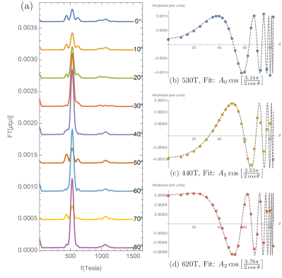
Figure 6: (a) The Fourier transform of the DOS QOs for various polar angles $\theta$ of the magnetic field $\vec{B}$ (different angles have been arbitrarily offset). (b)-(d) Extracted peak heights in the Fourier transform (we have used both amplitude and phase information) versus the polar angle $\theta$. The parameters are $\delta=0.005t_{a}$, $t_{\perp}=0.005t_{a}$. The dashed lines are the theoretical fits of the angular dependence due to spin splitting (Eq. 8) which is caused by Zeeman effect.

We now move on to cases where the magnetic field is tilted away from the principal $c$-axis of this model and study the dependence of the QOs on the polar and azimuthal angles, $\theta$ and $\phi$; we also comment briefly on the corresponding dependence seen in YBCO. Key experimental features include the presence of spin zeroes near $\theta\approx 51.5^{\circ}$ and $\theta\approx 63.5^{\circ}$, with the notable absence of a Yamaji angle that is typical of simple $s$-wave warping of a three dimensional Fermi surface. Spin zeros (as well as the general $\theta$ dependence) arise due to Zeeman splitting of spinful electrons. This coupling effectively shifts the chemical potential (and hence the area of each orbit) oppositely for each species $\sigma$, by an amount that is proportional to the applied field $\delta f=\sigma\gamma B$. Such a $B$ dependent shift of the Fermi surface area for each spin species becomes a shift of the bare (spinless) frequency $f_{0}$ of oscillations, so that the amplitude of oscillations for the $p$’th harmonic acquires a field independent (but $\theta$ dependent) amplitude:

$$\rho\left(\frac{1}{B},\theta\right) \propto\sum_{\sigma=\pm 1/2}\cos{\left(2\pi p\frac{(f_{0}+\sigma\gamma B)}{B\cos{\theta}}\right)}$$ (8)

$$=2\cos{\left(\frac{\pi p\gamma}{\cos{\theta}}\right)}\cos{\left(2\pi p\frac{f_{0}}{B}\right)}.$$

A more careful analysis shows that this field independent amplitude takes the form $A(\theta)=\cos{\left(\pi pg\frac{m^{*}}{2m_{e}\cos{\theta}}\right)}$ where in practice the factor $\pi pgm^{*}/2m_{e}$ is related to our definition of $\tilde{g}$ as discussed in Appendix D.

Fig. 6(a) shows the polar angle $\theta$ dependence of the Fourier transform of QOs for the model system in Eq. I. The azimuthal angle is fixed at $\phi=45^{\circ}$ throughout the calculation. As expected, no Yamaji-like resonance is seen because of the absence of a truly three-dimensional dispersion. Fig. 6(b)-(d) shows the $\theta$ dependence of the QO amplitude $A(\theta)$ at the three main frequencies. We see characteristic spin-zeroes in the primary frequency $f=530T$ near $\theta_{0}=51.5^{\circ}$ and $\theta_{1}=63.5^{\circ}$. The dashed lines show fits of the amplitude to the form given in Eq. 8 - remarkable agreement is found. We note that the positions of the spin zeroes are different for the QOs at frequencies $440T$, $530T$ and $620T$, despite the fact that the $g$-factor (our parameter $\tilde{g}$) has been defined to be the same for all orbits. This robust feature of our model can be attributed to the different effective mass of the these three orbits which enters the form $\cos{\left(\pi pgm^{*}/{2m_{e}\cos{\theta}}\right)}$, and is explored further in Appendix D.

III.3 Azimuthal angle ($\phi$) dependence of the QOs

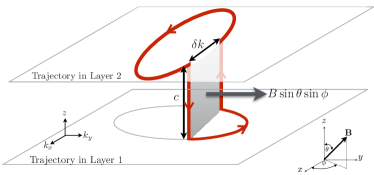
(a) 3D Cartoon plot of semiclassical orbit in the bilayer

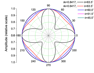
(b) Corresponding $\phi$ dependence of the QOs at $620T$ and $440T$ given in Eq. 9

Figure 7: (a) A schematic diagram showing how the in-plane component of the flux enclosed by a given semiclassical orbit ($\delta$ orbit in Fig. 3) is determined. The red curve is the semiclassical orbit, while grey ellipses are the Fermi surfaces. Note that the in-plane directions are in momentum space, while the vertical separation is in real space. The vertical region enclosed (shaded gray) has a (real space) area of $\delta k\ell^{2}_{B}c$. (b) The $\phi$ dependence of QO amplitude $A_{1}(\phi)$ as in Eq. 9 for various values of the polar angle $\theta$ for $\delta k=0.6417$ defined in our model as well as the case of a larger $\delta k=0.8417$. The anisotropy is clearly more apparent for larger $\theta$ and/or $\delta k$.

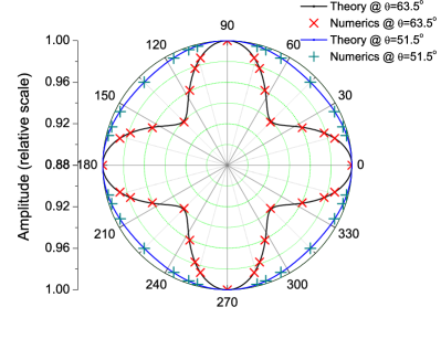
Figure 8: The relative amplitude of the QOs at frequency $620T$ for polar angles $\theta=63.5^{\circ}$ and $\theta=51.5^{\circ}$, respectively. The QO amplitude at $\phi=0$ is maximal and set as the unit $1$ for each of the data sets. The solid curve is the theoretical expectation value according to Eq. 9 and the expected $C_{4}$ rotation symmetry is clearly present. The parameters used in our numerical calculations of the DOS QOs are $t_{\perp}=0.005$, $\delta=0.001$ and $11T<B<100T$.

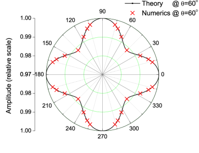
Figure 9: The relative amplitude of the QOs at frequency $530T$ for polar angles $\theta=60^{\circ}$. The solid curve is the fit to theoretical form given by Eq. 10 with $M=-13.5$. The parameters used in our numerical calculations of the DOS QOs are $t_{\perp}=0.005$, $\delta=0.001$ and $11T<B<100T$.

Another notable feature of QO experiments in YBCO is the dependence of the amplitude of the oscillations on the azimuthal angle $\phi$. The oscillation amplitudes exhibit a four-fold anisotropy, which increases with increasing polar angle $\theta$. Here, we show that these features can be reproduced in our model of a single bilayer, with the caveat that strong anisotropy is only natural for selected orbits that involve both layers of the bilayer ($\beta$ orbit at $440T$, $\delta$ orbit at $620T$ and $\gamma_{2}$ orbit at $530T$).

In analyzing the behavior of QOs for different azimuthal angles, much information can be gleaned from semiclassical intuitions. First, note that the semiclassical orbits $\gamma_{1}$ at the central $530T$ frequency in Fig. 3 are predominantly confined to a single layer of the bilayer. Such $2d$ orbits are only affected by the field perpendicular to the layer, therefore no observable azimuthal dependence is expected. On the other hand, all other semiclassical orbits shown in Fig. 3 involve tunneling events from one layer to the next, upon which electrons may obtain a phase proportional to the horizontal magnetic field $B\sin{\theta}$. This means that there is weak four-fold dependence arising from $\gamma_{2}$ orbits, wherever the signal is dominated by the $530T$ frequency; conversely, a large four-fold modulation arises from the $530\pm 90T$ frequencies, and so is pronounced near to spin zero angles $\{\theta_{0},\theta_{1}\}$ of the main $530T$ frequency.

Within the semiclassical framework, we can obtain an analytic expression for the amplitude as a function of azimuthal angle $\phi$ by determining the amount of in-plane directed magnetic flux enclosed by a given breakdown orbit. Fig 7(a) shows the geometry of a particular breakdown orbit for QOs at $620T$, where the total horizontal flux is the real space area corresponding to the shaded region, multiplied by the field component $B\sin{\theta}\sin{\phi}$. Semiclassically, we find the real space area enclosed by the orbit to be $\delta k\ell^{2}_{B}\times c$, where $\ell^{2}_{B}=h/eB\cos{\theta}$ is the square of the magnetic length, and $\delta k$ is the distance between the (avoided) crossings of the Fermi surfaces (see Fig. 7(a)). Thus, the in-plane flux enclosed by this orbit is $\Phi_{yz}=\delta k\frac{\hbar}{eB}c\times B\tan\theta\cos\phi=c\delta k\tan\theta\sin\phi$ with our choices of units. Similarly, there are three other possible enclosed fluxes related by $C_{4}$ rotations, and given by $\Phi_{-yz}=-\Phi_{yz}$, and $\Phi_{\pm xz}=\pm c\delta k\tan\theta\cos\phi$. The resulting $\Phi_{j}$, $j=\pm xz,\pm yz$ each give an additional constant initial phase to the in-plane fluxes that determine the QOs of the corresponding reconstruction, which add up to give the overall amplitude:

$$A_{1}(\phi) \propto\sum_{j}\exp{\left(i\Phi_{j}\right)}\propto 2\cos\Phi_{xz}+2\cos\Phi_{yz}$$ (9)

$$\propto 2\cos\left(c\delta k\tan\theta\cos\phi\right)+2\cos\left(c\delta k\tan\theta\sin\phi\right)$$

Examples of the azimuthal angular dependence given by Eq. 9 are shown in Fig. 7(b), whose form guarantees $C_{4}$ rotation symmetry. For smaller values of the polar angle $\theta$ (and thus a smaller overall factor $c\delta k\tan\theta$), the $\phi$ angular dependence is suppressed. We note that the magnitude of the anisotropy depends sensitively on $\delta k$. An example of the QO amplitude variation for a larger $\delta k=0.8417$ as compared to the original $\delta k=0.6417$ is also included in Fig. 7(b).

It is straightforward to verify that the angular dependence of the QOs at $440T$ has the same result as Eq. 9, while at $530T$ we need to consider both the $\gamma_{1}$ and $\gamma_{2}$ orbits:

$$A^{\prime}_{1}(\phi) \propto M+2\cos\left(c\delta k\tan\theta(\cos\phi+\sin\phi)\right)$$

$$+2\cos\left(c\delta k\tan\theta(\cos\phi-\sin\phi)\right)$$ (10)

where $M$ is a complex constant for the contribution from $\gamma_{1}$ orbits and sensitively depends on the parameters including $t_{\perp}$ and $B$.

Another immediate consequence of this expression is that the maximum in QO amplitudes at the side frequencies at $(530\pm 90)T$ occurs when the field is aligned with the principal axes of the ellipses. Given that experimentally, the maximum of the oscillation amplitudes is seen to occur for fields along the $a$ and $b$ crystallographic directions, it is natural that the principal axes of such elliptical pockets must lie along the $a$ and $b$ directions, i.e. such azimuthal dependence seemingly rules out proposals where the principal axes of the Fermi pockets are oriented at $45^{\circ}$ to the $a$ and $b$ crystallographic directions.

Returning to the model at hand, we calculated numerically the density of states QOs with selected values of the azimuthal angle $\tan\phi=0,1,2,3,4$ (plus symmetry related values) and various polar angles. The resulting QO amplitudes at frequency $620T$ and polar angles $\theta=63.5^{\circ}$ and $\theta=51.5^{\circ}$ are shown in Fig. 8 and is fully consistent with the semiclassical expression derived in Eq. 9. In particular, the selected $\theta$ values are the spin zeros of the central frequency at $f=530T$ of the QOs, where the effect of the side frequencies at $(530\pm 90)T$ are enhanced. In addition, four-fold anisotropy is also seen for the QO amplitudes at frequency $530T$ and polar angle $\theta=60^{\circ}$ as shown in Fig. 9, and fits well to Eq. 10 with parameter $M=-13.5$.

IV Implications for the cuprates

We have shown that a simple model of criss-crossed elliptical electron pockets can reasonably account for the most striking experimental observations of QOs in the bilayer cuprate YBCO. In particular, we have shown that a three peak structure in the Fourier transform of QOs follows naturally from the ansatz of broken mirror symmetry and weak bilayer splitting. The choices of tight-binding and Zeeman-splitting parameters that best capture this physics have been analyzed semi-quantitatively. We have also demonstrated that major features of both the azimuthal and polar angular dependence of the QOs can be qualitatively reproduced by this simplified model of a single bilayer.

A central feature of our analysis involves the small effective interlayer tunneling $t_{\perp}$ required to account for the prominence of the central $530T$ frequency relative to those at $530\pm 90T$. In certain situations, a singular $k$ dependenceAndersen et al. (1995); Chakravarty et al. (1993); Elfimov et al. (2008) of the bare interlayer tunneling, $t_{\perp}^{(0)}(k)\approx t_{\perp}^{(0)}(\cos{k_{x}}-\cos{k_{y}})^{2}$, arises due to the local quantum chemistry. In this case the small value of the effective $t_{\perp}$ could reflect the location of the electron pockets along the “nodal” direction in the Brillouin zone where $|k_{x}|=|k_{y}|$, rather than any non-trivial many-body effect. However, there are strong reasons to doubt that the bilayer tunneling in YBCO has such strong $k$ dependence. On theoretical grounds, LDA studiesAndersen et al. (1995); Elfimov et al. (2008) have found that the tunneling between the ‘dimpled’ planes of a YBCO bilayer remains substantial even along the nodal direction with $t^{(0)}_{\perp}(\bm{k}_{n})\approx 120$meV, compared to an antinodal value of $t^{(0)}_{\perp}(\bm{k}_{an})\approx 150$meV.

This LDA prediction is supported by ARPES measurements on YBCO in the overdoped regimeFournier et al. (2010) where an almost isotropic bilayer splitting of $\Delta\varepsilon_{\bm{k}_{n}}=2t_{\perp}(\bm{k}_{n})=2Zt^{(0)}_{\perp}(\bm{k}_{n})\approx 130$meV in the nodal direction, compared to an antinodal splitting $\Delta\varepsilon_{\bm{k}_{an}}\approx 150$meV leads to a near isotropic quasiparticle weight of $Z\approx 0.5$. This is in sharp contrast to underdoped samples, where despite the theoretical (LDA) prediction of a doping independent $t^{(0)}_{\perp}$, the nodal bilayer splitting is difficult to resolve. These experiments give an upper bound of the nodal quasiparticle weight in the underdoped regime of $Z_{n}<0.065$, while an estimate based on the rescaled values of the spectral weight yields $Z_{n}\approx 0.03$. Such estimates agree remarkably well with our estimate of the effective value of $t_{\perp}$ necessary to account for the QO’s in underdoped YBCO. The constraint of the quasiparticle weight $\tilde{Z}\lesssim 0.05$, strongly suggests that the effective Fermi liquid parameter $t_{\perp}=\tilde{Z}t^{(0)}_{\perp}$ is renormalized significantly downwards.

IV.1 Comparison with previous proposals

There have been many proposalsChakravarty et al. (2001); Millis and Norman (2007); Harrison and Sebastian (2011); Eun et al. (2012); Harrison and Sebastian (2012); Lee (2014); Allais et al. (2014); Wang and Chubukov (2014); Maharaj et al. (2014); Russo and Chakravarty (2015); Harrison et al. (2015); Briffa et al. (2015) for the origin of the Fermi surface reconstruction in the cuprates. Given recent observations of (seemingly ubiquitousTranquada et al. (1994, 1995); Fujita et al. (2004); Howald et al. (2003); Hoffman et al. (2002); Hanaguri et al. (2004); Fink et al. (2009); Laliberté et al. (2011); Chang et al. (2012); Ghiringhelli et al. (2012); Achkar et al. (2012); Doiron-Leyraud et al. (2013); LeBoeuf et al. (2013); He et al. (2014); Tabis et al. (2014); Forgan et al. (2015)) incommensurate CDW order, a prime candidate for the Fermi surface is one where nodally located electrons pockets are produced by incommensurate CDWs which are at least bi-axial, involving ordering at $\vec{Q}_{x}=(Q,0,1/2)$ and $\vec{Q}_{y}=(0,Q,1/2)$. This idea, along with the invocation of breakdown orbits due to bilayer splitting to account for the three peak structure of the Fourier transform, was first advanced by Harrison, Sebastian and co-workersHarrison and Sebastian (2011); Sebastian et al. (2012a). In this scenario, a diamond shaped, nodally located electron pocket is split by bilayer tunneling (with the above mentioned $(\cos{k_{x}}-\cos{k_{y}})^{2}$ form factor), with all three observed frequencies involving orbits where the electron tunnels from one layer to the next. The nodal location also serves to suppress simple isotropic ($s$-wave) hoping in the $c$ axis direction, leading to an absence of a Yamaji resonance.

The model discussed in the present paper, while similar in spirit to that of Harrison and Sebastian, possesses crucial differences of symmetry and effective dimensionality. Under the assumption that QO experiments probe the physics of a single bilayer, mirror symmetry between the two layers of this bilayer must be broken in order for breakdown orbits to be present in a purely $c$-axis directed magnetic field – otherwise a conserved bilayer parity associated with the split Fermi surfaces would prevent all magnetic breakdown (see Appendix B). Indeed, there is evidence for such broken symmetry in the low field charge order.Forgan et al. (2015); Briffa et al. (2015) Once mirror symmetry is broken, a natural consequence is that the central $532T$ frequency reflects a semiclassical orbit where electrons are confined to a single layer of the bilayer, and if so, is naturally the most prominent in the regime of small interlayer tunneling. We have demonstrated that the experimental observations can be generally accounted for in the context of a minimal model of a single bilayer. In contrast to previous proposals, this model requires no specific $3d$-structure of the Fermi surface, and makes no specific assumptions about the nature of the order that reconstructs the Fermi surface; given that recent high field X-ray scattering experimentsGerber et al. (2015) have given evidence of an unexpected, distinct high-field character of the CDW order, we view this lack of specificity as a virtue.

IV.2 Further tests from experiments in YBa₂Cu₃O_6.58

The magnetic breakdown scenario makes two specific predictions for QO experiments in bilayer cuprates:

1. Oscillations taken over a sufficiently large field range should show five spectral features distributed symmetrically about the main frequency, plus multiple higher harmonics from combination orbits.

2. The weight of the various frequency components of the quantum oscillations should be field-dependent, with orbits that require fewer breakdown events dominating at low fields.

Fig. 10 shows torque magnetometry data taken on YBa₂Cu₃O_6.58 at 1.5 kelvin. Multiple spectral components, beyond the three main peaks identified in previous studies but consistent with those presented in section III, are clearly visible with this extended field range (18.5 to 62.6 Tesla). Appendix E demonstrates that these peaks (particularly $\alpha$ and $\epsilon$) are not artifacts of the Fourier transform, but are instead physical components of the oscillatory signal.

Transforming the data over a limited low-field range, from 18.5 to 26 T (blue curve in Fig. 10), shows that the main 530 T peak is indeed no longer dominant. Semiclassically Shoenberg (1984), the probability of tunneling through any one of the four junctions between the bilayer split Fermi surfaces (Fig. 2) is $P=e^{-B_{0}/B}$, where $B_{0}$ is the characteristic breakdown field. The probability of avoiding breakdown (Bragg reflection) at a junction is $(1-P)$. While this expression is not exact (unlike the breakdown treatment in section III), particularly at fields large compared to $B_{0}$, it gives intuition as to why the spectral weight shifts at lower fields: the $\gamma$ orbit shown in Fig. 3 requires four breakdown events, while the $\alpha$ ($\epsilon$) orbit requires none and the $\beta$ ($\delta$) orbit requires two. Note that the field range used to obtain the blue curve in Fig. 10 is insufficient to resolve the splitting of these peaks. Finally, the dominance in amplitude of lower frequencies over higher frequencies originatesBergemann et al. (2003) in the suppression of larger orbits due to quasiparticle scattering.

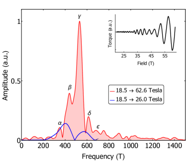
Figure 10: Fourier transform of torque quantum oscillation in YBa₂Cu₃O_6.58. Analysis of the full field range, from 18.5 to 62.6 Tesla (red curve), reveals spectral features not present in Fig. 1, but that correspond well with the frequencies shown in Fig. 3. Analysis of the oscillations between 18.5 and 26 Tesla only (blue curve) show that spectral weight is shifted away from the main $\gamma$ peak, and toward the sidelobes. The blue curve has been multiplied by a factor of 10 and truncated at 700 T for clarity. Note that spectral features below $\approx 150$ T are removed as part of the background-subtraction procedure, and thus this data does not address the possibility of a 90 T frequency that has been reported in transport measurements Doiron-Leyraud et al. (2015).

V Acknowledgements

We acknowledge extremely useful discussions with A. Damascelli, N. Harrison, G. Lonzarich, A. P. Mackenzie, C. Proust, S. Sebastian, L. Taillefer and J. Tranquada. This work was supported in part by the US Department of Energy, Office of Basic Energy Sciences under contract DE-AC02-76SF00515 (A.V.M.), Stanford Institute for Theoretical Physics (Y.Z.), the US Department of Energy Office of Basic Energy Sciences “Science at 100 T,” (B.J.R.) and the National Science Foundation through Grant No. DMR 1265593 (S.A.K.). The National High Magnetic Field Laboratory facility is funded by the Department of Energy, the State of Florida, and the NSF under cooperative agreement DMR-1157490 (B.J.R).

Appendix A Form of the Hamiltonian for general angles $\phi$

For additional azimuthal angles as $\tan\phi=1/M$ where $M\in\mathbb{Z}$ (or equivalently $\tan\phi=M$ by symmetry):

$$\vec{B}=B\left(\hat{z}\cos\theta+\hat{x}\sin\theta M/\sqrt{M^{2}+1}+\hat{y}\sin\theta/\sqrt{M^{2}+1}\right)$$ (11)

we can no longer keep the translation symmetry along the $\hat{y}$ direction for arbitrary $B$ with the chosen Landau gauge, however, we can define the new magnetic unit cell with the new lattice vectors $\hat{x}^{\prime}=\hat{x},$ and $\hat{y}^{\prime}=M\hat{x}+\hat{y}$ along $\vec{B}$ in plane or equivalently $x^{\prime}=x-My$, $y^{\prime}=y$. Once again we can choose a proper gauge so that the translation symmetry along the $\hat{y}^{\prime}$ direction is preserved:

$$\bm{A} =\left(0,2\pi\Phi(x-My),-2\pi\Phi a_{c}\tan\theta(x-My)/\sqrt{M^{2}+1}\tan{\theta}\right)$$

$$=\left(0,2\pi\Phi x^{\prime},-2\pi\Phi x^{\prime}a_{c}\tan\theta/\sqrt{M^{2}+1}\right)$$ (12)

where $\Phi=B\cos\theta$ is the magnetic flux through the plaquette in the $x-y$ plaquette, and $\Phi a_{c}\tan\theta/\sqrt{M^{2}+1}$ is the flux through the $x-z$ plaquette. The hopping matrix elements no longer depend on $y^{\prime}$, therefore we can Fourier transform into the corresponding $k_{y}^{\prime}$ momentum basis. The resulting Hamiltonian (for each $k_{y}^{\prime}$ and spin $\sigma$) becomes:

$$\hat{H}_{k_{y}^{\prime},\sigma} = \underset{x,\lambda}{\sum}t_{x,\lambda}\left[c_{x+1,\lambda}^{\dagger}c_{x,\lambda}+\mbox{H.c.}\right]+\frac{4\pi\tilde{g}\Phi\sigma}{\cos\theta}c_{x,\lambda}^{\dagger}c_{x,\lambda}$$

$$+ \underset{x,\lambda}{\sum}t_{y,\lambda}\left[c_{x-M,\lambda}^{\dagger}c_{x,\lambda}\exp\left(i2\pi\Phi x-k_{y}^{\prime}\right)+\mbox{H.c.}\right]$$

$$+ \underset{x}{\sum}t_{\perp}\left[c_{x,2}^{\dagger}c_{x,1}\exp\left(i2\pi\Phi xa_{c}\tan\theta/\sqrt{M^{2}+1}\right)+\mbox{H.c.}\right]$$

where we have suppressed the $k_{y}^{\prime}$ and $\sigma$ labels in the fermion operators. The Hamiltonian is still block tri-diagonal and its physical properties including DOS can be efficiently calculated using recursive Green’s function method.

Appendix B Mirror symmetry and the absence of breakdown frequencies

(a) Mirror symmetric

(b) Broken mirror symmetry

Figure 11: Fourier transforms of QOs in the density of states for two models (a) with mirror symmetry and (b) without mirror symmetry. In (a) we consider identical Fermi surfaces with an interlayer tunneling of the form $t_{\perp}(\bm{k})=t_{\perp}\cos^{2}(2k_{y})$, while in (b) the mirror symmetry is weakly broken by considering orthogonal Fermi surfaces with a weak mass anisotropy ($t_{b}=0.95t_{a}$) and the interlayer tunneling is once more $t_{\perp}(\bm{k})=t_{\perp}\cos^{2}(2k_{y})$. The bilayer bonding and anti bonding Fermi surfaces are almost identical in both cases, yet the QO frequencies are dramatically different: mirror symmetry forbids breakdown orbits in (a).

Here we discuss in further detail the absence of magnetic breakdown when a mirror symmetry relating the two planes of the bilayer is present. The essence of this symmetry argument is the following: in the presence of a magnetic field semiclassical dynamics correctly captures the motion of electrons, while magnetic breakdown is allowed as long as there exist matrix elements that take electrons from one orbit to the next. However, if there is a mirror plane perpendicular to the magnetic field, the mirror parity of the states remains a good quantum number even in the presence of a magnetic field. There are necessarily no matrix elements between states with different quantum numbers, and so breakdown processes are forbidden by this symmetry. We emphasize that this argument is also applicable in the limit of a single bilayer, i.e. when $k_{z}$ is not a good quantum number.

This symmetry may be viewed at a more operational level by considering the Hamiltonian of a bilayer with identical dispersions $\varepsilon(\bm{k})$ in each layer. In the absence of a field, this takes the form

$$H =\sum_{\bm{\bm{k}}}\Psi_{\bm{k}}\hat{H}_{\bm{\bm{k}}}\Psi_{\bm{k}}=\sum_{\bm{k}=k_{x},k_{y}}\begin{matrix}(c^{{\dagger}}_{\bm{k},1}&c^{{\dagger}}_{\bm{k},2})\\ &\\ \end{matrix}\begin{pmatrix}\varepsilon(\bm{k})&t_{\perp}(\bm{k})\\ t_{\perp}(\bm{k})&\varepsilon(\bm{k})\end{pmatrix}\begin{pmatrix}c_{\bm{k},1}\\ c_{\bm{k},2}\end{pmatrix}$$ (14)

where $t_{\perp}(\bm{k})$ is the (in general) momentum dependent tunneling between layers.

Mirror symmetry relating the two layers of the bilayer is akin to the statement that the Hamiltonian commutes with the $x$-Pauli matrix, $\hat{\tau}_{x}$:

$$\left[\hat{H}_{\bm{k}},\hat{\tau}_{x}\right]=0,\,\,\qquad\text{where}\,\,\,\hat{\tau}_{x}=\begin{pmatrix}0&1\\ 1&0\end{pmatrix}$$ (15)

It should be clear that this operation swaps the two planes of the bilayer, and so implements that mirror operation that we are referring to. The addition of a magnetic field $\bm{B}$ is typically implemented via a Peierls substitution, resulting in a dramatic change to the structure of the Hamiltonian and eigenstates. In particular, working in Landau gauge we only preserve translation invariance in a single direction, so in general the eigenstates will be labeled by a generalized Landau level index, $n$, and transverse momentum, $k_{y}$. However, as long as the magnetic field does not break this mirror symmetry, i.e. $\bm{B}=B_{z}\hat{z}$, it remains the case that eigenstates of $\hat{H}$ are also eigenstates of $\hat{\tau}_{x}$, i.e.

$$[\hat{H},\hat{\tau}_{x}] =0$$ (16)

$$\hat{H}\lvert n,k_{y},\pm\rangle =E_{(n,k_{y},\pm)}\lvert n,k_{y},\pm\rangle$$ (17)

$$\hat{\tau}_{x}\lvert n,k_{y},\pm\rangle =\pm\lvert n,k_{y},\pm\rangle$$ (18)

Note that these are the exact eigenstates of the system, and they are necessarily orthogonal. Also notice that none of these statements depend on the form of the interlayer tunneling $t_{\perp}(\bm{k})$.

The absence of magnetic breakdown is then most easily understood by considering the structure of the energy spectrum. Oscillations in any physical quantity arise because of periodicity in the structure of the energy spectrum as a function of $1/B$. The discrete two-fold mirror symmetry means that the Hamiltonian separates into two independent blocks, so that the energy spectrum for these $+$ and $-$ sectors can be solved independently. Because these sectors can be treated as independent systems, as the magnetic field is varied, each sector produces a single fundamental frequency in quantum oscillations. This results in two (possibly degenerate) quantum oscillation frequencies, with neither magnetic breakdowns nor beat (sum or difference) frequencies.

Fig.  11(a) and 11(b) provide confirmation of these symmetry arguments. In Fig. 11(a) we have considered identical dispersions $\varepsilon(\bm{k})=-2t(\cos{k_{x}}+\cos{k_{y}})-\mu$ with $t=1$ and $\mu=-2.8t$, and $t_{\perp}(\bm{k})=-0.1t\cos^{2}{(2k_{y})}$. This form of the interlayer tunneling is both technically simple to implement, and produces nodes in the bilayer splitting. As is clear from the Fourier transform, no magnetic breakdown is present, and only two fundamental frequencies are seen when the interlayer tunneling is present. In Fig. 11(b) we weakly break the symmetry by considering dispersions of the form $\varepsilon(\bm{k})=-2(t_{a}\cos{k_{x}}+t_{b}\cos{k_{y}})-\mu$ in one layer, and $\varepsilon(\bm{k})=-2(t_{b}\cos{k_{x}}+t_{a}\cos{k_{y}})-\mu$ in the next layer, with $t_{b}=0.95t_{a}$. In the absence of interlayer tunneling, only one frequency is seen in QOs (these pockets have identical areas), but a finite interlayer tunneling leads to multiple breakdown orbits.

Appendix C Recursive Green’s function method for the DOS of a tri-diagonal block Hamiltonian

As is shown in the main text, the Hamiltonian in $k_{y}$ and $\sigma$ basis only involves finite-range coupling and is block tri-diagonal

$$\hat{H}_{k_{y},\sigma} =\begin{pmatrix}\ddots&\vdots&&&\\ \ldots&\hat{h}_{x-1,\sigma}&\hat{t}&&\\ &\hat{t}&\hat{h}_{x,\sigma}&\hat{t}&\\ &&\hat{t}&\hat{h}_{x+1,\sigma}&\ldots\\ &&&\vdots&\ddots\end{pmatrix},$$ (19)

$$\quad\hat{h}_{x,\sigma} =\begin{pmatrix}2t_{y,1}\cos(2\pi\Phi x-k_{y})+\frac{4\pi\tilde{g}B\sigma}{\cos\theta}&t_{\perp}\exp(i2\pi\Phi a_{c}x\tan{\theta})\\ t_{\perp}\exp(-i2\pi\Phi a_{c}x\tan{\theta})&2t_{y,2}\cos(2\pi\Phi x-k_{y})+\frac{4\pi\tilde{g}B\sigma}{\cos\theta}\end{pmatrix},$$ (20)

$$\quad\hat{t} =\begin{pmatrix}t_{x,1}&0\\ 0&t_{x,2}\end{pmatrix}$$ (21)

We are interested in the DOS $\rho_{\sigma}(\mu)$ of spin $\sigma$ electrons at chemical potential $\mu$ defined as

$$\rho_{\sigma}(\mu)=-\frac{1}{\pi L_{x}}\text{Tr}\left(\text{Im}[\hat{G}_{\sigma}(\mu)]\right)$$ (22)

$$\hat{G}_{\sigma}(\mu)=\left[(\mu+i\delta)\mathbb{I}-\hat{H}_{k_{y},\sigma}\right]^{-1}$$ (23)

where we have used the fact that the physical quantities are independent of $k_{y}$ in the thermodynamic limit to suppress the summation over the $k_{y}$ index.

To obtain the diagonal elements of the Green’s function $\hat{G}_{\sigma}(\mu)$, we note the inverse of the following block tri-diagonal matrix may be calculated recursively

$$\hat{G}^{-1}_{\sigma}(\mu)=(\mu+i\delta)\mathbb{I}-\hat{H}_{k_{y},\sigma}=\begin{pmatrix}\bm{a}_{1,1}&\bm{a}_{1,2}&&&\\ \bm{a}_{2,1}&\bm{a}_{2,2}&\bm{a}_{2,3}&&\\ &\bm{a}_{3,2}&\bm{a}_{3,3}&\bm{a}_{3,4}&\\ &&\ddots&\ddots&\ddots\\ \end{pmatrix}$$ (24)

where $\bm{a}_{i,i}=(\mu+i\delta)\mathbb{I}-\hat{h}_{x,\sigma}$ and $\bm{a}_{i,i+1}=\bm{a}_{i,i+1}=\hat{t}$. This is accomplished by the following recursive algorithm, which consists of two independent sweeps (and hence the computation is linear in the size $L_{x}$):

For increasing $i=1,2,\ldots,N-1$ we define

$$\bm{c}^{L}_{i}=-\bm{a}_{i+1,i}(\bm{d}^{L}_{i})^{-1},$$ (25)

with $\bm{d}^{L}_{1}=\bm{a}_{1,1}$ and $\bm{d}^{L}_{i}=\bm{a}_{i,i}+\bm{c}^{L}_{i-1}\bm{a}_{i-1,i}$; for decreasing $i=N,N-1,\ldots,2$ we define

$$\bm{c}^{R}_{i}=-\bm{a}_{i-1,i}(\bm{d}^{R}_{i})^{-1},$$ (26)

where $\bm{d}^{R}_{N}=\bm{a}_{N,N}$ and $\bm{d}^{R}_{i}=\bm{a}_{i,i}+\bm{c}^{R}_{i+1}\bm{a}_{i+1,i}$, then the diagonal blocks of $\hat{G}_{\sigma}(\mu)=\left[(\mu+i\delta)\mathbb{I}-\hat{H}_{k_{y},\sigma}\right]^{-1}$ are given by

$$\hat{G}_{i,i}=(-\bm{a}_{i,i}+\bm{d}^{L}_{i}+\bm{d}^{R}_{i})^{-1},\quad i=1,2,3,\ldots,N$$ (27)

Appendix D Effective masses of electron pockets and Zeeman splitting coefficient $\tilde{g}$

D.1 Value of $\tilde{g}$ coefficient for Zeeman splitting in our tight-binding model

The effective mass of a band structure is defined as

$$m^{*}=\frac{\hbar^{2}}{2\pi}\frac{\partial{S}_{k}}{\partial\mu}$$ (28)

where ${S}_{k}$ is the $k$-space area enclosed by the Fermi surface at chemical potential $\mu$.

The dispersion relation in our tight-binding model in one of the single layers is (equivalent to the 3rd orbit in Fig. 3)

$$\epsilon_{k}=-2t_{a}\cos k_{x}a-2t_{b}\cos k_{y}b\eqsim-2t_{a}-2t_{b}+t_{a}k_{x}^{2}a^{2}+t_{b}k_{y}^{2}b^{2}$$ (29)

near the bottom of the band, where $a$ and $b$ are the sizes of the unit cell. At chemical potential $\mu$ the Fermi surface is close to an ellipsis with $k_{x}^{0}=\sqrt{\frac{\mu}{t_{a}a^{2}}}$ and $k_{y}^{0}=\sqrt{\frac{\mu}{t_{b}b^{2}}}$, thus the area enclosed by the Fermi surface

$$S_{k}=\pi k_{x}^{0}k_{y}^{0}=\frac{\pi\mu}{ab\sqrt{t_{a}t_{b}}}$$ (30)

The effective mass of the model near the band bottom is

$$m^{*} = \frac{\hbar^{2}}{2ab\sqrt{t_{a}t_{b}}}$$ (31)

By definition, the Zeeman splitting is

$$E_{Zeeman}=\pm\frac{g}{2}\mu_{B}B=\pm\frac{g\pi\hbar^{2}}{2abm_{e}}\frac{\Phi}{\cos\theta}=\pm\pi\sqrt{t_{a}t_{b}}\frac{gm^{*}}{m_{e}}\frac{\Phi}{\cos\theta}$$ (32)

where $\mu_{B}=e\hbar/2m_{e}$ is the Bohr magneton and $\Phi$ is the dimensionless quantity of the number of magnetic flux quantum $\Phi_{0}=h/e$ per $x-y$ plaquette.

Note that $g=2$ for electron spin and $m^{*}/m_{e}\eqsim 1.6$ in YBCO, $t_{a}=1$ and $t_{b}=1/3$,

$$E_{Zeeman}\eqsim\pm 0.92\times 2\pi\Phi/\cos\theta$$ (33)

In fact, the quadratic approximation in $\epsilon_{k}$ in Eq. 29 underestimates the effective mass $m^{*}$ due to the higher order terms we have neglected. A more careful treatment and comparison between the numerical and theoretical $\theta$ dependence suggests the best choice is

$$E_{Zeeman}\eqsim\pm 0.87\times 2\pi\Phi/\cos\theta$$ (34)

suggesting $\tilde{g}=0.87$ in connection with Eq. 5.

D.2 Effective mass for different semiclassical orbits

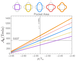
Figure 12: Different slopes of $S_{k}$ versus $\mu$ suggest the effective masses are different for the different orbits. The areas of $\alpha$, $\gamma$ and $\epsilon$ orbits are obtained from exact calculations of the Fermi surface, while for $\beta$ and $\delta$ orbits the areas are based on interpolation between the $\alpha$, $\gamma$ and $\epsilon$ orbits (shown as the thinner lines). The vertical line is the value of $\mu=-2.5306t_{a}$ chosen throughout our calculations.

While $\tilde{g}=0.87$ determines the effective mass of the electron pocket in a single layer and the central peak in the QO power spectrum, it is conceivable that the effective mass of the other viable semiclassical cyclotron orbits associated with the side peaks be different, as their enclosed areas are necessarily modified - Fig. 12 shows the enclosed areas of these orbits as the chemical potential is varied, and the effective mass extracted from the corresponding slope according to Eq. 28 is fully consistent with that obtained from the fit to QO amplitude versus $\theta$ angle of the magnetic field $\vec{B}$ in Fig. 6.

Appendix E Fourier Transform Analysis

Fast-Fourier transforms of finite data sets are known to introduce frequency ‘artifacts’ into power-spectrum plots. These artifacts originate in the choice of how the data is truncated. For example, a ‘boxcar’ function—whereby the signal is simply truncated at the start and end—introduces high-frequency components due to the sharp cutoffs at the data boundaries. Modern signal processing solves this through ‘apodization’, whereby the data is brought to zero in some way at the boundary. The choice of apodization function depends on what features in the data are of interest.

The data in Fig. 10 were processed using a Kaiser window, designed to resolve closely-spaced frequencies while suppressing side-lobes (at the expense of absolute amplitude determination, which was not important for this analysis). The weighting function $w$ for $N$ data points is defined as

$$w\left(n\right)=\frac{I_{0}\left(\pi\alpha\sqrt{1-\left(\frac{2n}{N-1}-1\right)^{2}}\right)}{I_{0}\left(\pi\alpha\right)},$$ (35)

where $I_{0}$ is the zeroth modified Bessel function of the first kind and $\alpha$ controls the roll-off of the weighting function (chosen to be 1.7 for this work). Fig. 13 shows the effect of such a windowing function on a signal and its Fourier transform.

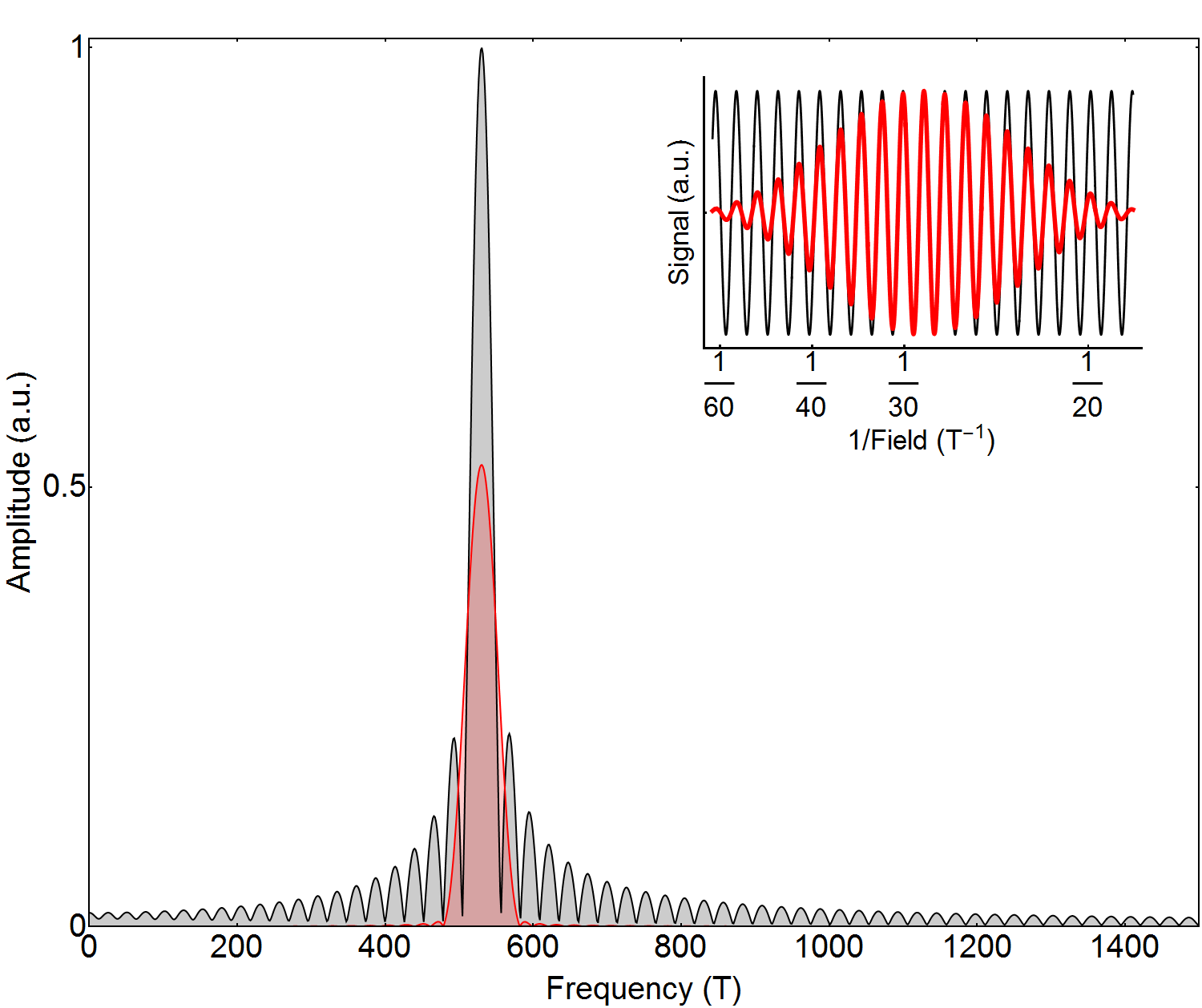
Figure 13: The inset shows two simulated data sets: one is apodized with a boxcar function (black), and the other uses equation 35 with $\alpha=1.7$ (red). The Fourier transform of the boxcar-apodized data shows multiple side-lobes introduced from the sharp cut-off. The data apodized with the Kaiser window has a main peak suppressed by about a factor of two, but with the first side-lobe suppressed 20 times more than that in the box-car data.

Simulated QO data is shown in the inset of Fig. 14. The data contains only the three central frequencies: 440, 530, and 620 T. Specifically, the function is

$$\tau=e^{-150/B}\left(\cos\left(\frac{2\pi~{}440}{B}-\pi\right)+\cos\left(\frac{2\pi~{}530}{B}-\pi\right)+\cos\left(\frac{2\pi~{}620}{B}-\pi\right)\right).$$ (36)

Note the lack of side-lobes near 350 and 710 T: this demonstrates that the $\alpha$ and $\epsilon$ peaks in Fig. 10 are not artifacts of the data analysis.

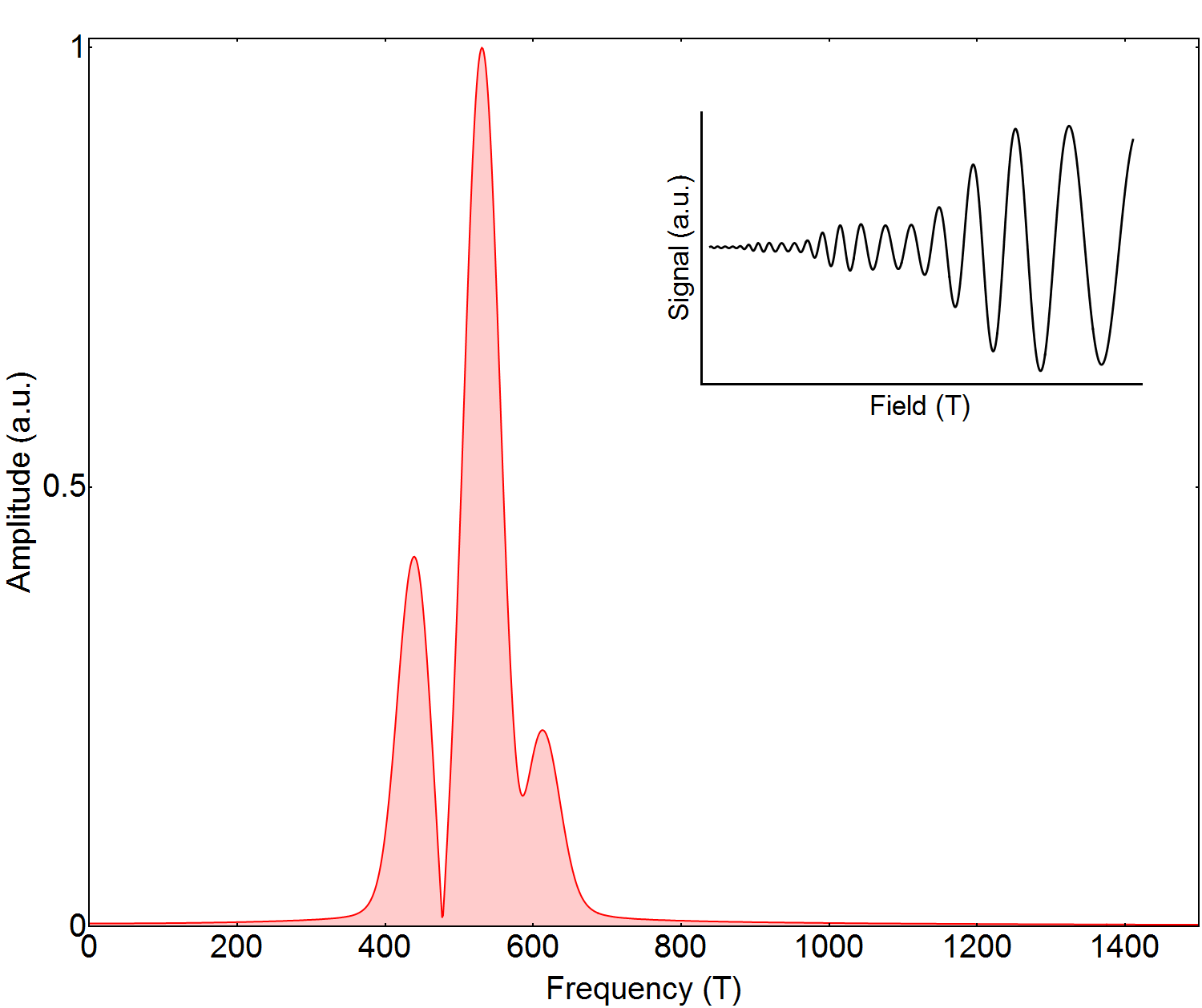
Figure 14: The inset shows simulated data from equation 36 before the window is applied. The Fourier transform uses the Kaiser window with $\alpha=1.7$—the same as the red curve in Fig. 13 and in Fig. 10 in the main text. Note that there are no extraneous side-lobes.

References

- Doiron-Leyraud et al. [2007] N. Doiron-Leyraud, C. Proust, D. LeBoeuf, J. Levallois, J. Bonnemaison, R. Liang, D. Bonn, W. Hardy, and L. Taillefer, Nature 447, 565 (2007).
- LeBoeuf et al. [2007] D. LeBoeuf, N. Doiron-Leyraud, J. Levallois, R. Daou, J.-B. Bonnemaison, N. Hussey, L. Balicas, B. Ramshaw, R. Liang, D. Bonn, et al., Nature 450, 533 (2007).
- Bangura et al. [2008] A. Bangura, J. Fletcher, A. Carrington, J. Levallois, M. Nardone, B. Vignolle, P. Heard, N. Doiron-Leyraud, D. LeBoeuf, L. Taillefer, et al., Physical review letters 100, 047004 (2008).
- Yelland et al. [2008] E. Yelland, J. Singleton, C. Mielke, N. Harrison, F. Balakirev, B. Dabrowski, and J. Cooper, Physical Review Letters 100, 047003 (2008).
- Vignolle et al. [2008] B. Vignolle, A. Carrington, R. Cooper, M. French, A. Mackenzie, C. Jaudet, D. Vignolles, C. Proust, and N. Hussey, Nature 455, 952 (2008).
- Audouard et al. [2009] A. Audouard, C. Jaudet, D. Vignolles, R. Liang, D. Bonn, W. Hardy, L. Taillefer, and C. Proust, Physical review letters 103, 157003 (2009).
- Sebastian et al. [2010] S. E. Sebastian, N. Harrison, P. Goddard, M. Altarawneh, C. Mielke, R. Liang, D. Bonn, W. Hardy, O. Andersen, and G. Lonzarich, Physical Review B 81, 214524 (2010).
- Singleton et al. [2010] J. Singleton, C. de La Cruz, R. McDonald, S. Li, M. Altarawneh, P. Goddard, I. Franke, D. Rickel, C. Mielke, X. Yao, et al., Physical review letters 104, 086403 (2010).
- Ramshaw et al. [2011] B. Ramshaw, B. Vignolle, J. Day, R. Liang, W. Hardy, C. Proust, and D. Bonn, Nature Physics 7, 234 (2011).
- Sebastian et al. [2012a] S. E. Sebastian, N. Harrison, R. Liang, D. Bonn, W. Hardy, C. Mielke, and G. Lonzarich, Physical review letters 108, 196403 (2012a).
- Sebastian et al. [2012b] S. E. Sebastian, N. Harrison, and G. G. Lonzarich, Reports on Progress in Physics 75, 102501 (2012b).
- Barišić et al. [2013] N. Barišić, S. Badoux, M. K. Chan, C. Dorow, W. Tabis, B. Vignolle, G. Yu, J. Béard, X. Zhao, C. Proust, et al., Nature Physics 9, 761 (2013).
- Sebastian et al. [2014] S. E. Sebastian, N. Harrison, F. Balakirev, M. Altarawneh, P. Goddard, R. Liang, D. Bonn, W. Hardy, and G. Lonzarich, Nature 511, 61 (2014).
- Sebastian and Proust [2015] S. E. Sebastian and C. Proust, Annu. Rev. Condens. Matter Phys. 6, 411 (2015).
- Ramshaw et al. [2015] B. Ramshaw, S. Sebastian, R. McDonald, J. Day, B. Tan, Z. Zhu, J. Betts, R. Liang, D. Bonn, W. Hardy, et al., Science 348, 317 (2015).
- Tranquada et al. [1994] J. Tranquada, D. Buttrey, V. Sachan, and J. Lorenzo, Physical review letters 73, 1003 (1994).
- Tranquada et al. [1995] J. Tranquada, B. Sternlieb, J. Axe, Y. Nakamura, and S. Uchida (1995).
- Fujita et al. [2004] M. Fujita, H. Goka, K. Yamada, J. Tranquada, and L. Regnault, Physical Review B 70, 104517 (2004).
- Howald et al. [2003] C. Howald, H. Eisaki, N. Kaneko, M. Greven, and A. Kapitulnik, Physical Review B 67, 014533 (2003).
- Hoffman et al. [2002] J. Hoffman, E. Hudson, K. Lang, V. Madhavan, H. Eisaki, S. Uchida, and J. Davis, Science 295, 466 (2002).
- Hanaguri et al. [2004] T. Hanaguri, C. Lupien, Y. Kohsaka, D.-H. Lee, M. Azuma, M. Takano, H. Takagi, and J. Davis, Nature 430, 1001 (2004).
- Fink et al. [2009] J. Fink, E. Schierle, E. Weschke, J. Geck, D. Hawthorn, V. Soltwisch, H. Wadati, H.-H. Wu, H. A. Dürr, N. Wizent, et al., Physical Review B 79, 100502 (2009).
- Laliberté et al. [2011] F. Laliberté, J. Chang, N. Doiron-Leyraud, E. Hassinger, R. Daou, M. Rondeau, B. Ramshaw, R. Liang, D. Bonn, W. Hardy, et al., Nature communications 2, 432 (2011).
- Chang et al. [2012] J. Chang, E. Blackburn, A. Holmes, N. Christensen, J. Larsen, J. Mesot, R. Liang, D. Bonn, W. Hardy, A. Watenphul, et al., Nature Physics 8, 871 (2012).
- Ghiringhelli et al. [2012] G. Ghiringhelli, M. Le Tacon, M. Minola, S. Blanco-Canosa, C. Mazzoli, N. Brookes, G. De Luca, A. Frano, D. Hawthorn, F. He, et al., Science 337, 821 (2012).
- Achkar et al. [2012] A. J. Achkar, R. Sutarto, X. Mao, F. He, A. Frano, S. Blanco-Canosa, M. Le Tacon, G. Ghiringhelli, L. Braicovich, M. Minola, et al., Phys. Rev. Lett. 109, 167001 (2012), URL http://link.aps.org/doi/10.1103/PhysRevLett.109.167001.
- Doiron-Leyraud et al. [2013] N. Doiron-Leyraud, S. Lepault, O. Cyr-Choiniere, B. Vignolle, G. Grissonnanche, F. Laliberté, J. Chang, N. Barišić, M. Chan, L. Ji, et al., Physical Review X 3, 021019 (2013).
- LeBoeuf et al. [2013] D. LeBoeuf, S. Krämer, W. Hardy, R. Liang, D. Bonn, and C. Proust, Nature Physics 9, 79 (2013).
- He et al. [2014] Y. He, Y. Yin, M. Zech, A. Soumyanarayanan, M. M. Yee, T. Williams, M. Boyer, K. Chatterjee, W. Wise, I. Zeljkovic, et al., Science 344, 608 (2014).
- Tabis et al. [2014] W. Tabis, Y. Li, M. Le Tacon, L. Braicovich, A. Kreyssig, M. Minola, G. Dellea, E. Weschke, M. Veit, M. Ramazanoglu, et al., Nature communications 5 (2014).
- Forgan et al. [2015] E. Forgan, E. Blackburn, A. Holmes, A. Briffa, J. Chang, L. Bouchenoire, S. Brown, R. Liang, D. Bonn, W. Hardy, et al., arXiv preprint arXiv:1504.01585 (2015).
- Chakravarty et al. [2001] S. Chakravarty, R. B. Laughlin, D. K. Morr, and C. Nayak, Phys. Rev. B 63, 094503 (2001), URL http://link.aps.org/doi/10.1103/PhysRevB.63.094503.
- Millis and Norman [2007] A. J. Millis and M. Norman, Physical Review B 76, 220503 (2007).
- Harrison and Sebastian [2011] N. Harrison and S. Sebastian, Physical Review Letters 106, 226402 (2011).
- Eun et al. [2012] J. Eun, Z. Wang, and S. Chakravarty, Proceedings of the National Academy of Sciences 109, 13198 (2012), eprint http://www.pnas.org/content/109/33/13198.full.pdf+html, URL http://www.pnas.org/content/109/33/13198.abstract.
- Harrison and Sebastian [2012] N. Harrison and S. Sebastian, New Journal of Physics 14, 095023 (2012).
- Lee [2014] P. A. Lee, Physical Review X 4, 031017 (2014).
- Allais et al. [2014] A. Allais, D. Chowdhury, and S. Sachdev, Nature communications 5 (2014).
- Wang and Chubukov [2014] Y. Wang and A. Chubukov, Physical Review B 90, 035149 (2014).
- Maharaj et al. [2014] A. V. Maharaj, P. Hosur, and S. Raghu, Phys. Rev. B 90, 125108 (2014), URL http://link.aps.org/doi/10.1103/PhysRevB.90.125108.
- Russo and Chakravarty [2015] A. Russo and S. Chakravarty, arXiv preprint arXiv:1504.03378 (2015).
- Briffa et al. [2015] A. Briffa, E. Blackburn, S. Hayden, E. Yelland, L. M.W., and E. Forgan, arXiv preprint arXiv:1510.02603 (2015).
- Harrison et al. [2015] N. Harrison, B. Ramshaw, and A. Shekhter, Scientific reports 5 (2015).
- Yao et al. [2011] H. Yao, D.-H. Lee, and S. Kivelson, Physical Review B 84, 012507 (2011).
- Riggs et al. [2011] S. C. Riggs, O. Vafek, J. Kemper, J. Betts, A. Migliori, F. Balakirev, W. Hardy, R. Liang, D. Bonn, and G. Boebinger, Nature Physics 7, 332 (2011).
- Doiron-Leyraud et al. [2015] N. Doiron-Leyraud, S. Badoux, S. R. de Cotret, S. Lepault, D. LeBoeuf, F. Laliberté, E. Hassinger, B. Ramshaw, D. Bonn, W. Hardy, et al., Nature communications 6 (2015).
- Wang and Chakravarty [2015] Z. Wang and S. Chakravarty, arXiv preprint arXiv:1509.00494 (2015).
- Andersen et al. [1995] O. Andersen, A. Liechtenstein, O. Jepsen, and F. Paulsen, Journal of Physics and Chemistry of Solids 56, 1573 (1995).
- Elfimov et al. [2008] I. Elfimov, G. Sawatzky, and A. Damascelli, Physical Review B 77, 060504 (2008).
- Fournier et al. [2010] D. Fournier, G. Levy, Y. Pennec, J. McChesney, A. Bostwick, E. Rotenberg, R. Liang, W. Hardy, D. Bonn, I. Elfimov, et al., Nature Physics 6, 905 (2010).
- Chakravarty et al. [1999] S. Chakravarty, H.-Y. Kee, and E. Abrahams, Physical review letters 82, 2366 (1999).
- Ioffe and Millis [1999] L. Ioffe and A. Millis, Science 285, 1241 (1999).
- Carlson et al. [2000] E. Carlson, D. Orgad, S. Kivelson, and V. Emery, Physical Review B 62, 3422 (2000).
- Zhang et al. [2015] Y. Zhang, A. V. Maharaj, and S. Kivelson, Physical Review B 91, 085105 (2015).
- Bergemann et al. [2003] C. Bergemann, A. Mackenzie, S. Julian, D. Forsythe, and E. Ohmichi, Advances in Physics 52, 639 (2003), ISSN 0001-8732.
- Chakravarty et al. [1993] S. Chakravarty, A. Sudbø, P. W. Anderson, and S. Strong, Science 261, 337 (1993).
- Gerber et al. [2015] S. Gerber, H. Jang, H. Nojiri, S. Matsuzawa, H. Yasumura, D. Bonn, R. Liang, W. Hardy, Z. Islam, A. Mehta, et al., arXiv preprint arXiv:1506.07910 (2015).
- Shoenberg [1984] D. Shoenberg, Magnetic oscillations in metals, Cambridge monographs on physics (Cambridge University Press, 1984), ISBN 9780521224802.
- Comin et al. [2015] R. Comin, R. Sutarto, F. He, E. da Silva Neto, L. Chauviere, A. Frano, R. Liang, W. Hardy, D. Bonn, Y. Yoshida, et al., Nature materials (2015).
- Chowdhury and Sachdev [2015] D. Chowdhury and S. Sachdev, Physical Review B 91, 115123 (2015).
- Chowdhury and Sachdev [2014] D. Chowdhury and S. Sachdev, Phys. Rev. B 90, 245136 (2014), URL http://link.aps.org/doi/10.1103/PhysRevB.90.245136.
- Hlobil et al. [2015] P. Hlobil, A. V. Maharaj, P. Hosur, M. Shapiro, I. Fisher, and S. Raghu, Physical Review B 92, 035148 (2015).