Electromagnetically controlled multiferroic thermal diode

Abstract

We propose an electromagnetically tunable thermal diode based on a two phase multiferroics composite. Analytical and full numerical calculations for prototypical heterojunction composed of Iron on Barium titanate in the tetragonal phase demonstrate a strong heat rectification effect that can be controlled externally by a moderate electric field. This finding is of an importance for thermally based information processing and sensing and can also be integrated in (spin)electronic circuits for heat management and recycling.

Introduction. A diode, i.e., a device that controls the electrical current flow direction, is an integral part of everyday electronics. The sonic counterpart governs the propagation of mechanical vibrations and has wide-ranging applications in acoustics, medical sensing, and in heat management. Acoustic (sound waves) diodes were recently demonstrated N13 ; N14 . Thermal diodes are more challenging, however. Even though heat and sound are of phononic nature, the frequency range of the latter is typically in the range of kHz-GHz (hypersound). Heat, on the other hand, is mediated by a broad spectrum of THz vibrations. Controlling heat diodes is therefore more delicate, but on the plus side the relevant scale for material structuring is on the nanometer allowing so, as shown below, to exploit the marked achievements of nanotechnology in tuning the material compositions and the associated electric, magnetic and optical properties. Applications are diverse. For instance, in spintronics it was shown that a thermal gradient may generate a direction-dependent spin current that can be utilized for information handling SSE . Such thermal magnetic diodes would add so an essential element towards thermally based spintronic circuits. Generally, substantial research was devoted in recent years to phononic-based diodes 12 ; 13 ; 14 ; 15 ; 16 . Our aim here is to add a new facet, namely the external control of thermal diodes via electric and/or magnetic fields. In view of an experimental implementation we consider a well-tested system composed of two-phase multiferroic (MF), i.e., a ferroelectric (FE) structure interfacially coupled to a ferromagnet (FM). The interfacial coupling renders the transmission and conversion of magnetic excitations into ferroelectric ones. The thermal energy in the proposed multiferroic thermal diode is carried by elementary excitations of electric polarization and magnetization (rather than by vibrational excitation in conventional thermal diode) both of which are susceptible to external electric or magnetic fields. As shown below, the performance of the thermal diode is then controllable electromagnetically. Multiferroics, in general, are intensively investigated in view of a variety of applications in electronics and sensing 1 ; 2 ; 3 ; 4 ; 5 ; 6 ; 7 ; 8 ; 9 ; 10 . Thus, the current study augments these applications with the possibility of a controlled heat recycling.

Multiferroic thermal diode. The physics of a thermal diode is a resonance phenomenon 16 relying on the overlapping of the temperature-dependent power spectra of thermal excitations (mediated by polarization, magnetization, and other type of excitations) of the two different diode segments. In addition, the dependence of frequency on the oscillation amplitude, i.e., the nonlinear nature of excitations is a key factor. A perfect thermal conductance hints on power spectra overlapping. Our aim here is to demonstrate that thermal bias applied on the edges of MF thermal diode generates a heat flux that can be rectified and controlled by temperature, electric field and interface ME coupling. To this end, we assume that the FM part of the thermal diode is a normal ferromagnetic metal (e.g., Fe). As a prototypical FE we employ BaTiO₃. For this experimentally realized composite an interfacial magneto electric coupling 6 ; 17 was demonstrated. The ferroelectric dynamics of BaTiO₃ is captured by the Ginzburg-Landau-Devonshire (GLD) potential 18 valid at temperatures $\sim$280-400 [K] (tetragonal phase) in which case the polarization switches bidirectionally. In the spirit of a coarse-grained approach, the FE order parameter is discretized into $N$ cells (also called sites) each with a size of 1 nm PiLe04 . The coarse-grained polarization at site $n$ is referred by $p_{n}$. In the tetragonal phase, realized also at room temperature, we have one component (Ising type) polarization vector $\vec{p}_{n}=\big{(}0,0,p_{n}^{z}\big{)},~{}~{}n=1,...N$ (here $n$ is the site number) entering the ferroelectric free energy functional 18 . In the context of thermal diode an important fact is that, by applying an external electric field, the temperature range of the tetragonal phase can be extended Wang ; Fesenko . Taking the general cubic paraelectric phase as a reference, we performed numerical calculations which turned out to be in line with the experimentally determined phase diagram Wang . The result of our calculations is shown in Fig. 1. As we see by applying an electric field with an amplitude E=100 [MV/m] the lower limit of the tetragonal phase is reduced from T=280 [K] to the T=200 [K] while the upper limit of the tetragonal phase exceeds T=500[K].

$\begin{array}[]{c}\includegraphics[width=227.62204pt]{t_e_phase_diagram.eps}\end{array}$

Figure 1: Full-Simulations of BaTiO₃ phase diagram based on 8-order temperature-dependent potentialWang .

For FM we employ the well-established classical Heisenberg model to describe transversal excitations of the coupled (coarse grained) magnetic moment $\vec{M}_{n}$ at site $n$. Experiments done for the different materials Hess evidence the dominant role of magnons for the thermal heat conductance at relatively high temperatures $T>20$ [K]. The relevance of magnons to thermal heat conductance was also confirmed by the spin Seebeck effect Xiao . The multiferroic interaction between the interfacial FE cell (with $p_{N}$) and the adjacent FM cell (with $M^{z}_{N+1}$) is described by the $\mathcal{PT}$ invariant term $V_{ME,m}=-g_{m}\left(p_{N}M^{z}_{N+1}\right)^{m}$, the form and the origin of which we discussed at length recently and contrasted with experimental findings jia14 ; 19 ; 20 ; 21 ; 22 ; 23 ; 24 ; 11 . Here we account for the linear ($V_{ME,1}$) and quadratic ($V_{ME,2}$) terms (for low energy excitations, higher order terms are less relevant to the effects studied here). $g_{m}$ is the magnetoelectric coupling constant. The total Hamiltonian of the composite reads $H=H_{p}+H_{s}+V_{ME}$, where $H_{p}=\sum\limits_{n=1}^{N}\big{[}\frac{1}{2}\big{(}\frac{dp_{n}}{dt}\big{)}^{2}-\frac{\alpha^{EF}}{2}p_{n}^{2}+\frac{\beta^{EF}}{4}p_{n}^{4}+\frac{1}{2}\big{(}p_{n+1}-p_{n})^{2}-Ep_{n}\big{]}$ is the FE Hamiltonian and $H_{S}=\sum\limits_{k=N+1}^{M}\big{(}-J\vec{M}_{k}\vec{M}_{k+1}-D\big{(}M_{k}^{z}\big{)}^{2}-BM_{k}^{z}\big{)}$ is the FM Hamiltonian. Unless otherwise stated, we use dimensionless units (d.u.). For values of all parameters in conventional units as used experimentally we refer to the Appendix. The effect of the applied thermal bias can be described by a stochatic field added to the effective electric field in time-dependent GLD equation Klotins . The microscopic mechanism for the emergence of noise in FE is based on phonons. Thermally activated phonons lead to electric dipole vibrations that can be captured by a random electric field. Experimentally, thermally activated polarization switches at much lower field strengths than predicted by GLD phenomenologyViehland (without including noise). The equations of motion for the polarization $p_{n}$ read 11

$$\begin{split}\frac{dp_{n}}{dt}=&q_{n}\\ \frac{dq_{n}}{dt}=&\alpha^{FE}p_{n}-\beta^{FE}p^{3}_{n}-(2p_{n}-p_{n+1}-p_{n-1})+E\\ &+g_{1}M^{z}_{1}\delta_{nN}+2g_{2}p_{n}\big{(}M^{z}_{1}\big{)}^{2}\delta_{nN}-\gamma_{n}q_{n}\delta_{1n}\\ &+\delta_{1n}\xi_{n},\quad\quad n=1,\cdots N.\end{split}$$ (1)

Here $\alpha^{FE}$, $\beta^{FE}$ are the kinetic parameters of the GLD potential, $E$ is the amplitude of the external electric field, $g_{1}M^{z}_{1}\delta_{nN}+2g_{2}p_{n}\big{(}M^{z}_{1}\big{)}^{2}\delta_{nN}$ is the contribution from the ME coupling, and the last two terms in (1) describe the influence of the thermal bias applied on the edges of the FE chain. The correlation function of the random noise $\xi_{n}$ is related to the kinetic constant $\gamma_{n}$ and the thermal energy $k_{B}T$ via the Einstein relation

$$\langle\xi_{m}(t)\xi_{m}(t^{\prime})\rangle=2\gamma_{m}T_{m}\delta(t-t^{\prime}),\quad m=1,\cdots N.$$ (2)

The magnetization dynamics of the FM part is governed by a set of coupled polarization-dependent LLG equations as follows

$$\frac{d\vec{M}_{k}}{dt}=-\frac{1}{1+\alpha_{k}^{2}}\vec{M}_{k}\times\left(\vec{B}^{eff}_{k}+\alpha_{k}\vec{M}_{k}\times\vec{B}^{eff}_{k}\right).$$ (3)

Here $\alpha_{k}=\alpha\delta_{kM}$ and $\vec{B}^{eff}_{k}$ are the total effective (electric polarization-dependent) magnetic field acting on the k-th magnetic moment $k\in[N+1,M]$

$$\begin{split}\vec{B}^{eff}_{k}=&\vec{i}_{z}B+J\left(\vec{M}_{k-1}+\vec{M}_{k+1}\right)+\vec{i}_{z}2DM^{z}_{k}\\ &+\vec{i}_{z}g_{1}p_{N}\delta_{k\,{N+1}}+\vec{i}_{z}2g_{2}p_{N}^{2}M^{z}_{k}\delta_{k\,{N+1}}+\delta_{kM}\vec{\eta}_{k}.\end{split}$$ (4)

$\vec{i}_{z}$ is a unit vector along the magnetization direction of the undistorted FM which we choose as the $z$ direction. The effective magnetic field (Eq. (4)) contains a deterministic contribution from the external magnetic field $\vec{i}_{z}B$, and the contributions from exchange $J\left(\vec{M}_{k-1}+\vec{M}_{k+1}\right)$ and magnetic anisotropy $\vec{i}_{z}2DM^{z}_{k}$. Due to its interfacial nature the magnetoelectric coupling $\vec{i}_{z}g_{1}p_{N}\delta_{k\,{N+1}}+\vec{i}_{z}2g_{2}p_{N}^{2}M^{z}_{k}\delta_{k\,{N+1}}$ acts on the interfacial FM and FE cells only. The random magnetic field $\vec{\eta}_{k}$ enters the dynamic of the edge cells only (thermal bias is applied at the end of the FM chain), while the heat propagation through the structure is evaluated self-consistently. The random magnetic field $\vec{\eta}_{k}$ is quantified via the correlation function

$$\langle\eta^{i}_{k}(t)\eta^{j}_{k}(t^{\prime})\rangle=2\alpha_{k}T_{k}\delta_{ij}\delta(t-t^{\prime}).$$ (5)

Here $i$ and $j$ define the Cartesian components of the random magnetic field, $k$ numbers the cell, and $T_{k}$ is the cell-dependent local temperature. $\alpha_{k}$ is the dimensionless Gilbert damping constant. Values of the FM and FE parameters used in the calculations are given in the TABLE I in the Appendix. Following the continuity equation for the local energy and the equipartition theorem, the heat current and the temperature profile can be evaluated self-consistently 16 . In particular, the expression for the heat current in the FE part reads $J^{H}_{k}=-\langle\dot{p}_{k}(p_{k+1}-p_{k})\rangle$. The time derivative of the polarization $\dot{p}_{k}$ plays the role of a canonical momentum. In the FE part the local (site dependent) temperature follows from its relation to the average local kinetic energy 16 which in our scaled units implies $T_{k}=\left(\frac{dp_{k}}{dt}\right)^{2}$. We note that average here means long time average which in numerical simulations is implemented as ensemble average. We derive the expression for the local heat current in the FM part by using Heisenberg equation of motion $\frac{\partial h_{k,k+1}}{\partial t}=i\left[H_{S},h_{k,k+1}\right]$. Here $H_{S}=-J\sum_{k}\vec{M}_{k}\cdot\vec{M}_{k+1}-D\sum_{k}\left(M^{z}_{k}\right)^{2}-B\sum_{k}M^{z}_{k}$ is the Hamiltonian of the system and $h_{k,k+1}=-J\vec{M}_{k}\cdot\vec{M}_{k+1}-D\left(M^{z}_{k}\right)^{2}-BM^{z}_{k}$ is the local Hamiltonian. After straightforward calculations the heat current in the FM part is obtained as

$$\begin{split}J^{H}_{k}=&i\left[h_{k+1,k},h_{k,k-1}\right]\\ =&2DJ\left(M^{x}_{k+1}M^{y}_{k}M^{z}_{k}-M^{x}_{k}M^{y}_{k+1}M^{z}_{k}\right)\\ &+DB\left(M^{y}_{k}M^{x}_{k+1}-M^{x}_{k}M^{y}_{k+1}\right)\\ &-J^{2}\left(M^{x}_{k-1}M^{y}_{k}M^{z}_{k+1}-M^{x}_{k-1}M^{y}_{k+1}M^{z}_{k}\right)\\ &-J^{2}\left(M^{x}_{k+1}M^{y}_{k-1}M^{z}_{k}-M^{x}_{k}M^{y}_{k-1}M^{z}_{k+1}\right)\\ &-J^{2}\left(M^{x}_{k}M^{y}_{k+1}M^{z}_{k-1}-M^{x}_{k+1}M^{y}_{k}M^{z}_{k-1}\right).\end{split}$$ (6)

The equilibrium temperature $T_{k}$ is evaluated self-consistently via the relation $M^{\|}_{k}=L\left(\frac{\vec{M}_{k}\cdot\vec{B}^{eff}_{k}}{T_{k}}\right)$, where $L(...)$ is the Langevin function and $M^{\|}_{k}$ is the component of magnetization vector parallel to the effective field $\vec{B}^{eff}_{k}$.

$\begin{array}[]{c}\includegraphics[width=216.81pt]{temperature_effect.eps}\\ \includegraphics[width=216.81pt]{temperature-heat_profiles.eps}\end{array}$

Figure 2: a) Diode heat current under different edge temperatures. The multiferroic diode includes 50 FE cells (from 1 to 50) and 50 FM cells (from 51 to 100). In dimensional units, the applied electric and magnetic fields are $E=1.74$ d.u. and $B=0.0$ d.u. and FE-FM coupling coefficients are $g_{1}=g_{2}=-1$ d.u.. Other employed parameters and reduced unit coefficients are tabulated in TABLE I in the Appendix. b) Heat current profile for forward temperature bias ($\Delta=1.4$), reverse temperature bias ($\Delta=-1.4$) and $T_{0}=400$ K. c) Temperature profiles for forward temperature bias ($\Delta=1.4$) and reverse temperature bias ($\Delta=-1.4$), $T_{0}=400$ K. In the both cases temperature formed in the FE part corresponds to the tetragonal phase.

Interface effect and heat rectification.- An important element of the thermal diode is the interface thermal resistance (ITR), usually referred to as the asymmetric Kapitza resistance 16 as it quantifies the asymmetry in interfacial resistance. We will consider the cases in which the hot thermal bath is applied to the FE part $T_{FE}>T_{FM}$ and to the FM part $T_{FE}<T_{FM}$ respectively. Inverting the sign of the thermal bias for a constant temperature difference $\Delta T=\mid T_{FE}-T_{FM}\mid$ drastically changes the heat flux $J_{+}\neq J_{-}$ and the resistance $R_{+}=\Delta T/J_{+}$, $R_{-}=\Delta T/J_{-}$. The ratio between the two different resistance $R_{+}/R_{-}$ measures the rectification effect. The rectification effect of the MF diode stems from the overlapping of the spectra of the FE and FM subsystems. The frequency of the linear excitations in FM $\omega_{FM}$ is set by the anisotropy constant $\approx 2D$ 11 . The applied electric field substantially modifies the frequency of linear excitations in the FE part, $\omega_{FE}$. Basically the electric field shifts the minimum of the GLD potential derived from the relation $\partial_{p}H_{p}=0$. In the limit of a weak coupling between the dipoles, FE frequency takes the form $\omega_{FE}\big{(}E\big{)}=\big{(}4\alpha^{FE}\cos^{2}\big{[}\cos^{-1}\big{(}\frac{3|E|}{2\alpha^{FE}}\sqrt{\frac{3\beta^{FE}}{\alpha^{FE}}}\big{)}/3\big{]}-\alpha^{FE}\big{)}^{1/2}$. So, the correction in the FE frequency $\Delta\omega_{FE}=\omega_{FE}\big{(}E\big{)}-\omega_{FE}\big{(}0\big{)}$ is even in the electric field (for more details we refer to the Appendix). Therefore, the heat current is symmetric with respect to the change of the electric field’s sign $E\rightarrow-E$. On the other hand, maximal heat conductance occurs when FM and FE frequencies $\omega_{FM}\approx\omega_{FE}\big{(}0\big{)}+\Delta\omega_{FE}$ match. Thus, the electric field can be utilized to enhance the heat current. From the frequency matching condition and for the parameters listed in the TABLE I in the appendix, we obtain an estimation of the optimum electric field as $|E|=|\frac{2\alpha^{FE}}{3}\sqrt{\frac{\alpha^{FE}}{3\beta^{FE}}}\cos\big{(}\frac{3}{2}\cos^{-1}\big{(}\frac{4D^{2}-\alpha^{FE}}{2\alpha^{FE}}\big{)}\big{)}|=0.1$ (d.u.). In conventional units this corresponds to an electric field of $E=3.4\times 10^{4}[V/cm]$. Increasing the electric field strength results in a mismatch of FE and FM spectra and hence a decrease of the heat current. This analytical estimation is confirmed by full numerical calculations as well (Fig. 3 below). Interface ME coupling leads to a small shift between analytically estimated and numerically calculated values of the optimum electric field. However, we see prominent maximum in the heat current for optimal electric field.

Temperature effects on MF diode.- We implemented full numerical simulations for a MF thermal diode consisting of 50 dipolar and 50 magnetic cells. Calculations are also done for larger system (not shown) up to 500 dipolar and 500 magnetic cells and we did not observe significant size effects. Of a special interest is the rectification effect. We present the edge temperatures in the following form: $T_{1}=T_{0}+T_{S}\Delta,~{}~{}T_{M}=T_{0}-T_{S}\Delta$ where $M$ is the total number of sites. Thus, the difference between the edges temperatures is $T_{1}-T_{M}=2T_{S}\Delta$. Inverting the thermal bias simply means $\Delta\rightarrow-\Delta$. The heat current as a function of $\Delta$ for different values of $T_{0}$ is shown in Fig. 2a. We observe that at larger temperature $T_{0}$ the asymmetry becomes stronger. The uniform heat flux through the system [see Fig. 2b] affirms that the system is in the nonequilibrium steady state. On the other hand due to the different heat capacities of the FE and FM systems and the different heat exchange rates with the environment, the temperatures formed self-consistently in the FE and FM parts are different. In the case of an applied positive thermal bias the heat flux $J_{+}=0.8$ d.u. while for a negative thermal bias the flux reaches $J_{-}=2.5$ d.u. and therefore $R_{-}/R_{+}<1$. This rectification is also characterized by distinct temperature profiles for opposite thermal differences [see Fig.2c].

Electric field effect on the MF diode.- The heat current as a function of $\Delta$ is displayed in Fig. 3. We note that the change of the sign of $\Delta$ corresponds to the inverted thermal bias. Besides, we consider different amplitudes of the applied electric field, in order to see whether an electric field may enhance the heat rectification effect. As shown in Fig. 3a the rectification effect becomes stronger upon increasing the electric field strength. However, the role of the electric field is not trivial. As shown in the inset, there is an optimum electric filed for which the asymmetry of diode is maximal. The optimal value $E\approx 0.75$ d.u. corresponds to the frequency matching condition $\omega_{FM}\approx\omega_{FE}\big{(}0\big{)}+\Delta\omega_{FE}$ and is quite close to the analytical value that we estimated above without interface ME coupling. Further increasing the electric field destroys the spectra-matching condition and reduces the heat current. Magnetic field $B$ however monotonically decreases the heat flux as shown in Fig. 3b. This is due to the fact that the stronger the magnetic field the stiffer the magnetization in the FM part, which suppresses the energy transport.

$\begin{array}[]{c}\includegraphics[width=216.81pt]{electric_filed_effect.eps}\\ \includegraphics[width=216.81pt]{magnetic_filed_effect.eps}\end{array}$

Figure 3: a) Heat current versus the biased temperature difference in the MF diode for different values of electric filed ($E$). The MF diode includes 50 FE cells (from 1 to 50) and 50 FM cells (from 51 to 100). FE-FM coupling coefficients are $g_{1}=g_{2}=-1$ d.u.. Other employed parameters are tabulated in TABLE I in the Appendix. The inset shows the dependency of heat current on electric field for $\Delta=\pm 0.6$. b) The same but for magnetic field. The electric field increases the heat current reaching a maximum at the optimal electric field. In contrast, the magnetic field decreases the heat current.

Interfacial ME coupling effects on the MF diode.- Fig. 4 shows the heat current as a function of the interfacial ME coupling constant ($g=g_{1}=g_{2}$ d.u.) for forward and reverse biases, respectively. Without magnetoelectric coupling the heat current across the MF diode diminishes. In the range of $g=[-1,0]$ d.u. the rectifying effect is magnified monotonically when increasing $g$ from $0$ to $-1$ and the maximum rectifying effect (asymmetry) is achieved at $g=-1$ d.u., which is the value we have used in all other simulations. Surprisingly, a different picture emerges in the positive range of $g=[0,0.8]$ d.u., where a large coupling strength near $0.8$ d.u. deteriorates the heat current in both directions. The optimal transport and rectification are achieved at an intermediate strength of $g$ around $0.4$ d.u. This distinct response upon the sign change of the coupling constant can be traced back to the fact that such a change influences the ground state of the polarization and the magnetization configurations of the MF diode system. For a different sign of the coupling constant, slightly different configurations correspond to the ground state with a minimal energy. For the explicit form of the interface coupling term $V=-g\big{(}P_{N}M_{1}^{z}\big{)}-g\big{(}P_{N}M_{1}^{z}\big{)}^{2}$ we find that the positive coupling constant $g>0$ favors large values of the magnetization component $M_{1}^{z}$. Aligning the magnetic moment along the $z$ axis naturally decreases the current, which is consistent with the picture of the inset of Fig. 3b. In the case of a negative $g<0$ the situation is different. A small $M_{1}^{z}$ means a larger transversal components and this enhances the current.

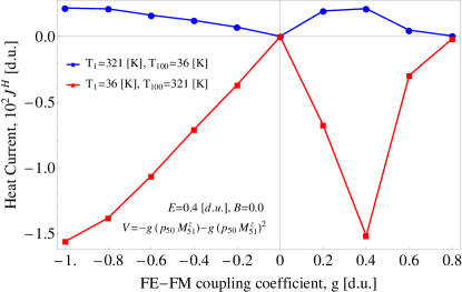
Figure 4: Heat current in the MF diode versus FE-FM coupling coefficients ($g=g_{1}=g_{2}$ d.u.) for forward and reverse temperature biases. The MF diode includes 50 FE cells (from 1 to 50) and 50 FM cells (from 51 to 100). The applied electric and magnetic fields are $E=0.4$ d.u. and $B=0.0$ d.u.. Other employed parameters are tabulated in TABLE I in the Appendix.

In summary, we proposed and demonstrated a thermal diode based on a two phase multiferroic composite. The heat transfer through it can be rectified and controlled by a thermal bias and an electromagnetic field. In particular, the external electric field applied to the ferroelectric part of the multiferroic thermal diode can substantially enhance the heat conductance and the rectification. On the other hand we found that an applied magnetic field decreases the heat current. We demonstrated and discussed how the interfacial magnetoelectric coupling influences the thermal diode operation in a dynamical way. In view of contemporary advances in engineering composite multiferroic structures, the present findings are potentially interesting for applications, e.g., as elements in thermal switches and thermal memories 24 , and thermal management via multifunctional caloric materials Moya .

I Appendix

Definitions of the dimensionless units. The total energy of the ferroelectric subsystem $H_{P}$ as a function of the coarse-grained polarization $P_{n}$ and corresponding equations of motion read: $H_{P}=\sum_{n=1}^{N}\frac{\alpha_{0}}{2}\dot{P}_{n}^{2}-\frac{\alpha_{1}}{2}P_{n}^{2}+\frac{\alpha_{2}}{4}P_{n}^{4}+\frac{\kappa}{2}(P_{n+1}-P_{n})^{2}-EP_{n}$, and $\alpha_{0}\ddot{P}_{n}=\alpha_{1}P_{n}-\alpha_{2}P_{n}^{3}-\kappa(-(P_{n+1}-P_{n})+(P_{n}-P_{n-1}))+E$. This equation is normalized by introducing $p_{n}=P_{n}/P_{0}$, $E\rightarrow E/kP_{0}$. Dividing both parts by $\kappa$ leads to the new reduced time $t^{\prime 2}=t^{2}/(\kappa/\alpha_{0})$ or $t^{\prime}=\omega_{0}t$, where $\omega_{0}=\sqrt{\frac{\kappa}{\alpha_{0}}}$. Finally, we obtain the equation for the polarization dynamics in fully dimensionless units for $n\neq N$ (see Eq. (1)) with $\alpha^{FE}=\alpha_{1}/\kappa$, $\beta^{FE}=\alpha_{2}P^{2}_{0}/\kappa$.

Time scales. The frequency of oscillations associated with the mode-plasma frequency $\omega_{0}$ is higher than the inverse relaxation time $\alpha_{1}/\gamma_{\nu}$RiHa98 (s. TABLE 1). The overdamped case yields the Landau-Khalatnikov equation LaKh54 employed for modeling the polarization hysteresis RiHa98 ; PiLe04 ). An overview over the real parameters and their dimensionless counterparts for the ferroelectric subsystem is given in TABLE 1. The time scale within the present calculations is set by the frequency $\omega_{0}$ which is related to the mode-plasma frequency or the fast oscillations (also known as ”eigen-displacements” or Slater modes 21 ) of the $Ti$-atom in BaTiO₃. Ab-initio calculations for BaTiO₃ GhCo99 yield $\Omega_{Slater}=1519$ [cm^-1]=$286\cdot 10^{12}$ [s^-1], the experimental values differ slightly at $T=300$ [K] yielding $\Omega_{Slater}=1628$ [cm^-1], as given in Ref. SeGe80 . Finally, one can also estimate the mode-plasma frequency as Cao94 $\omega_{0}=Z^{*}_{\mathrm{Ti}}e\sqrt{\frac{1}{m_{Ti}\varepsilon_{0}a^{3}_{0}}}$, where $Z^{*}_{\mathrm{Ti}}=7$, given in Ref. 18 is the Born effective charge and $m_{Ti}=47.9$ [amu]=$79,5\cdot 10^{-27}$ [kg]. For the displacement of several Angstrom $\omega_{0}\approx 100\cdot 10^{12}$ [s^-1]. In our numerical calculations the dimensionless time scales, however, with the prefactor of $\omega_{0}/(2\pi)$, therefore we arrive at the approximate value of $\sim 10^{12}$ [Hz].

Parameters of the FM part. For FM part employ the Landau-Lifshitz-Gilbert equation of motionLaLi35 ; Gilb55 (see Eq. (3)) Bulk parameters for Fe: anisotropy strength $K_{1}\approx 5.0\cdot 10^{4}$ [J/m³] given in Ref. 22 , the saturation magnetization $M_{S}=1.7\cdot 10^{6}$ [A/m] given in Ref. 22 . The Larmor (precessional) frequency in the local anisotropy field scales as $\omega_{prec}/(2\pi)=\gamma 2K_{1}/(M_{S})\approx 8\cdot 10^{9}$ [Hz], frequency associated with the relaxation scales as $\omega_{rel}/(2\pi)=\alpha_{FM}\omega_{prec}/(2\pi)\approx 0.08\cdot 10^{9}$ [Hz]. The autocorrelation function of the thermal fields in FE and FM part in standard units are given as $\langle\xi_{k}(t)\xi_{k}(t^{\prime})\rangle=\frac{2k_{B}\gamma_{\nu}}{a_{FE}^{3}}T_{k}\delta(t-t^{\prime})$ and $\langle\eta^{i}_{k}(t)\eta^{j}_{k}(t^{\prime})\rangle=\frac{2k_{B}\alpha_{FM}}{\gamma M_{\mathrm{S}}a_{FM}^{3}}T_{k}\delta_{kM}\delta_{ij}\delta(t-t^{\prime})$ where $T_{k}$ is the site-dependent local temperature in Kelvin.
Shift of ferroelectric frequency. We consider one unit cell in the FE Hamiltonian: $\displaystyle H_{P}=\frac{1}{2}\dot{p}^{2}-\frac{\alpha^{FE}}{2}p^{2}+\frac{\beta^{FE}}{4}p^{4}-Ep$ Equilibrium properties are given by the condition $\partial H_{p}=0$. After solving cubic equation we obtain : $p_{1}^{(0)}=\frac{2}{\sqrt{3}}\sqrt{\frac{\alpha^{FE}}{\beta^{FE}}}\cos\left(\frac{\theta}{3}\right)$, $p_{2}^{(0)}=\frac{2}{\sqrt{3}}\sqrt{\frac{\alpha^{FE}}{\beta^{FE}}}\cos\left(\frac{\theta}{3}+\frac{2\pi}{3}\right)$ and $p_{3}^{(0)}=\frac{2}{\sqrt{3}}\sqrt{\frac{\alpha^{FE}}{\beta^{FE}}}\cos\left(\frac{\theta}{3}+\frac{4\pi}{3}\right)$. Here $\theta=\arccos\left(\frac{3E}{2\alpha^{FE}}\sqrt{\frac{3\beta^{FE}}{\alpha^{FE}}}\right)$ and minimum of the energy reads: $H\left(p_{1,2}^{(0)}(E)\right)=-\frac{(\alpha^{FE})^{2}}{4\beta^{FE}}\pm\sqrt{\frac{\alpha^{FE}}{\beta^{FE}}}E$. As we see if $E>0$ then minimum of the energy corresponds to the solution $p_{1}^{(0)}(E)$ while if $E<0$ then energy minimum corresponds to the solution $p_{2}^{(0)}(E)$. Taking into account fact that system is even in electric field we express minimum of the energy in the form valid for the both $E>0$ and $E<0$ cases: $H\left(p_{1,2}^{(0)}(E)\right)=-\frac{(\alpha^{FE})^{2}}{4\beta^{FE}}-\sqrt{\frac{\alpha^{FE}}{\beta^{FE}}}|E|$.

Table 1: Parameters of an unstrained bulk BaTiO₃-single crystalHlMa06 ; MaHl08 ; SeDa06 ; HlPe06 and bulk bcc-Fe22 (p. 385).

parameter	SI units	dimensional unit (d.u.)
$P_{0}$	0.265 [C/m2]	$p_{n}=P_{n}/P_{0}$
$\alpha_{1}$	$2.770\cdot 10^{7}$ [V$\cdot$m/C]	$\alpha^{FE}=\frac{\alpha_{1}}{\kappa}\approx 0.213$
$\alpha_{2}$	$1.7\cdot 10^{8}$ [V$\cdot$m5/C3]	$\beta^{FE}=\frac{\alpha_{2}P_{0}^{2}}{\kappa}\approx 0.0918$
$\gamma_{\nu}$	$2.5\cdot 10^{-5}$ [V$\cdot$m$\cdot$s/C]	$\gamma_{m}=\frac{\gamma_{\nu}\omega_{0}}{\kappa}\approx 0.192$
$a_{FE}$	$1.02\cdot 10^{-9}$ [m]	-
$\kappa$	$1.3\cdot 10^{8}$ [V$\cdot$m/C]	1
$E$	parameter [V/m]	$E\rightarrow\frac{1}{\kappa P_{0}}E\approx 3.4\times 10^{7}E$
$T$	parameter [K]	$T\rightarrow\frac{k_{B}}{\kappa P_{0}^{2}a_{FE}^{3}}T\approx 1.4\times 10^{-3}T$
$J$	- [Joule/s]	$J\rightarrow\frac{1}{\kappa P_{0}^{2}\omega_{0}a_{FE}^{3}}J\approx 10^{8}J$
$M_{\mathrm{S}}$	$1.71\cdot 10^{6}$ [A/m]	$\vec{s}_{k}=\vec{M}_{k}/M_{S}=\left(\vec{S}_{k}/S\right)$
$\gamma$	$1.76\cdot 10^{11}$ [(T$\cdot$s)-1]	-
$a_{FM}$	$1.0\cdot 10^{-9}$ [m]	-
$\mu_{S}=M_{S}a^{3}_{\mathrm{FM}}$	$1.71\cdot 10^{-21}$ [J/T]	-
$\alpha_{FM}$	$1.0$	-
$K_{1}$	$2.0\cdot 10^{6}$ [J/m3]	$D=\frac{\gamma a_{FM}^{3}K_{1}}{\omega_{0}\mu_{S}}=0.206$
$A$	$2.1\cdot 10^{-11}$ [J/m]	$J=\frac{\gamma a_{FM}A}{\omega_{0}\mu_{S}}=2.16$
$B$	parameter [T]	$B\rightarrow\frac{\gamma}{\omega_{0}}B\approx 0.17B$
$T$	parameter [K]	$T\rightarrow\frac{k_{B}\gamma}{\omega_{0}\mu_{S}}T\approx 1.4\times 10^{-3}T$
$J$	- [Joule/s]	$J\rightarrow\frac{\gamma}{\omega_{0}^{2}\mu_{S}}J\approx 10^{8}J$

In order to evaluate dependence of the FE frequency on the applied external electric field we expand Hamiltonian $H_{p}$ in the vicinity of the equilibrium points. In the equation of motion governed by linearized Hamiltonian $\ddot{p}=-\left(-\alpha^{FE}+3\beta^{FE}p_{0}^{2}\right)p+E$ enters electric field dependent frequency: $\omega^{2}_{p}(E)=\left(-\alpha^{FE}+3\beta^{FE}p_{0}^{2}\right)$. Considering small electric field $E$ in the first order approximation from $p_{1,2,3}^{(0)}$ we obtain: $\omega_{p}(E>0)=\sqrt{2\alpha^{FE}}+\frac{3E}{2\alpha^{FE}}\sqrt{\frac{\beta^{FE}}{2}}$, $\omega_{p}(E<0)=\sqrt{2\alpha^{FE}}-\frac{3E}{2\alpha^{FE}}\sqrt{\frac{\beta^{FE}}{2}}$ and $\omega_{p}(E=0)=\sqrt{2\alpha^{FE}}$. FE frequency shift due to the applied weak electric field reads : $\Delta\omega_{p}(E)=\omega_{p}(E)-\omega_{p}(0)\approx\frac{3|E|}{2\alpha^{FE}}\sqrt{\frac{\beta^{FE}}{2}}$. As we see frequency shift is even in electric field. On the other hand the FM frequency is equal to $\omega_{D}=2D$. Matching condition between the frequencies ($\omega_{D}=\omega_{p}+\Delta\omega_{p}$) defines optimum electric field relevant to the maximal conductance: $|E|=\bigg{|}\frac{2\alpha^{FE}}{3}\sqrt{\frac{\alpha^{FE}}{3\beta^{FE}}}\cos\bigg{(}\frac{3}{2}\cos^{-1}\bigg{(}\frac{4D^{2}-\alpha^{FE}}{2\alpha^{FE}}\bigg{)}\bigg{)}\bigg{|}.$

References

- (1) B. Liang, B. Yuan, and J. C. Cheng, Phys. Rev. Lett. 103, 104301 (2009).
- (2) B. Liang, X. Guo, J. Tu, D. Zhang, and J. C. Cheng, Nature Mater. 9, 989 (2010); B. Li, 9, 962 963 (2010); X.-F. Li, X. Ni, L. Feng, M.-H. Lu, C. He, and Y.-F. Chen, Phys. Rev. Lett. 106 084301 (2011); M. Maldovan, Nature 503, 209 (2013).
- (3) J. Ren, Phys. Rev. B 88, 220406(R) (2013); J. Ren and J.-X. Zhu, Phys. Rev. B 88, 094427 (2013); J. Ren, J. Fransson, and J.-X. Zhu, Phys. Rev. B 89, 214407 (2014)
- (4) S. Lepri, R. Livi, and A. Politi, Phys. Rev. Lett. 78, 1896 (1997); T. S. Komatsu, and N. Ito, Phys. Rev. E 83, 012104 (2011); T. S. Komatsu and N. Nakagawa, Phys. Rev. E 73, 065107(R) (2006).
- (5) P. Kim, L. Shi, A. Majumdar, and P. L. Mc Euen, Phys. Rev. Lett. 87, 215502 (2001); W. Kobayashi, Y. Teraoka, and I. Terasaki, Appl. Phys. Lett. 95, 171905 (2009); B. Li, J. H. Lan, and L. Wang, , Phys. Rev. Lett. 95, 104302 (2005).
- (6) M. Terraneo, M. Peyrard, and G. Casati, Phys. Rev. Lett. 88, 094302 (2002); G. Casati, Chaos 15, 015120 (2005).
- (7) B. Li, L. Wang, and G. Casati, Phys. Rev. Lett. 93, 184301 (2004); B. Hu, L. Yang, and Y. Zhang, Phys. Rev. Lett. 97, 124302 (2006);
- (8) N. Li, J. Ren, L. Wang, G. Zhang, P. Hänggi, B. Li, Rev. Mod. Phys. 84, 1045 (2012).
- (9) W. Eerenstein, N. D. Mathur, and J. F. Scott, Nature (London) 442, 759 (2006); Y. Tokura and S. Seki, Adv. Mater. 22, 1554 (2010); C. A. F. Vaz, J. Hoffman, Ch. H. Ahn, and R. Ramesh, Adv. Mater. 22, 2900 (2010); F. Zavaliche, T. Zhao, H. Zheng, F. Straub, M. P. Cruz, P.-L.Yang, D. Hao, and R. Ramesh, Nano Lett.7, 1586 (2007).
- (10) H. L. Meyerheim, F. Klimenta, A. Ernst, K. Mohseni, S. Ostanin, M. Fechner, S. Parihar, I.V.Maznichenko, I. Mertig, and J. Kirschner, Phys. Rev. Lett. 106, 087203 (2011); R. Ramesh and N. A. Spaldin, Nat. Mater. 6, 21 (2007).
- (11) M. Bibes and A. Barthelemy, Nat. Mater. 7, 425 (2008); M. Gajek, M. Bibe, S. Fusil, K. Bouzehouane, J. Fontcuberta, A. Barthelemy, and A. Fert, Nat. Mater. 6, 296 (2007).
- (12) D. Pantel, S. Goetze, D. Hesse, and M. Alexe, Nat. Mater. 11, 289 (2012); C.-W. Nan, M. I. Bichurin, S. Dong, D. Viehland, and G. Srinivasan, J. Appl. Phys. 103, 031101 (2008).
- (13) N. Spaldin and M. Fiebig, Science 309, 391 (2005); M. Fiebig, J. Phys. D 38, R123 (2005).
- (14) C.-G. Duan, S. S. Jaswal, and E.Y. Tsymbal, Phys. Rev. Lett. 97, 047201 (2006).
- (15) M. Fechner, I. V. Maznichenko, S. Ostanin, A. Ernst, J. Henk, and I. Mertig, Phys. Status Solidi B 247, 1600 (2010).
- (16) M. Mostovoy, Phys. Rev. Lett. 96, 067601 (2006); H. Katsura, N. Nagaosa and A. V. Balatsky, Phys. Rev. Lett. 95, 057205 (2005); S. Park, Y. J. Choi, C. L. Zhang, and S-W. Cheong, Phys. Rev. Lett. 98, 057601 (2007).
- (17) M. Azimi, L. Chotorlishvili, S. K. Mishra, T. Vekua, W. H bner and J. Berakdar, New J. of Physics 16, 063018 (2014).
- (18) M. Azimi, L. Chotorlishvili, S. K. Mishra,S. Greschner, T. Vekua, and J. Berakdar, Phys. Rev. B 89, 024424 (2014)
- (19) S. Sahoo, S. Polisetty, C.-G.Duan, S. S. Jaswal, E. Y. Tsymbal, and C. Binek, Phys. Rev. B 76, 092108 (2007).
- (20) Physics of Ferroelectrics, edited by K. Rabe, Ch. H. Ahn, and J.-M. Triscone (Springer, Berlin 2007).
- (21) A. Picinin, M. H. Lente, J. A. Eiras, and J. P. Rino, Phys. Rev. B 69, 064117 (2004)
- (22) J. J. Wang, P. P. Wu, X. Q. Ma, and L. Q. Chen1, J. Appl. Phys. 108, 114105 (2010).
- (23) O. E. Fesenko and V. S. Popov, Ferroelectrics 37, 729 (1981).
- (24) C. Hess, P. Ribeiro, B. B chner, H. ElHaes, G. Roth, U. Ammerahl, and A. Revcolevschi Phys. Rev. B 73, 104407 ( 2006); C. Hess, H. ElHaes, A. Waske, B. B chner, C. Sekar, G. Krabbes, F. Heidrich-Meisner, and W. Brenig Phys. Rev. Lett. 98, 027201 (2007).
- (25) J. Xiao, G. E. W. Bauer, K.-c. Uchida, E. Saitoh, and S. Maekawa, Phys. Rev. B 81, 214418 (2010); K.I. Uchida, T. Kikkawa, A. Miura, J. Shiomi, and E. Saitoh, Phys. Rev. X 4, 041023 (2014).
- (26) C.-L. Jia, T.-L. Wei, C.-J. Jiang, D.-S. Xue, A. Sukhov, and J. Berakdar, Phys. Rev. B, 90, 054423 (2014); A. Sukhov et al. Phys. Rev. B 90, 224428 (2014); Jedrecy, N. et al. Phys. Rev. B 88, 121409 (2013); T. Nan, et al. Sci. Rep. 4, 3688 (2014); C.-L. Jia, F. Wang, C.-J. Jiang, J. Berakdar, D.-S. Xue Sci. Rep. 5, 11111 (2015)
- (27) L. Chotorlishvili, Z. Toklikishvili, V. K. Dugaev, J. Barnas, S. Trimper, and J. Berakdar, Phys. Rev. B 88, 144429 (2013).
- (28) S. R. Etesami, L. Chotorlishvili, A. Sukhov, and J. Berakdar, Phys. Rev. B 90, 014410 (2014).
- (29) J. Hlinka, P. Marton, Phys. Rev. B 74, 104104 (2006); P. Marton, J. Hlinka, Ferroelectrics 373, 139 (2008); N. Setter, D. Damjanovic, L. Eng, G. Fox, S. Gevorgian, S. Hong, A. Kingon, H. Kohlstedt, N.Y. Park, G.B. Stephenson, I. Stolichnov, A.K. Tagantsev, D.V: Taylor, T. Yamada, J. Appl. Phys. 100, 051606 (2006); S. Sivasubramanian, A. Widom, Y.N. Srivastava, Ferroelectrics 300, 43 (2004).
- (30) J. M. D. Coey, Magnetism and Magnetic Materials, Cambridge University Press, Cambridge (2010).
- (31) A.Klümper and K. Sakai, J. Phys. A Math. Gen. 35, 2173 (2002).
- (32) S. Li, X. Ding, J. Ren, X. Moya, J. Li, J. Sun, and E. K. H. Salje, Sci. Rep. 4, 6375 (2014).
- (33) L. Chotorlishvili, R. Khomeriki, A. Sukhov, S. Ruffo, and J. Berakdar, Phys. Rev. Lett. 111, 117202 (2013)
- (34) S. Nambu and D. A. Sagala, Phys. Rev. B 50, 5838 (1994); S Sivasubramanian, A. Widom, Y.N. Srivastava Ferroelectrics, 300, 43 (2004); E. Klotins, Ferroelectrics, 370, 184 (2008).
- (35) D. Viehland, Y. H. Chen J. Appl. Phys. 88, 6696 (2000).
- (36) X. Moya, S. Kar-Narayan and N. D. Mathur, Nat. Mater. 13, 439 (2014).
- (37) J. Lee, N. Sai, T. Cai, Q. Niu, A. A. Demkov, Phys. Rev. B 81, 144425 (2010).
- (38) D. Ricinschi, C. Harnagea, C. Papusoi, L. Mitoseriu, V. Tura, M. Okuyama, J. Phys.: Condens. Matter 10, 477 (1998).
- (39) L.D. Landau, I.M. Khalatnikov, Dokl. Akad. Nauk SSSR 46, 469 (1954).
- (40) Ph. Ghosez, E. Cockayne, U.V. Waghmare, K.M. Rabe, Phys. Rev. B 60, 836 (1999).
- (41) J.L. Servoin, F. Gervais, A.M. Quittet, Y. Luspin, Phys. Rev. B 21, 2038 (1980).
- (42) W. Cao, J. Phys. Soc. Jap. 63, 1156 (1994).
- (43) L.D. Landau, E.M. Lifshitz, Phys. Z. Sowjetunion 8, 153 (1935).
- (44) T.L. Gilbert, Phys. Rev. 100, 1243 (1955) (abstract only); IEEE Trans. Magn. 40, 3443 (2004).
- (45) J.L. Domann, D. Fiorani, E. Tronc, Adv. Chem. Phys. 98, 283 (1997).
- (46) J. Hlinka, J. Petzelt, S. Kamba, D. Noujni, T. Ostapchuk, Phase Transitions 79, 41 (2006).
- (47) J. Hlinka, P. Marton, Phys. Rev. B 74, 104104 (2006).
- (48) P. Marton, J. Hlinka, Ferroelectrics 373, 139 (2008).
- (49) N. Setter, D. Damjanovic, L. Eng, G. Fox, S. Gevorgian, S. Hong, A. Kingon, H. Kohlstedt, N.Y. Park, G.B. Stephenson, I. Stolichnov, A.K. Tagantsev, D.V: Taylor, T. Yamada, J. Appl. Phys. 100, 051606 (2006).