An Efficient Matrix Product Operator Representation of the Quantum-Chemical Hamiltonian

Abstract

We describe how to efficiently construct the quantum chemical Hamiltonian operator in matrix product form. We present its implementation as a density matrix renormalization group (DMRG) algorithm for quantum chemical applications in a purely matrix product based framework. Existing implementations of DMRG for quantum chemistry are based on the traditional formulation of the method, which was developed from a viewpoint of Hilbert space decimation and attained a higher performance compared to straightforward implementations of matrix product based DMRG. The latter variationally optimizes a class of ansatz states known as matrix product states (MPS), where operators are correspondingly represented as matrix product operators (MPO). The MPO construction scheme presented here eliminates the previous performance disadvantages while retaining the additional flexibility provided by a matrix product approach; for example, the specification of expectation values becomes an input parameter. In this way, MPOs for different symmetries — abelian and non-abelian — and different relativistic and non-relativistic models may be solved by an otherwise unmodified program.

I Introduction

The density matrix renormalization group (DMRG) algorithm proposed by White White1992 ; White1993 to solve one-dimensional effective models in condensed matter theory has been established as a powerful method to tackle strongly correlated systems in quantum chemistry Marti2010a ; Legeza2008 ; Chan2011a ; Wouters2014review ; Kurashige2014 ; Yanai2015 ; Legeza2015 ; Marti2011 . In contrast to other active space methods such as CASSCF and CASCI, much larger active spaces can be treated.

The original DMRG algorithm formulated by White is a variant of other renormalization group methods, relying on Hilbert space decimation and reduced basis transformations. Instead of truncating the eigenstates of the Hamiltonian according to their energy, the selection of eigenstates based on their weight in reduced density matrices dramatically improved the performance for one-dimensional systems studied in condensed matter physics.

An important contribution towards the present understanding of the algorithm was made by Östlund and Rommer Oestlund1995 , who showed that the block states in DMRG can be represented as matrix product states (MPS). They permitted predictions Vidal2003 ; Barthel2006 ; Schuch2008 for the decay of the spectra of reduced density matrices via area laws Bekenstein1973 ; Srednicki1993 for the entanglement entropy and by Verstraete et al. Verstraete2004b , who derived the DMRG algorithm from a variational principle.

At first, MPS were mainly a formal tool to study the properties of DMRG; an application for numerical purposes was only considered for special cases, such as calculations under periodic boundary conditions Verstraete2004b . The usefulness of the matrix-product formalism for general applications was demonstrated by McCulloch McCulloch2007 and by Crosswhite et al. Crosswhite2008 who employed the concept of matrix product operators (MPO) to represent Hamiltonian operators. MPOs were previously introduced in Ref. Verstraete2004 to calculate finite-temperature density matrices.

The main advantage of MPS is that they encode wave functions as stand-alone objects that can directly be manipulated arithmetically as a whole. In traditional DMRG by contrast, a series of reduced basis transformations entail a sequential dependency dictating when a certain part of the stored information becomes accessible. An MPS-based algorithm may therefore process the information from independently computed wave functions. McCulloch McCulloch2007 exploited this fact to calculate excited states by orthogonalizing the solution of each local DMRG update against previously calculated lower lying states. This state-specific procedure converges excited states fast and avoids the performance penalty incured by a state-average approach, where all states must be represented in one common and consequently larger basis. We are not aware of any excited-state algorithm based on projecting out lower states in the context of traditional DMRG, but note that Wouters et al. Wouters2014 employed such an algorithm in the CheMPS2 DMRG program, which respresents the wave function as an MPS, but employs a traditional operator format. We may refer to these traditional DMRG programs in quantum chemistry as first-generation programs and denote a truly MPO-based implementation of the DMRG algorithm a second-generation DMRG algorithm in quantum chemistry. Such a second-generation formulation allows for more flexibility in finding the optimal state and allows for a wider range of applications. The possibility to store the wave function in the MPS form allows us to perform (complex) measurements at a later time without the need to perform a full sweep through the system for the measurement.

In the MPO formalism, we can perform operator arithmetic, such as additions and multiplications. An example where this is useful is the calculation of the variance $\Delta E=\langle H^{2}\rangle-\langle H\rangle^{2}$, requiring the expectation value of the squared Hamiltonian. Since the variance vanishes for an exact eigenstate, it is a valuable measure to assess the quality of DMRG wave functions, albeit of limited relevance for quantum chemistry, because quantum chemical DMRG calculations are limited by the size of the Hamiltonian MPO, whose square is too expensive to evaluate for large systems. But apart from the possibility of operator arithmetic, the adoption of MPOs for quantum chemical DMRG has additional advantages. The MPO structure inherently decouples the operator from core program routines performing operations on MPS and MPOs. The increased flexibility for Hamiltonian operators, on the one hand, permitted us to implement both abelian and non-abelian symmetries with only one set of common contraction routines. We note, that the relativistic Coulomb-Dirac Hamiltonian can also be solved by the same set of program routines, which we will describe in a later work. Measuring observables, on the other hand, requires no additional effort; only the locations of the elementary creation and annihilation operators need to be specified for a machinery capable of calculating expectation values of arbitrary MPSs and MPOs. The 26 different correlation functions required to calculate single- and two-site entropies Rissler2006 ; Boguslawski2013b , for example, can thus be specified as a program input.

The algorithm that we develop in this work is implemented based on the ALPS MPS program Dolfi2014 , which is a state-of-the-art MPO-based computer program applied in the condensed matter physics community. To its quantum chemical version presented in this work we refer to as QCMaquis.

This work is organized as follows. In Secs. II and III we introduce the basic concepts of MPS and MPO respectively. The inclusion of fermionic anticommutation is discussed in Sec. IV. In Sec. V, we describe how MPOs act on MPSs. Finally, we apply our implementation to the problem of two-dimensionally correlated electrons in graphene fragments in Sec. VI.

II Matrix Product States

Any state $|\psi\rangle$ in a Hilbert space spanned by $L$ spatial orbitals can be expressed in terms of its configuration interaction (CI) coefficients $c_{\bm{\sigma}}$ with respect to occupation number vectors $|\bm{\sigma}\rangle$.

$$|\psi\rangle=\sum_{\bm{\sigma}}c_{\bm{\sigma}}|\bm{\sigma}\rangle,$$ (1)

with $|\bm{\sigma}\rangle=|\sigma_{1},\,\ldots,\,\sigma_{L}\rangle$, and $\sigma_{l}=|\!\!\uparrow\!\downarrow\rangle,|\!\uparrow\,\rangle,|\!\downarrow\rangle,|\,0\,\rangle$. For MPS, the CI coefficients $c_{\bm{\sigma}}$ are encoded as the product of $L$ matrices $M^{\sigma_{i}}$, explicitly written as

$$c_{\bm{\sigma}}=\sum_{a_{1},\ldots,a_{L-1}}\!\!\!\!\!M^{\sigma_{1}}_{1a_{1}}\,M^{\sigma_{2}}_{a_{1}a_{2}}\,\cdots\,M^{\sigma_{L}}_{a_{L-1}1}\,\,\,\,,$$ (2)

so that the quantum state reads

$$|\psi\rangle=\sum_{\bm{\sigma}}\sum_{a_{1},\ldots,a_{L-1}}\!\!\!\!\!M^{\sigma_{1}}_{1a_{1}}\,M^{\sigma_{2}}_{a_{1}a_{2}}\,\cdots\,M^{\sigma_{L}}_{a_{L-1}1}\,\,|\bm{\sigma}\rangle.$$ (3)

Collapsing the explicit summation over the $a_{i}$ indices in the previous equation as matrix-matrix multiplications, we obtain in compact form

$$|\psi\rangle=\sum_{\bm{\sigma}}M^{\sigma_{1}}\,M^{\sigma_{2}}\,\cdots\,M^{\sigma_{L}}|\bm{\sigma}\rangle,$$ (4)

where $M^{\sigma_{1}}$, $M^{\sigma_{l}}$ and $M^{\sigma_{L}}$ ($l<1<L$) are required to have matrix dimensions $1\times m_{1}$, $m_{l-1}\times m_{l}$, and $m_{L-1}\times 1$, respectively, as the above product of matrices must yield the scalar coefficient $c_{\bm{\sigma}}$.

The reason why Eq. (4) is not simply a more complicated way of writing the CI expansion in Eq. (1) is that the dimension of the matrices $M^{\sigma_{l}}$ may be limited to some maximum dimension $m$, referred to as the number of renormalized block states White1993 . This restriction is the key idea that reduces the exponential growth of the original Full-CI (FCI) expansion to a polynomially scaling ansatz wave function. While the evaluation of all CI coefficients $c_{\bm{\sigma}}$ is still exponentially expensive, the ansatz in Eq. (4) allows one to compute scalar products $\langle\psi|\psi\rangle$ and expectation values $\langle\psi|\widehat{O}|\psi\rangle$ of an operator $\widehat{O}$ in polynomial time as shown in section V.1. At the example of the norm calculation

$$\langle\psi|\psi\rangle =\sum_{\bm{\sigma}}c^{*}_{\bm{\sigma}}c_{\bm{\sigma}}$$ (5)

$$=\sum_{\bm{\sigma}}M^{\sigma_{L}\dagger}\cdots M^{\sigma_{1}\dagger}M^{\sigma_{1}}\cdots M^{\sigma_{L}},$$

we observe that the operational complexity only reduces from exponential to polynomial, if we group the summations as

$$\langle\psi|\psi\rangle=\sum_{\sigma_{L}}M^{\sigma_{L}\dagger}\cdots\sum_{\sigma_{1}}\Big{(}M^{\sigma_{1}\dagger}M^{\sigma_{1}}\Big{)}\cdots M^{\sigma_{L}},$$ (6)

in addition to limiting the matrix sizes.

The price to pay, however, is that such an omission of degrees of freedom leads to the introduction of interdependencies among the coefficients. Fortunately, in molecular systems, even MPS with a drastically limited number of $m$ accurately approximate ground and low-lying excited state energies (see Refs. Marti2008 ; Kurashige2011 ; Sharma2012 for examples). Moreover, MPS are systematically improvable towards the FCI limit by increasing $m$ and extrapolation techniques are available to estimate the distance to this limit for a simulation with finite $m$.

Despite the interesting properties of MPS, Eq. (4) might still not seem useful, as we have not discussed how the $M^{\sigma_{l}}$ matrices can be constructed for some state in the form of Eq. (1). Although the transformation from CI coefficients to the MPS format is possible Schollwock2011 , it is of no practical relevance, because the resulting state would only be numerically manageable for small systems, where FCI would be feasible as well Moritz2007 . DMRG calculations may, for instance, be started from a random Chan2004 or from a state guess based on quantum informational criteria Legeza2003 ; Legeza2004 . The lack of an efficient conversion to and from a CI expansion is therefore not a disadvantage of the MPS ansatz. We also note that given an MPS state, the most important CI coefficients can be reconstructed even for huge $\{|\bm{\sigma}\rangle\}$ spaces Boguslawski2011a .

MPS that describe eigenstates of some given Hamiltonian operator inherit the symmetries of the latter and the constitutent MPS tensors $M^{\sigma_{i}}$ therefore feature a block diagonal structure. Examples of how block diagonal tensors can be exploited in numerical computations may be found in Refs. Bauer2011 and Dolfi2014 . For additional information about MPS such as left and right normalization with singular value or QR decomposition we refer to Ref. McCulloch2007 and to the detailed review by Schollwöck Schollwock2011 .

III Matrix Product Operators

Formally, the MPS concept can be generalized to MPOs. The coefficients $w_{\bm{\sigma\sigma^{\prime}}}$ of a general operator

$$\widehat{\mathcal{W}}=\sum_{\bm{\sigma},\bm{\sigma^{\prime}}}w_{\bm{\sigma}\bm{\sigma^{\prime}}}|\bm{\sigma}\rangle\langle\bm{\sigma^{\prime}}|,$$ (7)

may be encoded in matrix-product form as

$$w_{\bm{\sigma},\bm{\sigma^{\prime}}}=\sum_{b_{1},\ldots,b_{L-1}}W^{\sigma_{1}\sigma_{1}^{\prime}}_{1b_{1}}\,\cdots\,W^{\sigma_{l}\sigma_{l}^{\prime}}_{b_{l-1}b_{l}}\,\cdots\,W^{\sigma_{L}\sigma_{L}^{\prime}}_{b_{L-1}1}.$$ (8)

Since we are mainly interested in operators corresponding to scalar observables, the two indices $b_{0}$ and $b_{L}$ are restricted to $1$, such that we may later express the contraction over the $b_{i}$ indices again as matrix-matrix multiplications yielding a scalar sum of operator terms.

Combining Eqs. (7) and (8), the operator $\widehat{\mathcal{W}}$ reads

$$\widehat{\mathcal{W}}=\sum_{\bm{\sigma}\bm{\sigma^{\prime}}}\sum_{b_{1},\ldots,b_{L-1}}\!\!\!\!\!W^{\sigma_{1}\sigma_{1}^{\prime}}_{1b_{1}}\,\cdots W^{\sigma_{l}\sigma_{l}^{\prime}}_{b_{l-1}b_{l}}\cdots W^{\sigma_{L}\sigma_{L}^{\prime}}_{b_{L-1}1}\,\,|\bm{\sigma}\rangle\langle\bm{\sigma^{\prime}}|.$$ (9)

In contrast to the MPS tensors $M^{\sigma_{l}}$ in Eq. (4), the $W^{\sigma_{l}\sigma_{l}^{\prime}}_{b_{l-1}b_{l}}$ tensors in Eq. (9) each have an additional site index as superscript originating from the bra-ket notation in Eq. (7). To simplify Eq. (9), we perform a contraction over the local site indices $\sigma_{l},\sigma_{l}^{\prime}$ in $\bm{\sigma},\bm{\sigma^{\prime}}$ by defining

$$\widehat{W}^{l}_{b_{l-1}b_{l}}=\sum_{\sigma_{l},\sigma_{l}^{\prime}}W^{\sigma_{l}\sigma_{l}^{\prime}}_{b_{l-1}b_{l}}|\sigma_{l}\rangle\langle\sigma_{l}^{\prime}|,$$ (10)

so that Eq. (9) reads

$$\widehat{\mathcal{W}}=\sum_{b_{1},\ldots,b_{L-1}}\!\!\!\!\!\widehat{W}^{1}_{1b_{1}}\,\cdots\widehat{W}^{l}_{b_{l-1}b_{l}}\cdots\widehat{W}^{L}_{b_{L-1}1}.$$ (11)

The motivation for this change in notation is that the entries of the resulting $\widehat{W}^{l}_{b_{l-1}b_{l}}$ matrices are the elementary operators acting on a single site, such as the creation and annihilation operators $\hat{c}^{\dagger}_{l\sigma}$ and $\hat{c}_{l\sigma}$. To see this, note that we may write, for instance,

$$\hat{c}^{\dagger}_{\uparrow}=|\!\uparrow\!\downarrow\rangle\langle\downarrow\!|+|\!\uparrow\,\rangle\langle\,0\,|,$$ (12)

which in practice can be represented as a $4\times 4$ matrix with two non-zero entries equal to $1$. Hence, $\widehat{W}^{l}_{b_{l-1}b_{l}}$ essentially collects all operators acting on site $l$ in matrix form. If we again recognize the summation over pairwise matching indices $b_{i}$ as matrix-matrix multiplications, we may drop them and rewrite Eq. (11) as

$$\widehat{\mathcal{W}}=\widehat{W}^{1}\,\cdots\,\widehat{W}^{L}.$$ (13)

In practical applications one needs to find compact representations of operators corresponding to physical observables. For our purposes, the full electronic Hamiltonian,

$$\widehat{\mathcal{H}}=\sum^{L}_{ij\,\sigma}t_{ij}\hat{c}^{\dagger}_{i\sigma}\hat{c}^{\phantom{\dagger}}_{j\sigma}+\frac{1}{2}\sum^{L}_{\begin{subarray}{c}ijkl\\ \sigma\,\sigma^{\prime}\end{subarray}}V_{ijkl}\hat{c}^{\dagger}_{i\sigma}\hat{c}^{\dagger}_{k\sigma^{\prime}}\hat{c}^{\phantom{\dagger}}_{l\sigma^{\prime}}\hat{c}^{\phantom{\dagger}}_{j\sigma},$$ (14)

is particularly important. The MPO formulation now allows us to arrange the creation and annihilation operators in Eq. (14) into the operator valued matrices $\widehat{\mathcal{W}}$ from Eq. (13). In the following, we present two ways to find such an arrangement. First, a very simple scheme is discussed to explain the basic concepts with a simple example. Then, to obtain the same operational count as the DMRG in its traditional formulation, we describe in a second step, how the $\widehat{\mathcal{W}}$ matrices can be constructed in an efficient implementation.

III.1 Naïve construction

We start by encoding the simplest term appearing in the electronic Hamiltonian of Eq. (14), $t_{ij}\hat{c}^{\dagger}_{i\uparrow}\hat{c}^{\phantom{\dagger}}_{j\uparrow}$, as an MPO $\widehat{\mathcal{T}}(i,j)$. With the identity operator $\hat{I}$ on sites $l\neq i,j$, we may write

$$\widehat{\mathcal{T}}(i,j)=t_{ij}\cdot\hat{I}_{1}\otimes\cdots\otimes\hat{c}^{\dagger}_{i\uparrow}\otimes\hat{I}_{i+1}\otimes\cdots\otimes\hat{c}_{j\uparrow}\otimes\cdots\otimes\hat{I}_{L}.$$ (15)

For simplicity, we neglected the inclusion of fermionic anticommutation, which will be discussed in section IV. To express this operator as an MPO, we need to find operator valued matrices $\widehat{T}^{i}$, such that $\widehat{\mathcal{T}}(i,j)=\widehat{T}^{1}\,\cdots\,\widehat{T}^{L}$. In this case, there is only one elementary operator per site available. The only possible choice is therefore

$$\widehat{T}^{l}_{11}=\hat{I},\,l\neq i,j,\quad\widehat{T}^{i}_{11}=t_{ij}\cdot\hat{c}^{\dagger}_{i\uparrow},\quad\widehat{T}^{j}_{11}=\hat{c}^{\phantom{\dagger}}_{j\uparrow},$$ (16)

which recovers $\widehat{\mathcal{T}}(i,j)$ after multiplication. Note that the coefficient $t_{ij}$ could have been multiplied into any site and its indices are therefore not inherited to the $\widehat{T}^{l}_{b_{l-1}b_{l}}$ notation. By substituting the identity operators in Eq. (15) with elementary creation or annihilation operators at two additional sites, we can express two-electron terms as an MPO. While this changes the content of the $\widehat{T}$ matrices at those sites sites, their shape is left invariant.

Turning to the MPO representation of the Hamiltonian in Eq. (14), we enumerate its terms in arbitrary order, such that we may write

$$\widehat{\mathcal{H}}=\sum_{n}\widehat{\mathcal{U}}^{n},$$ (17)

where $\widehat{\mathcal{U}}^{n}$ is the $n$-th term of the Hamiltonian in the format of Eq. (15). By introducing the site index $i$, we can refer to the elementary operator on site $i$ of term $n$ by $\widehat{\mathcal{U}}^{n}_{i}$ and generalize Eq. (16) to

$$\widehat{H}^{1}_{1n}=\widehat{\mathcal{U}}^{n}_{1},\quad\widehat{H}^{i}_{nn}=\widehat{\mathcal{U}}^{n}_{i},\,i\neq 1,L,\quad\widehat{H}^{L}_{n1}=\widehat{\mathcal{U}}^{n}_{L}.$$ (18)

The formula above states how a sum of an arbitrary number of terms can be encoded in matrix-product form. Since all matrices are diagonal, except $\widehat{H}^{1}$ and $\widehat{H}^{L}$ which are row and column vectors respectively, the validity of

$$\widehat{\mathcal{H}}=\widehat{H}^{1}\,\cdots\,\widehat{H}^{L}$$ (19)

is simple to verify.

As the number of terms in the Hamiltonian operator is equal to the number of non-zero elements of each $\widehat{W}^{i}$, the cost of applying the MPO on a single site scales as $\mathcal{O}(L^{4})$ with respect to the number of sites, and hence the total operation of $\widehat{\mathcal{H}}|\psi\rangle$ possesses a complexity of $\mathcal{O}(L^{5})$. This simple scheme of constructing the Hamiltonian operator in matrix-product form thus leads to an increase in operational complexity by a factor of $L$ compared to the traditional formulation of the DMRG algorithm for the quantum chemical Hamiltonian of Eq. (14) White1999 .

III.2 Compact construction

It is possible to optimize the Hamiltonian MPO construction and reduce the operational count by a factor of $L$. We elaborate on the ideas presented in Refs. Crosswhite2008b and Dolfi2014 , where identical subsequences among operator terms in the form of Eq. (15) are exploited. If one considers tensor products as graphical connections between two sites, we can abstract the term in Eq. (15) to a single string running through all sites. Because of the nature of matrix-matrix multiplications, each element in column $b$ of $\widehat{W}^{i}$ will be multiplied by each element in row $b$ of $\widehat{W}^{i+1}$ in the product $\widehat{W}^{i}\cdot\widehat{W}^{i+1}$. In the naive representation in Eq. (18) of the Hamiltonian in Eq. (14), operators were only placed on the diagonal, such that each matrix entry on site $i$ is multiplied by exactly one entry on site $i+1$. In a connectivity diagram, the construction discussed in the previous section therefore results in parallel strings, one per term, with no interconnections between them.

The naive scheme may be improved in two different ways. First, if two or more strings are identical on sites $1$ through $k$, they can be collapsed into one single substring up to site $k$, which is then forked into new strings on site $k+1$, splitting the common left part into the unique right remainders. This graphical analogy translates into placing local operators on site $k+1$ on the same row of the MPO matrix $\widehat{W}^{k+1}$. Because each operator on the site of the fork will be multiplied by the shared left part upon matrix-matrix multiplication, the same operator terms are obtained. The second option is to merge strings that match on sites $l$ through $L$ into a common right substring, which is realized if local operators on site $l-1$ of the strings to merge are placed on the same column in $\widehat{W}^{l-1}$. If the Hamiltonian operator in Eq. (14) is constructed in this fashion, there will also be strings with identical subsections in the middle of the lattice of sites. If we wanted to collapse, for instance, two of these shared substrings, we would first have to merge strings at the start of the matching subsection and subsequently fork on the right end. In general, however, it is not possible to collapse shared substrings in this manner, because each of the two strings to the left of the merge site will be multiplied by both forked strings on the right. Four terms are thus obtained where there were initially only two. As an example, the MPO manipulation techniques discussed in this paragraph are illustrated in Fig. 1. We encoded the two terms $c^{\dagger}_{1}c^{\dagger}_{2}c_{5}c_{7}$ and $c^{\dagger}_{1}c^{\dagger}_{3}c_{6}c_{7}$ in an MPO according to the naive construction and subsequently applied fork and merge optimizations.

Figure 1: The terms $c^{\dagger}_{1}c^{\dagger}_{2}c_{5}c_{7}$ and $c^{\dagger}_{1}c^{\dagger}_{3}c_{6}c_{7}$ are encoded in one MPO, whose matrices are depicted in the figure for the seven sites. The naive construction leads to the matrices shown in panel $A$. A fork optimization was carried out in panel $B$ to exploit the common operator on site $1$. The combination of both fork and merge optimizations yields panel $C$. Finally, the attempt to exploit the common identity operator on site $4$ in panel $D$ by introducing an additional fork and merge optimization fails, as unwanted cross terms are generated. We note that $C$ is only possible if both terms have the same matrix elements ($1$ in this example).

To compact the $\widehat{W}$ matrices, we collapse strings from both sides of the orbital chain lattice simultaneously. Starting from the naive construction of the Hamiltonian operator, each string is divided into substrings between the sites, which we call MPO bonds. Next, we assign to each MPO bond a symbolic label which will later indicate, where we may perform merges and forks. The decisive information, that such a symbolic label carries, is a list of (operator, position)-pairs which either have already been applied to the left, implying forking behavior, or which will be applied to the right, leading to merging behavior. More specifically, if we assign an MPO bond between sites $k$ and $k+1$ with one of the labels

$$\text{fork:}\,\,\hat{c}^{\dagger}_{\uparrow},i;\hat{c}_{\uparrow},j\quad\text{and}\quad\text{merge:}\,\,\hat{c}^{\dagger}_{\uparrow},l;\hat{c}_{\uparrow},p\,\,,$$

we denote, in the first case that, on the current string, operators $\hat{c}^{\dagger}_{\uparrow}$ and $\hat{c}_{\uparrow}$ were applied on sites $i$ and $j$ to the left and $i,j\leq k$.

We refer to this type of label as a fork-label, because we defined forking as the process of collapsing substrings to the left. For this reason the label must serve as an identifier for the left part of the current string. In the second case, operators $\hat{c}^{\dagger}_{\uparrow}$ and $\hat{c}_{\uparrow}$ will be applied on sites $l$ and $p$ to the right, $l,p\geq k+1$, which serves as an identifier for the right substring from site $k+1$ onwards. For both types of labels we imply the presence of identity operators on sites not mentioned in the label. Between each pair of sites, all MPO bonds with identical labels may now be collapsed into a single bond to obtain a compact representation of the Hamiltonian operator. Duplicate common substrings between different terms are avoided in this way, because the row and column labels will be identical within shared sections. In a final stage, at each MPO bond, we enumerate the symbolic labels, in arbitrary order, which yields the $b_{l-1}$ and $b_{l}$ matrix indices of $\widehat{W}^{l}_{b_{l-1}b_{l}}$.

Figure 2: The series of operators terms $V_{ijkl}\,\hat{c}^{\dagger}_{i,\sigma}c^{\dagger}_{k,\sigma^{\prime}}\hat{c}_{l,\sigma^{\prime}}\hat{c}_{j,\sigma}$, $l=k+1\ldots j-1$, $i<k<l<j$, with combined common subsequences. Open squares correspond to operators, filled squares to operators multiplied by the matrix element $V_{ijkl}$.

This leads to the question of when to apply which type of label. The general idea is to start with fork labels from the left and with merge labels from the right. Considering, for instance, a term $V_{ijkl}\,\hat{c}^{\dagger}_{i,\sigma}c^{\dagger}_{k,\sigma^{\prime}}\hat{c}_{l,\sigma^{\prime}}\hat{c}_{j,\sigma}$, $i<k<l<j$, the four non-trivial operators divide the string running over all sites into the five substrings 1–$i$, $i$–$k$, $k$–$l$, $l$–$j$ and $j$–$L$ with different symbolic labels. Since we start with fork from the left and merge from the right, we need to concern ourselves with the three substrings in the center. Regarding the connectivity types of the labels for these substrings, the combinations fork-fork-merge or fork-merge-merge lead to particularly compact MPO representations. The former combination is shown in Fig. 2: all terms in the series $V_{ijkl}\,\hat{c}^{\dagger}_{i,\sigma}c^{\dagger}_{k,\sigma^{\prime}}\hat{c}_{l,\sigma^{\prime}}\hat{c}_{j,\sigma}$, $l=k+1\ldots j-1$, $i<k<l<j$ share the operators at sites $i,k$ and $j$, such that the matrix element $V_{ijkl}$ has to be multiplied by the operator at site $l$, coinciding with the position at which the label type changes from fork to merge.

We now focus on one site $s$ only and describe the shape of $\widehat{W}^{s}_{b_{s-1}b_{s}}$ for an MPO containing the terms $\sum_{i\neq j\neq k\neq l}V_{ijkl}\,\hat{c}^{\dagger}_{i,\sigma}c^{\dagger}_{k,\sigma^{\prime}}\hat{c}_{l,\sigma^{\prime}}\hat{c}_{j,\sigma}.$ This simplification will retain the dominant structural features of the MPO for the Hamiltonian in Eq. (14), because there are still $\mathcal{O}(L^{4})$ terms in this set. 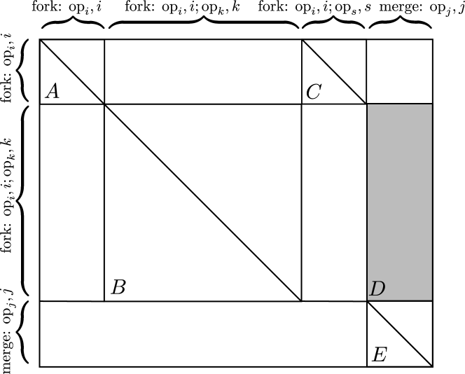Assigning all terms the described labels and subsequent numbering on each MPO bond yields $\widehat{W}^{s},\,s=1,\ldots,L$. Fig. 3 shows the result with labels sorted such that distinct subblocks can be recognized. From their labels we can infer the following properties:

$A$	One non-trivial operator ($\hat{c}^{\dagger}$ or $\hat{c}$) was applied to the left.
$B$	Continuation of terms with two non-trivial operators to the left (by means of identity operators).
$C$	The application of the second non-trivial operator (if $k=s$) takes the same input as $A$ but forks into labels with two operators, which will thus be part of the input to block $B$ and $D$ on the next site.
$D$	If $l=s$, the third non-trivial operator is multiplied by $V_{ijkl}$ and placed in block $D$. There exists a term for every possible combination of operators pairs on sites $i,k$ to the left and the operator on site $j$. Thus $D$ is dense.
$E$	Terms with three non-trivial operators on the left are extended by $\hat{F}$ operators to site $s+1$ to eventually connect to the last non-trivial operator on site $j$.

Both rows and columns contain labels with at most two positions, implying that the matrix size scales as $\mathcal{O}(L^{2})\times\mathcal{O}(L^{2})$. The cost of contracting the operator with the MPS on one site is proportional to the number of non-zero elements in the MPO matrix. As block $D$ has $\mathcal{O}(L^{2})$ rows and $\mathcal{O}(L)$ columns, the algorithm will scale as $\mathcal{O}(L^{4})$, because it performs $L$ iterations with a complexity of $\mathcal{O}(L^{3})$ in one sweep.

Note that the first and last operator (i.e. $s=i$ and $s=j$) of each term is missing in Fig. 3; their inclusion only adds a constant number of rows and columns to $\widehat{W}^{s}$ (one for each of $\hat{c}^{\dagger}_{\uparrow}$, $c^{\dagger}_{\downarrow}$, $\hat{c}_{\uparrow}$, $\hat{c}_{\downarrow}$ ). Terms omitted from the previous discussion may easily be accomodated in Fig. 3. The middle operator of two-electron terms with one matching pair of indices, for instance, will enter the square above block $D$.

Figure 3: MPO tensor $\widehat{W}^{s}_{b_{s-1}b_{s}}$ on some site $s$. $A$, $B$, $C$ and $E$ are diagonal blocks which extend incoming operator terms to the next site, while $D$ is dense and contains creation or annihilation operators multiplied by $V_{ijks}$. The first and last operator of each term, corresponding to $s=i$ and $s=j$, were omitted.

IV Fermionic anti-commutation

In the operator construction scheme that we described in the previous section we omitted the description of fermionic anticommutation.

$$\{\hat{c}^{\dagger}_{i\sigma},\hat{c}_{j\sigma^{\prime}}\} =\delta_{ij}\delta_{\sigma\sigma^{\prime}},$$

$$\{\hat{c}^{\dagger}_{i\sigma},\hat{c}^{\dagger}_{j\sigma^{\prime}}\}= \{\hat{c}_{i\sigma},\hat{c}_{j\sigma^{\prime}}\}=0.$$ (20)

We can can include it by performing a Jordan-Wigner transformation Jordan1928 on the elementary creation and annihilation operators. Introducing the auxiliary operator

$$\widehat{F}=\left(\begin{array}[]{c|cccc}&|\!\!\uparrow\!\downarrow\rangle&|\!\uparrow\,\rangle&|\!\downarrow\rangle&|\,0\,\rangle\\ \hline\cr|\!\!\uparrow\!\downarrow\rangle&1&0&0&0\\ |\!\uparrow\,\rangle&0&-1&0&0\\ |\!\downarrow\,\rangle&0&0&-1&0\\ |\,0\,\rangle&0&0&0&1\end{array}\right),$$ (21)

we transform each elementary creation or annihilation operator $\hat{\gamma}$ ($\hat{\gamma}=\hat{c}^{\dagger}_{\sigma},\,\hat{c}_{\sigma}$) as

$$\widehat{\gamma}_{i}\quad\mapsto\quad\Big{(}\prod_{s<i}\widehat{F}_{s}\Big{)}\widehat{\gamma}_{i}\quad=\quad\widehat{\gamma}^{\mathrm{JW}}_{i},$$ (22)

such that Eqs. (20) are fulfilled by the transformed operators. Since $\widehat{F}_{s}^{2}=\mathbb{I}$ and $[\widehat{F}_{s},\widehat{\gamma}_{i}]=0$ if $s\neq j$ , we can simplify

$$\widehat{\gamma}^{\mathrm{JW}}_{i}\widehat{\gamma}^{\mathrm{JW}}_{j}=\widehat{\mathbb{I}}_{1}\otimes\ldots\otimes\widehat{\gamma}_{i}\widehat{F}_{i}\otimes\widehat{F}_{i+1}\otimes\ldots\otimes\widehat{F}_{j-1}\otimes\widehat{\gamma}_{j},\otimes\ldots\otimes\widehat{\mathbb{I}}_{L}$$ (23)

and find that in terms with an even number of fermionic operators, the sign operators only have to be applied in sections with an odd number of fermions to the left.

The described transformation ensures that fermions on different sites anti-commute, but since the two kinds of electrons, $\uparrow$ and $\downarrow$, can coexist on the same site, we have to modify Eq. (22) in order to obtain the correct behavior: the operator $\hat{c}^{\dagger}_{\downarrow}$ has to be multiplied by $\widehat{F}$, yielding $\hat{c}^{\dagger}_{\downarrow}\widehat{F}$ prior to the transformation in Eq. (22) ($\hat{c}_{\downarrow}\mapsto\widehat{F}\hat{c}_{\downarrow}$ by hermitian conjugation). The additional sign operator keeps track of the phase factor incured by anti-commutation among electrons on the same site with opposite spin.

V MPS-MPO operations

Now that we have described the representation of many-electron states in the MPS format and the representation of arbitrary operators as MPOs, we would like to calculate ground-states of given Hamiltonians and subsequently compute expectation values on these states.

V.1 Expectation Values

Based on the definitions in Eqs. (4) and (11), we can immediately write down an expression for the transition operator matrix elements by introducing a second state

$$|\phi\rangle=\sum_{\bm{\sigma}}N^{\sigma_{1}}\,N^{\sigma_{2}}\,\cdots\,N^{\sigma_{L}}|\bm{\sigma}\rangle,$$ (24)

or for expectation values if $|\phi\rangle=|\psi\rangle$:

$$\langle\phi|\widehat{\mathcal{W}}|\psi\rangle=\sum_{\bm{\sigma\sigma^{\prime}}}\big{(} N^{\sigma_{1}}\cdots N^{\sigma_{L}}\big{)}^{*}\!\!\!\sum_{b_{1}\ldots b_{L-1}}\!\!\!\!W^{\sigma_{1}\sigma_{1}^{\prime}}_{1b_{1}}\cdots W^{\sigma_{L}\sigma_{L}^{\prime}}_{b_{L-1}1}$$

$$\cdot\,\big{(} M^{\sigma^{\prime}_{1}}\cdots M^{\sigma^{\prime}_{L}}\big{)},$$ (25)

denoting MPS tensors of $|\phi\rangle$ by $N$ and assuming $\langle\bm{\sigma}|\bm{\sigma^{\prime}}\rangle=\delta_{\bm{\sigma}\bm{\sigma^{\prime}}}$. This expression is exponentially expensive to evaluate, but suitable regrouping reduces the operation count to $\mathcal{O}(L^{4}m^{3})$:

$$\langle\phi|\widehat{\mathcal{W}}|\psi\rangle=\sum_{\sigma_{L}\sigma^{\prime}_{L},b_{L-1}}N^{\sigma_{L}\dagger}W^{\sigma_{L}\sigma_{L}^{\prime}}_{b_{L-1}1}\Bigg{(}\cdots\sum_{\sigma_{2}\sigma^{\prime}_{2},b_{1}}N^{\sigma_{2}\dagger}W^{\sigma_{2}\sigma_{2}^{\prime}}_{b_{1}b_{2}}$$

$$\qquad\qquad\cdot\Big{(}\sum_{\sigma_{1}\sigma^{\prime}_{1}}N^{\sigma_{1}\dagger}W^{\sigma_{1}\sigma_{1}^{\prime}}_{1b_{1}}M^{\sigma^{\prime}_{1}}\Big{)}M^{\sigma^{\prime}_{2}}\cdots\Bigg{)}M^{\sigma^{\prime}_{L}}.$$ (26)

The iterative character of the previous expression is already apparent from the fact that, proceeding from the innermost bracket outwards, at each step the tensor objects of the respective site are added to the contracted expression in the center. By introducing the initial value $\mathbb{L}^{0}_{b_{0}}=1$, $b_{0}=1$ we may thus translate Eq. (V.1) into an iterative equation:

$$\mathbb{L}^{l}_{b_{l}}=\sum_{\sigma_{l}\sigma^{\prime}_{l},b_{l-1}}N^{\sigma_{l}\dagger}W^{\sigma_{l}\sigma_{l}^{\prime}}_{b_{l-1}b_{l}}\mathbb{L}^{l-1}_{b_{l-1}}M^{\sigma^{\prime}_{l}}.$$ (27)

Since $N^{\sigma_{1}\dagger}$ and $M^{\sigma^{\prime}_{1}}$ each only have one column and one row, respectively (and $W^{\sigma_{l}\sigma_{l}^{\prime}}_{b_{l-1}b_{l}}$ beeing a scalar), the dimensions of matrix multiplications match at all steps. We refer to the objects $\mathbb{L}^{l}$ generated in this fashion as left boundaries, whose structure may be understood as a vector indexed by $b_{l}$. From Eqs. (27) and (3) we can further infer, that its elements are square matrices with indices $(a_{l},\,a_{l})$. The last boundary $\mathbb{L}^{L}$, is a scalar as well as the first, and, according to Eq. (V.1), equal to the desired expectation value.

Figure 4: Operations involved in enlarging the contracted left network $\mathbb{L}^{l-1}$ by one site to $\mathbb{L}^{l}$. Step 1: Contraction of $\mathbb{L}^{l-1}_{b_{l-1}}$ with the MPS tensor $M^{\sigma_{l}}$ (depicted as a set of four matrices, one for each value of $\sigma_{l}$) by matrix-matrix multiplication. Step 2: Summation over the local operator input $\sigma^{\prime}_{l}$ of $W^{\sigma_{l}\sigma^{\prime}_{l}}_{{b_{l-1}b_{l}}}$. Step 3: Summation over $b_{l-1}$. Step 4: Multiplication of $M^{\sigma_{l}\dagger}$ with the temporary $T_{b_{l}}$ and summation over $\sigma_{l}$ yields $\mathbb{L}^{l}_{b_{l}}$.

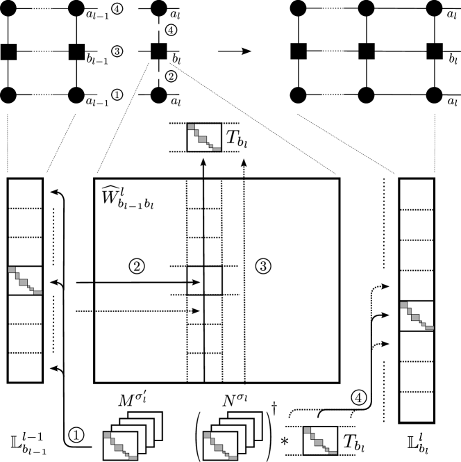
In Fig. 4, we illustrate the detailed operations contained in Eq. (27). The schematic representation in the upper part abstracts MPS tensors $M^{\sigma_{l}}_{a_{l-1}a_{l}}$ as circles and MPO tensors $W^{\sigma_{l}\sigma^{\prime}_{l}}_{b_{l-1}b_{l}}$ as squares. Both diagrams feature a leg for each tensor index sticking out and legs are connected to indicate a contraction over the two corresponding indices. In detail, the boundary propagation starts with the contraction of $\mathbb{L}^{l-1}_{b_{l-1}}$ and $M^{\sigma_{l}}$ by matrix-matrix multiplication (Fig. 4 step 1), after which the resulting products are multiplied by the MPO coefficient and have their quantum number mapped from $\sigma^{\prime}_{l}$ to $\sigma_{l}$ in step 2. As the final product with $N^{\sigma_{l}\dagger}$ does not involve $b_{l-1}$, the summation over $b_{l-1}$ into the temporary objects

$$T_{b_{l}}=\sum_{\sigma^{\prime}_{l},b_{l-1}}W^{\sigma_{l}\sigma_{l}^{\prime}}_{b_{l-1}b_{l}}\mathbb{L}^{l-1}_{b_{l-1}}M^{\sigma^{\prime}_{l}}.$$ (28)

is most efficiently performed at this stage (step 3) and finally followed by multiplication with the bra MPS tensor $N^{\sigma_{l}\dagger}$ (step 4), yielding $\mathbb{L}^{l}_{b_{l}}$.

At this point we remark, that we could have started to contract the tensors from the right hand side as well, which leads us to define right boundaries as

$$\mathbb{R}^{l-1}_{b_{l-1}}=\sum_{\sigma_{l}\sigma^{\prime}_{l},b_{l-1}}M^{\sigma^{\prime}_{l}}W^{\sigma_{l}\sigma_{l}^{\prime}}_{b_{l-1}b_{l}}\mathbb{R}^{l}_{b_{l}}N^{\sigma_{l}\dagger}.$$ (29)

From Eq. (V.1) we deduce that they can be assembled to yield the desired expectation value with a matching left boundary as

$$\langle\phi|\widehat{\mathcal{W}}|\psi\rangle=\sum_{b_{l}}\text{tr}\big{(}\mathbb{L}^{l}_{b_{l}}\mathbb{R}^{l}_{b_{l}}\big{)}.$$ (30)

While these variants may seem redundant at this point, they will later allow us to maximize the reuse of contracted objects during the sweeping procedure of the ground-state search.

V.2 Ground-state search

While in traditional DMRG, ground-states are determined by repeatedly diagonalizing a superblock Hamiltonian formed at shifting lattice bipartitions, in second generation DMRG discussed here, the energy is minimized through a variational search with the MPS tensor entries as parameters. According to standard MPS-DMRG theory Schollwock2011 ; Oestlund1995 , both approaches eventually result in the diagonalization of the same local Hamiltonian matrices, which is tackled by large sparse eigensolver techniques, such as Jacobi-Davidson. To clarify how both formulations are related, we first reconstruct the left and right block basis states as well as the superblock Hamiltonian from traditional DMRG in an MPO/MPS framework. Subsequently, we derive the same eigenvalue equation for the local site optimization from a variational viewpoint.

For a bipartition into $\mathcal{L}$ and $\mathcal{R}$ at site $l$, the left and right block basis states are given by

$$|a_{l-1}\rangle_{\mathcal{L}} =\sum_{\sigma_{1},\ldots,\sigma_{l-1}}\big{(}M^{\sigma_{1}}\cdots M^{\sigma_{l-1}}\big{)}_{1,a_{l-1}}|\sigma_{1},\ldots,\sigma_{l-1}\rangle$$ (31)

$$|a_{l}\rangle_{\mathcal{R}} =\sum_{\sigma_{l+1},\ldots,\sigma_{L}}\big{(}M^{\sigma_{l+1}}\cdots M^{\sigma_{L}}\big{)}_{a_{l},1}|\sigma_{l+1},\ldots,\sigma_{L}\rangle,$$ (32)

such that we can write the total state as

$$|\psi\rangle=\sum_{a_{l-1}a_{l},\sigma_{l}}M^{\sigma_{l}}_{a_{l-1},a_{l}}|a_{l-1}\rangle_{\mathcal{L}}|\sigma_{l}\rangle|a_{l}\rangle_{\mathcal{R}}.$$ (33)

The matrix elements of the superblock Hamiltonian $\langle a_{l-1}\sigma_{l}a_{l}|\widehat{\mathcal{H}}|a^{\prime}_{l-1}\sigma^{\prime}_{l}a^{\prime}_{l}\rangle$ can then be calculated by substituting $|a_{l-1}\rangle_{\mathcal{L}}$, $|a_{l}\rangle_{\mathcal{R}}$ and $\widehat{\mathcal{H}}$ with the corresponding MPO expressions, which leads to the eigenvalue problem

$$\varepsilon\,M^{\sigma_{l}}_{a_{l-1}a_{l}}=\sum_{a^{\prime}_{l-1}a^{\prime}_{l},\sigma_{l}}\!\!\!\!\!\langle a_{l-1}\sigma_{l}a_{l}|\widehat{\mathcal{H}}|a^{\prime}_{l-1}\sigma^{\prime}_{l}a^{\prime}_{l}\rangle\,\,M^{\sigma^{\prime}_{l}}_{a^{\prime}_{l-1}a^{\prime}_{l}}.$$ (34)

Alternatively, we can minimize the energy $\langle\psi|\widehat{\mathcal{H}}|\psi\rangle$ with respect to the entries of one MPS tensor $M^{\sigma_{l}}$ under the constraint that $\langle\psi|\psi\rangle=1$ and arrive at the same eigenvalue equation Oestlund1995 ; Schollwock2011 . Starting from Eq. (30), we first expose the coefficients $M^{\sigma_{l}}_{a_{l-1}a_{l}}$ in

$$\langle\psi|\widehat{\mathcal{H}}|\psi\rangle=\sum_{b_{l}}\,\,\, \text{tr}\big{(}\mathbb{L}^{l}_{b_{l}}\mathbb{R}^{l}_{b_{l}}\big{)}$$ (35)

$$=\sum_{b_{l-1}b_{l},\sigma_{l}\sigma^{\prime}_{l}}\!\!\!\!\!\! \text{tr}\big{(}M^{\sigma_{l}\dagger}W^{\sigma_{l}\sigma^{\prime}_{l}}_{b_{l-1}b_{l}}\mathbb{L}^{l-1}_{b_{l-1}}M^{\sigma^{\prime}_{l}}\mathbb{R}^{l}_{b_{l}},\big{)}$$ (36)

such that we can minimize the energy with respect to $M^{\sigma_{l}}_{a_{l-1}a_{l}}$ by introducing a Lagrangian multiplier $\lambda$: $\delta[\langle\psi|\widehat{\mathcal{H}}|\psi\rangle-\lambda(\langle\psi|\psi\rangle-1)]=0.$ Under the assumption that $\mathbb{L}^{l}_{b_{l}}$ and $\mathbb{R}^{l}_{b_{l}}$ were formed from left and right normalized MPS tensors respectively, the derivative of $\langle\psi|\psi\rangle$ with respect to $M^{\sigma_{l},\star}_{a_{l-1}a_{l}}$ is just $M^{\sigma_{l}}_{a_{l-1}a_{l}}$ and we arrive at the standard eigenvalue problem

$$\sum_{b_{l-1}b_{l},\sigma^{\prime}_{l}}\!\!\!\!\!\!W^{\sigma_{l}\sigma^{\prime}_{l}}_{b_{l-1}b_{l}}\mathbb{L}^{l-1}_{b_{l-1}}M^{\sigma^{\prime}_{l}}\mathbb{R}^{l}_{b_{l}}=\lambda M^{\sigma_{l}}.$$ (37)

The computationally relevant operation is the matrix-vector multiplication on the left hand side of the equation above as it is the key operation in sparse matrix eigensolvers. Looking at this operation in detail, we find that it is very similar to the boundary iteration in Eq. (27): steps 1–3 from Fig. 4 are identical, but instead of multiplying the temporaries $T_{b_{l}}$ by the MPS conjugate tensor, a scalar product with $\mathbb{R}^{l}_{b_{l}}$ is formed. With the implementation of Eqs. (27), (29), and (37) we have thus all operations at hand to compute ground-states of Hamiltonian MPOs. Moreover, in case of the quantum chemical Hamiltonian of Eq. (14), the compression technique described in this work ensures the optimal execution time scaling of $\mathcal{O}(m^{3}L^{3})+\mathcal{O}(m^{2}L^{4})$.

In addition to the eigenvalue problem in Eq. (37) for a single site, the procedure described in Ref. White2005 improves convergence by introducing a tiny ad-hoc noise term which helps to avoid local minima by re-shuffling the renormalized states.

V.3 Single-site and two-site DMRG

In the previous section, we described the optimization of a single site, which in practice has a high probability to become trapped in a local energy minimum. Although the convergence behaviour may be improved by introducing a tiny ad-hoc noise term White2005 , for chemical applications, the so-called two-site DMRG algorithm, in which two sites are optimized at the same time, achieves faster convergence and is much less likely to get stuck in local minima. In the MPS-MPO formalism, we can optimize two sites at once by introducing the two-site MPS tensor

$$P^{\sigma_{l}\sigma_{l+1}}_{a_{l-1}a_{l+1}}=\sum_{a_{l}}M^{\sigma_{l}}_{a_{l-1}a_{l}}M^{\sigma_{l+1}}_{a_{l}a_{l+1}}$$ (38)

and the two-site MPO tensor

$$\widehat{V}^{\sigma_{l}\sigma_{l+1}\sigma^{\prime}_{l}\sigma^{\prime}_{l+1}}_{b_{l-1}b_{l+1}}=\sum_{b_{l}}\widehat{W}^{\sigma_{l}\sigma_{l}^{\prime}}_{b_{l-1}b_{l}}\widehat{W}^{\sigma_{l+1}\sigma^{\prime}_{l+1}}_{b_{l}b_{l+1}}.$$ (39)

The latter case corresponds to a matrix-matrix multiplication of the operator valued $\widehat{W}$- matrices, whose entries are multiplied by forming the tensor product of the local site operators. If $\sigma_{l}\sigma_{l+1}=\sigma_{l}\otimes\sigma_{l+1}$ is treated as a single 16-dimensional local space $\tau_{l,l+1}$, we can extend Eq. (37) from the previous section to two-site DMRG by exchanging $M$ with $P$ and $W$ with $V$ and obtain

$$\sum_{b_{l-1}b_{l+1},\tau^{\prime}_{l,l+1}}\!\!\!\!\!\!V^{\tau_{l,l+1}\tau^{\prime}_{l,l+1}}_{b_{l-1}b_{l+1}}\mathbb{L}^{l-1}_{b_{l-1}}P^{\tau^{\prime}_{l,l+1}}\mathbb{R}^{l+1}_{b_{l+1}}=\lambda P^{\tau_{l,l+1}}.$$ (40)

The different steps in evaluating the above expression are essentially the same as for the single-site case, such that the same program routines can be used for both optimization schemes after the generation of the two-site tensors.

V.4 Excited states

The MPS-based state specific algorithm to economically calculate excited states McCulloch2007 repeatedly orthogonalizes the excited state against a supplied list of orthogonal states at every micro-iteration during the Jacobi-Davidson diagonalization step. Let $|\phi_{n}\rangle$ denote the $n$-th supplied orthogonal state and $|\psi\rangle$ the target wave function. We can then define the partial overlaps

$$C^{l}_{n}=\sum_{\sigma_{l}}M^{\sigma_{l}\dagger}\cdots\Big{(}\sum_{\sigma_{1}}M^{\sigma_{1}\dagger}N^{\sigma_{1}}_{n}\Big{)}\cdots N^{\sigma_{l}}_{n}$$ (41)

and

$$D^{l-1}_{n}=\sum_{\sigma_{l}}N^{\sigma_{l}}_{n}\cdots\Big{(}\sum_{\sigma_{L}}N^{\sigma_{L}}_{n}M^{\sigma_{L}\dagger}\Big{)}\cdots M^{\sigma_{l}\dagger},$$ (42)

where $|\phi_{n}\rangle$ and $|\psi\rangle$ are defined according to Eqs. (4) and (24), yielding $\langle\psi|\phi_{n}\rangle=\text{tr}(C^{l}_{n}D^{l}_{n})$ for the overlap.

At every site $l$, the orthogonal vectors $V_{n}$, which the Jacobi-Davidson eigensolver takes as input parameters, can now be calculated as

$$V_{n}=\sum_{\sigma_{l}}C^{l-1}_{n}N^{\sigma_{l}}_{n}D^{l}_{n}.$$ (43)

We note, that $V_{n}$ has the property $\text{tr}(M^{\sigma_{l}\dagger}V_{n})=\langle\psi|\phi_{n}\rangle$. After diagonalization, $C^{l}_{n}$ and $D^{l-1}_{n}$ are updated with the optimized $M^{\sigma_{l}}$ tensor during a left and right sweep respectively. Finally, the converged $|\psi\rangle$ will be orthogonal to all $|\phi_{n}\rangle$.

VI Calculations

Figure 5: Graphene fragments G2 (left) and G3 (right) with 24 and 54 $\pi$-orbitals, respectively.

The efficiency of an MPO DMRG implementation critically depends on the representation of the MPO. As we have shown, both a compact construction and the exploitation of sparsity are necessary to achieve optimal scaling.

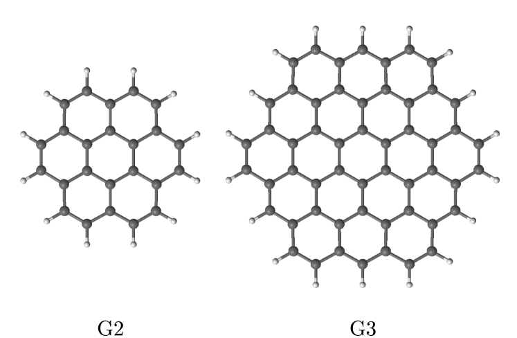
To demonstrate its capabilities, we calculated ground- and excited-state energies of the graphene fragments G2 and G3 shown in Fig. 5. The conjugation in both molecules provides for long-range correlation in two dimensions and they are therefore difficult to treat with DMRG, which performs best for one-dimensional and quasi one-dimensional systems. In other systems with less delocalization and mixed active spaces, containing both $\sigma$- and $\pi$-type molecular orbitals and possibly exhibiting spatial point group symmetry, often a significant fraction of the two-electron integrals have negligible magnitude, leading to smaller MPOs such that even larger active spaces become affordable.

Figure 6: Orbital ordering for the fragment G2. The mutal information between pairs of orbitals is drawn with bold black lines for magnitudes $>0.1$, dashed gray lines ($0.01-0.1$) and dotted green lines $(0.001-0.1)$.

We chose the $\pi$-orbitals for the active space, represented by a minimal STO-3G basis set Hehre1969 . While this choice of basis precludes obtaining realistic energies, it does not simplify the correlation problem within the active space, which we are interested to solve with DMRG. A set of different condensed polyaromatic systems has recently been calculated by Olivares-Amaya et al. in Ref. Chan2015 , employing the same basis set. In accordance with their work, we found that performing Pipek-Mezey localization Pipek1989 first within the active occupied orbitals, followed by a second Pipek-Mezey localization of the active virtual orbitals, provided the molecular orbital basis with the best convergence. The efficiency gain compared to Hartree-Fock orbitals more than compensated the loss of spatial point group symmetry.

Figure 7: Energy per carbon atom in G2 and G3, extrapolated towards truncation error $\varepsilon\rightarrow 0$. First panel: ground-state of G3 with m = 2000, 1500 and 1000. Second panel: lowest singlet excited-state of G2 with m = 1000, 950, 900, 850. Third panel: lowest triplet excited-state of G2 with m = 1000, 950, 900, 850. Fourth panel: ground-state of G2 with m = 350, 300, 250, 200 and a reference calculation with m = 3000.

In order to obtain accurate energies, we exploit non-abelian spin symmetry whose implementation with the quantum chemical DMRG Hamiltonian will be described in a later work SU2 . Furthermore, the type of orbitals and the orbital ordering have to be carefully chosen to improve performance. By computing the Fiedler vector Fiedler1973 ; Fiedler1975 ; Barcza2011 based on the mutual information Rissler2006 ; Legeza2006 , we determined an efficient orbital ordering. In Fig. 6, it is shown for the G2 fragment together with the mutual information drawn as lines with varying thickness according to entanglement strength. We observe that, based on this entanglement measure, the Fiedler ordering reliably grouped strongly entangled bonding and anti-bonding orbitals pairs next to each other and arranged orbitals according to their spatial position, such that the hexagonal fragment is traversed through the longest possible pathway across two adjacent corners. The application of the Fiedler ordering to G3 led a similar type of orbital arrangment.

With this configuration, we performed ground- and excited-state calculations with the implementation reported in this paper. The obtained energies per carbon atom are shown in Fig. 7. For the G2 ground-state calculation, $m$ was chosen such that we obtained truncation errors in the same range as the G3 ground-state calculation. This choice affords wavefunctions of similar quality in both cases and accordingly similar distances in the extrapolated energy, with the advantage, that for the smaller G2 fragment we can verify the extrapolation error with a precise reference calculation with $m=3000$. From the extrapolation, we estimate an error per carbon atom of $\pm 0.05\,\text{mH}$ for G2 and $\pm 0.1\,\text{mH}$ for G3, respectively.

VII Conclusions

In this work, we provided a prescription for the efficient construction of the quantum chemical Hamiltonian in Eq. (14) as an MPO. Our construction scheme ensures the same computational scaling as traditional DMRG, compared to which a similar performance can be achieved. The advantages of a full matrix product formulation of all wave functions and operators involved in the DMRG algorithm are the efficient calculation of low-lying excited states, straightforward implementation of new observables, and additional flexibility that allows us to accommodate different models and symmetries in a single source code. We investigated our MPO approach at the example of two graphene fragments of different sizes for which we calculated ground and excited state energies.

References

- (1) S. R. White, Phys. Rev. Lett. 69, 2863 (1992).
- (2) S. R. White, Phys. Rev. B 48, 10345 (1993).
- (3) K. H. Marti and M. Reiher, Z. Phys. Chem. 224, 583 (2010).
- (4) O. Legeza, R. M. Noack, J. Solyom, and L. Tincani, Lect. Notes Phys. 739, 653 (2008).
- (5) G. K.-L. Chan and S. Sharma, Ann. Rev. Phys. Chem. 62, 465 (2011).
- (6) S. Wouters and D. Van Neck, Eur. Phys. J. D 68, 272 (2014).
- (7) Y. Kurashige, Mol. Phys. 112, 1485 (2014).
- (8) T. Yanai, Y. Kurashige, W. Mizukami, J. Chalupsky, T. N. Lan, and M. Saitow, Int. J. Quant. Chem. 115, 283 (2015).
- (9) S. Szalay, M. Pfeffer, V. Murg, G. Barcza, F. Verstraete, R. Schneider, and O. Legeza, Int. J. Quant. Chem. 115, 1342 (2015).
- (10) K. H. Marti and M. Reiher, Phys. Chem. Chem. Phys. 13, 6750 (2011).
- (11) S. Östlund and S. Rommer, Phys. Rev. Lett. 75, 3537 (1995).
- (12) G. Vidal, J. Latorre, E. Rico, and A. Kitaev, Phys. Rev. Lett. 90, 227902 (2003).
- (13) T. Barthel, M.-C. Chung, and U. Schollwöck, Phys. Rev. A 74, 022329 (2006).
- (14) N. Schuch, M. M. Wolf, F. Verstraete, and J. I. Cirac, Phys. Rev. Lett. 100, 030504 (2008).
- (15) J. D. Bekenstein, Phys. Rev. D 7, 2333 (1973).
- (16) M. Srednicki, Phys. Rev. Lett. 71, 666 (1993).
- (17) F. Verstraete, D. Porras, and J. I. Cirac, Phys. Rev. Lett. 93, 227205 (2004).
- (18) I. P. McCulloch, J. Stat. Mech. Theor. Exp. , P10014 (2007).
- (19) G. M. Crosswhite, A. C. Doherty, and G. Vidal, Phys. Rev. B 78, 035116 (2008).
- (20) F. Verstraete, J. J. García-Ripoll, and J. I. Cirac, Phys. Rev. Lett. 93, 207204 (2004).
- (21) S. Wouters, W. Poelmans, P. W. Ayers, and D. V. Neck, Comput. Phys. Commun 185, 1501 (2014).
- (22) J. Rissler, R. M. Noack, and S. R. White, Chem. Phys. 323, 519 (2006).
- (23) K. Boguslawski, P. Tecmer, G. Barcza, O. Legeza, and M. Reiher, J. Chem. Theory Comput. 9, 2959 (2013).
- (24) M. Dolfi, B. Bauer, S. Keller, A. Kosenkov, T. Ewart, A. Kantian, T. Giamarchi, and M. Troyer, Comput. Phys. Commun. 185, 3430 (2014).
- (25) K. H. Marti, I. Malkin Ondik, G. Moritz, and M. Reiher, J. Chem. Phys. 128, 014104 (2008).
- (26) Y. Kurashige and T. Yanai, J. Chem. Phys. 135, 094104 (2011).
- (27) S. Sharma and G. K.-L. Chan, J. Chem. Phys. 136, 124121 (2012).
- (28) U. Schollwöck, Ann. Phys. 326, 96 (2011).
- (29) G. Moritz and M. Reiher, J. Chem. Phys. 126, 244109 (2007).
- (30) G. K. L. Chan, J. Chem. Phys. 120, 3172 (2004).
- (31) O. Legeza, J. Röder, and B. A. Hess, Phys. Rev. B 67, 124114 (2003).
- (32) O. Legeza and J. Solyom, Phys. Rev. B 70, 205118 (2004).
- (33) K. Boguslawski, K. H. Marti, and M. Reiher, J. Chem. Phys. 134, 224101 (2011).
- (34) B. Bauer, P. Corboz, R. Orús, and M. Troyer, Phys. Rev. B 83, 125106 (2011).
- (35) S. White and R. Martin, J. Chem. Phys. 110, 4127 (1999).
- (36) G. M. Crosswhite and D. Bacon, Phys. Rev. A 78, 012356 (2008).
- (37) P. Jordan and E. Wigner, Z. Phys. 47, 631 (1928).
- (38) S. R. White, Phys. Rev. B 72, 180403 (2005).
- (39) W. J. Hehre, R. F. Stewart, and J. A. Pople, J. Chem. Phys. 51, 2657 (1969).
- (40) R. Olivares-Amaya, W. Hu, N. Nakatani, S. Sharma, J. Yang, and G. K.-L. Chan, J. Chem. Phys. 142, (2015).
- (41) J. Pipek and P. G. Mezey, J. Chem. Phys. 90, 4916 (1989).
- (42) S. Keller and M. Reiher, Spin-adapted MPO-based DMRG for quantum chemistry, in preparation.
- (43) M. Fiedler, Czech. Math. J. 23, 298 (1973).
- (44) M. Fiedler, Czech. Math. J. 25, 607 (1975).
- (45) G. Barcza, O. Legeza, K. H. Marti, and M. Reiher, Phys. Rev. A 83, 012508 (2011).
- (46) O. Legeza, F. Gebhard, and J. Rissler, Phys. Rev. B 74, 195112 (2006).