Concentration phenomenon in some non-local equation
Abstract.
We are interested in the long time behaviour of the positive solutions of the Cauchy problem involving the following integro-differential equation
together with the initial condition in . Such a problem is used in population dynamics models to capture the evolution of a clonal population structured with respect to a phenotypic trait. In this context, the function represents the density of individuals characterized by the trait, the domain of trait values is a bounded subset of , the kernels and respectively account for the competition between individuals and the mutations occurring in every generation, and the function represents a growth rate. When the competition is independent of the trait, we construct a positive stationary solution which belongs to the space of Radon measures on . Morever, when this “stationary” measure is regular and bounded, we prove its uniqueness and show that, for any non negative initial datum in , the solution of the Cauchy problem converges to this limit measure in . We also construct an example for which the measure is singular and non-unique, and investigate numerically the long time behaviour of the solution in such a situation. These numerical simulations seem to reveal some dependence of the limit measure with respect to the initial datum.
Dedicated to the Professor Stephen Cantrell, with all our admiration.
1. Introduction and Main results
In this paper, we are interested in the evolution of a clonal population structured with respect to a phenotypic trait and essentially subjected to three processes: mutation, growth, and competition. As an example, one can think of a virus population structured by its virulence, as this trait can be easily quantified from experimental data. For such type of population, a common model used (see [8, 7, 19, 21, 9, 10, 28, 12, 11, 29, 30]) is the following:
| (1.1) | |||
| (1.2) |
the function being the density of individuals of the considered population characterized by the trait , the set is a bounded domain of , the function and respectively are a competition kernel and a growth rate, and is a linear diffusion operator modelling the mutation process. In the literature, depending on the context, several kinds of mutation operator have been considered, see [8, 7, 21, 9, 1, 12, 18, 24, 29, 27, 25] among others. In the present work, we focus our analysis on populations for which is an integral operator of the form
| (1.3) |
with a positive kernel satisfying some integrability conditions.
Lately, this type of equation have attracted a lot of attention and much effort has been made in the analysis of solutions of (1.1). In particular, let us mention [9, 10, 18, 11] for the construction of a global solution in for any non negative initial data in and quite fairly general assumptions on , , and . We also point to [29, 11, 30] for an analysis of the existence of bounded continuous stationary solutions and their local stability for unidimensional domains . However, the analysis of stationary solutions of (1.1) in higher dimension remains to be done, while the long time behaviour of positive solutions of problem (1.1)-(1.2) is still not fully understood.
When mutations are neglected (that is, ), equation (1.1) is reduced to
| (1.4) |
and, for a generic positive initial datum , the solution to (1.4)-(1.2) is known to converge weakly to a positive Radon measure [20, 18, 23]. This measure is, in some sense, a stationary solution of (1.4) representing an evolutionarily stable strategy for the system. For example, when the kernel is positive and does not depend on the trait (i.e., ), is a measure whose support lies in the set . In such a situation, one may check that a sum of Dirac masses , with for all , is a stationary solution. When this measure is unique, then the positive solution of (1.4)– (1.2) converges weakly to , see [23] for a detailed proof.
Since the mutation process can be seen as a diffusion operator on the trait space, it is expected that the long time behaviour of a positive solution to (1.1)–(1.2) is simple and that such concentration phenomena does not occur. Indeed, this conjecture can be verified when the mutation operator is a classical elliptic operator [24, 14]. When it is an integral operator as in the present situation, the existence of bounded equilibria when is unidimensional seems to give credit to this conjecture. However, we prove that it is false in higher dimension. To this end, we exhibit a class of situations in which a positive singular measure , solution of (1.1) can be constructed, and investigate numerically the long time behaviour of positive solutions of the corresponding Cauchy problem.
1.1. Main results
We first state precisely the assumptions on the domain , the kernels and and the function under which the results are obtained. We suppose that the domain is an open bounded connected set of with Lipschitz boundary, that the function is such that
| (1.5) |
and that is a non-negative symmetric Carathéodory kernel function, that is, , and
| (1.6) |
Finally, we assume that the kernel is independent of the trait (i.e., ) and that it satisfies the following condition: there exist positive constants such that
| (1.7) |
where denotes the characteristic function of the set .
Let us now consider a stationary solution of (1.1), that is, satisfying
| (1.8) |
Under the above assumptions, we prove that there exists a positive Radon measure solution of (1.8) in a weak sense.
Theorem 1.1.
Assume and satisfy (1.5)–(1.7). Then there exists a positive Radon measure such that for all in ,
| (1.9) |
Let be the principal eigenvalue of the operator defined by
Then, we have the following characterisation for the measure .
-
•
If is associated with an eigenfunction which belongs to , then is a regular (uniformly continuous) measure, that is, with in and is the unique strong solution of (1.8). Moreover, is in when the principal eigenfunction belongs to .
-
•
Otherwise, is a singular measure.
As a consequence from the above dichotomy result, the existence of singular measure for (1.9) is strongly related to the non-existence of a eigenfunction associated with . This non-existence result has recently been established for the non-local operator , as shown in [13, 32, 15].
Next, we analyse the global stability of and the long time behaviour of the positive solution of (1.1)–(1.2). When the measure is regular, we have the following result.
Theorem 1.2.
Note that the above global stability implies the uniqueness of the regular stationary positive Radon measure solution of (1.8). When no regular positive Radon measure exists, the convergence of a positive solution of (1.1) is very delicate to analyse. To shed light on the possible dynamics in such a situation, we explore numerically the behaviour of solutions of (1.1)–(1.2).
1.2. Numerical simulations
In order to illustrate and get some insight on the long time behaviour of solutions to (1.1)–(1.2), we numerically solve the problem for different choices of growth function and initial datum in two dimensions. Limiting ourselves to preliminary computations, we choose the domain as the open ball of radius centered at the origin, that is, , and the competition and mutation kernels uniformly constant, such that and with a positive constant. The system to be numerically solved thus reduces to:
| (1.10) | |||
| (1.11) |
1.2.1. A simple growth rate
First, we look at a situation in which the growth rate achieves its maximum at a single point, a case for which we can show the uniqueness of the stationary solution. More precisely, we have the following result.
Proposition 1.3.
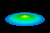
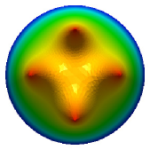
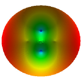
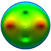
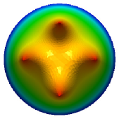
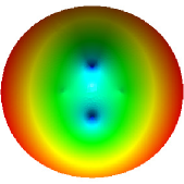
For any positive value , there exists a unique positive measure which is a stationary solution of (1.10). Moreover, there exists a critical value such that the measure is singular for , whereas it is regular for . In addition, for any non negative initial datum in , the solution of (1.10) converges weakly to .
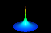
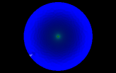
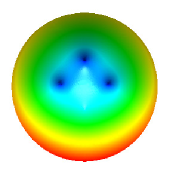
This proposition is a direct consequence of Theorem 1.1 and of the uniform estimates obtained in Section 3. To illustrate its conclusions, we take , where denotes the Euclidean norm in (, ), and solve numerically the problem. The obtained results, presented in Figure 1, provide a clear picture of the dynamics of the solution.

1.2.2. A complex growth rate
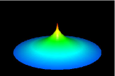
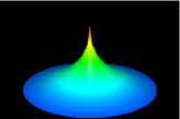
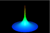
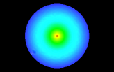
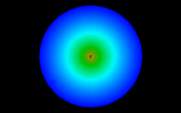
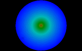
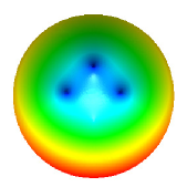
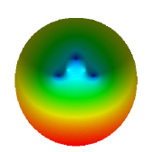
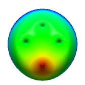
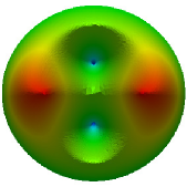
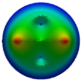
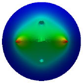
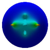
Next, we explore a situation where the growth rate achieves its maximum at multiple points. In such a setting, we expect the stationary measure to be non-unique. In order to verify this conjecture numerically, we consider a function of the form:
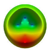
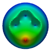
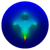
which achieves its maximum at four distinct points. With this choice, for sufficiently small, we can show that there is at least four different positive Radon measures that are solution of the stationary problem (1.9). The impact of the non-uniqueness of the stationary measure simulations can be seen in the simulations prensented in Figures 2 and 3. Indeed, in a regime of mutation rate where several singular stationary measures can be constructed, we observe that the outcome of the simulation may drastically differ depending on the initial datum (see Figures 3 and 4). In contrast, in a regime where the mutation rate is such that the stationary measure is regular, the stationary solution is a global attractor (see Figure 2).
1.3. Outline
The paper is organised as follows. We start by recalling in Section 2 important facts about the spectral properties of the class of non-local operators considered in the problem. We then derive some uniform estimates by means of nonlinear relative entropy formulas in Section 3 and give a proof of Theorems 1.1 and 1.2 in Section 4. Finally, the numerical method used for the simulations is briefly described in an appendix section.


2. Spectral properties of non-local operators
In this section, we recall some known results on the spectral problem
| (2.1) |
where is the integral operator defined by (1.3) with a kernel satisfying the assumption (1.6). When the function is not constant, neither the operator nor its inverse are compact, and the Krein-Rutman theory fails in providing existence of the principal eigenvalue of . However, a variational formula, introduced in [4] to characterise the first eigenvalue of elliptic operators, can be transposed to the operator . Namely, the following quantity
| (2.2) |
is well defined and called the generalised principal eigenvalue of . It is known [13, 32, 17, 2, 31] that is not always an eigenvalue of in a reasonable Banach space, which means there is not always a positive continuous eigenfunction associated with it. Nevertheless, as shown in [15], there always exists an associated positive Radon measure.
Theorem 2.1 ([15]).
Let the domain be bounded, the operator be defined by (1.3) with a kernel satisfying (1.6), be a continuous function over , and define
Then, there exists a positive Radon measure , such that, for any in , we have
In addition, we have the following dichotomy:
-
•
either there exists in , , such that ,
-
•
or there exists in , , and a positive singular measure with respect to the Lebesgue measure, whose support lies in the set , such that
The measure can be characterised more precisely and there exists a simple criterion guaranteeing its regularity.
Proposition 2.2 ([13, 17, 2, 16]).
Under the assumptions of the preceding theorem, with , , if and only if .
We conclude by recalling a characterisation of in the spirit of what is known for elliptic operators [5, 3, 6].
As in the case of elliptic operators, the two quantities and are equal in our setting.
3. A priori estimates
In this section, for a non-negative initial data in , we establish some uniform in time a priori estimates on the solution of (1.1)–(1.2). To do so, we start by proving a non-linear relative entropy identity satisfied by any solution of (1.1).
Proposition 3.1 (general identity).
Let be a bounded domain and assume that and satisfies (1.5)–(1.7). Let be a smooth (at least ) function. Let be a positive stationary solution of (1.1). Let be a solution of (1.1), then we have
| (3.1) |
where , , are defined by
Proof:From (1.1), since the kernel satisfies condition (1.7), by defining we have for all
Using that is a positive stationary solution of (1.1), for almost every , we have
and we can rewrite the above equation as follows
Multiplying the above identity by and integrating over , we find that
By rearranging the terms, we get
and, due to the symmetry of , we straightforwardly see that
Hence, by combining the above equalities, we reach
Remark 3.2.
Remark 3.3.
Equipped with this general relative entropy identity, we may derive some useful differential inequalities.
Proposition 3.4.
Let be a bounded domain and assume that and satisfies (1.5)–(1.7). Let and be the smooth convex function . Let be two positive solutions of (1.1) as in Proposition 3.1. Then the functional satisfies:
| (3.2) |
Moreover, we have
| (3.3) |
Remark 3.5.
We observe that in the case of , and we get a Lyapunov functional involving the norm of instead of a weighted norm of . Indeed, we have
Proof of Proposition 3.4:Observe that, for , we have, by Proposition 3.1,
Therefore, by definition of we get from the above equality
| (3.4) |
Now by taking in (3.4), we obtain
A quick computation shows that and therefore
| (3.5) |
Since for all , for all times, we have
| (3.6) | |||
| (3.7) |
By combining (3.6) and (3.7), we end up with
Equality (3.3) then follows straightforwardly from direct computations, by using symmetry and an obvious change of variables.
From these differential inequalities, we obtain uniform in time a priori bounds of the norm of a solution of (1.1) – (1.2). Namely, we show
Lemma 3.6.
Proof:
First, let us observe that large (respectively small) constants are super-solutions (respectively sub-solutions) of (1.1). Indeed, for , we have
Similarly, for , we get
Therefore, from Proposition 3.1 and Remark 3.3, by choosing a large, respectively a small constant, and considering the convex function , we get
Now, since satisfies (1.7), we have for all and from the above differential inequalities we get
From the logistic character of these two differential inequalities and since , we deduce that for all
Remark 3.7.
Observe that the above proof holds as well for bounded above and below by positive constants. As a consequence, such a uniform estimate can be also obtained in a more general situation where the kernel is not necessarily independent of the trait .
4. Proofs
We are now in a position to prove Theorems 1.1 and 1.2. Let us start with the construction of a stationary measure.
4.1. Construction of a Stationary state
Consider the stationary problem (1.8), then in order to construct stationary state in the space of Radon measures, we have to find solution of the following weak formulation
| (4.1) |
Owing to Theorem 2.1, let us consider a positive measure associated to , which we normalise in order to have .
Claim 4.1.
There exists a unique such that is a positive stationary solution of (4.1).
Proof:Let be defined by . For any , satisfies
Thus, is a stationary solution of (4.1).
To conclude, it remains to show that . This is the case, since we have by Theorem 2.4, and by taking as test function, we can easily check that
Remark 4.2.
From the above computation, we clearly see that the uniqueness of the stationary state follows from the uniqueness of the measure associated with .
4.2. Long time behaviour
Let us now prove Theorem 1.2. We assume that the positive measure constructed above is regular and bounded, i.e. with . Since is associated with the principal eigenvalue , then with and defined in the proof of Claim 4.1. From the regularity of , we can see that is a strong solution of (1.8). Now, knowing that a positive continuous stationary solution of (1.8) exists, we can derive further a priori estimates on the solution of (1.1)–(1.2).
Lemma 4.3.
Proof:The uniform lower bound is rather easy to obtain and follows directly from the Hölder’s inequality and the estimates in Lemma 3.6. Indeed, since is bounded we have
where denotes the Lebesgue measure of the set .
On the other hand, we get an uniform upper bound as a straightforward application of Proposition 3.4. Namely, since is a positive stationary solution of (1.1), by Proposition 3.4, the functional is a decreasing function of and therefore, for all ,
Hence, for all ,
In order to prove that converges to a stationary solution, we introduce the following decomposition of . Since for all , and belong to , they belong to and we can write as follows:
with such that for all .
Claim 4.4.
and as .
Proof:For convenience, we introduce the following notation to denote the standard scalar product of two function of .
We start by deriving some useful bounds on and . From the decomposition, we have
Therefore, since is positive and bounded in , we have from Lemma 3.6
and
| (4.2) |
From Lemma 4.3, we obviously derive an upper bound for . Indeed, by construction
| (4.3) |
Substituting to its decomposition in the equation (1.1), we get
| (4.4) |
Multiplying the above equation by and integrating it over , we get after obvious computations
where we used the definition of and .
Since , we get
By following the computation developed for the proof of Proposition 3.1 with , we see that
| (4.5) |
with .
By construction, for all . So either for all times or there exists such that . In the latter case, we have for almost every . Let with satisfying the ODE
| (4.6) | |||
| (4.7) |
By construction, as and we can check that is a solution of (1.1) for all . Thus, since by uniqueness of the solution of the Cauchy problem (1.1), we have for all and therefore for all , and .
In the other situation, for all and we claim the following.
Claim 4.5.
as .
Assume the Claim holds then we can conclude the proof by arguing as follows. From the decomposition , we can express the function by . Using Proposition 3.4, we deduce that
| (4.8) |
Now by using as , we deduce that
with .
Therefore, by a elementary analysis of the ODE, we deduce that as .
Proof of Claim 4.5:Since for all , from (4.5) and by following the proof of Proposition 3.4 we see that
| (4.9) |
Thus is a non increasing smooth function. Thanks the monotonicity of , to prove the Claim, it is sufficient to exhibit a sequence such that and .
To exhibit such sequence, it is sufficient to prove that . By contradiction, let us assume that . Then, by (4.2) and (4.3), there exist positive constants such that for all
As a consequence, there exists such that
| (4.10) |
Take now a sequence such that , and consider the sequence of functions . Then is then bounded from above and below and therefore, by (4.10) and (4.9), we get
| (4.11) |
On the other hand, since is bounded in , there exists such that, up to extraction of a subsequence, in . Let us evaluate . Since and are positive and bounded from above and below, the function , is well defined and for some positive constant . Moreover, we have
| (4.12) |
Since and , by Fatou’s Lemma and the weak convergence of , we get
Therefore,
which enforces that for some constant . Recall now that for all , , so
implying that . Now since, and , from (4.11) and (4.12), we get
which leads to the following contradiction
Hence, , and since , this implies that
Acknowledgements
The research leading to these results has received funding from the french ANR program under the “ANR JCJC” project MODEVOL: ANR-13-JS01-0009 held by Gael Raoul and the ANR "DEFI" project NONLOCAL: ANR-14-CE25-0013 held by Francois Hamel. J. Coville also wants to thank Professor Raoul for interesting discussions on this topic.
Appendix A Numerical Aspects
To investigate numerically the behaviour of the solution of (1.10), we are led to understand how to solve numerically evolution problems of the form :
| (A.1) | |||
| (A.2) |
To solve numerically (A.1)–(A.2), our approach is to rewrite the above problem in a variational form and use a finite element method. Multiplying (A.1) by and integrating over , we get
| (A.3) |
To approximate the time derivation, we use standard Euler approximation scheme. For the space discretisation of , we use the standard Lagrange finite elements. Let us look at the non-local term. If we set,
where is the element of a finite element basis. Then, for , we have
which can be rewritten as follows
| (A.4) |
If we interpolate the map on the fem basis of , we have
| (A.5) |
Plugging the interpolation (A.5) in the relation (A.4), we get
which rewrites
| (A.6) |
Now set and to be the following square matrices
Then (A.6) can be expressed as follows:
| (A.7) |
The finite element matrix representing the integral term is then given by the multiplication of three matrices . Thus
| (A.8) |
With this finite element approximation of the integral terms, we implement a standard Euler semi-implicit scheme using FreeFem++ [22] to compute numerically the solution of (1.1)–(1.2). To guarantee the convergence of the scheme used, the mesh used is an adapted mesh composed of approximately 17000 triangles.
References
- [1] G. Barles and B. Perthame, Dirac concentrations in Lotka-Volterra parabolic PDEs, Indiana Univ. Math. J. 57 (2008), no. 7, 3275–3302.
- [2] H. Berestycki, J. Coville, and H. Vo, Properties of the principal eigenvalue of some nonlocal operators, preprint, 2014.
- [3] H. Berestycki, F. Hamel, and L. Rossi, Liouville-type results for semilinear elliptic equations in unbounded domains, Ann. Mat. Pura Appl. (4) 186 (2007), no. 3, 469–507.
- [4] H. Berestycki, L. Nirenberg, and S. R. S. Varadhan, The principal eigenvalue and maximum principle for second-order elliptic operators in general domains, Comm. Pure Appl. Math. 47 (1994), no. 1, 47–92.
- [5] H. Berestycki and L. Rossi, On the principal eigenvalue of elliptic operators in and applications, J. Eur. Math. Soc. (JEMS) 8 (2006), no. 2, 195–215.
- [6] by same author, Reaction-diffusion equations for population dynamics with forced speed. I. The case of the whole space, Discrete Contin. Dyn. Syst. 21 (2008), no. 1, 41–67.
- [7] R. Bürger, The mathematical theory of selection, recombination, and mutation, Wiley series in mathematical and computational biology, John Wiley, 2000.
- [8] R. Bürger and J. Hofbauer, Mutation load and mutation-selection-balance in quantitative genetic traits, J. Math. Biol. 32 (1994), no. 3, 193–218.
- [9] A. Calsina and S. Cuadrado, Stationary solutions of a selection mutation model: the pure mutation case, Math. Models Methods Appl. Sci. 15 (2005), no. 7, 1091–1117.
- [10] by same author, Asymptotic stability of equilibria of selection-mutation equations, J. Math. Biol. 54 (2007), no. 4, 489–511.
- [11] A. Calsina, S. Cuadrado, L. Desvillettes, and G. Raoul, Asymptotics of steady states of a selection-mutation equation for small mutation rate, Proc. Roy. Soc. Edinburgh Sect. A 143 (2013), no. 6, 1123–1146.
- [12] N. Champagnat, R. Ferrière, and S. Méléard, Individual-based probabilistic models of adaptive evolution and various scaling approximations, Seminar on Stochastic Analysis, Random Fields and Applications V (R. C. Dalang, F. Russo, and M. Dozzi, eds.), Progress in Probability, vol. 59, Birkhaüser Basel, 2008, pp. 75–113.
- [13] J. Coville, On a simple criterion for the existence of a principal eigenfunction of some nonlocal operators, J. Differential Equations 249 (2010), no. 11, 2921 – 2953.
- [14] by same author, Convergence to the equilibria on some mutation selection model, preprint, 2012.
- [15] by same author, Singular measure as principal eigenfunction of some nonlocal operators, Appl. Math. Lett. 26 (2013), no. 8, 831–835.
- [16] by same author, Nonlocal refuge model with a partial control, Discrete Contin. Dynam. Systems 35 (2015), no. 4, 1421–1446.
- [17] J. Coville, J. Dávila, and S. Martínez, Pulsating fronts for nonlocal dispersion and KPP nonlinearity, Ann. Inst. H. Poincaré Anal. Non Linéaire 30 (2013), no. 2, 179–223.
- [18] L. Desvillettes, P. E. Jabin, S. Mischler, and G. Raoul, On selection dynamics for continuous structured populations, Comm. Math. Sci. 6 (2008), no. 3, 729–747.
- [19] O. Diekmann, A beginner’s guide to adaptive dynamics, Banach Center Publ. 63 (2003), 47–86.
- [20] O. Diekmann, P. E. Jabin, S. Mischler, and B. Perthame, The dynamics of adaptation: an illuminating example and a Hamilton-Jacobi approach, Theoret. Population Biol. 67 (2005), no. 4, 257–271.
- [21] N. Fournier and S. Méléard, A microscopic probabilistic description of a locally regulated population and macroscopic approximations, Ann. Appl. Probab. 14 (2004), no. 4, 1880–1919.
- [22] F. Hecht, New development in FreeFem++, J. Numer. Math. 20 (2012), no. 3-4, 251–265.
- [23] P. E. Jabin and G. Raoul, On selection dynamics for competitive interactions, J. Math. Biol. 63 (2011), no. 3, 493–517.
- [24] A. Lorz, S. Mirrahimi, and B. Perthame, Dirac mass dynamics in multidimensional nonlocal parabolic equations, Comm. Partial Differential Equations 36 (2011), no. 6, 1071–1098.
- [25] S. Méléard and S. Mirrahimi, Singular limits for reaction-diffusion equations with fractional Laplacian and local or nonlocal nonlinearity, Comm. Partial Differential Equations 40 (2015), no. 5, 957–993.
- [26] P. Michel, S. Mischler, and B. Perthame, General relative entropy inequality: an illustration on growth models, J. Math. Pures Appl. (9) 84 (2005), no. 9, 1235–1260.
- [27] S. Mirrahimi and G. Raoul, Dynamics of sexual populations structured by a space variable and a phenotypical trait, Theoret. Population Biol. 84 (2013), 87–103.
- [28] B. Perthame, From differential equations to structured population dynamics, Transport Equations in Biology, Frontiers in Mathematics, vol. 12, Birkhaüser Basel, 2007, pp. 1–26.
- [29] G. Raoul, Long time evolution of populations under selection and vanishing mutations, Acta Appl. Math. 114 (2011), no. 1, 1–14.
- [30] by same author, Local stability of evolutionary attractors for continuous structured populations, Monatsh. Math. 165 (2012), no. 1, 117–144.
- [31] W. Shen and X. Xie, On principal spectrum points/principal eigenvalues of nonlocal dispersal operators and applications, Discrete Contin. Dyn. Syst. 35 (2015), no. 4, 1665–1696.
- [32] W. Shen and A. Zhang, Spreading speeds for monostable equations with nonlocal dispersal in space periodic habitats, J. Differential Equations 249 (2010), no. 4, 747–795.